RM3-TH/01-7

ROME1-1326/01

Next-to-Leading Order QCD Corrections
to Spectator Effects
in Lifetimes of Beauty Hadrons

M. Ciuchini^a, E. Franco^b, V. Lubicz^a and F. Mescia^b

^a Dip. di Fisica, Univ. di Roma Tre and INFN, Sezione di Roma III,
Via della Vasca Navale 84, I-00146 Rome, Italy
^b Dip. di Fisica, Univ. di Roma “La Sapienza” and INFN, Sezione di Roma,
P.le A. Moro 2, I-00185 Rome, Italy

1 Introduction

The calculation of inclusive decay rates of hadrons containing a $b$ quark can be performed by computing the amplitude through an Operator Product Expansion (OPE) in powers of $\Lambda_{QCD}/m_{b}$ [1, 2]. This allows a quantitative evaluation of the hadronic decay rates under the assumption that properly smeared partonic amplitudes can replace the hadronic ones. This assumption is usually referred to as the “quark-hadron duality”, which in the case of total rates is required to hold in its local formulation [3]-[5], namely the smearing is provided by the sum over exclusive states.

Within this theoretical framework, and up to terms of ${\cal O}(1/m_{b}^{2})$, only the $b$ quark enters the short-distance weak decay, while the light quarks in the hadron interact through soft gluons only. In particular, the leading term in the expansion reproduces the results of the old spectator model, thus providing a theoretical basis to this model. Quantitatively, however, the contributions to the lifetimes ratios of the first two terms in the OPE are too small. Neglecting terms of ${\cal O}(1/m_{b}^{3})$, one finds

$$\frac{\tau(B^{+})}{\tau(B_{d})}=1.00\,,\qquad\frac{\tau(B_{s})}{\tau(B_{d})}=1.00\,,\qquad\frac{\tau(\Lambda_{b})}{\tau(B_{d})}=0.98(1)\,,$$ (1)

to be compared with the experimental measurements [6]

$$\frac{\tau(B^{+})}{\tau(B_{d})}=1.07\pm 0.02\,,\qquad\frac{\tau(B_{s})}{\tau(B_{d})}=0.95\pm 0.04\,,\qquad\frac{\tau(\Lambda_{b})}{\tau(B_{d})}=0.80\pm 0.06\,.$$ (2)

Given the discrepancies, it is important to understand whether we are facing a signal of quark-hadron duality violation or, instead, the inclusion of higher-order terms in $\Lambda_{QCD}/m_{b}$ and $\alpha_{s}$ is sufficient to reproduce the data.

Spectator contributions, which appear at ${\cal O}(1/m_{b}^{3})$ in the OPE, can explain the lifetime differences, as they distinguish the light-quark content of the hadrons. As observed by Neubert and Sachrajda [7], these effects, although suppressed by an additional power of $1/m_{b}$, are enhanced with respect to leading contributions by a phase-space factor $16\pi^{2}$, being $2\to 2$ processes instead of $1\to 3$ decays. The calculation of spectator effects at the leading order (LO) in QCD has been done few years ago [7, 8] and a phenomenological analysis has been presented in ref. [7]. By using the recent lattice calculations of the relevant four-fermion operator matrix elements [9]-[12], we obtain the LO predictions

$$\left.\frac{\tau(B^{+})}{\tau(B_{d})}\,\right|_{\rm LO}\!\!\!\!\!=1.01\pm 0.03\,,\qquad\left.\frac{\tau(B_{s})}{\tau(B_{d})}\,\right|_{\rm LO}\!\!\!\!\!=1.00\pm 0.01\,,\qquad\left.\frac{\tau(\Lambda_{b})}{\tau(B_{d})}\,\right|_{\rm LO}\!\!\!\!\!=0.93\pm 0.04\,,$$ (3)

in agreement with previous estimates. The errors include the uncertainty due to the variation of the renormalization scale $\mu$ between $m_{b}/2$ and $2m_{b}$. For the ratio $\tau(\Lambda_{b})/\tau(B_{d})$, the inclusion of spectator contributions reduces the discrepancy between theoretical and experimental determinations while, for $B$ mesons, at the LO, no significant improvement is seen.

In this paper we compute the next-to-leading order (NLO) QCD corrections to the coefficient functions of the valence operators contributing to spectator effects. Our calculation has been performed in the limit of vanishing charm quark mass, which means that corrections of the order of $\alpha_{s}m_{c}^{2}/m_{b}^{2}$ have been neglected. The main motivations to improve the leading-order results are

• reducing the large renormalization-scale dependence which appears at the LO [7];

• properly taking into account in the matching the renormalization-scheme dependence of the Wilson coefficients and of the operator matrix elements;

• increasing the accuracy of the theoretical predictions by evaluating ${\cal O}(\alpha_{s})$ corrections which are potentially large.

Using the results of the NLO calculation, and the available lattice determinations of the hadronic matrix elements [9]-[12], we have also performed in this paper a phenomenological analysis of the lifetime ratios. We find that the inclusion of NLO QCD corrections to spectator effects improves the agreement between theoretical predictions of lifetime ratios and their measured values. We obtain the estimates

$$\left.\frac{\tau(B^{+})}{\tau(B_{d})}\,\right|_{\rm NLO}\!\!\!\!\!=1.07\pm 0.03\,,\qquad\left.\frac{\tau(B_{s})}{\tau(B_{d})}\,\right|_{\rm NLO}\!\!\!\!\!=1.00\pm 0.01\,,\qquad\left.\frac{\tau(\Lambda_{b})}{\tau(B_{d})}\,\right|_{\rm NLO}\!\!\!\!\!=0.89\pm 0.05\,,$$ (4)

to be compared with the experimental determinations given in eq. (2). The lifetime ratio of charged to neutral $B$-mesons turns out to be in very good agreement with the experimental data. In the case of the $B_{s}$ meson and the $\Lambda_{b}$ baryon the agreement is at the 1$\sigma$ level. We should also mention, however, that, in the baryon case, the lattice evaluation of the relevant matrix elements is still preliminary [10].

An important check of our perturbative calculation is provided by the cancellation of the infrared (IR) divergences in the expressions of the coefficient functions, in spite these divergences appear in the individual amplitudes. Their presence provides an example of violation of the Bloch-Nordsieck theorem in non-abelian gauge theories. We have also checked that our results are explicitly gauge invariant and have the correct ultraviolet (UV) renormalization-scale dependence as predicted by the known anomalous dimensions of the relevant operators.

The OPE of the lifetime ratios is expressed in terms of local operators defined in the Heavy Quark Effective Theory (HQET). The non-perturbative lattice determination of the hadronic matrix elements has been performed, in some cases, in terms of operators defined in QCD. In order to combine these determinations with the results obtained for the Wilson coefficients, consistently at the NLO, a matching between QCD and the HQET operators must be performed. In this paper, we have computed this matching, at ${\cal O}(\alpha_{s})$, in the case of the flavour non-singlet $\Delta B=0$ four fermion operators, for which the lattice results are available so far.

The NLO predictions of the lifetime ratios may still be improved in several ways. These improvements concern both the perturbative and the non-perturbative part of the calculation, and are:

• the charm quark mass corrections, of the order $\alpha_{s}m_{c}^{2}/m_{b}^{2}$, to the Wilson coefficients are still unknown. Such a calculation is in progress;

• the NLO coefficient functions of the current-current operators containing the charm quark field and the penguin operator (see eqs. (14) and (15)) have not been computed yet. The non-perturbative determination of the corresponding matrix elements is also missing. These contributions do not affect the theoretical determination of $\tau(B^{+})/\tau(B_{d})$ and are an $SU(3)$-breaking effect for $\tau(B_{s})/\tau(B_{d})$. In the case of $\tau(\Lambda_{b})/\tau(B_{d})$, however, their effects may not be negligible;

• the NLO anomalous dimension of the relevant operators in the HQET is still unknown. For this reason, present lattice calculations of the $\Lambda_{b}$ matrix elements [10, 11] only achieve a LO accuracy. For $B$ mesons, a complete NLO determination has been performed on the lattice by using operators defined in QCD [12];

• in the lattice determination of the hadronic matrix elements, penguin contractions (i.e. eye diagrams), which contribute in the case of flavour non-singlet operators, have not been computed. These contributions cancel in the evaluation of the ratio $\tau(B^{+})/\tau(B_{d})$ but affect $\tau(\Lambda_{b})/\tau(B_{d})$ and $\tau(B_{s})/\tau(B_{d})$, the latter through $SU(3)$-breaking effects.

The above discussion shows that, while the theoretical determination of $\tau(B^{+})/\tau(B_{d})$ can be considered as rather accurate, in the case of $\tau(B_{s})/\tau(B_{d})$ and $\tau(\Lambda_{b})/\tau(B_{d})$ some ingredients are still missing, and their determination may further improve the agreement with the experimental data.

The plan of this paper is the following. In sect. 2 we give the relevant formulae for the decay rate of $b$-hadrons. The details of the calculation are given in sect. 3, while our results are summarized in sect. 4. In sect. 5 we present the results of the matching between QCD and HQET operators for the flavour non-singlet sector. Finally, the phenomenological analysis is presented in sect. 6.

2 The inclusive decay width of beauty hadrons

Using the optical theorem, the inclusive decay width of a hadron $H_{b}$ containing a $b$ quark can be written as the imaginary part of the forward matrix element of the transition operator ${\cal T}$

$$\Gamma(H_{b}\to X)=\frac{1}{M_{H_{b}}}{\mathrm{I}m}\langle H_{b}|{\cal T}|H_{b}\rangle=\frac{1}{2M_{H_{b}}}\langle H_{b}|\widehat{\Gamma}|H_{b}\rangle\,,$$ (5)

where ${\cal T}$ is given by

$${\cal T}=i\int d^{4}x\;T\left({\cal H}_{eff}^{\Delta B=1}(x){\cal H}_{eff}^{\Delta B=1}(0)\right)\,.$$ (6)

The operator ${\cal H}_{eff}^{\Delta B=1}$ is the effective weak hamiltonian which describes $\Delta B=1$ transitions. It has the form

$${\cal H}_{eff}^{\Delta B=1}=\frac{G_{F}}{\sqrt{2}}\Bigg{\{}\Bigg{[}\Bigg{(}V^{\ast}_{cb}V_{us}\left(C_{1}Q_{1}+C_{2}Q_{2}\right)+V^{\ast}_{cb}V_{cs}\left(C_{1}Q^{c}_{1}+C_{2}Q^{c}_{2}\right)+\left(c\leftrightarrow u\right)\Bigg{)}-$$

$$\qquad V^{\ast}_{tb}V_{ts}\left(\sum_{i=3}^{6}C_{i}Q_{i}+C_{8G}Q_{8G}\right)+\left[s\to d\right]\Bigg{]}+\mathop{\displaystyle\sum}_{l=e,\mu,\tau}\left(V^{\ast}_{cb}Q_{l}^{c}+V^{\ast}_{ub}Q_{l}^{u}\right)\Bigg{\}}+h.c.\,,$$ (7)

where $C_{i}$ are the Wilson coefficients, known at the NLO in perturbation theory [13]-[15], and the operators $Q_{i}$ are defined as

$$\begin{array}[]{ll}Q_{1}=(\bar{b}_{i}c_{j})_{V-A}(\bar{u}_{j}s_{i})_{V-A}\,,&Q_{2}=(\bar{b}_{i}c_{i})_{V-A}(\bar{u}_{j}s_{j})_{V-A}\,,\\ Q^{c}_{1}=(\bar{b}_{i}c_{j})_{V-A}(\bar{c}_{j}s_{i})_{V-A}\,,&Q^{c}_{2}=(\bar{b}_{i}c_{i})_{V-A}(\bar{c}_{j}s_{j})_{V-A}\,,\\ Q_{3}=(\bar{b}_{i}s_{i})_{V-A}\mathop{\displaystyle\sum}\limits_{q}(\bar{q}_{j}q_{j})_{V-A}\,,&Q_{4}=(\bar{b}_{i}s_{j})_{V-A}\mathop{\displaystyle\sum}\limits_{q}(\bar{q}_{j}q_{i})_{V-A}\,,\\ Q_{5}=(\bar{b}_{i}s_{i})_{V-A}\mathop{\displaystyle\sum}\limits_{q}(\bar{q}_{j}q_{j})_{V+A}\,,&Q_{6}=(\bar{b}_{i}s_{j})_{V-A}\mathop{\displaystyle\sum}\limits_{q}(\bar{q}_{j}q_{i})_{V+A}\,,\\ Q_{8G}={\displaystyle{g_{s}\over 8\pi^{2}}}m_{b}\bar{b}_{i}\sigma^{\mu\nu}\left(1-\gamma^{5}\right)t^{a}_{ij}s_{j}G^{a}_{\mu\nu}&Q_{l}^{q}=(\bar{b}_{i}q_{i})_{V-A}(\bar{\nu}_{l}l)_{V-A}\,.\end{array}$$ (8)

Here and in the following we use the notation $(\bar{q}q)_{V\pm A}=\bar{q}\gamma_{\mu}(1\pm\gamma_{5})q$. A sum over colour indices is always understood. We also neglect Cabibbo-suppressed terms in eq. (2), so that the effective $\Delta B=1$ hamiltonian reduces to

$${\cal H}_{eff}^{\Delta B=1} = \frac{G_{F}}{\sqrt{2}}V^{\ast}_{cb}\Bigg{\{}C_{1}\left[(\bar{b}_{i}c_{j})_{V-A}(\bar{u}_{j}d_{i})_{V-A}+(\bar{b}_{i}c_{j})_{V-A}(\bar{c}_{j}s_{i})_{V-A}\right]+$$

$$\qquad\quad~{}\,C_{2}\left[(\bar{b}_{i}c_{i})_{V-A}(\bar{u}_{j}d_{j})_{V-A}+(\bar{b}_{i}c_{i})_{V-A}(\bar{c}_{j}s_{j})_{V-A}\right]+$$

$$\qquad\quad~{}\sum_{i=3}^{6}C_{i}Q_{i}+C_{8G}Q_{8G}+\mathop{\displaystyle\sum}_{l=e,\mu,\tau}Q_{l}^{c}\,\Bigg{\}}+h.c.\,.$$

In the double insertion of the $\Delta B=1$ effective hamiltonian, this corresponds to neglecting terms suppressed by $m_{c}^{2}/m_{b}^{2}\sin^{2}\theta_{c}$ with respect to the dominant ones.

Because of the large mass of the $b$ quark, it is possible to construct an OPE for the transition operator ${\cal T}$ of eq. (5), which results in a sum of local operators of increasing dimension [1, 2]. We include in this expansion terms up to ${\cal O}(1/m_{b}^{2})$ plus those $1/m_{b}^{3}$ corrections that come from spectator effects and are enhanced by the phase space. The resulting expression for the local $\Delta B=0$ operator $\widehat{\Gamma}$, of eq. (5), is

$$\widehat{\Gamma}=\frac{G_{F}^{2}|V_{cb}|^{2}m_{b}^{5}}{192\pi^{3}}\left[c^{(3)}\bar{b}b+c^{(5)}\frac{g_{s}}{m_{b}^{2}}\bar{b}\sigma_{\mu\nu}G^{\mu\nu}b+\frac{96\pi^{2}}{m_{b}^{3}}\mathop{\displaystyle\sum}_{k}c^{(6)}_{k}O_{k}^{(6)}\right]\,,$$ (10)

where the $O_{k}^{(6)}$ are a set of four-fermion dimension-six operators to be specified below. These operators represent the contribution of hard spectator effects. At the lowest order in QCD, the diagrams entering the calculation of $\widehat{\Gamma}$ are shown in fig. 1.

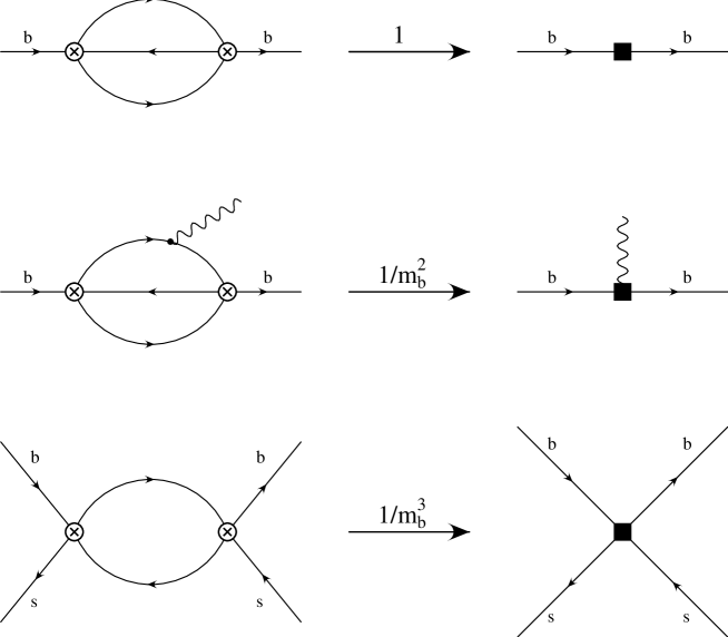
Figure 1: Examples of LO contributions to the transition operator ${\cal T}$ (left) and to the corresponding local operator $\widehat{\Gamma}$ (right). The crossed circles represent the insertions of the $\Delta B=1$ effective hamiltonian. The black squares represent the insertion of a $\Delta B=0$ operator.

We notice that, in general, the OPE of $\widehat{\Gamma}$ cannot be expressed in terms of local operators defined in QCD. The reason is that, in full QCD, renormalized operators mix with operators of lower dimension with coefficients proportional to powers of the $b$-quark mass. In this way, the dimensional ordering of the OPE is lost. In order to implement the expansion, the matrix elements of the local operators should be cut-off at a scale smaller than the $b$-quark mass. This is naturally realized by defining the operators in the HQET.

From eqs. (5) and (10), one can derive an expression for the ratio of inclusive widths

$${\displaystyle{\Gamma(H_{b})\over\Gamma(H_{b}^{\prime})}}={\displaystyle{M_{H_{b}^{\prime}}\langle\bar{b}b\rangle_{H_{b}}\over M_{H_{b}}\langle\bar{b}b\rangle_{H_{b}^{\prime}}}}\left({\displaystyle{1+{\displaystyle{g_{s}\over m_{b}^{2}}}{\displaystyle{c^{(5)}\over c^{(3)}}}{\displaystyle{\langle\bar{b}\sigma_{\mu\nu}G^{\mu\nu}b\rangle_{H_{b}}\over\langle\bar{b}b\rangle_{H_{b}}}}+{\displaystyle{96\pi^{2}\over m_{b}^{3}}}\mathop{\displaystyle\sum}\limits_{k}{\displaystyle{c^{(6)}_{k}\langle O_{k}\rangle_{H_{b}}\over c^{(3)}\langle\bar{b}b\rangle_{H_{b}}}}\over 1+{\displaystyle{g_{s}\over m_{b}^{2}}}{\displaystyle{c^{(5)}\over c^{(3)}}}{\displaystyle{\langle\bar{b}\sigma_{\mu\nu}G^{\mu\nu}b\rangle_{H_{b}^{\prime}}\over\langle\bar{b}b\rangle_{H_{b}^{\prime}}}}+{\displaystyle{96\pi^{2}\over m_{b}^{3}}}\mathop{\displaystyle\sum}\limits_{k}{\displaystyle{c^{(6)}_{k}\langle O_{k}\rangle_{H_{b}^{\prime}}\over c^{(3)}\langle\bar{b}b\rangle_{H_{b}^{\prime}}}}}}\right)\,,$$ (11)

where $\langle\cdots\rangle_{H}$ denotes the forward matrix element between two hadronic states $H$ defined with the covariant normalization. The matrix elements of dimension-three and dimension-five operators, appearing in eq. (11), can be expanded using the HQET

$$\langle\bar{b}b\rangle_{H_{b}} = 2M_{H_{b}}\left(1-\frac{\mu_{\pi}^{2}(H_{b})-\mu_{G}^{2}(H_{b})}{2m_{b}^{2}}+{\cal O}(1/m_{b}^{3})\right)\,,$$

$$g_{s}\langle\bar{b}\sigma_{\mu\nu}G^{\mu\nu}b\rangle_{H_{b}} = 2M_{H_{b}}\left(2\mu^{2}_{G}(H_{b})+{\cal O}(1/m_{b})\right)\,.$$ (12)

By substituting these expansions in eq. (11), we finally obtain

$${\displaystyle{\Gamma(H_{b})\over\Gamma(H_{b}^{\prime})}} = 1-\frac{\mu_{\pi}^{2}(H_{b})-\mu_{\pi}^{2}(H_{b}^{\prime})}{2m_{b}^{2}}+\left(\frac{1}{2}+\frac{2c^{(5)}}{c^{(3)}}\right)\frac{\mu_{G}^{2}(H_{b})-\mu_{G}^{2}(H_{b}^{\prime})}{m_{b}^{2}}+$$ (13)

$$\quad{\displaystyle{96\pi^{2}\over m_{b}^{3}\,c^{(3)}}}\mathop{\displaystyle\sum}\limits_{k}c^{(6)}_{k}\left(\frac{\langle O^{(6)}_{k}\rangle_{H_{b}}}{2M_{H_{b}}}-\frac{\langle O_{k}^{(6)}\rangle_{H_{b}^{\prime}}}{2M_{H_{b}^{\prime}}}\right)\,,$$

which is the expression used in the evaluation of the lifetime ratios of beauty hadrons.

The Wilson coefficients $c^{(3)}$ and $c^{(5)}$ in eq. (13) have been computed at the LO in ref. [16], while the NLO corrections to $c^{(3)}$ have been evaluated in [17]-[22]. The NLO corrections to $c^{(5)}$ are still missing. Their numerical contribution to the lifetime ratios, however, is expected to be negligible.

The dimension-six operators in eq. (13), which express the hard spectator contributions, are the current-current operators

$$\begin{array}[]{ll}O^{q}_{1}=(\bar{b}b)_{V-A}(\bar{q}q)_{V-A}\,,&O^{q}_{2}=(\bar{b}b)_{V+A}(\bar{q}q)_{V-A}\,,\\ O^{q}_{3}=(\bar{b}t^{a}b)_{V-A}(\bar{q}t^{a}q)_{V-A}\,,&O^{q}_{4}=(\bar{b}t^{a}b)_{V+A}(\bar{q}t^{a}q)_{V-A}\,,\end{array}$$ (14)

with $q=u,d,s,c$, and the penguin operator

$$O_{P}=(\bar{b}_{i}t^{a}_{ij}b_{j})_{V}\mathop{\displaystyle\sum}\limits_{q=u,d,s,c}(\bar{q}_{k}t^{a}_{kl}q_{l})_{V}\,.$$ (15)

In these definitions, the symbols $b$ and $\bar{b}$ denote the heavy quark fields in the HQET. Note that the operator basis in eq. (14) differs from the one used in ref. [7] by a Fierz rearrangement. Our choice of the basis is more convenient for NLO calculations because it does not require the introduction of Fierz-evanescent operators in the intermediate steps of the calculation.

The coefficient functions of the current operators $O^{q}_{k}$, have been computed at the LO in ref. [7] for $q=u,d,s$, and in ref. [23] for the charm quark operator. The coefficient function of the penguin operator $O_{P}$ vanishes at the LO.

In this paper we have computed the NLO QCD corrections to the coefficient functions of the operators $O^{q}_{k}$ with $q=u,d,s$. The operators containing the charm quark fields contribute, as valence operators, only to the inclusive decay rate of $B_{c}$ mesons, and their contribution to non-charmed hadron decay rates is expected to be negligible. The calculation of the NLO corrections to these coefficient functions, as well as the NLO calculation of the coefficient function of the penguin operator, has not been performed yet.

3 Details of the perturbative calculation

In this section we summarize the general formulae used in the matching procedure, and present the details of our calculation. The matching condition between the transition operator in eq. (6) and the width operator in eq. (10) can be written in the form

$$Im\,\langle{\cal T}\rangle\sim\vec{c}^{\,T}(\mu)\langle\vec{O}(\mu)\rangle\,,$$ (16)

where $\langle\cdots\rangle$ indicates the matrix element computed between a common pair of partonic external states. We are using the vector notation for both coefficients and operators. The condition (16) determines the Wilson coefficients $\vec{c}$ at the matching scale $\mu$.

We expand at ${\cal O}(\alpha_{s})$ the matrix elements in eq. (16) and express the result in terms of tree-level matrix elements $\langle\vec{O}\rangle_{0}$

$$Im\,\langle{\cal T}\rangle = \left(\vec{T}_{0}+\frac{\alpha_{s}}{4\pi}\vec{T}_{1}\right)^{T}\langle\vec{O}\rangle_{0}^{QCD}\,,$$

$$\langle\vec{O}(\mu)\rangle = \left(1+\frac{\alpha_{s}}{4\pi}\hat{s}\right)\langle\vec{O}\rangle_{0}^{HQET}\,,$$ (17)

We also consider the perturbative expansion for the Wilson coefficients,

$$\vec{c}=\vec{c}_{0}+\frac{\alpha_{s}}{4\pi}\vec{c}_{1}\,.$$ (18)

Up to $1/m_{b}$ corrections, the tree-level matrix elements of the operators in QCD are equal to their HQET counterparts so that, by using eqs. (16)–(18), we readily find the matching conditions at the scale $\mu$

$$\vec{c}_{0}=\vec{T}_{0}\,,\qquad\vec{c}_{1}=\vec{T}_{1}-\hat{s}^{T}\,\vec{T}_{0}\,.$$ (19)

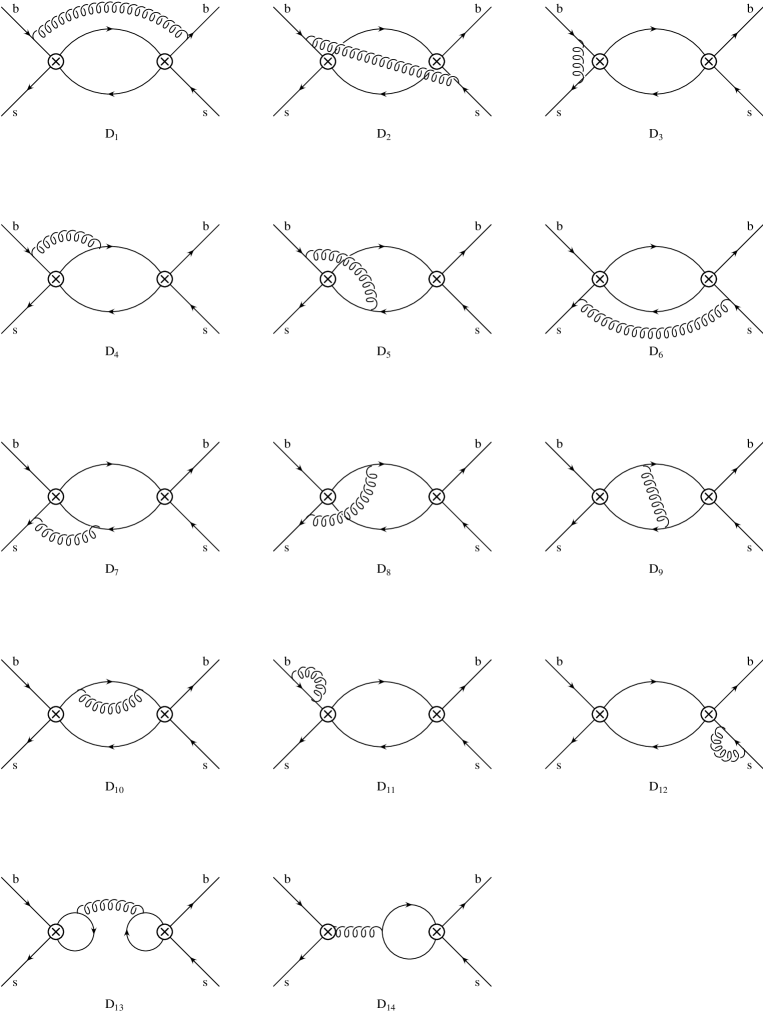
Figure 2: Feynman diagrams which contribute at NLO to the matrix element of the transition operator ${\cal T}$ in the case $q=s$. In the other cases, $q=u,\,d$, diagrams $D_{13}$ and $D_{14}$ do not contribute.

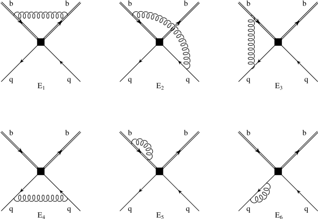
Figure 3: Feynman diagrams which contribute at NLO to the matrix element of the $\Delta B=0$ operators entering the width operator $\widehat{\Gamma}$.

In order to obtain $\vec{T}_{1}$ and $\hat{s}$, we have first computed in QCD the imaginary part of the diagrams shown in fig. 2 (full theory) and then, in the HQET, the diagrams shown in fig. 3 (effective theory). The external quark states have been taken on-shell and all quark masses, except $m_{b}$, have been neglected. More specifically, we have chosen the heavy quark momenta $p_{b}^{2}=m_{b}^{2}$ in QCD and $k_{b}=0$ in the HQET, and $p_{q}=0$ for all light quarks. In this way, we automatically retain the leading term in the $1/m_{b}$ expansion. We have performed the calculation in a generic covariant gauge, in order to check the gauge independence of the final results. Two-loop integrals have been reduced to a set of known (massless $p$- and massive tadpole) integrals using the recurrence relation technique [24]-[26]. Equations of motion have been used to reduce the number of independent operators. The $\Delta B=0$ operators in the HQET have been renormalized in the $\mbox{NDR-}\overline{\rm{MS}}$ scheme defined in details in ref. [27].

Some diagrams, both in the full and in the effective theory, are plagued by IR divergences. These are diagrams where a soft gluon is exchanged between the external legs ($D_{1}$, $D_{2}$, $D_{3}$, $D_{6}$ in fig. 2 and all the diagrams in fig. 3) . The divergences do not cancel in the final partonic amplitudes, and provide an example of violation of the Bloch-Nordsieck theorem in non-abelian gauge theories [28]–[30]. In agreement with this theorem, we explicitly verified that the abelian combination of the diagrams does not contain IR divergences. They only appear when the colour structure is taken into account. According to the KLN theorem [31, 32], IR singularities cancel when the contribution of soft gluons in the initial state is included in the amplitudes. Even if the amplitudes in the full and effective theories are IR divergent, we expect the IR poles to cancel in the matching, since the Wilson coefficients must be insensitive to soft physics. We have explicitly checked that, in the computation of the coefficient functions $c^{(6)}$, this cancellation takes place.

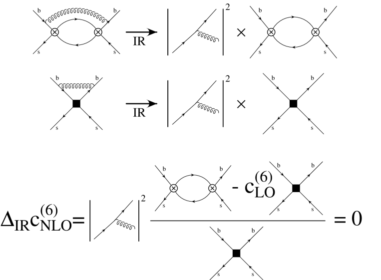
Figure 4: Example of the mechanism that guarantees the vanishing of IR contributions to the coefficient functions. Only the contributions from diagrams $D_{1}$ and $E_{1}$ are shown. In the presence of dimensionally-regularized IR divergences, LO matching up to and including terms of ${\cal O}(\varepsilon)$ is required.

We use $D$-dimensional regularization with anticommuting $\gamma_{5}$ (NDR) to regularize both UV and IR divergences. The presence of dimensionally-regularized IR divergences introduces subtleties in the matching procedure. Usually, the matching can be performed by only considering the four dimensional operator basis, since renormalized evanescent operators do not give contributions to the physical amplitudes. In the present case, however, IR poles in $\varepsilon=(4-D)/2$ promote the ${\cal O}(\varepsilon)$ contribution from evanescent operators to finite terms in the $D\to 4$ limit. This contribution has to be taken into account and the matching procedure must be consistently performed at ${\cal O}(\varepsilon)$. To illustrate this point in further details, we provide the example in fig. 4. Let us consider the IR-divergent parts of the diagrams $D_{1}$ and $E_{1}$. These divergences are not expected to give contribution to the Wilson coefficients, since the coefficients should only account for the UV behaviour of the effective theory. This condition is in fact guaranteed by the factorization of IR divergences and by the LO matching condition. Indeed, the numerator entering the definition of $\Delta_{IR}c^{(6)}_{\rm NLO}$ in fig. 4, which represents the IR contribution to the coefficient function $c^{(6)}$ at the NLO, vanishes just because of the LO matching condition. This happens provided that IR divergences are regularized in the same way in the full and in the effective theory, independently of the specific choice of the IR regulator. In this way, soft physics does not enter the coefficient functions. If, however, IR divergences are dimensionally regularized, the condition $\Delta_{IR}c^{(6)}_{\rm NLO}=0$ only holds when the LO matching condition is performed up to and including terms of ${\cal O}(\varepsilon)$. In particular, $D$-dimensional matching requires enlarging the operator basis to include (renormalized) evanescent operators, which must be inserted in the one-loop diagrams of the effective theory. Because of the IR divergences, the matrix elements of the renormalized evanescent operators do not vanish in the $D\to 4$ limit.

A similar discussion concerning the matching procedure in the presence of IR divergences can be found in ref. [33]. We mention that the relevant evanescent operators, which enter the matching in our calculation, are

$$\begin{array}[]{ll}E_{1}^{q}=\bar{b}\gamma_{\mu}\gamma_{\alpha}\gamma_{\nu\,L}b\;\bar{q}\gamma^{\nu}\gamma^{\alpha}\gamma^{\mu}_{L}q-4\,O^{q}_{1}\,,&E_{3}^{q}=\bar{b}\gamma_{\mu}\gamma_{\alpha}\gamma_{\nu\,L}t^{a}b\;\bar{q}\gamma^{\nu}\gamma^{\alpha}\gamma^{\mu}_{L}t^{a}q-4\,O^{q}_{3}\,,\\ E_{2}^{q}=\bar{b}\gamma_{\mu}\gamma_{\alpha}\gamma_{\nu\,R}b\;\bar{q}\gamma^{\nu}\gamma^{\alpha}\gamma^{\mu}_{L}q-16\,O^{q}_{2}\,,&E_{4}^{q}=\bar{b}\gamma_{\mu}\gamma_{\alpha}\gamma_{\nu\,R}t^{a}b\;\bar{q}\gamma^{\nu}\gamma^{\alpha}\gamma^{\mu}_{L}t^{a}q-16\,O^{q}_{4}\,.\end{array}$$ (20)

The procedure for taking into account their contribution is further discussed in the Appendix. We have also checked, on a proper subset of gauge-invariant diagrams, that a calculation using the gluon mass as IR regulator gives the same result as the one obtained with dimensional regularization by performing the matching at ${\cal O}(\varepsilon)$, and including the insertion of the evanescent operators.

We conclude this section by mentioning that our calculation of the Wilson coefficients has passed the following checks:

• gauge invariance: we verified that the coefficients are explicitly gauge-invariant. The same is true for the full and the effective amplitudes separately;

• renormalization-scale dependence: the coefficient functions have the correct renormalization-group behaviour as predicted by the LO anomalous dimension matrix of the $\Delta B=0$ operators;

• IR divergences: the coefficient functions are infrared finite. The cancellation of IR divergences also takes place for the abelian combination of diagrams in both the full and the effective amplitudes.

4 Spectator contributions at the NLO

In this section we present the results for the coefficient functions of the dimension-six operators $O_{k}^{q}$ of eq. (14) for $q=u,d,s$. We collect the known LO expressions and then present our new results for the NLO contributions.

The width operator $\widehat{\Gamma}$ in eq. (5) depends quadratically on the coefficient functions $C_{i}$ of the $\Delta B=1$ effective hamiltonian. Therefore, we find convenient to write the coefficient functions of the dimension-six operators as

$$c^{q}_{k}(\mu)=\sum_{i,j=1,2}C_{i}(\mu_{1})\,C_{j}(\mu_{1})\,F^{q}_{k,ij}(\mu_{1},\mu)\,,$$ (21)

where $\mu_{1}$ is the renormalization scale of the $\Delta B=1$ effective hamiltonian and $\mu$ is the renormalization scale of the $\Delta B=0$ operators entering the expansion of $\widehat{\Gamma}$ . The coefficients $F^{q}_{k,ij}$ depend on the renormalization scheme and scale of both the $\Delta B=0$ and $\Delta B=1$ operators. The dependence on $\mu_{1}$ and on the renormalization scheme of the $\Delta B=1$ operators actually cancels, order by order in perturbation theory, against the corresponding dependence of the $\Delta B=1$ Wilson coefficients $C_{i}$. Therefore, the coefficient functions $c^{q}_{k}$ only depend on the renormalization scheme of the $\Delta B=0$ operators. A given scheme of the $\Delta B=1$ operators, however, must be chosen in order to present results for $F^{q}_{k,ij}$. In the following we always consider $\Delta B=1$ operators renormalized in the $\mbox{NDR-}\overline{\rm{MS}}$ scheme, defined in details in ref. [34]. The corresponding Wilson coefficients can be found in refs. [13]-[15].

Since we use dimensional regularization to regularize both UV and IR divergences, the scales $\mu$ and $\mu_{1}$ in eq. (21) play the rôle of both renormalization scale and IR regulator. Dimensionally-regularized IR divergences produce additional $\log\mu$ and $\log\mu_{1}$, beside those governed by the renormalization-group equations. In the matching procedure, the same IR regulators in the full and effective theories must be used, therefore we have to identify $\mu$ and $\mu_{1}$. This choice gets rid of the spurious $\log(\mu/\mu_{1})$ so that the NLO coefficient functions have the correct UV behaviour predicted by the LO anomalous dimensions of the $\Delta B=0$ operators.

For the coefficients $F^{q}_{k,ij}$ we write the expansion

$$F^{q}_{k,ij}(\mu,\mu)=A^{q}_{k,ij}+\frac{\alpha_{s}}{4\pi}B^{q}_{k,ij}(\mu)\,.$$ (22)

Since, by definition, the coefficients $F^{q}_{k,ij}$ are symmetric in the indices $i$ and $j$, we will only present results for $i\leq j$. The leading order coefficients $A^{d}_{k,ij}$ have been computed with a non-vanishing charm quark mass by Neubert and Sachrajda [7]. The relevant one-loop diagram is shown in fig. 5 (left). We have repeated the calculation and found results in agreement with ref. [7]. In the basis of eq. (14), the coefficients $A^{q}_{k,ij}$, for the case $q=d$, read

$$\begin{array}[]{ll}A^{d}_{1,11}=-{\displaystyle{1\over 3}}\left(1+{{\displaystyle{z\over 2}}}\right)\,{{\left(1-z\right)}^{2}}\,,&A^{d}_{1,12}=-{\displaystyle{1\over 9}}\left(1+{{\displaystyle{z\over 2}}}\right)\,{{\left(1-z\right)}^{2}}\,,\\ A^{d}_{1,22}=-{\displaystyle{1\over 3}}\left(1+{{\displaystyle{z\over 2}}}\right)\,{{\left(1-z\right)}^{2}}\,,&A^{d}_{2,11}=-{\displaystyle{1\over 6}}{{\left(1-z\right)}^{2}}\,\left(1+2\,z\right)\,,\\ A^{d}_{2,12}=-{\displaystyle{1\over 18}}{{\left(1-z\right)}^{2}}\,\left(1+2\,z\right)\,,&A^{d}_{2,22}=-{\displaystyle{1\over 6}}{{\left(1-z\right)}^{2}}\,\left(1+2\,z\right)\,,\\ A^{d}_{3,11}=-2\left(1+{{\displaystyle{z\over 2}}}\right)\,{{\left(1-z\right)}^{2}}\,,&A^{d}_{3,12}=-{\displaystyle{2\over 3}}\left(1+{{\displaystyle{z\over 2}}}\right)\,{{\left(1-z\right)}^{2}}\,,\\ A^{d}_{3,22}=0\,,&A^{d}_{4,11}=-{{\left(1-z\right)}^{2}}\,\left(1+2\,z\right)\,,\\ A^{d}_{4,12}=-{\displaystyle{1\over 3}}{{\left(1-z\right)}^{2}}\,\left(1+2\,z\right)\,,&A^{d}_{4,22}=0\,,\end{array}$$ (23)

where $z=m_{c}^{2}/m_{b}^{2}$.

At the LO, the only difference between the case $q=s$ and $q=d$ is the massive charm quark running in the loop. The coefficients $A^{s}_{k,ij}$ are given by

$$\begin{array}[]{ll}A^{s}_{1,11}=-{\displaystyle{1\over 3}}\sqrt{1-4z}\,{{\left(1-z\right)}}\,,&A^{s}_{1,12}=-{\displaystyle{1\over 9}}\sqrt{1-4z}\,{{\left(1-z\right)}}\,,\\ A^{s}_{1,22}=-{\displaystyle{1\over 3}}\sqrt{1-4z}\,{\left(1-z\right)}\,,&A^{s}_{2,11}=-{\displaystyle{1\over 6}}\sqrt{1-4z}\,\left(1+2\,z\right)\,,\\ A^{s}_{2,12}=-{\displaystyle{1\over 18}}\sqrt{1-4z}\,\left(1+2\,z\right)\,,&A^{s}_{2,22}=-{\displaystyle{1\over 6}}\sqrt{1-4z}\,\left(1+2\,z\right)\,,\\ A^{s}_{3,11}=-2\sqrt{1-4z}\,{{\left(1-z\right)}}\,,&A^{s}_{3,12}=-{\displaystyle{2\over 3}}\sqrt{1-4z}\,{{\left(1-z\right)}}\,,\\ A^{s}_{3,22}=0\,,&A^{s}_{4,11}=-\sqrt{1-4z}\,\left(1+2\,z\right)\,,\\ A^{s}_{4,12}=-{\displaystyle{1\over 3}}\sqrt{1-4z}\,\left(1+2\,z\right)\,,&A^{s}_{4,22}=0\,.\end{array}$$ (24)

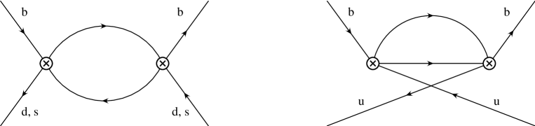
Figure 5: Feynman diagrams entering at the LO in the calculation of the coefficient functions $c^{q}_{k}$ for $q=u,d,s$.

For $q=u$ instead, the relevant one-loop diagram is shown in fig. 5 (right). It gives

$$\begin{array}[]{lll}A^{u}_{1,11}={{\left(1-z\right)}^{2}}\,,&A^{u}_{1,12}={\displaystyle{1\over 3}}\left(1-z\right)^{2}\,,&A^{u}_{1,22}={{\left(1-z\right)}^{2}}\,,\\ A^{u}_{2,11}=0\,,&A^{u}_{2,12}=0\,,&A^{u}_{2,22}=0\,,\\ A^{u}_{3,11}=0\,,&A^{u}_{3,12}=2\,{{\left(1-z\right)}^{2}}\,,&A^{u}_{3,22}=0\,,\\ A^{u}_{4,11}=0\,,&A^{u}_{4,12}=0\,,&A^{u}_{4,22}=0\,.\end{array}$$ (25)

The NLO coefficients $B^{d}_{k,ij}$ are obtained by computing the diagrams shown in figs. 2 and 3. The details of the matching procedure have been discussed in the previous section. We just remind here that we have neglected corrections of ${\cal O}(m_{c}^{2}/m_{b}^{2})$ in the NLO calculation.

At the NLO, the coefficients depend on the renormalization scheme chosen for the HQET operators in eq. (14). We have computed these coefficients in the $\mbox{NDR-}\overline{\rm{MS}}$ scheme defined in ref. [27]. In this scheme, for the coefficients $B^{d}_{k,ij}(\mu)$ we obtain

$$\begin{array}[]{lll}B^{d}_{1,11}=-{{\displaystyle{230\over 81}}}\,,&B^{d}_{1,12}={{\displaystyle{778\over 243}}}+{{\displaystyle{32\,{L}\over 9}}}\,,&B^{d}_{1,22}=-{{\displaystyle{314\over 81}}}+{{\displaystyle{16\,{{\pi}^{2}}\over 27}}}\,,\\ B^{d}_{2,11}=-{{\displaystyle{100\over 81}}}\,,&B^{d}_{2,12}={{\displaystyle{404\over 243}}}+{{\displaystyle{16\,{L}\over 9}}}\,,&B^{d}_{2,22}=-{{\displaystyle{106\over 81}}}+{{\displaystyle{8\,{{\pi}^{2}}\over 27}}}\,,\\ B^{d}_{3,11}={{\displaystyle{925\over 54}}}+18\,{L}\,,&B^{d}_{3,12}={{\displaystyle{2689\over 162}}}+{{\displaystyle{46\,{L}\over 3}}}\,,&B^{d}_{3,22}={{\displaystyle{91\over 9}}}-{{\displaystyle{4\,{{\pi}^{2}}\over 9}}}+8\,{L}\,,\\ B^{d}_{4,11}={{\displaystyle{455\over 54}}}+9\,{L}\,,&B^{d}_{4,12}={{\displaystyle{1337\over 162}}}+{{\displaystyle{23\,{L}\over 3}}}\,,&B^{d}_{4,22}={{\displaystyle{85\over 18}}}-{{\displaystyle{2\,{{\pi}^{2}}\over 9}}}+4\,{L}\,,\end{array}$$ (26)

where $L=\log\left(\mu/m_{b}\right)$. In the case $q=u$, the relevant Feynman diagrams involve gluon corrections to the LO diagram shown on the right side of fig. 5. We obtain for the coefficients

$$\begin{array}[]{ll}B^{u}_{1,11}={{\displaystyle{188\over 27}}}-{{\displaystyle{16\,{{\pi}^{2}}\over 9}}}\,,&B^{u}_{1,12}=-{{\displaystyle{1312\over 81}}}-{{\displaystyle{32\,{{\pi}^{2}}\over 27}}}-{{\displaystyle{32\,{L}\over 3}}}\,,\\ B^{u}_{1,22}={{\displaystyle{188\over 27}}}-{{\displaystyle{16\,{{\pi}^{2}}\over 9}}}\,,&B^{u}_{2,11}={{\displaystyle{16\over 27}}}\,,\\ B^{u}_{2,12}=-{{\displaystyle{32\over 81}}}\,,&B^{u}_{2,22}={{\displaystyle{16\over 27}}}\,,\\ B^{u}_{3,11}=-{{\displaystyle{125\over 3}}}-{{\displaystyle{4\,{{\pi}^{2}}\over 3}}}-24\,{L}\,,&B^{u}_{3,12}=-{{\displaystyle{374\over 27}}}-{{\displaystyle{28\,{{\pi}^{2}}\over 9}}}-10\,{L}\,,\\ B^{u}_{3,22}=-{{\displaystyle{125\over 3}}}-{{\displaystyle{4\,{{\pi}^{2}}\over 3}}}-24\,{L}\,,&B^{u}_{4,11}=-{{\displaystyle{4\over 3}}}\,,\\ B^{u}_{4,12}=-{{\displaystyle{100\over 27}}}\,,&B^{u}_{4,22}=-{{\displaystyle{4\over 3}}}\,.\end{array}$$ (27)

	$q=d$		$q=u$		$q=s$
	LO	NLO	LO	NLO	LO	NLO
$c^{q}_{1}$	$-0.32$	$-0.30$	$0.92$	$0.90$	$-0.27$	$-0.25$
$c^{q}_{2}$	$-0.18$	$-0.16$	$0.00$	$0.02$	$-0.17$	$-0.15$
$c^{q}_{3}$	$0.20$	$0.16$	$-0.83$	$-1.42$	$0.17$	$0.13$
$c^{q}_{4}$	$0.11$	$0.08$	$0.00$	$0.00$	$0.11$	$0.08$
$\widetilde{c}^{\,q}_{1}$	$-0.02$	$-0.03$	$-0.06$	$-0.33$	$-0.01$	$-0.03$
$\widetilde{c}^{\,q}_{2}$	$0.02$	$0.03$	$0.00$	$-0.01$	$0.02$	$0.03$
$\widetilde{c}^{\,q}_{3}$	$-0.70$	$-0.65$	$2.11$	$2.27$	$-0.60$	$-0.54$
$\widetilde{c}^{\,q}_{4}$	$0.79$	$0.68$	$0.00$	$-0.06$	$0.77$	$0.65$

Table 1: Wilson coefficients $c^{q}_{k}$ computed at the LO and NLO ($\overline{\rm MS}$ scheme). As reference values, we use $\mu=m_{b}=4.8$ GeV and $m_{c}=1.4$ GeV. The coefficients $\widetilde{c}^{q}_{k}$ in the operator basis of eq. (40) are also shown.

Finally, we discuss the extension of eq. (21) to the case $q=s$. With respect to $c^{d}_{k}(\mu)$, the coefficient functions $c^{s}_{k}(\mu)$ receive, at the NLO, additional contributions coming from the penguin contraction of the current-current operators (diagram $D_{13}$ of fig. 2) and from the insertion of penguin and chromomagnetic operators (diagram $D_{14}$ of fig. 2). Since the Wilson coefficients $C_{3}$–$C_{6}$ are small, contributions with a double insertion of penguin operators can be safely neglected. As suggested in [35], a consistent way for implementing this approximation is to consider the coefficients $C_{3}$–$C_{6}$ as formally of ${\cal O}(\alpha_{s})$. Within this approximation, only single insertions of penguin operators need to be considered at the NLO. Therefore we can write

$$c^{s}_{k}(\mu) = c^{d}_{k}(\mu)+\frac{\alpha_{s}}{4\pi}\,C_{2}(\mu)^{2}\,P_{k,22}(\mu)+2\frac{\alpha_{s}}{4\pi}C_{2}(\mu)C_{8G}(\mu)P_{k,28}(\mu)+$$ (28)

$$2\mathop{\displaystyle\sum}_{i=1,2}\mathop{\displaystyle\sum}_{r=3,4}C_{i}(\mu)\,C_{r}(\mu)P_{k,ir}(\mu)\,,$$

and we obtain

$$\begin{array}[]{ll}P_{1,22}={\displaystyle{32\over 243}}+{\displaystyle{32\,{L}\over 81}}\,,&P_{2,22}={\displaystyle{16\over 243}}+{\displaystyle{16\,{L}\over 81}}\,,\\ P_{3,22}=-{\displaystyle{8\over 81}}-{\displaystyle{8\,{L}\over 27}}\,,&P_{4,22}=-{\displaystyle{4\over 81}}-{\displaystyle{4\,{L}\over 27}}\,,\end{array}$$ (29)

$$\begin{array}[]{llll}P_{1,13}=-{\displaystyle{1\over 3}}\,,&P_{2,13}=-{\displaystyle{1\over 6}}\,,&P_{3,13}=-2\,,&P_{4,13}=-1\,,\\ P_{1,14}=-{\displaystyle{1\over 9}}\,,&P_{2,14}=-{\displaystyle{1\over 18}}\,,&P_{3,14}=-{\displaystyle{2\over 3}}\,,&P_{4,14}=-{\displaystyle{1\over 3}}\,,\\ P_{1,23}=-{\displaystyle{1\over 9}}\,,&P_{2,23}=-{\displaystyle{1\over 18}}\,,&P_{3,23}=-{\displaystyle{2\over 3}}\,,&P_{4,23}=-{\displaystyle{1\over 3}}\,,\\ P_{1,24}=-{\displaystyle{1\over 3}}\,,&P_{2,24}=-{\displaystyle{1\over 6}}\,,&P_{3,24}=0\,,&P_{4,24}=0\,,\\ P_{1,28}=-{\displaystyle{8\over 27}}\,,&P_{2,28}=-{\displaystyle{4\over 27}}\,,&P_{3,28}={\displaystyle{2\over 9}}\,,&P_{4,28}={\displaystyle{1\over 9}}\,.\end{array}$$ (30)

The coefficients $P_{k,28}$ are computed using the convention in which the chromomagnetic coefficient $C_{8}$ has a positive sign. The NLO contribution of penguin and chromomagnetic operators to beauty hadron lifetimes has been also computed in ref. [36]. We verified that our results are in agreement with them.

For convenience, we present in table 1 the numerical values of the coefficients $c_{k}^{q}(\mu)$, in the cases $q=u,d,s$, at $\mu=m_{b}=4.8$ GeV, both at LO and NLO. We also give the coefficients $\widetilde{c}_{k}^{q}(\mu)$ defined in the operator basis of ref. [7]. For details on the conversion between the two basis, see sect. 6.1

5 Matching of $\Delta B=0$ non-singlet operators between QCD and HQET

Theoretical predictions of beauty hadron lifetimes, based on the OPE, are obtained by combining the perturbative determination of the Wilson coefficients with the non-perturbative evaluation of the hadronic matrix elements of the HQET operators. In the next section, we will perform a phenomenological analysis, by using the NLO results for the Wilson coefficients and the lattice determinations of the relevant hadronic matrix elements. In some cases the lattice results are provided in terms of matrix elements of QCD operators. In order to use these determinations, consistently at the NLO, it is necessary to perform an additional matching between the QCD and the HQET operators. For the dimension-six $\Delta B=0$ operators of interest in this paper, this matching has not been computed so far. For this reason, we present in this section the results of an ${\cal O}(\alpha_{s})$ calculation of the coefficient functions relating the QCD four-fermion $\Delta B=0$ operators to their counterparts in HQET.

We limit ourselves to the case of flavour non-singlet operators, which are the only ones for which lattice results are available so far. An important example is the difference $O^{u}_{k}-O^{d}_{k}$ of the operators defined in eq. (14) which determines, as we will see below, the lifetime ratio of charged to neutral $B$ mesons. In the limit of exact flavour symmetry, these operators do not mix with lower dimensional operators. For this reason, their matching between QCD and HQET does not require the calculation of penguin contractions and only involves current-current operators of dimension six.

The matching equation between the operators in QCD and HQET can be written in the form

$${\vec{O}}_{\rm QCD}(\mu)=\widehat{C}(\mu,\mu^{\prime},m_{b})\,{\vec{O}}_{\rm HQET}(\mu^{\prime})\,.$$ (31)

The scale dependence of the coefficient functions $\widehat{C}(\mu,\mu^{\prime},m_{b})$ is governed by the renormalization group equation of the QCD and HQET operators respectively. Thus one finds

$$\widehat{C}(\mu,\mu^{\prime},m_{b})=\left(W(\mu,m_{b})^{T}\right)^{-1}\widehat{C}(m_{b})\,\widetilde{W}(\mu^{\prime},m_{b})^{T}$$ (32)

where the matrix $W(\mu,m_{b})$ in QCD is given, at the NLO, by

$$W(\mu,m_{b})=\left(1+\frac{\alpha_{s}(\mu)}{4\pi}J(\mu)\right)\left(\frac{\alpha_{s}(\mu)}{\alpha_{s}(m_{b})}\right)^{-\gamma_{0}^{T}/2\beta_{0}}\left(1-\frac{\alpha_{s}(m_{b})}{4\pi}J(m_{b})\right)$$ (33)

and $\widetilde{W}(\mu,m_{b})$ is its analogous in the HQET. For convenience, we present here the expressions of the leading anomalous dimension matrices, $\gamma_{0}$ and $\widetilde{\gamma}_{0}$ in QCD and HQET. In the basis of eq. (14) they reads [37, 38]

$$\gamma_{0}=\left(\begin{array}[]{cccc}0&0&12&0\cr 0&0&0&-12\cr 8/3&0&-4&0\cr 0&-8/3&0&-14\cr\end{array}\right)\,,\qquad\widetilde{\gamma}_{0}=\left(\begin{array}[]{cccc}0&0&0&0\cr 0&0&0&0\cr 0&0&-9&0\cr 0&0&0&-9\cr\end{array}\right)\,.$$ (34)

The matrix $J$, in eq. (33), is expressed in terms of the two-loop anomalous dimension, and it is defined for instance in ref. [34]. In the case of the HQET, the NLO anomalous dimension is still unknown.

The matrix $\widehat{C}(m_{b})$ is the coefficient function at the matching scales $\mu=\mu^{\prime}=m_{b}$. At the NLO, it can be written in the form:

$$\widehat{C}(m_{b})=1+\frac{\alpha_{s}(m_{b})}{4\pi}\,\widehat{C}_{1}\,.$$ (35)

We have computed $\widehat{C}_{1}$ considering two different renormalization schemes for the QCD operators, namely $\mbox{NDR-}\overline{\rm{MS}}$ and Landau RI-MOM (see ref. [34] for a detailed definitions of these schemes). The HQET operators are renormalized in the $\mbox{NDR-}\overline{\rm{MS}}$ scheme of ref. [27]. By denoting the results with $\widehat{C}_{1}^{\overline{\rm{MS}}}$ and $\widehat{C}_{1}^{\rm RI}$ respectively, in the operator basis of eq. (14), we obtain:

$$\widehat{C}_{1}^{\overline{\rm{MS}}}=\left(\begin{array}[]{cccc}-4/3&4/3&-18&-2\cr 4/3&-4/3&2&6\cr-4&-4/9&-35/6&-5/2\cr 4/9&4/3&-5/6&25/6\cr\end{array}\right)$$ (36)

and

$$\widehat{C}_{1}^{\rm RI}=\left(\begin{array}[]{cccc}-4/3&4/3&-4-24\,{\log 2}&-2\cr 4/3&-4/3&2&2-4\,{\log 2}\cr-8/9-16/3\,{\log 2}&-4/9&-21/2+8\,{\log 2}&-5/2\cr 4/9&4/9-8/9\,{\log 2}&-5/6&-13/2+4/3\,{\log 2}\cr\end{array}\right)\,.$$ (37)

Note that the difference $C_{1}^{\overline{\rm{MS}}}-C_{1}^{\rm RI}$ is the one loop matrix which provides the connection between the $\overline{\rm{MS}}$ and $\rm RI$ schemes in QCD for the $\Delta B=0$ operators. We have checked that this matrix agrees with the matrix denoted as $\hat{r}_{\overline{\rm{MS}}}$ in ref. [34], once the proper change of basis is performed.

In the next section, the matrix $C_{1}^{\overline{\rm{MS}}}$ of eq. (36) will be used to convert the lattice results for the matrix elements of the QCD operators into their HQET counterparts.

6 Phenomenological Discussion

In this section we perform a phenomenological analysis of the lifetime ratios of beauty hadrons, by using the NLO expressions of the Wilson coefficients and the lattice determinations of the relevant hadronic matrix elements [9]-[12].

The starting point of this analysis is eq. (13), which expresses the ratio of inclusive widths of beauty hadrons, up to and including $1/m_{b}^{3}$ spectator effects. The combinations of hadronic parameters entering this formula at order $1/m_{b}^{2}$ can be evaluated from the heavy hadron spectroscopy [39]. The numerical contributions of these terms to the lifetime ratios are rather small, and one obtains the estimate

$${\displaystyle{\tau(B^{+})\over\tau(B_{d})}}=1.00-\Delta^{B^{+}}_{\rm\scriptstyle spec}\,,\quad{\displaystyle{\tau(B_{s})\over\tau(B_{d})}}=1.00-\Delta^{B_{s}}_{\rm\scriptstyle spec}\,,\quad{\displaystyle{\tau(\Lambda_{b})\over\tau(B_{d})}}=0.98(1)-\Delta^{\Lambda}_{\rm\scriptstyle spec}\,,$$ (38)

which can be compared with the experimental results in eq. (2). In the previous expressions the $\Delta$s represent the $1/m_{b}^{3}$ contributions of hard spectator effects

$$\Delta^{H_{b}}={\displaystyle{96\pi^{2}\over m_{b}^{3}\,c^{(3)}}}\mathop{\displaystyle\sum}\limits_{k}c^{(6)}_{k}\left(\frac{\langle O^{(6)}_{k}\rangle_{H_{b}}}{2M_{H_{b}}}-\frac{\langle O_{k}^{(6)}\rangle_{B_{d}}}{2M_{B_{d}}}\right)\,.$$ (39)

These are the quantities which we are interested in. They are expressed in terms of coefficient functions and matrix elements of dimension-six operators. In the phenomenological analysis, we use the non-perturbative determination of the relevant matrix elements from lattice QCD calculation. For recent estimates based on QCD sum rules, see refs. [40]–[43].

6.1 Matrix Elements

The basis of four-fermion operators usually considered in the literature to study the lifetime ratios of beauty hadrons is given by [7]

$$\begin{array}[]{ll}{\cal O}^{q}_{1}=(\bar{b}_{i}q_{i})_{V-A}\,(\bar{q}_{j}b_{j})_{V-A}\,,&{\cal O}^{q}_{2}=(\bar{b}_{i}q_{i})_{S-P}\,(\bar{q}_{j}b_{j})_{S+P}\,,\\ {\cal O}^{q}_{3}=(\bar{b}_{i}t^{a}_{ij}q_{j})_{V-A}\,(\bar{q}_{k}t^{a}_{kl}b_{l})_{V-A}\,,&{\cal O}^{q}_{4}=(\bar{b}_{i}t^{a}_{ij}q_{j})_{S-P}\,(\bar{q}_{k}t^{a}_{kl}b_{l})_{S+P}\,,\end{array}$$ (40)

where $q=u,d,s,c$ and $(\bar{q}q)_{S\pm P}=\bar{q}(1\pm\gamma^{5})q$. In this basis, which differs from the one in eq. (14) by a Fierz rearrangement, the matrix elements of the operators ${\cal O}^{q}_{3}$ and ${\cal O}^{q}_{4}$, between external $B$-mesons states, vanish in the vacuum saturation approximation (VSA). By following the convention adopted in the literature, we will work in this section in the basis of eq. (40), to which we add the penguin operator of eq. (15). The Wilson coefficients associated to the new basis will be indicated by the symbol $\widetilde{c}_{k}^{\,q}$. They are related to those defined in the previous sections by a linear transformation

$$\widetilde{c}_{k}^{\,q}=M_{kj}c_{j}^{q}\,,\qquad M=\left(\begin{array}[]{cccc}1/3&0&4/9&0\cr 0&-2/3&0&-8/9\cr 2&0&-1/3&0\cr 0&-4&0&2/3\cr\end{array}\right)\,.$$ (41)

The values of $\widetilde{c}_{k}^{\,q}$ at $\mu=m_{b}$ are given in table 1.

In parametrizing the matrix elements of the current-current operators, it is useful to distinguish two cases, depending on whether or not the light quark $q$ of the operator enters as a valence quark in the external hadronic state. From a diagrammatic point of view, this difference gives rise to a different number of Wick contractions. In the case of external $B$-meson states, for instance, the matrix elements of the valence operators are computed by evaluating non-perturbatively the two Feynman diagrams shown in fig. 6, while for non-valence operators only the second diagram appears.

Figure 6: Feynman diagrams entering the non-perturbative evaluation of the matrix elements of valence operators between external $B$-meson states. In the case of non-valence operators only the second diagram appears.

We find it convenient to introduce different $B$-parameters for the valence and non-valence contributions. Thus, for the $B$-meson matrix elements of the non-valence operator we define

$${\displaystyle{\langle B_{q}|{\cal O}^{q^{\prime}}_{k}|B_{q}\rangle\over 2M_{B_{q}}}}={\displaystyle{f_{B_{q}}^{2}M_{B_{q}}\over 2}}\,\delta_{k}^{\,q^{\prime}q}\quad{\rm for}\,\,q\neq q^{\prime}\,,$$ (42)

and, for the valence operators ($q=q^{\prime}$), we write

$$\begin{array}[]{ll}{\displaystyle{\langle B_{q}|{\cal O}^{q}_{1}|B_{q}\rangle\over 2M_{B_{q}}}}={\displaystyle{f_{B_{q}}^{2}M_{B_{q}}\over 2}}\,\left(B_{1}^{\,q}+\delta_{1}^{\,qq}\right)\,,\quad{\displaystyle{\langle B_{q}|{\cal O}^{q}_{3}|B_{q}\rangle\over 2M_{B_{q}}}}={\displaystyle{f_{B_{q}}^{2}M_{B_{q}}\over 2}}\,\left(\varepsilon_{1}^{\,q}+\delta_{3}^{\,qq}\right)\,,\\ {\displaystyle{\langle B_{q}|{\cal O}^{q}_{2}|B_{q}\rangle\over 2M_{B_{q}}}}={\displaystyle{f_{B_{q}}^{2}M_{B_{q}}\over 2}}\,\left(B_{2}^{\,q}+\delta_{2}^{\,qq}\right)\,,\quad{\displaystyle{\langle B_{q}|{\cal O}^{q}_{4}|B_{q}\rangle\over 2M_{B_{q}}}}={\displaystyle{f_{B_{q}}^{2}M_{B_{q}}\over 2}}\,\left(\varepsilon_{2}^{\,q}+\delta_{4}^{\,qq}\right)\,.\end{array}$$ (43)

In eq. (43), the $\delta_{k}^{\,qq}$ are defined as the parameters $\delta_{k}^{\,qq^{\prime}}$ of eq. (42) in the limit of degenerate quark masses ($m_{q}=m_{q^{\prime}}$). In the VSA, $B_{1}^{\,q}=B_{2}^{\,q}=1$ while the $\varepsilon$ parameters and all the $\delta$s vanish. It should be clear that the $B_{k}$, $\varepsilon_{k}$ and $\delta_{k}$ have a direct interpretation in terms of Feynman diagrams, and are represented by the first ($B_{k}$, $\varepsilon_{k}$) and second ($\delta_{k}$) contraction of fig. 6 respectively. Each of these parameters is a well defined and gauge invariant quantity. In the exact $SU(2)$ limit, for instance, the parameters $B_{k}^{\,d}$ express the matrix elements of the non-singlet operator $O^{u}_{k}-O^{d}_{k}$ between external $B$-meson states.

Our definition of $B_{1}$, $B_{2}$, $\varepsilon_{1}$ and $\varepsilon_{2}$ differs from the one considered in the literature for the presence of the $\delta$s in eq. (43). The reason why we have distinguished between valence and non valence contributions, in these definitions, is that lattice QCD calculations [9]-[12] have not computed, so far, the full matrix elements, but only the valence contributions represented the first diagram of fig. 6. Thus, the $B_{k}$ and $\varepsilon_{k}$ parameters, defined as in eq. (43), denote the quantities actually determined, at present, by lattice calculations. In principle, a non-perturbative calculation of the $\delta$ parameters on the lattice is possible. However, it requires dealing with the difficult problem of power-divergence subtractions which has prevented so far the calculation of the corresponding diagrams.

To complete the definitions of the $B$-parameters for the $B$-mesons, we introduce a parameter for the matrix element of the penguin operator

$${\displaystyle{\langle B_{q}|O_{P}|B_{q}\rangle\over 2M_{B_{q}}}}={\displaystyle{f_{B}^{2}M_{B}\over 2}}\,P^{\,q}\,.$$ (44)

We now define the $B$-parameters for the $\Lambda_{b}$ baryon. Up to $1/m_{b}$ corrections, the matrix elements of the operators ${\cal O}^{q}_{2}$ and ${\cal O}^{q}_{4}$, between external $\Lambda_{b}$ states, can be related to the matrix elements of the operators ${\cal O}^{q}_{1}$ and ${\cal O}^{q}_{3}$ [7]

$$\langle\Lambda_{b}|{\cal O}^{q}_{1}|\Lambda_{b}\rangle=-2\,\langle\Lambda_{b}|{\cal O}^{q}_{2}|\Lambda_{b}\rangle\,,\quad\langle\Lambda_{b}|{\cal O}^{q}_{3}|\Lambda_{b}\rangle=-2\,\langle\Lambda_{b}|{\cal O}^{q}_{4}|\Lambda_{b}\rangle\,.$$ (45)

For the independent matrix elements, assuming $SU(2)$ symmetry, we define

$${\displaystyle{\langle\Lambda_{b}|{\cal O}^{q}_{1}|\Lambda_{b}\rangle\over 2M_{\Lambda_{b}}}}={\displaystyle{f_{B}^{2}M_{B}\over 2}}\,\left(L_{1}+\delta_{1}^{\,\Lambda q}\right)\quad{\rm for}\,\,q=u,d\,,$$

$${\displaystyle{\langle\Lambda_{b}|{\cal O}^{q}_{3}|\Lambda_{b}\rangle\over 2M_{\Lambda_{b}}}}={\displaystyle{f_{B}^{2}M_{B}\over 2}}\,\left(L_{2}+\delta_{2}^{\,\Lambda q}\right)\quad{\rm for}\,\,q=u,d\,,$$

$${\displaystyle{\langle\Lambda_{b}|{\cal O}^{q}_{1}|\Lambda_{b}\rangle\over 2M_{\Lambda_{b}}}}={\displaystyle{f_{B}^{2}M_{B}\over 2}}\,\delta_{1}^{\,\Lambda q}\quad{\rm for}\,\,q=s,c\,,$$ (46)

$${\displaystyle{\langle\Lambda_{b}|{\cal O}^{q}_{3}|\Lambda_{b}\rangle\over 2M_{\Lambda_{b}}}}={\displaystyle{f_{B}^{2}M_{B}\over 2}}\,\delta_{2}^{\,\Lambda q}\quad{\rm for}\,\,q=s,c\,,$$

$${\displaystyle{\langle\Lambda_{b}|O_{P}|\Lambda_{b}\rangle\over 2M_{\Lambda_{b}}}}={\displaystyle{f_{B}^{2}M_{B}\over 2}}\,P^{\,\Lambda}\,.$$

In analogy with the $B$-meson case, the parameters $L_{1}$ and $L_{2}$ represent the valence contributions computed by current lattice calculations [10, 11].

At present, two independent lattice calculations of the $B$-parameters in the $B$-meson sector have been performed, both in the quenched approximation. In the first study [9, 11], the parameters $B_{1}^{d}$, $B_{2}^{d}$, $\varepsilon_{1}^{d}$ and $\varepsilon_{2}^{d}$ have been computed by simulating on the lattice the HQET. The second calculation [12], instead, has been performed by using QCD, and the results have been obtained in this case for both $B_{u,d}$ and $B_{s}$ mesons. The calculation of ref.[12] is also accurate at the NLO, since the $B$-parameters have been evolved, from the lattice scale up to $m_{b}$, by using the two-loop anomalous dimension of the four-fermion $\Delta B=0$ operators, which is known in QCD [34, 44], but not in the HQET. For these reasons, we will use the results of ref. [12] in our phenomenological analysis. The parameters $B_{1}^{q}$, $B_{2}^{q}$, $\varepsilon_{1}^{q}$ and $\varepsilon_{2}^{q}$, computed in QCD, have been matched from QCD to HQET, at the NLO, using the coefficients presented in the previous section, eqs. (35)-(36). After applying these coefficients to the QCD lattice results of ref. [12], we obtain the estimates of the HQET $B$-parameters collected in table 2.

$B_{1}^{d}$ = $1.2\pm 0.2$	$B_{1}^{s}$ = $1.0\pm 0.1$
$B_{2}^{d}$ = $0.7\pm 0.1$	$B_{2}^{s}$ = $0.7\pm 0.1$
$\varepsilon_{1}^{d}$ = $0.03\pm 0.02$	$\varepsilon_{1}^{s}$ = $0.03\pm 0.01$
$\varepsilon_{2}^{d}$ = $0.04\pm 0.01$	$\varepsilon_{2}^{s}$ = $0.03\pm 0.01$
$L_{1}$ = $-0.2\pm 0.1$	$L_{2}$ = $0.2\pm 0.1$
$m_{b}$ = $4.8\pm 0.1$ GeV	$m_{b}-m_{c}$ = $3.40\pm 0.06$ GeV
$f_{B}$ = $200\pm 25$ MeV	$f_{B_{s}}/f_{B}$ = $1.16\pm 0.04$

Table 2: Central values and standard deviations of the input parameters used in the numerical analysis.

For comparison, we also present here the values of $B$-parameters obtained in ref. [9, 11] from the lattice simulation in the HQET. In this case, a different definition of the $\overline{\rm{MS}}$ scheme has been adopted. The NLO connection between this scheme and the one of ref. [27], chosen in this paper, is given by [45]

$$\left(\begin{array}[]{c}B_{2}^{q}\cr\varepsilon_{2}^{q}\end{array}\right)=\left[1+\frac{\alpha_{s}}{4\pi}\left(\begin{array}[]{cc}0&-3/2\cr-1/3&-7/4\end{array}\right)\right]\left(\begin{array}[]{c}B_{2}^{q}\cr\varepsilon_{2}^{q}\end{array}\right)_{\rm SDP}$$ (47)

where the label SDP denotes the parameters in the scheme of ref. [9]. The other parameters, $B_{1}^{q}$ and $\varepsilon_{1}^{q}$, are the same in both schemes. After applying eq. (47), the results of refs. [9, 11] read

$$B^{d}_{1}=1.06\pm 0.08\,,\quad B^{d}_{2}=1.01\pm 0.07\,,$$

$$\varepsilon^{d}_{1}=-0.01\pm 0.03\,,\quad\varepsilon^{d}_{2}=-0.03\pm 0.02\,.$$ (48)

The differences between these results and those given in table 2 may give an estimate of the higher orders $1/m_{b}$ corrections neglected in the static calculation of ref. [9, 11], and of the systematic uncertainty introduced by the large extrapolation in the $b$-quark mass performed in ref. [12]. It should be also kept in mind, however, that the renormalization group evolution has been only performed in ref. [9, 11] with a LO accuracy.

For the $\Lambda_{b}$ baryon, only the non-perturbative results of an exploratory study in the HQET are available at present [10]. They have been obtained with a LO accuracy, at a rather large value of the lattice spacing and do not include the extrapolation of the light quark masses to their physical values. For these reasons, in quoting the values of the corresponding $B$ parameters, $L_{1}$ and $L_{2}$ in table 2, we also include in the error our estimate of the remaining systematic uncertainties. We also note that, in all these calculations, the matching between the lattice and the continuum theory has been performed using 1-loop perturbation theory, and that the leading perturbative corrections are typically found to be large. For this reason, a non-perturbative evaluation of the relevant renormalization constants would be very interesting. For $B$ mesons, such a calculation is in progress [46].

For the large number of $\delta$ and $P$ parameters in eqs. (42)-(6.1), which define the non-valence contributions and the matrix elements of the penguin operator, only phenomenological estimates exist [38, 47]. These estimates indicate that the matrix elements of non-valence operators are suppressed, with respect to the valence ones, by at least one order of magnitude. These contributions cancel out in the theoretical evaluation of the lifetime ratio $\tau(B^{+})/\tau(B_{d})$, see eq. (6.2), while they enter the determination of $\tau(\Lambda_{b})/\tau(B_{d})$ and $\tau(B_{s})/\tau(B_{d})$, the latter for $SU(3)$ breaking effects. Lacking quantitative calculations of the $\delta$ and $P$ parameters, we will mainly rely in our numerical analysis on the results of the phenomenological estimates, and neglect these contributions. A qualitative estimate of the error introduced by this approximation in the case of the ratio $\tau(\Lambda_{b})/\tau(B_{d})$ will be given at the end of the section.

6.2 Results

We now present the detailed expressions of the spectator contributions, represented, in eq. (39), by the quantities $\Delta_{spec}$. In these expressions all terms, coming from both valence and non-valence contributions, which are often omitted in the literature, will be explicitly taken into account. Using eq. (38), and the definitions of the $B$-parameters in eqs. (42)-(6.1), the spectator contributions take the following expressions

$$\Delta^{B^{+}}_{\rm\scriptstyle spec} = 48\pi^{2}\,\frac{f_{B}^{2}M_{B}}{m_{b}^{3}c^{(3)}}\,\mathop{\displaystyle\sum}_{k=1}^{4}\left(\widetilde{c}_{k}^{\,u}-\widetilde{c}_{k}^{\,d}\right){\cal B}_{k}^{\,d}\,,$$

$$\Delta^{B_{s}}_{\rm\scriptstyle spec} = 48\pi^{2}\,\frac{f_{B}^{2}M_{B}}{m_{b}^{3}c^{(3)}}\,\left\{\mathop{\displaystyle\sum}_{k=1}^{4}\left[r\,\widetilde{c}_{k}^{\,s}\,{\cal B}_{k}^{\,s}-\widetilde{c}_{k}^{\,d}\,{\cal B}_{k}^{\,d}+\left(\widetilde{c}_{k}^{\,u}+\widetilde{c}_{k}^{\,d}\right)\left(r\,\delta_{k}^{\,ds}-\delta_{k}^{\,dd}\right)+\right.\right.$$ (49)

$$\qquad\qquad\quad\left.\left.\widetilde{c}_{k}^{\,s}\left(r\,\delta_{k}^{\,ss}-\delta_{k}^{\,sd}\right)+\widetilde{c}_{k}^{\,c}\left(r\,\delta_{k}^{\,cs}-\delta_{k}^{\,cd}\right)\right]+c_{P}\left(rP^{\,s}-P^{\,d}\right)\right\}\,,$$

$$\Delta^{\Lambda}_{\rm\scriptstyle spec} = 48\pi^{2}\,\frac{f_{B}^{2}M_{B}}{m_{b}^{3}c^{(3)}}\,\left\{\mathop{\displaystyle\sum}_{k=1}^{4}\left[\left(\widetilde{c}_{k}^{\,u}+\widetilde{c}_{k}^{\,d}\right){\cal L}_{k}^{\,\Lambda}-\widetilde{c}_{k}^{\,d}\,{\cal B}_{k}^{\,d}+\left(\widetilde{c}_{k}^{\,u}+\widetilde{c}_{k}^{\,d}\right)\left(d_{k}^{\,\Lambda d}-\delta_{k}^{\,dd}\right)+\right.\right.$$

$$\qquad\qquad\quad\left.\left.\widetilde{c}_{k}^{\,s}\left(d_{k}^{\,\Lambda s}-\delta_{k}^{\,sd}\right)+\widetilde{c}_{k}^{\,c}\left(d_{k}^{\,\Lambda c}-\delta_{k}^{\,cd}\right)\right]+c_{P}\left(P^{\,\Lambda}-P^{\,d}\right)\right\}\,.$$

The $\widetilde{c}_{k}$ are the coefficient functions given in eq. (41). The factor $r$ denotes the ratio $(f_{B_{s}}^{2}M_{B_{s}})/(f_{B}^{2}M_{B})$ and, in order to simplify the notation, we have defined the vectors of parameters

$$\vec{\cal B}^{q}=\{B_{1}^{q},B_{2}^{q},\varepsilon_{1}^{q},\varepsilon_{1}^{q}\}\,,$$

$$\vec{\cal L}=\{L_{1},-L_{1}/2,L_{2},-L_{2}/2\}\,,$$ (50)

$$\vec{d}^{\Lambda q}=\{\delta^{\Lambda q}_{1},-\delta^{\Lambda q}_{1}/2,\delta^{\Lambda q}_{2},-\delta^{\Lambda q}_{2}/2\}\,.$$

Because of the $SU(2)$ symmetry, the non-valence and penguin contributions cancel out in the expressions of the lifetime ratio $\tau(B^{+})/\tau(B_{d})$. From this point of view, the theoretical prediction of this ratio is at present the most accurate, since it depends only on the non-perturbative parameters actually computed by current lattice calculations. The prediction of the ratio $\tau(\Lambda_{b})/\tau(B_{d})$, instead, is affected by both the uncertainties on the values of the $\delta$ and $P$ parameters, and by the unknown expressions of the Wilson coefficients $\widetilde{c}_{k}^{\,c}$ and $c_{P}$ at the NLO. For the ratio $\tau(B_{s})/\tau(B_{d})$ the same uncertainties exists. However they are expected to be smaller, since these contributions cancel in the limit of exact $SU(3)$ symmetry.

In order to evaluate the lifetime ratios, we have performed a Monte Carlo calculation, by extracting the input parameters with flat distributions with central values and standard deviations given in table 2. The contributions of all the $\delta$ and $P$ parameters have been neglected. The strong coupling constant has been kept fixed at the value $\alpha_{s}(m_{b})=0.214$. The values of the bottom and charm quark masses, given in the table and used in the numerical analysis, correspond to the pole mass definition. The parameter $c^{(3)}$ in eq. (6.2) is a function of the ratio $m_{c}^{2}/m_{b}^{2}$, and such a dependence has been consistently taken into account in the numerical analysis. For the range of masses given in table 2, $c^{(3)}$ varies in the interval $c^{(3)}=3.4\div 4.2$ [20]-[22].

For convenience, we also present the numerical expression corresponding to eq. (6.2), by omitting the non valence and penguin contributions. We find

$$\left.\begin{array}[]{ll}\Delta^{B^{+}}_{\rm\scriptstyle spec}\,=&-\,0.011(3)\,B_{1}^{d}-0.005(1)\,B_{2}^{d}+0.7(2)\,\varepsilon_{1}^{d}-0.19(5)\,\varepsilon_{2}^{d}\,,\\ \\ \Delta^{B_{s}}_{\rm\scriptstyle spec}\,=&-\,0.004(1)\,B_{1}^{s}+0.005(1)\,B_{2}^{s}-0.17(4)\,\varepsilon_{1}^{s}+0.22(6)\,\varepsilon_{2}^{s}\\ &+\,0.004(1)\,B_{1}^{d}-0.005(1)\,B_{2}^{d}+0.17(4)\,\varepsilon_{1}^{d}-0.19(5)\,\varepsilon_{2}^{d}\,,\\ \\ \Delta^{\Lambda}_{\rm\scriptstyle spec}\,=&-\,0.022(6)\,L_{1}+0.24(6)\,L_{2}\\ &+\,0.004(1)\,B_{1}^{d}-0.005(1)\,B_{2}^{d}+0.17(4)\,\varepsilon_{1}^{d}-0.19(5)\,\varepsilon_{2}^{d}\,,\end{array}\,\,\,\right\}\,{\rm LO}$$ (51)

at the LO ($\mu=m_{b}$), and

$$\left.\begin{array}[]{ll}\Delta^{B^{+}}_{\rm\scriptstyle spec}\,=&-\,0.07(2)\,B_{1}^{d}-0.011(3)\,B_{2}^{d}+0.7(2)\,\varepsilon_{1}^{d}-0.18(5)\,\varepsilon_{2}^{d}\,,\\ \\ \Delta^{B_{s}}_{\rm\scriptstyle spec}\,=&-\,0.007(2)\,B_{1}^{s}+0.009(2)\,B_{2}^{s}-0.16(4)\,\varepsilon_{1}^{s}+0.20(5)\,\varepsilon_{2}^{s}\\ &+\,0.007(2)\,B_{1}^{d}-0.008(2)\,B_{2}^{d}+0.16(4)\,\varepsilon_{1}^{d}-0.16(4)\,\varepsilon_{2}^{d}\,,\\ \\ \Delta^{\Lambda}_{\rm\scriptstyle spec}\,=&-\,0.09(2)\,L_{1}+0.32(8)\,L_{2}\\ &+\,0.007(2)\,B_{1}^{d}-0.008(2)\,B_{2}^{d}+0.16(4)\,\varepsilon_{1}^{d}-0.16(4)\,\varepsilon_{2}^{d}\,,\end{array}\,\,\,\right\}\,{\rm NLO}$$ (52)

at the NLO. Note that we have shown, for each coefficient, an estimate of the error. These errors, however, are strictly correlated. For this reason, eqs. (51) and (52) have not been used in the numerical analysis.

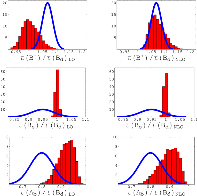
Figure 7: Theoretical (histogram) vs experimental (solid line) distributions of lifetime ratios. The theoretical predictions are shown at the LO (left) and NLO (right).

We finally present our predictions for the lifetimes ratios of beauty hadrons, which have also been quoted in the introduction. Using the LO expressions of the Wilson coefficients, we obtain

$$\left.\frac{\tau(B^{+})}{\tau(B_{d})}\,\right|_{\rm LO}\!\!\!\!\!=1.01\pm 0.03\,,\qquad\left.\frac{\tau(B_{s})}{\tau(B_{d})}\,\right|_{\rm LO}\!\!\!\!\!=1.00\pm 0.01\,,\qquad\left.\frac{\tau(\Lambda_{b})}{\tau(B_{d})}\,\right|_{\rm LO}\!\!\!\!\!=0.93\pm 0.04\,,$$ (53)

while, including the NLO corrections computed in this paper, we get

$$\left.\frac{\tau(B^{+})}{\tau(B_{d})}\,\right|_{\rm NLO}\!\!\!\!\!=1.07\pm 0.03\,,\qquad\left.\frac{\tau(B_{s})}{\tau(B_{d})}\,\right|_{\rm NLO}\!\!\!\!\!=1.00\pm 0.01\,,\qquad\left.\frac{\tau(\Lambda_{b})}{\tau(B_{d})}\,\right|_{\rm NLO}\!\!\!\!\!=0.89\pm 0.05\,.$$ (54)

The central values and errors quoted in eqs. (53) and (54) are the average and the standard deviation of the theoretical distributions. These distributions are shown in fig. 7, together with the experimental ones.

In the LO results, the errors include the effect of varying the renomalization scale $\mu$ between $m_{b}/2$ and $2m_{b}$. At the NLO, the variation with $\mu$ of the Wilson coefficients is compensated by the $\mu$ dependence of the renormalized operators, up to NNLO corrections. We cannot estimate the residual scale dependence because we only know the non-perturbative the relevant operators at a single scale $\mu=m_{b}$. Therefore the renormalization scale is kept fixed in the NLO analysis.

We find that, with the inclusion of the NLO corrections, the theoretical prediction for the ratio $\tau(B^{+})/\tau(B_{d})$ turns out to be in very good agreement with the experimental measurement, given in eq. (2). For the ratios $\tau(B_{s})/\tau(B_{d})$ and $\tau(\Lambda_{b})/\tau(B_{d})$ the agreement is also very satisfactory, and the difference between theoretical and experimental determinations is at the $1\sigma$ level.

The errors quoted in eq. (54) do not take into account the systematic uncertainty due to terms of ${\cal O}(\alpha_{s}m_{c}^{2}/m_{b}^{2})\sim 0.1\,\alpha_{s}$, not included in our calculation. Naïvely, these corrections can change the NLO terms by about $10\%$, thus affecting the lifetime ratios at the level of $1\%$. A realistic estimate, however, requires an explicit calculation, which is under way.

We conclude this analysis with a qualitative estimate of the contribution of the non valence and penguin matrix elements, which have been neglected in the evaluation of $\tau(B_{s})/\tau(B_{d})$ and $\tau(\Lambda_{b})/\tau(B_{d})$. We consider as an example the term

$$48\pi^{2}\,\frac{f_{B}^{2}M_{B}}{m_{b}^{3}c^{(3)}}\,\mathop{\displaystyle\sum}_{k=1}^{4}\left[\left(\widetilde{c}_{k}^{\,u}+\widetilde{c}_{k}^{\,d}\right)\left(d_{k}^{\,\Lambda d}-\delta_{k}^{\,dd}\right)\right]$$ (55)

entering the expression of $\Delta^{\Lambda}_{\rm\scriptstyle spec}$ in eq. (6.2). Since the coefficient functions $\widetilde{c}_{k}^{\,u}$ and $\widetilde{c}_{k}^{\,d}$ are known at the NLO, the only uncertainty in eq. (55) is the value of the non-perturbative parameters. According to the phenomenological estimates of ref. [47], the typical values of these parameters are smaller by approximately one order of magnitude with respect to the matrix elements of the valence operators. By choosing for all the differences $d_{k}^{\,\Lambda d}-\delta_{k}^{\,dd}$ a common value of 0.05, we then find that the ratio $\tau(\Lambda_{b})/\tau(B_{d})$ varies by less than 3%, and the variation is approximately proportional to the values of the $\delta$ parameters. The matrix elements of the penguin operators are not expected to be smaller than those of the valence operators. Numerically, since the coefficient function $c_{P}$ vanishes at the LO, this contribution is expected to have the size of a typical NLO corrections. It is clear that a quantitative evaluation of the non-valence and penguin operators would be very interesting, in order to further improve the agreement between theoretical and experimental determinations of the lifetime ratios of beauty hadrons.

Appendix

In this appendix we discuss in some details the rôle of the evanescent operators in the matching procedure. Because of the IR divergences, the matrix elements of renormalized evanescent operators do not vanish in the $D\to 4$ limit. Therefore, these operators contribute, at the NLO, to the matching of the physical operators.

For the sake of simplicity, we consider here the abelian case. The inclusion of colour factors is trivial.

Let us consider the calculation of the imaginary part of the double insertion of the operator

$$Q=(\bar{b}c)_{V-A}(\bar{u}d)_{V-A}$$ (56)

in the left diagram of fig. 5. Neglecting the charm quark mass, the contribution to the amplitude in the full theory, proportional to the operators with the flavour structure $\bar{b}b\bar{d}d$, is

$${\cal T}^{(0)} = -{\displaystyle{G_{F}^{2}|V_{cb}|^{2}m_{b}^{2}\over 2\pi}}C(\mu)^{2}\Bigg{\{}\left[\frac{1}{24}+\frac{\varepsilon}{9}+\frac{1}{24}\varepsilon\log{\displaystyle{\mu^{2}\over m_{b}^{2}}}\right]\,(\bar{b}\gamma^{\mu}\gamma^{\alpha}\gamma^{\nu}_{L}b)(\bar{d}\gamma_{\nu}\gamma_{\alpha}\gamma_{\mu L}d)+$$ (57)

$$\left[\frac{1}{12}+\frac{5}{36}\varepsilon+\frac{1}{12}\varepsilon\log{\displaystyle{\mu^{2}\over m_{b}^{2}}}\right]\,\frac{1}{m_{b}^{2}}(\bar{b}\gamma^{\mu}\hbox to0.0pt{\hbox to5.03125pt{\hfil/\hfil}\hss}p_{b}\gamma^{\nu}_{L}b)(\bar{d}\gamma_{\nu}\hbox to0.0pt{\hbox to5.03125pt{\hfil/\hfil}\hss}p_{b}\gamma{\mu L}d)\Bigg{\}}\,,$$

where $C(\mu)$ is the $\Delta B=1$ Wilson coefficient of $Q$ and $\gamma^{\mu}_{R,L}=\gamma^{\mu}(1\pm\gamma_{5})$. Using the equations of motion, the result can be written as

$${\cal T}^{(0)}=-{\displaystyle{G_{F}^{2}|V_{cb}|^{2}m_{b}^{2}\over 2\pi}} \!\!\!\!\!C(\mu)^{2}\Bigg{\{}\left[\frac{1}{9}+\frac{5}{27}\varepsilon+\frac{1}{9}\varepsilon\log{\displaystyle{\mu^{2}\over m_{b}^{2}}}\right]\,(\bar{b}\gamma^{\mu}_{L}b)(\bar{d}\gamma_{\mu L}d)-$$

$$\left[\frac{1}{18}+\frac{5}{54}\varepsilon+\frac{1}{18}\varepsilon\log{\displaystyle{\mu^{2}\over m_{b}^{2}}}\right]\,(\bar{b}\gamma^{\mu}_{R}b)(\bar{d}\gamma_{\mu L}d)+$$

$$\left[\frac{1}{18}+\frac{29}{216}\varepsilon+\frac{1}{18}\varepsilon\log{\displaystyle{\mu^{2}\over m_{b}^{2}}}\right]\,(\bar{b}\gamma^{\mu}\gamma^{\alpha}\gamma^{\nu}_{L}b)(\bar{d}\gamma_{\nu}\gamma_{\alpha}\gamma_{\mu L}d)+$$

$$\left[\frac{1}{72}+\frac{5}{216}\varepsilon+\frac{1}{72}\varepsilon\log{\displaystyle{\mu^{2}\over m_{b}^{2}}}\right]\,(\bar{b}\gamma^{\mu}\gamma^{\alpha}\gamma^{\nu}_{R}b)(\bar{d}\gamma_{\nu}\gamma_{\alpha}\gamma_{\mu L}d)\Bigg{\}}\,.$$

We then introduce two physical operators and two evanescent operators (in the non-abelian case there are four of them, see eqs. (14) and (20)) defined as 

$$\begin{array}[]{ll}O_{1}=\bar{b}\gamma^{\mu}_{L}b\;\bar{d}\gamma_{\mu L}d\,,&E_{1}=\bar{b}\gamma_{\mu}\gamma_{\alpha}\gamma_{\nu\,L}b\;\bar{d}\gamma^{\nu}\gamma^{\alpha}\gamma^{\mu}_{L}d-4\,O_{1}\,,\\ O_{2}=\bar{b}\gamma^{\mu}_{R}b\;\bar{d}\gamma_{\mu L}d\,,&E_{2}=\bar{b}\gamma_{\mu}\gamma_{\alpha}\gamma_{\nu\,R}b\;\bar{d}\gamma^{\nu}\gamma^{\alpha}\gamma^{\mu}_{L}d-16\,O_{2}\,.\end{array}$$ (59)

Using eqs. (Appendix) and (59), the LO matching is easily performed and gives

$$\widehat{\Gamma}^{(0)}_{\rm\scriptstyle spect}=\frac{G_{F}^{2}|V_{cb}|^{2}m_{b}^{2}}{2\pi}C(\mu)^{2}\mathop{\displaystyle\sum}_{k=1,2}\left(c_{O_{k}}\,O_{k}+c_{E_{k}}\,E_{k}\right)\,,$$ (60)

where the coefficient functions at the LO, including terms of ${\cal O}(\varepsilon)$, are

$$\begin{array}[]{ll}c_{O_{1}}=-{\displaystyle{1\over 3}}-{\displaystyle{13\over 18}}\varepsilon-{\displaystyle{1\over 3}}\varepsilon\log{\displaystyle{\mu^{2}\over m_{b}^{2}}}\,,&c_{E_{1}}=-{\displaystyle{1\over 18}}\,,\\ c_{O_{2}}=-{\displaystyle{1\over 6}}-{\displaystyle{5\over 18}}\varepsilon-{\displaystyle{1\over 6}}\varepsilon\log{\displaystyle{\mu^{2}\over m_{b}^{2}}}\,,&c_{E_{2}}=-{\displaystyle{1\over 72}}\,.\end{array}$$ (61)

The renormalized evanescent operators $E_{k}$ have to be inserted in the effective theory at the NLO. Due to the presence of IR poles, they acquire non-vanishing matrix elements in the $D\to 4$ limit. These finite contributions enter the matrix $\hat{s}$ in eq. (17) and, according to eq. (19), contribute to the final determination of the Wilson coefficients at the NLO.

A finite contribution is also obtained from the terms of ${\cal O}(\varepsilon)$ in the coefficient functions $c_{O_{k}}$ of the physical operators. Indeed, in eq. (19), these coefficients multiply the matrix $\hat{s}$ which, because of the IR divergences, contains poles in $1/\varepsilon$. Note that these terms also depend on the renormalization scale $\mu$ and are needed for reconstructing the proper UV scale dependence of the Wilson coefficients at the NLO.

References

- [1] V.A. Khoze, M.A. Shifman, N.G. Uraltsev and M.B. Voloshin, Sov. J. Nucl. Phys. 46 (1987) 112 [Yad. Fiz. 46 (1987) 181].
- [2] J. Chay, H. Georgi and B. Grinstein, Phys. Lett. B 247 (1990) 399.
- [3] E.C. Poggio, H.R. Quinn and S. Weinberg, Phys. Rev. D 13, 1958 (1976);
- [4] C.G. Boyd, B. Grinstein and A.V. Manohar, Phys. Rev. D 54, 2081 (1996) [hep-ph/9511233];
- [5] B. Chibisov, R.D. Dikeman, M. Shifman and N. Uraltsev, Int. J. Mod. Phys. A 12, 2075 (1997) [hep-ph/9605465].
- [6] D.E. Groom et al., Eur. Phys. J. C 15 (2000) 1, and 2001 off-year partial update for the 2002 edition available on the PDG WWW pages (URL: http://pdg.lbl.gov/)
- [7] M. Neubert and C.T. Sachrajda, Nucl. Phys. B 483, 339 (1997) [hep-ph/9603202].
- [8] I.I. Bigi, hep-ph/9508408.
- [9] M. Di Pierro and C.T. Sachrajda [UKQCD Collaboration], Nucl. Phys. B 534 (1998) 373 [hep-lat/9805028].
- [10] M. Di Pierro, C.T. Sachrajda and C. Michael [UKQCD collaboration], hep-lat/9906031.
- [11] M. Di Pierro and C.T. Sachrajda [UKQCD collaboration], Nucl. Phys. Proc. Suppl. 73 (1999) 384 [hep-lat/9809083].
- [12] D. Becirevic, presented at the “EPC-HEP” conference, Budapest (Hungary), 12-18 July 2001, hep-ph/0110124
- [13] A.J. Buras, M. Jamin, M.E. Lautenbacher and P.H. Weisz, Nucl. Phys. B 400 (1993) 37 [hep-ph/9211304];
- [14] A.J. Buras, M. Jamin and M.E. Lautenbacher, Nucl. Phys. B 400 (1993) 75 [hep-ph/9211321];
- [15] M. Ciuchini, E. Franco, G. Martinelli and L. Reina, Nucl. Phys. B 415 (1994) 403 [hep-ph/9304257].
- [16] I.I. Bigi, N.G. Uraltsev and A.I. Vainshtein, Phys. Lett. B 293, 430 (1992); Erratum 297, 477 (1993) [hep-ph/9207214].
- [17] Q. Ho-kim and X.-y. Pham, Phys. Lett. B 122 (1983) 297;
- [18] Y. Nir, Phys. Lett. B 221 (1989) 184;
- [19] E. Bagan, P. Ball, V.M. Braun and P. Gosdzinsky, Nucl. Phys. B 432 (1994) 3 [hep-ph/9408306];
- [20] E. Bagan, P. Ball, V.M. Braun and P. Gosdzinsky, Phys. Lett. B 342 (1995) 362; Erratum 374 (1996) 363 [hep-ph/9409440];
- [21] E. Bagan, P. Ball, B. Fiol and P. Gosdzinsky, Phys. Lett. B 351 (1995) 546 [hep-ph/9502338];
- [22] A.F. Falk, Z. Ligeti, M. Neubert and Y. Nir, Phys. Lett. B 326 (1994) 145 [hep-ph/9401226].
- [23] M. Beneke and G. Buchalla, Phys. Rev. D 53, 4991 (1996) [hep-ph/9601249].
- [24] K.G. Chetyrkin and F.V. Tkachov, Nucl. Phys. B 192 (1981) 159;
- [25] O.V. Tarasov, Nucl. Phys. B 502 (1997) 455 [hep-ph/9703319];
- [26] J. Fleischer, M.Y. Kalmykov and A.V. Kotikov, hep-ph/9905379.
- [27] V. Gimenez and J. Reyes, Nucl. Phys. B 545, 576 (1999) [hep-lat/9806023].
- [28] F. Bloch and A. Nordsieck, Phys. Rev. 52 (1937) 54.
- [29] R. Doria, J. Frenkel and J. C. Taylor, Nucl. Phys. B 168, 93 (1980).
- [30] C. Di’Lieto, S. Gendron, I. G. Halliday and C. T. Sachrajda, Nucl. Phys. B 183, 223 (1981).
- [31] T. Kinoshita, J. Math. Phys. 3 (1962) 650;
- [32] T.D. Lee and M. Nauenberg, Phys. Rev. 133 (1964) B1549.
- [33] M. Misiak and J. Urban, Phys. Lett. B 451 (1999) 161 [hep-ph/9901278].
- [34] M. Ciuchini, E. Franco, V. Lubicz, G. Martinelli, I. Scimemi and L. Silvestrini, Nucl. Phys. B 523, 501 (1998) [hep-ph/9711402];
- [35] M. Beneke, G. Buchalla, C. Greub, A. Lenz and U. Nierste, Phys. Lett. B 459, 631 (1999) [hep-ph/9808385].
- [36] Y. Keum and U. Nierste, Phys. Rev. D 57, 4282 (1998) [hep-ph/9710512].
- [37] J.A. Bagger, K.T. Matchev and R. Zhang, Phys. Lett. B 412 (1997) 77 [hep-ph/9707225].
- [38] V. Chernyak, Nucl. Phys. B 457 (1995) 96 [hep-ph/9503208].
- [39] M. Neubert, hep-ph/9702375.
- [40] P. Colangelo and F. De Fazio, Phys. Lett. B 387 (1996) 371 [hep-ph/9604425].
- [41] M. S. Baek, J. Lee, C. Liu and H. S. Song, Phys. Rev. D 57, 4091 (1998) [hep-ph/9709386].
- [42] H. Y. Cheng and K. C. Yang, Phys. Rev. D 59 (1999) 014011 [hep-ph/9805222].
- [43] C. S. Huang, C. Liu and S. L. Zhu, Phys. Rev. D 61, 054004 (2000) [hep-ph/9906300].
- [44] A.J. Buras, M. Misiak and J. Urban, Nucl. Phys. B 586, 397 (2000) [hep-ph/0005183].
- [45] V. Gimenez and J. Reyes, private communication.
- [46] D. Becirevic, private communication.
- [47] D. Pirjol and N. Uraltsev, Phys. Rev. D 59, 034012 (1999) [hep-ph/9805488].