Neutrino Mass Operator Renormalization
in Two Higgs Doublet Models and the MSSM

Abstract

In a recent re-analysis of the Standard Model (SM) $\beta$-function for the effective neutrino mass operator, we found that the previous results were not entirely correct. Therefore, we consider the analogous dimension five operators in a class of Two Higgs Doublet Models (2HDM’s) and the Minimal Supersymmetric Standard Model (MSSM). Deriving the renormalization group equations for these effective operators, we confirm the existing result in the case of the MSSM. Some of our 2HDM results are new, while others differ from earlier calculations. This leads to modifications in the renormalization group evolution of leptonic mixing angles and CP phases in the 2HDM’s.

TUM-HEP-443/01

, , , ,

1 Introduction

The discovery of neutrino masses requires an extension of the Standard Model (SM). The most promising scenario for giving masses to neutrinos is the see-saw mechanism [1], which provides a convincing explanation for their smallness. It typically introduces heavy, gauge-singlet neutrinos and thereby gives small Majorana masses to the SM neutrinos. When the SM is viewed as an effective field theory, Majorana masses for the neutrinos can be introduced via higher dimensional operators of SM fields. The lowest dimensional operator of this kind has dimension 5 and couples two lepton and two Higgs doublets. It appears e.g. in the see-saw mechanism by integrating out the heavy singlets.

The experimental results in the neutrino sector provide an interesting new way for testing theories beyond the SM. In order to compare the experimental results with predictions from models beyond the SM, like unified theories, it is essential to evolve the masses, mixing angles and CP phases from high to low energies. This is accomplished with the renormalization group equations (RGE’s) for the neutrino mass operators in the theory valid at intermediate energy scales. This theory may be the SM, but can also be an extension like a Two Higgs Doublet Model (2HDM) or the Minimal Supersymmetric Standard Model (MSSM).

In a recent letter [2] we discussed the derivation of the RGE for the dimension 5 neutrino mass operator in the SM. In this letter we derive the RGE’s for the corresponding operators in a class of 2HDM’s and the MSSM.

2 Effective Neutrino Mass Operators in 2HDM’s

In many extensions of the SM, the Higgs sector is enlarged by introducing additional $\mathrm{SU}(2)_{\mathrm{L}}$ doublet scalar fields $\phi^{(i)}$ ($1\leq i\leq N_{\mathrm{H}}$). These can couple to the SM fermions via the Yukawa couplings

$$\mathscr{L}^{(i)}_{\mathrm{Yukawa}} = -(Y_{e}^{(i)})_{gf}\overline{e_{\mathrm{R}}^{g}}\phi^{(i)\dagger}_{a}\delta^{ab}\ell_{\mathrm{L}b}^{f}$$ (1)

$$-(Y_{d}^{(i)})_{gf}\overline{d_{\mathrm{R}}^{g}}\phi^{(i)\dagger}_{a}\delta^{ab}Q_{\mathrm{L}b}^{f}-(Y_{u}^{(i)})_{gf}\overline{u_{\mathrm{R}}^{g}}Q_{\mathrm{L}b}^{f}\varepsilon^{ba}\phi^{(i)}_{a}\;.$$

$\ell_{\mathrm{L}}^{f}$ and $Q_{\mathrm{L}}^{f}$, $f\in\{1,2,3\}$ are the $\text{SU}(2)_{\mathrm{L}}$ doublets of SM leptons and quarks, respectively. $e_{\mathrm{R}}^{f}$, $d_{\mathrm{R}}^{f}$ and $u_{\mathrm{R}}^{f}$ denote the $\text{SU}(2)_{\mathrm{L}}$-singlet (right-handed) charged leptons, down-type quarks and up-type quarks. $\varepsilon$ is the totally antisymmetric tensor in 2 dimensions and $a,b,c,d\in\{1,2\}$ are SU(2) indices. Summation over repeated indices is implied throughout this letter. We have chosen the notation in equation (1) in such a way that all $\phi^{(i)}$ transform as $(\boldsymbol{2},\tfrac{1}{2})$ under $\mathrm{SU}(2)_{\mathrm{L}}\otimes\mathrm{U}(1)_{\mathrm{Y}}$. In particular, for $N_{\mathrm{H}}=1$ we obtain the SM.

Note that there are tight phenomenological constraints on Yukawa couplings. As pointed out in [3, 4, 5], it is very hard to construct viable models in which one type of SM fermions $e$, $d$ and $u$ couples to two or more Higgs bosons, since this in general leads to tree-level flavor-changing neutral currents (FCNC’s). Therefore, we will only consider models in which the fermions couple to at most one Higgs. As a consequence, the suffix “$(i)$” on the Yukawa couplings in equation (1) is redundant and will be omitted in the following.

2.1 Classification of 2HDM’s

We concentrate on models with two Higgs doublets for simplicity, i.e. $N_{\mathrm{H}}=2$, and consider only schemes in which each of the right-handed SM fermions couples to exactly one Higgs boson. All inequivalent possibilities are classified in table LABEL:tab:ClassificationOf2HDM. By convention, the scalar which couples to $e$ is defined to be $\phi^{(1)}$.

Table 1: Classification of the 2HDM’s with natural suppression of FCNC’s and tree-level mass terms for all SM fermions except neutrinos. Note that model (i) is usually referred to as “type I” and (ii) as “type II” in the literature.

Coupling scheme
Model	(i)	(ii)	(iii)	(iv)

In order to avoid FCNC’s, we impose the $\mathbbm{Z}_{2}$ symmetry

$$\phi^{(1)}\to\phi^{(1)}\;,\qquad\phi^{(2)}\to-\phi^{(2)}$$ (2)

and corresponding transformations in the fermion sector. For example, in scheme (ii) all fields transform trivially except for

$$\left(\begin{array}[]{c}\phi^{(2)}\\ u\end{array}\right)\to-\left(\begin{array}[]{c}\phi^{(2)}\\ u\end{array}\right)\;.$$ (3)

The most general Higgs self-interaction Lagrangian is then

$$\mathscr{L}_{2\mathrm{Higgs}} = -\frac{\lambda_{1}}{4}\left(\phi^{(1)\dagger}\phi^{(1)}\right)^{2}-\frac{\lambda_{2}}{4}\left(\phi^{(2)\dagger}\phi^{(2)}\right)^{2}$$ (4)

$$-\lambda_{3}\left(\phi^{(1)\dagger}\phi^{(1)}\right)\left(\phi^{(2)\dagger}\phi^{(2)}\right)-\lambda_{4}\left(\phi^{(1)\dagger}\phi^{(2)}\right)\left(\phi^{(2)\dagger}\phi^{(1)}\right)$$

$$-\Bigl{[}\frac{\lambda_{5}}{4}\left(\phi^{(1)\dagger}\phi^{(2)}\right)^{2}+\text{h.c.}\Bigr{]}\;.$$

2.2 Effective Neutrino Mass Operators

The lowest dimensional effective neutrino mass operators compatible with the symmetry (2) are given by

$$\mathscr{L}_{\kappa}=\mathscr{L}_{\kappa}^{(11)}+\mathscr{L}_{\kappa}^{(22)}\;,$$ (5)

where

$$\mathscr{L}_{\kappa}^{(ii)}=\frac{1}{4}\kappa^{(ii)}_{gf}\,\overline{\ell_{\mathrm{L}}^{\mathrm{C}}}^{g}_{c}\varepsilon^{cd}\phi^{(i)}_{d}\,\ell_{\mathrm{L}b}^{f}\varepsilon^{ba}\phi^{(i)}_{a}+\text{h.c.}\qquad(i=1,2)\;.$$ (6)

$\ell_{\mathrm{L}}^{\mathrm{C}}$ is the charge conjugate of the lepton doublet, and $\kappa^{(ii)}_{gf}$ are symmetric matrices with respect to the generation indices $g$ and $f$. Note that it is possible that only one of these operators, e.g. $\mathscr{L}_{\kappa}^{(22)}$, arises from integrating out heavy degrees of freedom in a specific model. However, as we shall see, both mix due to the renormalization group evolution and therefore have to be taken into account simultaneously.

As long as the symmetry (2) is valid, $\mathscr{L}_{\kappa}^{(11)}$ and $\mathscr{L}_{\kappa}^{(22)}$ represent the only possible dimension 5 operators containing two $\ell_{\mathrm{L}}$ fields. If this symmetry was broken, further couplings would appear in the Higgs interaction Lagrangian (4).

2.3 Calculation of the RGE

We work in the MS renormalization scheme at the one-loop level. The wavefunction renormalization constants $Z_{i}=1+\delta Z_{i}$ are defined in the usual way. For the Higgs fields $\phi^{(i)}$ we obtain

$$\delta Z_{\phi^{(i)}} = -\frac{1}{16\pi^{2}}\left[\delta_{i1}\,2\text{Tr}(Y_{e}^{\dagger}Y_{e})+z^{(i)}_{u}\,6\text{Tr}(Y_{u}^{\dagger}Y_{u})+z^{(i)}_{d}\,6\text{Tr}(Y_{d}^{\dagger}Y_{d})\right.$$ (7)

$$\hphantom{-\frac{1}{16\pi^{2}}\left[\right.}\left.{}+\tfrac{1}{2}(\xi_{B}-3)\,g_{1}^{2}+\tfrac{3}{2}(\xi_{W}-3)\,g_{2}^{2}\right]\frac{1}{\epsilon}\;,$$

where $\epsilon:=4-d$ is the deviation from 4 dimensions in dimensional regularization, and $\xi_{B}$ and $\xi_{W}$ are the gauge fixing parameters used in $R_{\xi}$ gauge. $g_{1}$ and $g_{2}$ are the U(1)_Y and SU(2)_L gauge coupling constants, respectively. The coefficients $z_{f}^{(i)}$ are defined to be 1 if the fermion $f$ couples to the Higgs boson $\phi^{(i)}$ and 0 otherwise. For the models classified in table LABEL:tab:ClassificationOf2HDM they are given by table LABEL:tab:ZConstantIn2HDMS.

Table 2: The coefficients $z_{f}^{(i)}$ for the Two Higgs Doublet Models classified in table LABEL:tab:ClassificationOf2HDM.

	(i)	(ii)	(iii)	(iv)
$z^{(1)}_{u}$	1	0	1	0
$z^{(2)}_{u}$	0	1	0	1
$z^{(1)}_{d}$	1	1	0	0
$z^{(2)}_{d}$	0	0	1	1

The wavefunction renormalization for $\ell_{\mathrm{L}}$ is given by

$$\delta Z_{\ell_{\mathrm{L}}}=-\frac{1}{16\pi^{2}}\left[Y_{e}^{\dagger}Y_{e}+\tfrac{1}{2}\xi_{B}g_{1}^{2}+\tfrac{3}{2}\xi_{W}g_{2}^{2}\right]\frac{1}{\epsilon}\;.$$ (8)

With the counterterms for the effective vertices defined by

$$\mathscr{C}_{\kappa} = \frac{1}{4}\delta\kappa^{(11)}_{gf}\,\overline{\ell_{\mathrm{L}}^{\mathrm{C}}}^{g}_{c}\varepsilon^{cd}\phi^{(1)}_{d}\,\ell_{\mathrm{L}b}^{f}\varepsilon^{ba}\phi^{(1)}_{a}$$ (9)

$${}+\frac{1}{4}\delta\kappa^{(22)}_{gf}\,\overline{\ell_{\mathrm{L}}^{\mathrm{C}}}^{g}_{c}\varepsilon^{cd}\phi^{(2)}_{d}\,\ell_{\mathrm{L}b}^{f}\varepsilon^{ba}\phi^{(2)}_{a}+\text{h.c.}\;,$$

we find for the vertex correction

$$\delta\kappa^{(ii)} = -\frac{1}{16\pi^{2}}\left[\delta_{i1}\,2\kappa^{(ii)}(Y_{e}^{\dagger}Y_{e})+\delta_{i1}\,2(Y_{e}^{\dagger}Y_{e})^{T}\kappa^{(ii)}\right.$$ (10)

$$\hphantom{-\frac{1}{16\pi^{2}}\left[\right.}\left.{}-\lambda_{i}\kappa^{(ii)}-\delta_{i1}\lambda_{5}^{*}\kappa^{(22)}-\delta_{i2}\lambda_{5}\kappa^{(11)}\right.$$

$$\hphantom{-\frac{1}{16\pi^{2}}\left[\right.}\left.{}+\left(\xi_{B}-\tfrac{3}{2}\right)\,g_{1}^{2}\kappa^{(ii)}+\left(3\xi_{W}-\tfrac{3}{2}\right)\,g_{2}^{2}\kappa^{(ii)}\right]\frac{1}{\epsilon}\;.$$

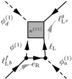
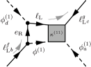
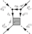
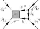
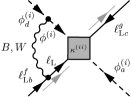
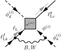
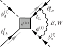
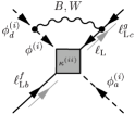
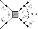
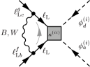
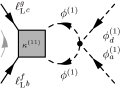
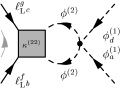
Figure 1: One-loop diagrams contributing to the vertex renormalization of $\kappa^{(ii)}$. The one-loop diagrams (a) – (d) that arise due to the Yukawa coupling $Y_{e}$ affect only the renormalization of $\kappa^{(11)}$. The one-loop gauge diagrams (e) – (j) are the same as in the SM. $B$ and $W\in\{W^{1},W^{2},W^{3}\}$ are the gauge bosons of $\text{SU}(1)_{\mathrm{Y}}$ and $\text{SU}(2)_{\mathrm{L}}$. Diagrams (k) – (n) come from the Higgs interaction Lagrangian. While the diagrams (k) and (l) have a counterpart in the SM, the diagrams (m) and (n) appear only in the 2HDM’s and lead to a mixing between the operators $\mathscr{L}_{\kappa}^{(11)}$ and $\mathscr{L}_{\kappa}^{(22)}$. The gray arrow indicates the fermion flow as defined in [6].

The relevant Feynman diagrams are shown in figure 1. Using the technique described in [2], the $\beta$-functions $\beta_{\kappa^{(ii)}}=\mu\frac{\mathrm{d}}{\mathrm{d}\mu}\kappa^{(ii)}$ with $\mu$ denoting the renormalization scale, can be obtained from the counterterms,

$$16\pi^{2}\beta_{\kappa^{(ii)}} = \left(\tfrac{1}{2}-2\delta_{i1}\right)\,\left[\kappa^{(ii)}(Y_{e}^{\dagger}Y_{e})+(Y_{e}^{\dagger}Y_{e})^{T}\kappa^{(ii)}\right]$$ (11)

$${}+\left[\delta_{i1}\,2\,\text{Tr}(Y_{e}^{\dagger}Y_{e})+z^{(i)}_{u}\,6\,\text{Tr}(Y_{u}^{\dagger}Y_{u})+z^{(i)}_{d}\,6\,\text{Tr}(Y_{d}^{\dagger}Y_{d})\right]\kappa^{(ii)}$$

$${}+\lambda_{i}\kappa^{(ii)}+\delta_{i1}\lambda_{5}^{*}\kappa^{(22)}+\delta_{i2}\lambda_{5}\kappa^{(11)}-3g_{2}^{2}\kappa^{(ii)}\;.$$

The terms proportional to $\lambda_{5}$ are responsible for the mixing of the effective operators mentioned before. Our result for $\beta_{\kappa^{(11)}}$ differs from the one in [7] by a factor of 3 because of the term $\tfrac{1}{2}-2\delta_{i1}$ in the first line. We had earlier found [2] an analogous discrepancy in $\beta_{\kappa}$ for the SM, which has recently been confirmed [8].

Note that in 2HDM’s running effects are in general larger than in the SM due to the fact that the Yukawa couplings are enhanced, e.g. $(Y_{e})_{\mathrm{2HDM}}=(Y_{e})_{\mathrm{SM}}/\cos\beta$, where $\tan\beta=v^{(1)}/v^{(2)}$ with $v^{(i)}$ being the vacuum expectation value of the Higgs field $\phi^{(i)}$.

3 The Effective Neutrino Mass Operator in the MSSM

In the MSSM, the effective dimension 5 operator that gives Majorana masses to the SM neutrinos is contained in the $F$-term of the superpotential

$$\mathscr{W}_{\kappa}^{\mathrm{MSSM}}=-\frac{1}{4}{\kappa}_{gf}\,\boldsymbol{L}^{g}_{c}\varepsilon^{cd}\boldsymbol{H}^{(2)}_{d}\,\,\boldsymbol{L}_{b}^{f}\varepsilon^{ba}\boldsymbol{H}^{(2)}_{a}+\text{h.c.}\;.$$ (12)

$\boldsymbol{L}$ and $\boldsymbol{H}^{(2)}$ are the chiral superfields that contain the SU(2)_L doublets, the Higgs doublet with weak hypercharge $+\tfrac{1}{2}$ and the corresponding superpartners. The part of the superpotential describing the Yukawa interactions is given by

$$\mathscr{W}_{\mathrm{Yuk}}^{\mathrm{MSSM}} = (Y_{e})_{gf}\boldsymbol{E}^{\mathrm{C}g}\boldsymbol{H}^{(1)}_{a}\varepsilon^{ab}\boldsymbol{L}^{f}_{b}$$ (13)

$${}+(Y_{d})_{gf}\boldsymbol{D}^{\mathrm{C}g}\boldsymbol{H}^{(1)}_{a}\varepsilon^{ab}\boldsymbol{Q}^{f}_{b}+(Y_{u})_{gf}\boldsymbol{U}^{\mathrm{C}g}\boldsymbol{H}^{(2)}_{a}(\varepsilon^{T})^{ab}\boldsymbol{Q}_{b}^{f}\;.$$

The superfields $\boldsymbol{E}^{\mathrm{C}}$, $\boldsymbol{D}^{\mathrm{C}}$ and $\boldsymbol{U}^{\mathrm{C}}$ contain the $\mathrm{SU}(2)_{\mathrm{L}}$-singlet charged leptons, down-type quarks and up-type quarks, respectively, and $\boldsymbol{Q}$ contains the SU(2)_L quark doublets. The Higgs superfield $\boldsymbol{H}^{(1)}$ has weak hypercharge $-\tfrac{1}{2}$. Calculating the RGE in the MSSM yields

$$16\pi^{2}{\beta}_{\kappa}^{\mathrm{MSSM}}=(Y_{e}^{\dagger}Y_{e})^{T}{\kappa}+{\kappa}(Y_{e}^{\dagger}Y_{e})+6\,\text{Tr}(Y_{u}^{\dagger}Y_{u})\,{\kappa}-2g_{1}^{2}{\kappa}-6g_{2}^{2}{\kappa}\;,$$ (14)

confirming the existing MSSM result [9, 7].

4 Conclusion

A recent check of the SM $\beta$-function [8] showed that previously published results were not quite correct. Therefore, in this letter we have derived the RGE’s for the effective dimension 5 operators which yield a Majorana mass for neutrinos after the electroweak symmetry breaking in four types of 2HDM’s and in the MSSM. For the MSSM, we confirmed the earlier result [9, 7]. However, when we applied our general result (11) to the 2HDM discussed in [7], we found that the non-diagonal part of one of the $\beta$-functions, relevant for the evolution of the mixing angles, is enhanced by a factor of 3.

References

[1]
For an introduction see for example:
E. K. Akhmedov, Neutrino physics, (2000),
hep-ph/0001264.
[2]
S. Antusch, M. Drees, J. Kersten, M. Lindner, M. Ratz,
Neutrino mass operator renormalization revisited, Phys. Lett.
B519 (2001), 238–242, (hep-ph/0108005).
[3]
S. Weinberg,
Gauge theory of CP violation,
Phys. Rev. Lett. 37 (1976), 657.
[4]
S. L. Glashow, S. Weinberg, Natural conservation laws for
neutral currents, Phys. Rev. D15 (1977), 1958.
[5]
E. A. Paschos, Diagonal neutral currents, Phys. Rev. D15
(1977), 1966.
[6]
A. Denner, H. Eck, O. Hahn, J. Küblbeck, Feynman rules for fermion
number violating interactions, Nucl. Phys. B387 (1992), 467–484.
[7]
K. S. Babu, C. N. Leung, J. Pantaleone, Renormalization of the
neutrino mass operator, Phys. Lett. B319 (1993), 191–198,
(hep-ph/9309223).
[8]
P. H. Chankowski, P. Wasowicz, Low energy threshold corrections
to neutrino masses and mixing angles, (2001), (hep-ph/0110237).
[9]
P. H. Chankowski, Z. Pluciennik, Renormalization group
equations for seesaw neutrino masses, Phys. Lett. B316 (1993),
312–317, (hep-ph/9306333).