Numerical modelling of Bose-Einstein correlations

Abstract

We propose extension of the algorithm for numerical modelling of Bose-Einstein correlations (BEC), which was presented some time ago in the literature. It is formulated on quantum statistical level for a single event and uses the fact that identical particles subjected to Bose statistics do bunch themselves, in a maximal possible way, in the same cells in phase-space. The bunching effect is in our case obtained in novel way allowing for broad applications and fast numerical calculations. First comparison with $e^{+}e^{-}$ annihilations data performed by using simple cascade hadronization model is very encouraging.

PACS numbers: 25.75.Gz 12.40.Ee 03.65.-w 05.30.Jp
Keywords: Bose-Einstein correlations; Statistical models; Fluctuations

Bose-Einstein correlations (BEC) between identical bosons are since long time of special interest because of their ability to provide space-time information about multiparticle production processes [1]. This is particulary true in searches for a proper dynamical evolution of heavy ion collisions (QGP) [2]. However, such processes, because of their complexity, must be modelled by means of Monte Carlo event generators [3], probabilistic structure of which prevents a priori the genuine BEC (which are of purely quantum statistical origin). One can only attempt to model BEC in some way aiming to reproduce the two-particle correlation function measured experimentally and defined, for example, as ratio of the two-particle distributions to the product of single-particle distributions:

$$C_{2}(Q=|p_{i}-p_{j}|)\,=\,\frac{N_{2}(p_{i},p_{j})}{N_{1}(p_{i})\,N_{1}(p_{j})}.$$ (1)

This is done either by changing the original output of these generators by artificially bunching in phase-space (in a suitable way) the finally produced identical particles [4, 5] or by constructing generator, which allows to account from the very beginning for the bosonic character of produced secondaries [6]. In former case the simplest approach is to shift (in each event) momenta of adjacent like-charged particles in such a way as to get desired $C_{2}(Q)$ [4] and to correct afterwards for the energy-momentum imbalance introduced this way. Much more physical is the method developed in [5], which screens all events against the possible amount of bunching they are already showning and counts them as many times as necessary to get desirable $C_{2}(Q)$. The original energy-momentum balance remains in this case intact whereas the original single particle distributions are changed (this fact can be corrected by running again generator with suitably modified input parameters). The size parameters occuring in weights bear no direct resemblance to the size parameter $R$ obtained by directly fitting data on $C_{2}(Q)$ in eq.(1) by, for example, simple gaussian form: $C_{2}(Q)=c\left[1+\lambda\exp\left(-R^{2}Q^{2}\right)\right]$ (where $c$ is normalization constant, $\lambda$ the so called chaoticity and $R$ the size parameter). They represent instead the corresponding correlation lengths between the like particles [1].

The approach proposed in [6] represents different philosophy of getting desired bunching. Here one uses specific generator, which groups (already on a single event level) bosonic particles of the same charge in a given cell in phase space according to Bose-Einstein distribution,

$$P(E_{i})\sim\exp\left[\frac{n_{i}\left(\mu-E_{i}\right)}{T}\right].$$ (2)

Here $n_{i}$ is their multiplicity and $E_{i}$ energy, the energy-momentum and charge conservations are strictly imposed by means of the information theory concept of maximazing suitable information entropy. The parameters $T$ and $\mu$ are therefore two lagrange multipliers with values fixed by the energy-momentum and charge conservation laws, respectively. Such distribution is typical example of nonstatistical fluctuations present in the hadronizing source. With only one additional parameter $\delta y$, which denotes the size of the elementary emitting cell in phase-space (in [6] it means in rapidity), one gets at the same time both the correct BEC pattern (i.e., correlations) and fluctuations (as characterized by intermittency) [6]. This is very strong advantage of this model, which is so far the only example of hadronization model, in which Bose-Einstein statistics is not only included from the very beginning on a single event level, but it is also properly used in getting final secondaries. In all other approaches at least one of the above elements is missing. The shortcoming of method [6] are numerical difficulties to keep the energy-momentum conservation as exact as possible and limitation to the specific event generator only.

In the present work we propose generalization of this approach making it applicable to other generators. Namely, following the same reasoning as in [6, 9], we propose different method of introducing desired bunching. In [6] the generator itself provided particles satisfying Bose statistics (in the sense mentioned above). In the general case one has to find the possible bosonic configurations of secondaries existing already among the produced particles. The point is that nonstatistical fluctuations present in each event generator result in a nonuniform (bunched) distributions of particles produced in a given event in momentum space. They resemble Bose distribution provided by the statistical event generator of [6], the only difference being that particles in such bunches usually have different charges allocated to them by event generator, whereas in [6] particles were of the same charge. We propose therefore to maximally equalize charges of particles in such bunches (to the extent limited only by the overall charge conservation) superseeding the initial charge allocation provided by event generator (keeping only intact the total number of particles of each charge it gives). This is supposed to be done in each single event. Both the original energy-momentum pattern provided by event generator and all inclusive single particle distributions are left intact.

It is instructive to look at this problem from yet another point of view. Namely, it can be perceived as an attempt (cf. [11]) to model correlations of fluctuations present in the system, as given by:

$$\langle n_{1}n_{2}\rangle = \langle n_{1}\rangle\langle n_{2}\rangle+\langle\left(n_{1}-\langle n_{1}\rangle\right)\left(n_{2}-\langle n_{2}\rangle\right)\rangle$$ (3)

$$= \langle n_{1}\rangle\langle n_{2}\rangle+\rho\sigma(n_{1})\sigma(n_{2}).$$

Here $\sigma(n)$ is dispersion of the multiplicity distribution $P(n)$ and $\rho$ is the correlation coefficient depending on the type of particles produced: $\rho=+1,-1,0$ for bosons, fermions and Boltzmann statistics, respectively. The proposed algorithm should provide us with $C_{2}(Q)$, which is in fact a measure of correlation of fluctuations because

$$C_{2}(Q=|p_{i}-p_{j}|)=\frac{\langle n_{i}\left(p_{i}\right)n_{j}\left(p_{j}\right)\rangle}{\langle n_{i}\left(p_{i}\right)\rangle\langle n_{j}\left(p_{j}\right)\rangle}=1+\rho\frac{\sigma\left(n_{i}\right)}{\langle n_{i}\left(p_{i}\right)\rangle}\frac{\sigma\left(n_{j}\right)}{\langle n_{j}\left(p_{j}\right)\rangle}.$$ (4)

To get $\rho>0$ (in which we are interested here) it is enough to select one of the produced particles, allocate to it some charge, and then allocate (in some prescribe way) the same charge to as many particles located near it in the phase space as possible (limited only by the charge conservation constraint). In this way one forms a cell in phase-space, which is occupied by particles of the same charge only. This process should then be repeated until all particles are used and it should be done in such way as to get geometrical (Bose-Einstein) distribution of particles in a given cell. We stress again that this procedure does not alter neither the original energy-momentum distributions nor the spatio-temporal pattern of particles provided by event generator. It only changes the charge flow pattern it provides retaining, however, both the initial charge of the system and its total multiplicity distribution. Therefore this method works only when we can resign from controlling the charge flow during hadronization process.

The procedure of formation of such cells is controlled by a parameter $P$ being the probability that given neighbor of the initially selected particle should be counted as another member of the newly created emmiting cell in phase space. Notice that any selection procedure leading to a geometrical particle distribution in cells (in which case $\sigma=<n>$) results in maximization of the second term in the eq. (4). In particular it can be realized by the following algorithm of allocation of charges (the $n_{l}=n_{l}^{(+)}+n_{l}^{(-)}+n_{l}^{(0)}$ is the number of particles of different charges provided by our event generator in the $l^{th}$ event, $\{p_{j}\}$ and $\{x_{i}\}$ are, respectively, their energy-momenta and spatio-temporal positions, which we keep intact):

• The SIGN is chosen randomly from: ”+”, ”-”or ”0” pool, with probabilities given by $p^{(+)}_{l}=n_{l}^{(+)}/n_{l}$, $p^{(-)}_{l}=n_{l}^{(-)}/n_{l}$ and $p^{(0)}_{l}=n_{l}^{(0)}/n_{l}$. It is attached to particle $(i)$ chosen randomly from the particles produced in this event and not yet reassigned new charges.

• Distances in momenta, $\delta_{ij}(p)=\left|p_{i}-p_{j}\right|$, between the chosen particle $(i)$ and all other particles $(j)$ still without signs are calculated and arranged in ascending order with $j=1$ denoting the nearest neighbor of particle $(i)$. To each $\delta_{ij}(p)$ one assignes some probability $P(i,j)\in(0,1)$.

• A random number $r\in(0,1)$ is selected from a uniform distribution. If $n^{SIGN}_{l}>0$, i.e., if there are still particles of given SIGN with not reassigned charges, one checks the particles $(j)$ in ascending order of $j$ and if $r<P(i,j)$ then charge SIGN is assigned also to the particle $(j)$, the original multiplicity of particles with this SIGN is reduced by one, $n^{SIGN}_{l}=n^{SIGN}_{l}-1$, and the next particle is selected: $(j)\Rightarrow(j+1)$. However, if $r>P(i,j)$ or $n^{SIGN}_{l}=0$ then one returns to point $(1)$ with the updated values of $p_{l}^{(+)},~{}p_{l}^{(-)}$ and $p_{l}^{(0)}$. Procedure finishes when $n_{l}^{(+)}=n_{l}^{(-)}=n_{l}^{(0)}=0$, in which case one proceeds to the next event.

As can be easily checked, this algorithm results in geometrical (Bose-Einstein) distribution of particles in the phase-space cells formed by our procedure (with mean multiplicity $P/(1-P)$ for constant $P(ij)=P$ case) accounting therefore for their bosonic character (i.e., for Bose-Einstein statistics they should obey).

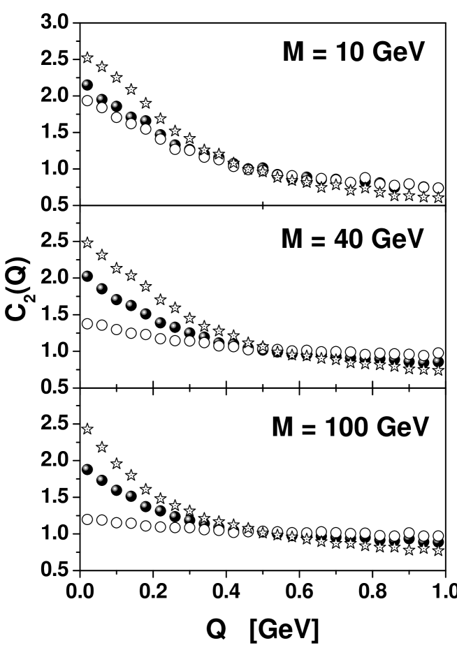
Figure 1: Examples of BEC patterns obtained for $M=10$, $40$ and $100$ GeV for constant weights $P=0.75$ (stars) and $P=0.5$ (full symbols) and for the weight given by eq.(5) (open symbols).

We shall illustrate now action of our algorithm on simple cascade model of hadronization (CAS) (in its one-dimensional versions and assuming, for simplicity, that only direct pions are produced)[12]. In CAS the initial mass $M$ hadronizes by series of well defined (albeit random) branchings ($M\rightarrow M_{1}+M_{2}$) and is endowed with a simple spatio-temporal pattern. It shows no traces of Bose-Einstein statistics whatsoever. However, as can be seen in Fig. 1, when endowed with charge selection provided by our algorithm, a clear BEC pattern emerges in $C_{2}(Q)$. Two kind of choices of probabilities are shown in Fig. 1. First is constant $P=0.75$ and $P=0.5$. It leads to a pure geometrical distribution of number of particles allocated to a given cell and corresponds to situation already encountered in [6]. Its actual value is so far a free parameter replacing, in a sense, the parameter $\delta y$ in [6]. However, whereas in [6] the size of emitting cells was fixed, in our case it is fluctuating. The other is what we call the ”minimal” weight constructed from the output information provided by CAS event generator:

$$P(ij)=\exp\left[-\frac{1}{2}\delta^{2}_{ij}(x)\cdot\delta^{2}_{ij}(p)\right]$$ (5)

where $\delta_{ij}(x)=|x_{i}-x_{j}|$ and $\delta_{ij}(p)=|p_{i}-p_{j}|$. In this way one connects $P$ with details of hadronization process by introducing to it a kind of overlap between particles as a measure of probability of their bunching in a given emitting cell.

As we have checked out the BEC effect occuring here depends only on the (mean) number of particles of the same charge in phase-space cell and on the (mean) numbers of such cells. This depends on $P$, the bigger $P$ the more particles and bigger $C_{2}(Q=0)$; smaller $P$ leads to the increasing number of cells, which, in turn, results in decreasing $C_{2}(Q=0)$, as already noticed in [9]. For small energies the number of cells decreases in natural way while their occupation remains the same (because $P$ is the same), therefore the corresponding $C_{2}(0)$ is bigger, as seen in Fig. 1. The fact that there is tendency to have $C_{2}(0)>2$ for larger $P$ means that one has in this case more cells with more than $2$ particles allocated to them, i.e., it is caused by the influence of higher order BEC. Therefore the ”sizes” $R$ obtained from the exponential fits to results in Fig. 1 (like $C_{2}(Q)\sim 1+\lambda\cdot\exp(-Q\cdot R)$ where $\lambda$ being usually called chaoticity parameter [1]) correspond to the sizes of the respective elementary cells rather than to sizes of the whole hadronizing sources itself. For $P=0.5$ the ”size” $R$ varies weakly between $0.66$ to $0.87$ fm from $M=10$ to $100$ GeV whereas for the ”minimal” weight (5) it varies from $0.64$ to $0.44$ fm .

So far we were considering only single sources. Suppose now that source of mass $M$ consists of a number ($n_{l}=2^{k}$) of subsources hadronizing independently. It turns out that the resulting $C_{2}$’s are very sensitive to whether in this case one applies our algorithm of assigning charges to all particles from subsources taken together (”Split” type of sources) or to each of the subsource independently (”Indep” type of sources), cf. Fig. 2. Whereas the later case results in the similar ”sizes” $R$ (defined as before) with $C_{2}(Q=0)-1=\lambda$ falling dramatically with increasing $k$ (roughly like $1/2^{k}$, i.e., inversely with the number of subsources, $n_{l}$, as expected fom [9]), the former leads to roughly the same $C_{2}(Q=0)$ but the ”size” $R$ is now increasing substantially being equal to, respectively, $0.87$ fm, $1.29$ fm, $1.99$ fm and $3.35$ fm for $P=0.5$ and $0.57$ fm, $3.26$ fm, $4.01$ and $5.59$ fm for the ”minimal” weight (5). Fig. 3 contains example of our ”best fit” to the $e^{+}e^{-}$ annihilation data on BEC by DELPHI Collaboration [13] for $M=91.3$ GeV (which can be obtained only for two or three subsources, as shown there).

To summarize: we propose a new and simple method of numerical modelling of BEC. It is based on reassigning charges of produced particles in such a way as to make them look like particles satisfying Bose statistics, conserves the energy-momenta and does not alter the spatio-temporal pattern of events or any single particle inclusive distribution (but it can change the distributions of, separately, charged and neutral particles leaving, however, the total distribution intact). It is intended to be a kind of suitable extension of the algorithm presented in [6], such that can be applied to essential any event generator in which such reassignment of charges is possible. It amounts to the changes in physical picture of the original generator. The example of CAS is very illustrative in this respect. In it, at each branching vertex one has, in addition to the energy-momentum conservation, imposed strict charge conservation and one assumes that only $(0)\rightarrow(+-)$, $(+)\rightarrow(+0)$ and $(-)\rightarrow(-0)$ transitions are possible. It means that there are no multicharged vertices (i.e., vertices with multiple charges of the same sign) in the model. However, after applying to the finally produced particles our charge reassignment algorithm one finds, when working the branching tree ”backwards”, that precisely such vertices occur now (with charges ”(++)”, or ”(- -)”, for example). The total charge is, however, still conserved as are the charges in decaying vertices (i.e., no spurious charge is being produced because of our algorithm). It is plausible therefore that to get BEC in an event generators it is enough to allow for cumulation of charges of the same sign at some points of hadronization procedure modelled by this generator. This would lead, however, to extremely difficult numerical problem with ending such algorithms without producing spurious multicharged particles not observed in nature.

We find that value of $C_{2}(Q=0)$ (defining chaoticity parameter $\lambda$) depends inversely on the number of elementary cells, in the way already discussed in [9], and that ”radius” $R$ extracted from the exponential fits is practically independent on the size of the source, provided it is a single one. In the case when it is composed of a number of elementary sources, $R$ increases with their number, unless they are treated independently by our algorithm. It is because one has in this case a higher density of particles. This results in smaller average $Q$, and this in turn leads to bigger $R$. On the contrary, for the independently treated sources the density of particles subjected to our algorithm does not change, hence the average $Q$ and $R$ remain essentially the same. However, because in this case the influence of pairs of particles from different subsources increases, the effective $\lambda=C_{2}(0)-1$ now decreases substantially (as was already observed in [9]). It should be mentioned at this point that our ”Indep” type sources can probably be used as a possible explanation of the so called inter-$W$ BEC problem, i.e., the fact that essentially no BEC is being observed between pions originating from a different $W$ in fully $W^{+}W^{-}$ final states [16]. It can be understood by assuming that produced $W$’s should be treated as ”Indep” type sources for which $\lambda$ falls dramatically. Finally, we would like to stress that our algorithm leads to strong intermittency showing up after its application. It means that with such algorithm (which is very efficient and fast for all multiplicities) we can already attempt to fit experimental data by applying it to some more sophisticated fragmentation schemes than that provided by CAS. This will be done elsewhere.

Acknowledgements:
The partial support of Polish Committee for Scientific Research (grants 2P03B 011 18, 5P03B 091 21 and 621/ E-78/ SPUB/ CERN/P-03/DZ4/99) is acknowledged. The fruitful and stimulating discussions with B.Andersson, K.Fiałkowski, T.Csörgő W.Kittel and S.Todorova-Nova, are gratefully acknowledged.

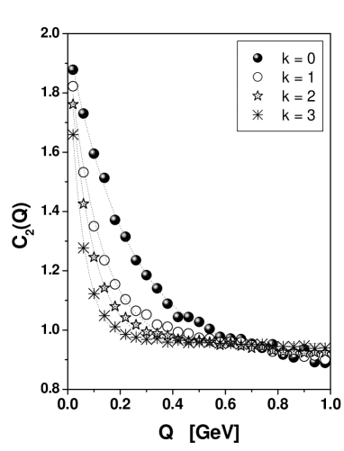
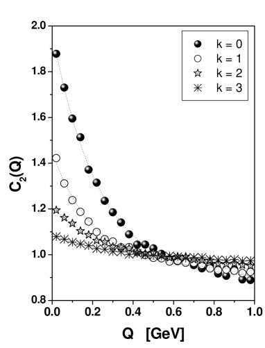
Figure 2: Examples of BEC for different number of subsources ($n_{l}=2^{k}$, $k=1,2,3$ existing in the source $M=100$ GeV. Left panel is for the ”Split” and right panel for the ”Indep” types of sources, as discussed in text.

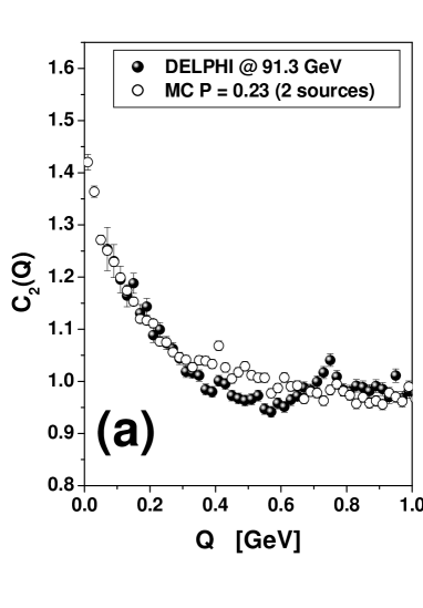
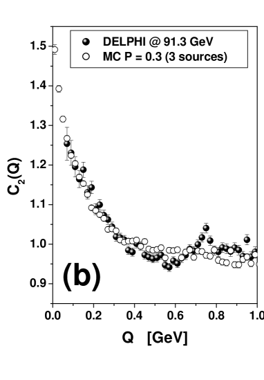
Figure 3: The examples of the ”best fits” to the $e^{+}e^{-}$ annihilation data on BEC by DELPHI [13] using $2$ $(a)$ or $3$ $(b)$ subsources with $P=0.23$ and $P=0.3$, respectively.

References

- [1] R.M.Weiner, Phys. Rep. 327, 249 (2000); U.A.Wiedemann and U.Heinz, Phys. Rep. 319, 145 (1999); T.Csörgő, in Particle Production Spanning MeV and TeV Energies, eds. W.Kittel et al., NATO Science Series C, Vol. 554, Kluwer Acad. Pub. (2000), p. 203 (see also: hep-ph/0001233).
- [2] Cf. proceedings of any Quark Matter conference and references therein, for example QM99, eds. L.Riccati et al., Nucl. Phys. A661 (1999).
- [3] K.J.Escola, On predictions of the first results from RHIC, hep-ph/0104058, to be published in Proc. of QM2001, Nucl. Phys. A (2001).
- [4] L.Lönnblad and T.Sjöstrand, Eur. Phys. J. C2, 165 (1998).
- [5] A.Białas and A.Krzywicki, Phys. Lett. B354, 134 (1995); K.Fiałkowski and R.Wit, Eur. Phys. J. C2, 691 (1998); K.Fiałkowski, R.Wit and J.Wosiek, Phys. Rev. D58, 094013 (1998); T.Wibig, Phys. Rev. D53, 3586 (1996).
- [6] T.Osada, M.Maruyama and F.Takagi, Phys. Rev. D59, 014024 (1999).
- [7] B.Andersson, Acta Phys. Polon. B29 (1998) 1885 and references therein.
- [8] J.P.Sullivan et al., Phys. Rev. Lett. 70, 3000 (1993); K.Geiger, J.Ellis, U.Heinz and U.A.Wiedemann, Phys. Rev. D61, 054002 (2000).
- [9] M.Biyajima, N.Suzuki, G.Wilk and Z.Włodarczyk, Phys. Lett. B386, 297 (1996).
- [10] H.Merlitz and D.Pelte, Z. Phys. A351, 187 (1995) and Z. Phys. A357, 175 (1997); U.A.Wiedemann et al., Phys. Rev. C56, R614 (1997); T.Csörgő and J.Zimányi, Phys. Rev. Lett. 80, 916 (1998) and Heavy Ion Phys. 9, 241 (1999).
- [11] K.Fiałkowski, in Proc. of the XXX ISMD, Tihany, Hungary, 9-13 October 2000, Eds. T.Csörgő et al., World Scientific 2001, p. 357; M.Stephanov, Thermal fluctuations in the interacting pion gas, hep-ph/0110077.
- [12] O.V.Utyuzh, G.Wilk and Z.Włodarczyk, Phys. Rev. D61, 034007 (2000) and Czech J. Phys. 50/S2, 132 (2000) (hep-ph/9910355).
- [13] P.Abreu et al. (DELPHI Collab.), Phys. Lett. B286 (1992) 201.
- [14] B.Buschbeck and H.C.Eggers, Nucl. Phys. B (Proc. Suppl.) 92 (2001) 235.
- [15] Cf. [7] and private communication by B.Andersson.
- [16] Cf. Š.Todorova-Nová, in Proc. of the XXX ISMD, Tihany, Hungary, 9-13 October 2000, Eds. T.Csörgő et al., World Scientific 2001, p. 343 (hep-exp/0202057) and references therein.