Analytic continuation and perturbative expansions in QCD
Irinel Caprini

National Institute of Physics and Nuclear Engineering, POB MG 6,

Bucharest, R-76900 Romania, and

The Abdus Salam International Centre for Theoretical Physics, Trieste, Italy

Jan Fischer

Institute of Physics, Academy of Sciences of the Czech Republic,

CZ-182 21 Prague 8, Czech Republic

Starting from the divergence pattern of perturbative quantum chromodynamics, we propose a novel, non-power series replacing the standard expansion in powers of the renormalized coupling constant $a$. The coefficients of the new expansion are calculable at each finite order from the Feynman diagrams, while the expansion functions, denoted as $W_{n}(a)$, are defined by analytic continuation in the Borel complex plane. The infrared ambiguity of perturbation theory is manifest in the prescription dependence of the $W_{n}(a)$. We prove that the functions $W_{n}(a)$ have branch point and essential singularities at the origin $a=0$ of the complex $a$-plane and their perturbative expansions in powers of $a$ are divergent, while the expansion of the correlators in terms of the $W_{n}(a)$ set is convergent under quite loose conditions.

1 Introduction

The standard QCD perturbative expansion in powers of the renormalization group improved coupling is plagued by several deficiencies. The series is divergent and even Borel non-summable, having a zero convergence radius [1]-[2] and coefficients exhibiting asymptotically factorial growth and nonalternating signs [3]-[8]. The truncated, fixed order perturbative expansion is afflicted with the problem of renormalization scheme dependence and violates explicitly, due to the Landau singularities, the rigorous momentum plane analyticity imposed by general principles for confined theories [9]. Several resummations or reformulations of the perturbative expansion have been considered recently, trying to cure or reduce these deficiencies. Modified expansions which eliminate the unphysical singularities in the momentum plane were proposed in [10], [11]. Reformulations of the perturbation theory attempting to reduce the renormalization scheme dependence of the truncated series were also proposed by several authors, using concepts like minimal sensitivity [12], effective charge [13], [14] or Padé approximants in the complex plane of the coupling constant [15]-[17].

Other attempts to go beyond the conventional perturbative expansion are motivated by the large order behaviour of perturbation theory [18]-[22]. The perturbation theory is intrinsically ambiguous, due to the infrared regions of the Feynman diagrams. According to current views [21], the perturbative ambiguity will be compensated in the complete theory by the nonperturbative contributions. But the estimate of this intrinsic ambiguity is made difficult by the fact that the series is divergent, and the higher terms dramatically spoil the accuracy of the result above a certain order. If one succeeded to replace the usual perturbative expansion by a convergent series (each new term improving the accuracy of the approximation instead of spoiling it), the intrinsic ambiguity of perturbation theory would be better defined. In the present work we address this problem and propose a new, non-power perturbative expansion in QCD, using the principle of analytic continuation in the Borel complex plane.

Although the perturbative series in QCD is not Borel summable, since the conditions for Borel summability [23], [24] are not satisfied, the notion of Borel transform of the QCD correlators is nevertheless useful, as its singularities in the Borel plane contain much physical information. The infrared (IR) and ultraviolet (UV) renormalons and the instantons define a generic doubly-cut Borel plane, which provides an intuitive measure of the ambiguities of the perturbation theory.

The conformal mapping of the Borel plane was suggested in [25] as a technique to reduce or eliminate the ambiguities (power corrections) due to the large momenta in the Feynman integrals. Such conformal mappings, which move the UV renormalons further from the origin [26], [27] exploit however only in part the known singularity structure in the Borel plane. An optimal mapping, which performs the analytic continuation in the whole doubly-cut Borel plane, was considered in our previous papers [28], [29] (similar mappings were applied later in [30], [31]). By means of this technique, we defined in [29] a non-power perturbative expansion in QCD in terms of a new set of functions that fully exploit the location of the singularities in the Borel plane.

In the present paper we study the properties of these expansion functions, denoted below as $W_{n}(a)$, and the role of the modified expansion for a better understanding of the ambiguities inherent in perturbative QCD. The results are impressive: in contrast to the perturbative powers $a^{n}$, the new functions $W_{n}(a)$ provide a convergent expansion of the correlator in a large domain of the coupling constant complex plane, and share in addition certain important properties with the expanded correlator itself.

The paper is organized as follows: in section 2 we recall the basic facts known about the singularities of the QCD correlation functions in the Borel plane and discuss the method of optimal conformal mapping. We use for illustration the Adler function in massless QCD, but the generalization to other cases is straightforward. In section 3 we define the functions $W_{n}(a)$ and the modified perturbative expansion replacing the standard series in powers of the coupling constant. We investigate the analytic properties of the expansion functions in the complex $a$-plane, their asymptotic expansions for small $a$, and the convergence conditions for the new expansion. In the concluding section 4, we point out the specific merits of the modified expansion for defining the intrinsic ambiguity of perturbation theory.

2 Conformal mapping of the Borel plane

2.1 Singularities in the Borel plane

We consider the Adler function in massless QCD

$$D=-4\pi^{2}s\left(\frac{{\rm d}}{{\rm d}s}\right)\Pi(s)\,,$$ (1)

where $\Pi(s)$ is the amplitude of the electromagnetic current–current correlation function

$$\Pi^{\mu\nu}(p)=i\int{\rm d}^{4}x{\rm e}^{-ipx}\langle 0|\,{\rm T}(j^{\mu}(x)j^{\nu}(0))\,|0\rangle$$

$$=(g^{\mu\nu}p^{2}-p^{\mu}p^{\nu})\Pi(s)\,,\quad s=p^{2}\,.$$ (2)

In perturbative QCD, the function $D$ can be formally expanded in powers of the renormalized coupling constant $\alpha_{s}(\mu^{2})$

$$D=\sum_{n=0}^{\infty}D_{n}\left({\alpha_{s}(\mu^{2})\over\pi}\right)^{n}\,,$$ (3)

where the coefficients $D_{n}$ depend on the external momentum squared $s$, and are renormalization scheme and scale dependent. Certain classes of Feynman diagrams suggest that they are factorially increasing with $n$, therefore the series (3) is divergent, and has to be given a precise meaning.

Among various summation techniques of power series [23], [24], the Borel method received much interest in recent years, although the mathematical conditions required for its use are not satisfied in QCD [1], [2]. As mentioned in the Introduction, even if the Borel summation method is not applicable it is useful to examine and exploit the singularity structure of the Borel transform, as it contains important physical information. In the present paper we use the Borel transform to define an improved perturbative expansion, using in addition the principle of analytic continuation.

The Borel transform of the Adler function is defined by the power series

$$B(u,s)=\sum\limits_{n=0}^{\infty}b_{n}u^{n}\,,$$ (4)

with $b_{n}$ related to the original perturbative coefficients appearing in (3) by

$$b_{n}={D_{n}\over\beta_{0}^{n}n!}\,,$$ (5)

where $\beta_{0}$ is the first coefficient of the $\beta$ function. Then the Adler function given by the series (3) can be formally expressed as the Laplace transform

$$D(s,a)={1\over a}\,\int\limits_{0}^{\infty}\!{\rm e}^{-u/a}\,B(u,s)\,{\rm d}u\,,$$ (6)

where $a=\beta_{0}\alpha_{s}(\mu^{2})/\pi$.

The Borel transform $B(u,s)$ is scheme and scale dependent. As discussed in [21], in the large $N_{f}$ limit the momentum dependence can be factorized as

$$B(u,s)=\left({-s{\rm e}^{C}\over\mu^{2}}\right)^{-u}B_{0}(u)\,,$$ (7)

where $C$ is a scheme-dependent constant. The power factor in (7) combines with the exponential in (6) in a renormalization scheme and scale independent quantity, the remaining factor $B_{0}(u)$ also being scheme and scale independent. The validity of a similar factorization beyond the large $N_{f}$ limit is an open question [21]. However, it is generally assumed that the position of the singularities of the function $B(u,s)$ in the Borel $u$ plane is independent of renormalization scheme and scale, and also of the external momenta (as discussed in [21], this is expected to be the case at least in the so-called ”regular schemes”).

The method developed in the present paper is based on the analytic continuation in the Borel plane, requiring therefore the knowledge of the singularity structure in this plane. We shall assume that the location of the singularities of the Borel transform is known and is independent of the renormalization scheme. For the Adler function, the coefficients $D_{n}$ are assumed to have the specific large order increase

$$D_{n}\sim\sum\limits_{k}C_{k}\,n!\,n^{\delta_{k}}\left({\pi\beta_{0}\over k}\right)^{n}\,,$$ (8)

where the $k$ in the sum are integers, with $C_{k}$ and $n_{k}$ depending in general on $s$ and $\mu^{2}$. This behaviour leads to branch point singularities for the function $B$ in the $u$-plane, along the negative axis (the ultraviolet renormalons) and the positive axis (the infrared renormalons). Specifically, the branch cuts are situated along the rays $u\leq-1$ and $u\geq 2$ (see Fig. 1), and the nature of the first branch points was established in [25] and in [32]. The additional singularities due to the instanton–anti-instanton pairs [33] are situated at larger positive values of $u$, and will not influence the method discussed in this paper.

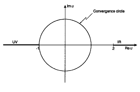
Figure 1: The Borel plane for the Adler function.

2.2 Optimal conformal mapping

The singularities of the Borel transform produce the perturbative ambiguities of the QCD correlators. For the Adler function, the Taylor expansion (4) of the Borel transform converges on the disk $|u|<1$ that reaches the nearest singularity, which is the first UV renormalon. The corresponding power correction ambiguity is however related to large momenta in the Feynman diagrams, and can be minimized or eliminated in QCD within perturbation theory. As suggested in Ref. [25], this can be achieved by an analytic continuation outside the convergence circle, by means of a conformal mapping. This method was investigated in [26], [27], using the mapping

$$v(u)=\frac{\sqrt{1+u}-1}{\sqrt{1+u}+1}\,,$$ (9)

and the corresponding expansion

$$B(u,s)=\sum\limits_{n=0}^{\infty}d_{n}v^{n}(u)\,,$$ (10)

instead of the power series (4). The mapping (9) transforms the UV cut $u\leq-1$ in the $u$-plane onto the unit circle $|v|=1$ in the $v$ plane, while the IR cut $u\geq 2$ remains inside the disk $|v|<1$ (see Fig. 2). As a consequence, the series (10) converges inside the small circle, which touches the image of the lowest IR renormalon in the $v$-plane. Thus, although the UV ambiguities (power corrections) are in principle eliminated by this method, the series (10) remains divergent along the positive semiaxis, the IR cut being outside the convergence circle.

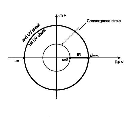
Figure 2: The $v$-complex plane. The UV cut is mapped upon the unit circle, while the IR cut is situated inside it. The convergence domain of the series (10) is limited by $u=2$, the lowest branch point of the IR cuts family.

The analytic continuation of the perturbative Borel transform into the whole holomorphy domain ${\cal D}$ can be performed by an optimal conformal mapping, $w(u)$, which maps the whole ${\cal D}$ onto the unit disk [34]. For the Adler function this mapping is [28]

$$w(u)=\frac{\sqrt{1+u}-\sqrt{1-u/2}}{\sqrt{1+u}+\sqrt{1-u/2}}\,.$$ (11)

The two branch points of $w(u)$, $u=-1$ and $u=2$, coincide with the lowest branch points of the Borel transform $B(u,s)$, while the corresponding two cuts, $u\leq-1$ and $u\geq 2$, cover the other branch points of $B$. As shown in Fig. 3, these two rays are mapped by (11) onto the boundary circle of the unit disk $|w|=1$ in the $w-$plane. The inverse of the mapping (11) is

$$u={8w\over 3w^{2}-2w+3}={8w\over 3(w-\zeta)(w-\zeta^{*})}\,,$$ (12)

where $\zeta=(\sqrt{2}+i)/(\sqrt{2}-i)$ and its complex conjugate $\zeta^{*}$ are the images of $u=\infty$ on the unit circle.

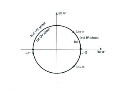
Figure 3: The $w$-complex plane. Both the UV cut and the IR cut are mapped upon the boundary unit circle. Inside it, there is no singularity. The convergence domain is the whole (cut) Borel plane.

As proposed in [28], we expand $B$ in powers of the variable $w$

$$B(u,s)=\sum_{n=0}^{\infty}c_{n}w^{n}(u),$$ (13)

where the coefficients $c_{n}$ can be obtained from the coefficients $b_{k}$, $k\leq n$, using Eqs. (4) and (11). By expanding $B(u,s)$ according to (13) one makes full use of its holomorphy domain, because the known part of it (i.e. the first Riemannian sheet) is mapped onto the convergence disk. The series (13) converges inside the whole disk $|w|<1$, i.e., in the whole cut $u$ plane, up to the cuts. A very important property, proved in [34], is that the expansion (13) has the fastest asymptotic (large-order) convergence rate, compared to any other expansion in powers of a variable that maps only a smaller part of the holomorphy domain onto the unit disk. We recall that the large-order convergence rate of a power series is equal to that of the geometrical series with the quotient $r/R$, $r$ being the distance of the point from the origin, and $R$ the convergence radius. The proof given in [34] consists in comparing the magnitudes of the ratio $r/R$ for a certain point in different complex planes, corresponding to different conformal mappings. When the whole analyticity domain ${\cal D}$ of the function is mapped on a disk, the value of $r/R$ is minimal [34].

3 Modified QCD perturbative expansion

3.1 Non-power expansion functions in QCD

The expansion (13) of the Borel transform suggests to expand the Adler function in the series [28, 29]

$$D(s,a)=\sum_{n=0}^{\infty}c_{n}W_{n}(a)\,,$$ (14)

where the functions $W_{n}(a)$ are defined as Laplace transforms of $w^{n}(u)$ :

$$W_{n}(a)={1\over a}\int\limits_{0}^{\infty}\,{\rm e}^{-u/a}\,w^{n}(u)\,{\rm d}u\,,\quad n=0,1,2,\ldots\,.$$ (15)

At each finite truncation order $N$, the expansion (14) is obtained by inserting the series (13) into the Laplace integral (6) and exchanging the order of summation and integration. This procedure is trivially allowed at any finite integer $N\geq 0$. For $N\to\infty$, however, the new expansion (14) represents a nontrivial step out of perturbation theory, replacing the perturbative powers $a^{n}$ by the functions $W_{n}(a)$. As proved in [29], the expansion (14) converges under certain rather general conditions (we discuss this point below in subsection 3.4). The convergence of the series (14) is our key argument in favor of the stepping out of the standard perturbation theory.

Our procedure is an obvious generalization of the conformal mapping method proposed in [36] for Borel summable functions. Formally, the expansion (14) is obtained from the standard perturbative expansion (3) by replacing the coefficients $b_{n}$, appearing in the Taylor series (4), by the coefficients $c_{n}$ of the improved expansion (13), and the perturbative functions $n!a^{n}$ (which multiply the coefficients $b_{n}$) by the new functions $W_{n}(a)$ defined by the integral (15). Actually, this integral is not well-defined since the branch-point $u=2$ is encountered along the integration range. This is a manifestation of the intrinsic ambiguity of the perturbation theory produced by the infrared renormalons. In defining the functions $W_{n}$, we shall use the same prescription as the one adopted in (6) for the correlator $D$ itself. We shall consider in particular the functions

$$W_{n}^{(\pm)}(a)={1\over a}\int\limits_{\cal C_{\pm}}\,{\rm e}^{-u/a}\,w^{n}(u)\,{\rm d}u\,,\quad n=0,1,2,\ldots\,,$$ (16)

where ${\cal C_{+}}$ (${\cal C_{-}}$) are lines parallel to the real positive axis, slightly above (below) it, and the principal value (PV) prescription

$$W_{n}^{(PV)}(a)={1\over 2}[W_{n}^{(+)}(a)+W_{n}^{(-)}(a)]\,.$$ (17)

In what follows we shall examine the expansion functions $W_{n}(a)$, showing that in many respects they resemble the expanded function $D(s,a)$ itself.

3.2 Analytic properties of $W_{n}(a)$ in the complex $a$-plane

The problem of the analytic properties of the QCD correlators in the coupling constant plane is very complex. ’t Hooft [1] and Khuri [2] showed that renormalization group invariance and the multiparticle branch-points on the timelike axis of the momentum plane $s=p^{2}$ imply a complicated accumulation of singularities near the point $a=0$. Since the proof uses a nonperturbative argument (multiparticle states generated by confinement in massless QCD), it is difficult to see this feature in perturbation theory, even in partial resummations that take into account infinite classes of Feynman diagrams.

In the present subsection we shall discuss the analytic properties of the expansion functions $W_{n}(a)$ defined by the integrals (16). Since the integrand is bounded, $|w^{n}(u)|<1$, the integrals converge for ${\rm Re}a>0$, i.e. $-\pi/2+\delta\leq\psi\leq\pi/2-\delta$, for $\delta>0$ arbitrarily small, where $\psi$ is the phase of $a$ ($a=|a|{\rm e}^{i\psi}$). Let us consider the functions $W_{n}^{(+)}(a)$ and take first $a$ complex in the first quadrant, i.e. $0<\psi<\pi/2$. Then we can rotate the integration contour ${\cal C}_{+}$ in (16) towards the upper quadrant by an angle $\psi$, since the integrand is analytic. More exactly, we apply the Cauchy theorem for a closed contour going along ${\cal C}_{+}$ up to $|u|=R$, continued with the sector of the circle $u=R{\rm e}^{i\phi}$, with $0<\phi<\psi$, and the segment $u=\tau{\rm e}^{i\psi}$, with $0<\tau<R$. This gives

$$\frac{1}{a}\int\limits_{0}^{R}{\rm e}^{-u/a}\,w^{n}(u)\,{\rm d}u+{R\,i\over a}\int\limits_{0}^{\psi}{\rm e}^{i\phi}\,\exp\left[{-R{\rm e}^{i(\phi-\psi)}\over|a|}\right]\,w^{n}(R{\rm e}^{i\phi})\,{\rm d}\phi=$$

$${{\rm e}^{i\psi}\over a}\int\limits_{0}^{R}\,{\rm e}^{-\tau/|a|}\,w^{n}(\tau{\rm e}^{i\psi})\,{\rm d}\tau=\int\limits_{0}^{R/|a|}{\rm e}^{-t}\,w^{n}(ta)\,{\rm d}t\,.$$ (18)

The second integral on the first line can be estimated as follows

$${R\over|a|}\int\limits_{0}^{\psi}\exp\,\left[-{R\cos(\phi-\psi)\over|a|}\,\right]\,{\rm d}\phi\leq\psi\,{R\over|a|}\exp\,\left[-{R\cos\psi\over|a|}\,\right]\,,$$ (19)

because $|w(u)|<1$ and $0<\phi<\psi$. Since $\psi<\pi/2$, the expression (19) vanishes for $R\to\infty$. Taking this limit in (3.2) one obtains the equality

$$W_{n}^{(+)}(a)=\int\limits_{0}^{\infty}\,{\rm e}^{-t}\,w^{n}(ta)\,{\rm d}t\,,\quad 0<\psi<\pi/2\,.$$ (20)

Let us take now $a$ in the fourth quadrant, i.e. $-\pi/2<\psi<0$. A representation of the form (20) can be obtained by making a rotation of the integration contour into the fourth quadrant up to the negative angle $\psi$. But this rotation is not allowed for the contour ${\cal C}_{+}$, since one encounters the branch cut of the integrand $w^{n}(u)$. By Cauchy theorem it is however easy to relate $W_{n}^{(+)}$ to the function $W_{n}^{(-)}$, defined by an integral along the contour ${\cal C}_{-}$. Taking into account the discontinuity of the function $w(u)$ defined in (11), we have

$$W_{n}^{(+)}(a)=W_{n}^{(-)}(a)+{2\,i\over a}\int\limits_{2}^{\infty}{\rm e}^{-u/a}\,{\rm Im}[w^{n}(u)]\,{\rm d}u,$$ (21)

where

$${\rm Im}[w^{n}(u)]=\left({4+u\over 3\,u}\right)^{n}\,\sum\limits_{p=0}^{[{n-1\over 2}]}\,(-1)^{p}C_{n}^{2p+1}\,\left[{\sqrt{(1+u)(u/2-1)}\over 1+u/4}\right]^{2p+1}\,,$$ (22)

is the imaginary part for $u>2$ when $u$ approaches the cut from above. It is convenient to make the change of variable $u=2+y$ in the last integral of (21), writing it as

$$2\,i{{\rm e}^{-{2\over a}}\over a}\int\limits_{0}^{\infty}{\rm e}^{-y/a}\,f_{n}(y)\,{\rm d}y\,,$$ (23)

where we denoted

$$f_{n}(y)=\left({1+y/6\over 1+y/2}\right)^{n}\,\sum\limits_{p=0}^{[{n-1\over 2}]}\,(-1)^{p}C_{n}^{2p+1}\,\left[{\sqrt{(3+y)y/2}\over 3/2+y/4}\right]^{2p+1}\,,$$ (24)

From (22) it follows that the $f_{n}(y)$ are algebraic functions, with poles and branch points for $y\leq 0$ and cuts which can be taken along $y<0$, so the integral (23) is defined. Moreover, we can rotate the integration axis to the lower quadrant, up to the angle $\psi<0$. This rotation is allowed also for the function $W_{n}^{(-)}$, leading to a representation identical with the r.h.s. of (20). Collecting all the terms we obtain the expression

$$W_{n}^{(+)}(a)=\int\limits_{0}^{\infty}\,{\rm e}^{-t}\,w^{n}(ta)\,{\rm d}t\,+{2\rm i}\,{\rm e}^{-{2\over a}}\int\limits_{0}^{\infty}\,{\rm e}^{-t}\,f_{n}(ta)\,{\rm d}t\,,\quad-\pi/2<\psi<0\,.$$ (25)

We can use similar arguments for the functions $W_{n}^{(-)}$: the contour ${\cal C}_{-}$ can be rotated towards the fourth quadrant for negative $\psi$, giving

$$W_{n}^{(-)}(a)=\int\limits_{0}^{\infty}\,{\rm e}^{-t}\,w^{n}(ta)\,{\rm d}t\,,\quad-\pi/2<\psi<0\,,$$ (26)

while for $\psi>0$ one must first cross the real axis, picking up the contribution of the discontinuity of the integrand. This gives

$$W_{n}^{(-)}(a)=\int\limits_{0}^{\infty}\,{\rm e}^{-t}\,w^{n}(ta)\,{\rm d}t\,-{2\rm i}\,{\rm e}^{-{2\over a}}\int\limits_{0}^{\infty}\,{\rm e}^{-t}\,f_{n}(ta)\,{\rm d}t\,,\quad 0<\psi<\pi/2\,.$$ (27)

For the PV prescription defined in (17), we obtain from Eqs. (20) and (27):

$$W_{n}^{(PV)}(a)=\int\limits_{0}^{\infty}\,{\rm e}^{-t}\,w^{n}(ta)\,{\rm d}t\,-i\,{\rm e}^{-{2\over a}}\,\int\limits_{0}^{\infty}\,{\rm e}^{-t}\,f_{n}(t\,a)\,{\rm d}t\,,\quad 0<\psi<\pi/2\,,$$ (28)

and from Eqs. (25) and (26):

$$W_{n}^{(PV)}(a)=\int\limits_{0}^{\infty}\,{\rm e}^{-t}\,w^{n}(ta)\,{\rm d}t\,+i\,{\rm e}^{-{2\over a}}\,\int\limits_{0}^{\infty}\,{\rm e}^{-t}\,f_{n}(ta)\,{\rm d}t\,,\quad-\pi/2<\psi<0\,.$$ (29)

The expressions (20) and (25) - (29) define holomorphic functions in the right half plane ${\rm Re}a>0$, outside the real positive axis. When the coupling approaches this axis from above, i.e., for $a+i\epsilon$, with $a>0$ and $\epsilon>0$, the expression (28) becomes

$$W_{n}^{(PV)}(a+i\epsilon)=\int\limits_{0}^{\infty}\,{\rm e}^{-t}\,{\rm Re}[w^{n}(t\,a)]\,{\rm d}t\,,$$ (30)

since, by the definition (24), the imaginary part of the first integral is exactly cancelled by the last term in (28). Similarly, for $a-i\epsilon$ the expression (29) gives

$$W_{n}^{(PV)}(a-i\epsilon)=\int\limits_{0}^{\infty}\,{\rm e}^{-t}\,{\rm Re}[w^{n}(ta)]\,{\rm d}t\,,$$ (31)

where we used the reality condition $w(u)=w^{*}(u^{*})$ obvious from (11). Thus, the functions $W_{n}^{(PV)}(a)$ have no discontinuity along the positive axis, where they take real values.

The expressions (28) and (29) can be analytically continued from the right half plane to the left one, ${\rm Re}a<0$, up to the negative real axis, since the integrals converge and the integrands have no singularities along the integration contours. When $a$ approaches the negative real axis, the imaginary part of the first term in Eq. (28) (or (29)) is given by the cut of $w(u)$ along the negative axis, and it is no longer cancelled by the imaginary part of the last term, given by the expression (24) analytically continued to negative values of the argument. So, the functions $W_{n}^{(PV)}(a)$ have branch cuts for $a<0$. The real analyticity of the function $w(u)$ implies however the equality

$$W_{n}^{(PV)}(a+i\epsilon)=(W_{n}^{(PV)}(a-i\epsilon))^{*}.$$ (32)

Therefore, the $W_{n}^{(PV)}(a)$ are real analytic functions in the whole complex $a$-plane, except for a cut along the real negative axis and an essential singularity at $a=0$, seen explicitly in the representations (28) and (29).

For other prescriptions the reality conditions written above are not satisfied. Thus, approaching the positive real axis from above and from below in (20) and (25), respectively, we obtain

$$W_{n}^{(+)}(a\pm i\epsilon)=\int\limits_{0}^{\infty}\,{\rm e}^{-t}\,\{{\rm Re}[w^{n}(ta)]+i\,{\rm Im}[w^{n}(ta)]\}\,{\rm d}t\,,$$ (33)

with ${\rm Im}[w^{n}(t)]$ defined in (22). The functions $W_{n}^{(+)}(a)$ have no discontinuity along the positive axis, but they are complex for positive values of the coupling. They can also be extended into the whole complex plane, except for the essential singularity at $a=0$ and a branch cut along the negative axis.

At each finite order of truncation in (14), the expanded function

$$D^{[N]}(s,a)=\sum_{n=0}^{N}c_{n}W_{n}(a)$$ (34)

will have the same analyticity properties as the $W_{n}(a)$. Thus, in the PV prescription, the $D^{[N]}(s,a)$ have a branch cut along the negative real axis and an essential singularity at the origin $a=0$. It is instructive to see what are the consequences for the momentum plane analyticity, taking the renormalization point $\mu^{2}=-s>0$ and the one loop expression of the running coupling $a(s)=1/\ln(-s/\Lambda^{2})$. With the usual definition of the logarithm on the first sheet ($\ln(-s)>0$ for $s<0$), the positive real axis $a>0$ corresponds to the part $s<-\Lambda^{2}$ of the space-like axis in the $s$-plane. We obtained no branch cuts in this region, in agreement with the requirements of unitarity and causality for QCD [9]. On the other hand, the negative real axis $a<0$ corresponds to the Landau region $-\Lambda^{2}<s<0$. The $W_{n}(a)$ have a branch cut along this region, obtained explicitly by analytic continuation using the representations (28) and (29). So, in finite orders, the new expansion (14), calculated outside the Landau region, can be analytically continued inside the Landau region, where it exhibits a branch cut. Similar properties were obtained in the large $\beta_{0}$ limit in [37].

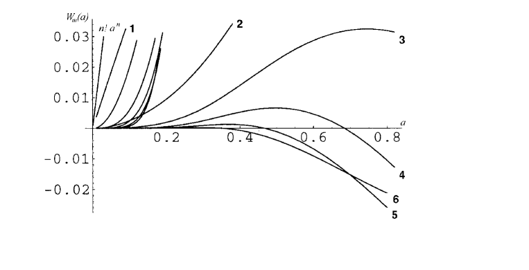
Figure 4: The functions $W_{m}(a)$ defined with the PV prescription (17), $m=1,\ldots 6$ for $a$ from $0$ to $0.8$. Unlabelled are the perturbative expansion functions $n!a^{n}$ for $n=1,\ldots,6$.

3.3 Asymptotic expansion of $W_{n}(a)$ for small $a$

In this subsection we investigate the perturbative expansion of the functions $W_{n}(a)$ in powers of $a$. As shown in the previous subsection, $W_{n}(a)$ have singularities at $a=0$, so their Taylor expansions around the origin will be divergent series. We take first $a$ real and positive. The asymptotic expansion is obtained by applying Watson’s lemma [38]. Specifically, we consider the Taylor expansion

$$w^{n}(u)=\sum\limits_{k=n}^{\infty}\xi_{k}^{(n)}u^{k}\,,$$ (35)

which is convergent for $|u|<1$. The sum begins with $k=n$ since, as follows from (11), the derivatives $(w^{n})^{(k)}(0)$ vanish for $k<n$ (in particular $\xi^{(n)}_{n}=(3/8)^{n}$). Choosing a positive number $X<1$, we can express $w^{n}(u)$ for $0\leq u\leq X$ as

$$w^{n}(u)=\sum\limits_{k=n}^{N}\xi_{k}^{(n)}u^{k}\,+R_{N}^{(n)}\,,$$ (36)

with a bounded remainder

$$|R_{N}^{(n)}|<M_{n}u^{N+1}\,.$$ (37)

We write now $W_{n}(a)$ as

$$W_{n}(a)={1\over a}\int\limits_{0}^{X}\,{\rm e}^{-u/a}\,w^{n}(u)\,{\rm d}u\,+{1\over a}\int\limits_{X}^{\infty}\,{\rm e}^{-u/a}\,w^{n}(u)\,{\rm d}u\,,$$ (38)

and insert in the first term the expansion (36). This gives

$$W_{n}(a)={1\over a}\int\limits_{0}^{X}\,{\rm e}^{-u/a}\,\,\sum\limits_{k=n}^{N}\xi_{k}^{(n)}u^{k}{\rm d}u\,+{M_{n}\over a}\int\limits_{0}^{X}\,{\rm e}^{-u/a}\,\theta_{n}u^{N+1}{\rm d}u\,+{1\over a}\int\limits_{X}^{\infty}\,{\rm e}^{-u/a}\,w^{n}(u)\,{\rm d}u\,,$$ (39)

where $|\theta_{n}|<1$. Since $|w^{n}(u)|<1$, the last term in (39) is bounded as

$$\bigg{|}1/a\int\limits_{X}^{\infty}\,{\rm e}^{-u/a}\,w^{n}(u)\,{\rm d}u\,\bigg{|}<{\rm e}^{-X/a}\,.$$ (40)

On the other hand, for fixed $k>0$ we have

$${1\over a}\int\limits_{0}^{X}\,{\rm e}^{-u/a}\,u^{k}{\rm d}u\,=k!a^{k}-{1\over a}\int\limits_{X}^{\infty}\,{\rm e}^{-u/a}\,u^{k}{\rm d}u\,.$$ (41)

In the last term we make the change of variable $u=X(1+y)$ and use the inequality $(1+y)^{k}\leq{\rm e}^{k\,y}$ for $k>0$ [38], which implies that the following estimates

$${1\over a}\int\limits_{X}^{\infty}\,{\rm e}^{-u/a}\,u^{k}{\rm d}u\,={X^{k+1}\over a}{\rm e}^{-X/a}\int\limits_{0}^{\infty}\,{\rm e}^{-Xy/a}\,(1+y)^{k}{\rm d}y\,\leq$$

$${X^{k+1}\over a}{\rm e}^{-X/a}\int\limits_{0}^{\infty}\,{\rm e}^{-y(X/a-k)}{\rm d}y={X^{k+1}\over a(X/a-k)}{\rm e}^{-X/a}\,,$$ (42)

are valid for fixed $k$ and small $a$. Therefore Eq. (41) can be written as

$${1\over a}\int\limits_{0}^{X}\,{\rm e}^{-u/a}\,u^{k}{\rm d}u\,=k!a^{k}\,+O\left({\rm e}^{-{X\over a}}\right)\,.$$ (43)

By using this estimate in (39) and taking into account the inequality (40), we obtain

$$W_{n}(a)=\sum\limits_{k=n}^{N}\xi_{k}^{(n)}k!a^{k}\,+{\tilde{M}}_{n}\,(N+1)!\,a^{N+1}+O\left({\rm e}^{-{X\over a}}\right)\,,$$ (44)

where ${\tilde{M}}_{n}$ is independent of $N$. One has therefore the asymptotic series

$$W_{n}(a)\sim\sum\limits_{k=n}^{\infty}\xi_{k}^{(n)}k!a^{k}\,,\quad a\to 0_{+}\,\,.$$ (45)

It is easy to extend the above arguments for complex values of $a$ in the right half-plane, $|\psi|\leq\pi/2-\delta$ with $\delta>0$.

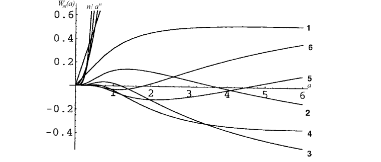
Figure 5: The same graph as in Fig. 4, with $a$ in the interval $(0,\,6)$.

The expansion (45) is independent of the prescription required in the definition of $W_{n}$. (It is formally obtained by inserting the expansion (35) in Eq. (15) and integrating term by term from 0 to $\infty$.) We notice that the first term of each $W_{n}(a)$ is proportional to $n!a^{n}$ with a positive coefficient, thereby retaining a fundamental property of perturbation theory. But the series (45) are divergent: indeed, since the expansions (35) have their convergence radii equal to 1, then for any $R>1$ there are infinitely many $k$ such that $|\xi^{(n)}_{k}|>R^{-k}$ [38]. Actually, the divergence of the series (45) is not surprising, in view of the analyticity properties derived in the previous section.

For illustration we give below the expansions of the first $W_{n}(a)$

$$W_{1}(a) \sim 0.375a-0.187a^{2}+0.457a^{3}-1.08a^{4}+4.32a^{5}+\ldots,$$

$$W_{2}(a) \sim 0.281a^{2}-0.422a^{3}+1.58a^{4}-5.80a^{5}+29.78a^{6}+\ldots,$$

$$W_{3}(a) \sim 0.316a^{3}-0.949a^{4}+5.04a^{5}-25.95a^{6}+167.99a^{7}+\ldots\,.$$ (46)

The higher powers of $a$ become quickly important in (46), the expansion coefficients eventually adopting factorial growth. For instance, the 5th-order coefficients in (46) all equal 5 approximately, while the 10th-order ones are between $5\times 10^{4}$ and $9\times 10^{4}$, with alternating signs. The functions $W_{n}(a)$ have divergent perturbative expansions, resembling the expanded QCD correlation function $D$.

Although the series (46) are divergent, the functions $W_{n}(a)$ are well-defined (once a prescription has been adopted), and bounded in the right half plane ${\rm Re}a>0$:

$$|W_{n}(a)|\leq\frac{1}{|a|}\int_{0}^{\infty}{\rm e}^{-u{\rm Re}a/|a|^{2}}|w^{n}(u)|{\rm d}u<{|a|\over{\rm Re}a}\,,$$ (47)

since $|w^{n}(u)|<1$. For $a$ real and positive the right hand side of (47) is equal to unity. We indicate in Figs. 4 and 5 the shape of the first functions $W_{n}$, calculated with the PV prescription, for real values of $a$.

3.4 Large-order behaviour of $W_{n}(a)$ and convergence conditions

The convergence of the series (14) is not a priori obvious. Indeed, the expansion (13) of the Borel transform in powers of $w$ converges for points $|w|<1$ arbitrarily close to the integration axis, but not necessarily on the boundary. Intuitively, one may expect that the convergence depends on the strength of the singularities of the Borel transform.

We investigated the convergence problem in [29], by estimating the behaviour of $W_{n}(a)$ for large $n$ with the method of steepest descent [36], [38]. The function $W_{n}^{(+)}(a)$ defined in (16) can be written as

$$W^{(\pm)}_{n}(a)=\int\limits_{{\cal C}_{\pm}}{\rm e}^{-F_{n}(u)}\,{\rm d}u\,,$$ (48)

where

$$F_{n}(u)={u\over a}-n\ln w(u)\,.$$ (49)

The saddle points of the integrand are given by the equation

$${w^{\prime}(u)\over w(u)}={1\over an}\,,$$ (50)

which has four complex solutions. The technique applied in [29] consists in rotating the integration axis in the complex $u$-plane, without crossing singularities, up to the nearest saddle points (located in the first (fourth) quadrant for ${\cal C}_{+}$ ( ${\cal C}_{-}$ ), respectively). Omitting the details given in [29], we quote the asymptotic behaviour of $W^{(+)}_{n}(a)$ for $n\rightarrow\infty$

$$W^{(+)}_{n}(a)\approx n^{{1\over 4}}\zeta^{n}{\rm e}^{-2^{3/4}(1+i){(n/a)^{1/2}}}\,,\quad n\to\infty\,,$$ (51)

with $\zeta$ defined below (12). Similarly, the large $n$ behaviour of $W^{(-)}_{n}(a)$ is

$$W^{(-)}_{n}(a)\approx n^{{1\over 4}}(\zeta^{*})^{n}{\rm e}^{-2^{3/4}(1-i){(n/a)^{1/2}}}\,,\quad n\to\infty\,.$$ (52)

These expressions are valid for complex $a$, $a=|a|{\rm e}^{{\rm i}\psi}$, where $\psi$ satisfies the inequality [29]

$$|\psi|<\pi/6\,.$$ (53)

The convergence of the expansion (14) depends on the ratio

$$\bigg{|}{c_{n}W^{(\pm)}_{n}(a)\over c_{n-1}W^{(\pm)}_{n-1}(a)}\bigg{|}\,.$$ (54)

As discussed in [28], if the coefficients $c_{n}$ satisfy the condition

$$|c_{n}|<C{\rm e}^{\epsilon n^{1/2}}\,$$ (55)

for any $\epsilon>0$, then the expansion (14) converges for $a$ complex in the domain

$${\rm Re}[(1\pm i)a^{-1/2}]>0\,,$$ (56)

which is equivalent to $|\psi|\leq\pi/2-\delta$. Since the condition (53) is more restrictive, it follows that, if the condition (55) is satisfied, the series (14) converges in the sector defined by (53).

The coefficients $c_{n}$ are obtained by inserting into the Taylor series (4) the expansions in powers of $w$ of the function $u(w)$ defined in (12). A precise estimate of the behaviour of the $c_{n}$ starting from a general form of the standard perturbative coefficients $D_{n}$ is difficult to obtain. In the special case of a Borel transform with branch point singularities, considered in [29], one can derive the generic behaviour

$$|c_{n}|\leq C^{\prime}n^{\xi}=C^{\prime}{\rm e}^{\xi\ln n}\,,\quad\xi>0\,,$$ (57)

which satisfies the convergence condition (55). Whether this bound is valid or not in general in QCD is an open problem, but (57) nevertheless represents a rather conservative assumption.

In subsection 3.2 we established analyticity properties for the functions $W_{n}(a)$ in the complex $a$ plane. The expanded function $D(s,a)$ will be holomorphic in the domain where the series (14) converges uniformly. Using the results of subsection 3.2, we conclude that $D(s,a)$ is expected to be holomorphic inside the sector (53) of the complex $a$-plane, with an essential singularity at the origin. This region is larger than the horn shaped domain found in [1] and [2]. The difference can be easily understood: indeed, the multiparticle singularities of the correlators in the momentum plane for $s\to\infty$, essential for the horn shaped boundaries preventing the analytic continuation near $a=0$ [1], [2], cannot appear in perturbative massless QCD, which is the frame adopted here.

4 Concluding remarks

In the present paper we used the analytic continuation in the Borel plane to define a modified perturbative expansion in QCD, the $n$-th order coefficient $c_{n}$ being calculable from the standard perturbative coefficients $D_{k}$, $k\leq n$. The new expansion functions $W_{n}(a)$ replacing the powers of the coupling constant are defined in (15) as the Laplace transforms of the $n$-th power of the function $w(u)$, which performs the conformal mapping of the whole doubly-cut Borel plane onto a unit disk.

The definition of the integral (15) is ambiguous due to the branch cut $u\geq 2$ along the integration path. We propose to define $W_{n}(a)$ by choosing the same prescription as that used to define the expanded function $D(s)$ itself, (6), so as to make the $W_{n}(a)$ resemble $D(s)$ as much as possible. The form of the $W_{n}(a)$ is not accidental or chosen ad hoc: it is imposed by the analyticity properties of the Borel transform, which in turn are determined by the information contained in the perturbative coefficients of the QCD correlation functions at all orders.

We proved that

/i/ the functions $W_{n}(a)$ are analytic in the complex $a$-plane, with essential and branch point singularities at $a=0$ (subsection 3.2),

/ii/ their expansions in powers of the coupling constant $a$ are asymptotic divergent series, the lowest order term of $W_{n}(a)$ being proportional to $a^{n}$ (subsection 3.3), and

/iii/ the expansion (14) of the correlation function in terms of the $W_{n}(a)$ set converges under plausible conditions, such that are expected to be satisfied in perturbative QCD (subsection 3.4, see also our previous paper [29]). By this we avoid the fatal divergence of the standard perturbative expansion: for the new expansion in terms of the $W_{n}(a)$, the addition of higher-order terms does not damage the result, as is the case with the series in powers of $a$. The convergence property is the main merit of the new expansion.

The prescription required for calculating the Laplace integral in the definition (15) reflects the intrinsic ambiguity of perturbation theory, which originates from the infrared regions of the Feynman diagrams and is manifest in the presence of the IR renormalon cut. Once a definition of the perturbative ambiguity is adopted (as the difference between two integration prescriptions, for instance), the series (14) provides a systematic calculation of this ambiguity at higher orders, since the expansion in terms of the $W_{n}(a)$ is convergent. This is to be contrasted with the standard expansion, where the ambiguity is defined in a less precise way by truncating the series at some finite order, beyond which the terms start to increase. Unlike in this procedure, the effects of the UV and IR parts of the Feynman diagrams have been disentangled in our approach.

Thus, using the analytic continuation in the Borel plane, we have been able to separate two problems that are usually interconnected: the divergence of the series (which can be solved within perturbation theory), and the problem of the intrinsic infrared ambiguity of perturbation theory. This ambiguity, expressed in the prescription dependence of the correlator and the expansion functions $W_{n}(a)$, can be removed only when nonperturbative effects are included.

Acknowledgements: The authors thank Prof. S. Randjbar-Daemi and the High Energy Section of the Abdus Salam International Centre for Theoretical Physics in Trieste for hospitality. One author (J.F.) is indebted to Prof. G. Altarelli for hospitality at the CERN Theory Division. Interesting discussions with Dr. Ivo Vrkoč on the mathematical aspects of this work (in particular his advice on the methods used in subsection 3.2) are gratefully acknowledged. This paper was partially supported by the Romanian Academy, under the Grant 49/2000, and by the Ministry of Industry and Trade of the Czech Republic, project RP-4210/69.

References

- [1] G. ’t Hooft, in: The Whys of Subnuclear Physics, Proceedings of the 15th International School on Subnuclear Physics, Erice, Sicily, 1977, edited by A. Zichichi (Plenum Press, New York, 1979), p. 943.
- [2] N. N. Khuri, Phys. Rev. D23, 2285 (1981).
- [3] V. Zakharov, Nucl.Phys. B385, 452 (1992).
- [4] A.H. Mueller, in QCD - Twenty Years Later, Aachen 1992, edited by P. Zerwas and H. A. Kastrup (World Scientific, Singapore, 1992).
- [5] M. Beneke and V. I. Zakharov, Phys. Lett. B312 340 (1993).
- [6] G. Grunberg, Phys. Lett. B 304, 183 (1993).
- [7] M. Beneke, Phys. Lett. B 307, 154 (1993); Nucl. Phys. B 405, 424 (1993).
- [8] D. Broadhurst, Z. Phys. C 58, 339 (1993).
- [9] R. Oehme, Newsletters, 7, 1 (1992); Int. J. Mod. Phys. A 10 1995 (1995),
- [10] K.A. Milton and I.L. Solovtsov, Phys.Rev. D 55, 5925 (1997).
- [11] D.V. Shirkov, Theor.Math.Phys.127 409-423 (2001).
- [12] P. M. Stevenson, Phys. Rev. D23, 2916 (1981).
- [13] G. Grunberg, Phys. Lett. B95, 70 (1980).
- [14] C. J. Maxwell, Phys.Lett. B409, 450 (1997).
- [15] M. A. Samuel, J. Ellis and M. Karliner, Phys. Rev. Lett. 74, 4389 (1995).
- [16] J. Ellis, M. Karliner and M.A. Samuel, Phys. Lett. B400, 197 (1997).
- [17] U.D. Jentschura, J. Becher, E. J. Weniger, G. Soff, Phys. Rev. Lett. 85, 2446 (2000).
- [18] P. Ball, M. Beneke and V.M. Braun, Nucl. Phys. B452, 563 (1995).
- [19] M. Neubert, Phys. Rev. D51, 5924 (1995).
- [20] C. N. Lovett-Turner and C. J. Maxwell, Nucl. Phys. B452, 188 (1995).
- [21] M. Beneke, Phys. Rep. 317, 1-142 (1999).
- [22] M. Beneke and V.M. Braun, hep-ph/0010208, Boris Ioffe Festschrift ”At the Frontier of Particle Physics/Handbook of QCD”, edited by M. Shifman (World Scientific, Singapore, 2001).
- [23] G.N. Hardy, Divergent Series (Oxford University Press, New York, 1949).
- [24] J. Fischer, Fortsch. Phys. 42, 665 (1994); Int. J.Mod.Phys. A 12, 3625 (1997).
- [25] A. Mueller, Nucl.Phys. B 250, 327 (1985).
- [26] G. Altarelli, P. Nason and G. Ridolfi, Z. Phys. C 68, 257 (1995).
- [27] D.E. Soper and L. R. Surguladze, Phys. Rev. D 54, 4566 (1996).
- [28] I. Caprini and J. Fischer, Phys.Rev D60, 054014 (1999).
- [29] I. Caprini and J. Fischer, Phys.Rev D62, 054007 (2000).
- [30] U.D. Jentschura, E. J. Weniger, G. Soff, J. Phys. G26, 1545 (2000).
- [31] G. Cvetič and T. Lee, Phys. Rev D54, 014030 (2001).
- [32] M. Beneke, V.M. Braun and N. Kivel, Phys. Lett. B 404, 315 (1997).
- [33] L.N.Lipatov, Sov.Phys. JETP 45, 216 (1977).
- [34] S. Ciulli and J. Fischer, Nucl. Phys. 24, 465 (1961).
- [35] I. Ciulli, S. Ciulli and J. Fischer, Nuovo Cim. 23, 1129 (1962).
- [36] J. Zinn-Justin, Quantum Field Theory and Critical Phenomena 2nd edition, (Oxford University Press, 1995), p. 923 - 928.
- [37] I. Caprini and M. Neubert, JHEP 03, 007 (1999).
- [38] H. Jeffreys, Asymptotic Approximations (Clarendon Press, Oxford, 1962).