Resummation of the QCD thermodynamic potential

Abstract

It is argued why thermodynamic approximations in terms of dressed propagators may, at larger coupling strength, be better behaved than perturbative results, and why in hot QCD the hard thermal loop approximation of the thermodynamic potential cannot be expected to work close to the phase transition.

1 Introduction

The thermodynamic potential is a quantity of central importance in statistical field theory, and a lot of interest has been devoted to its calculation. At high temperature, the perturbative expansion of the thermodynamic potential is known to 5th order in the coupling for the $\phi^{4}$ theory [1], [2], for QED [3], and for QCD [4], [5]. However, for physically relevant questions the applicability of these results is limited; they are meaningful only when the coupling is so weak that the thermodynamic potential is very close to its free limit. Already for moderate values of the coupling the accuracy of the approximation does not improve by the inclusion of higher order terms.

This feature of the perturbative expansion is similar to the behavior of asymptotic series. Consider, e. g., the integral $Z(g^{2})=\int_{-\infty}^{\infty}\!dx\exp\{-L\}$, where $L=\frac{1}{2}\,x^{2}+g^{2}x^{4}$, which may be seen as a caricature of the partition function ${\cal Z}$ in the $\phi^{4}$ theory [6]. $Z(g^{2})$ can be expressed in terms of a modified Bessel function. In the spirit of perturbation theory, however, one would expand the quartic ‘interaction part’ of the exponential, and perform the integrals before the sum to obtain an expansion in powers of $g^{2}$. Being related to the number of diagrams in the perturbative calculation of the partition function in the $\phi^{4}$ field theory, the coefficients of this series, $(-1)^{n}/n!\,\int\!dx\,x^{4n}\exp\{-x^{2}/2\}\sim(-1)^{n}n!$, alternate in sign and grow asymptotically like the factorial of the order $n$. Therefore, by the ratio test, the radius of convergence is zero. Nonetheless, the coefficients contain relevant information. In fact, the accuracy of the approximation of $Z(g^{2})$ by the truncated series does improve by higher-order terms as long as the truncation order is smaller than an optimal $n^{\star}\sim 1/g^{2}$.

The divergence of the perturbative expansion of $Z(g^{2})$ is obvious already in its definition: in the complex $g^{2}$ plane, $Z$ has a cut along the negative axis. Due to this essential feature one may presume that some of the properties of $Z(g^{2})$ and its expansion translate, at least qualitatively, to path integrals and, hence, to the thermodynamic potential $\Omega=-T\ln{\cal Z}$ in field theories. For example, the analysis of the (non-) convergence of the perturbative expansion of $\Omega$ demonstrates how the optimal truncation order decreases with increasing coupling. It is noted that for QCD close to the transition temperature already the next-to leading order perturbative contribution cannot be reconciled with the lattice data.

To motivate the following calculation of the thermodynamic potential in terms of the propagator, I want to point out another feature of the above toy model. Firstly, one can realize that the analog of the propagator, $d(g^{2})=\langle x^{2}\rangle/Z$, where the weight of the average is $\exp\{-L\}$, has also a cut along the negative $g^{2}$ axis. The same holds for the the ‘self-energy’ $p(g^{2})=d^{-1}(g^{2})-d^{-1}(0)$. This suggests to consider $Z$ as a complex function of $p$. It turns out that the mapping $p\rightarrow g^{2}\rightarrow Z$ unfolds the discontinuity along the negative $g^{2}$ axis. This analytic aspect is a formal motivation to choose, in the physics context, a representation of the thermodynamic potential in terms of the self-energy, or the dressed propagator, as a starting point to derive approximations. This is, of course, also supported by physical intuition. Dressed Greens functions are expected to be a preferable basis for nonperturbative approximations, since they resum entire subsets of ‘bare’ graphs. In particular, as known in other fields of physics, the excitations described by the full propagator may be considered as quasiparticles whose effective properties encode already a part of the interaction effects. The idea to understand the thermodynamics of a strongly coupled system in terms of its quasiparticles was successfully demonstrated for hot QCD in phenomenological models where the self-energies are approximated by their asymptotic values, see, e. g., [7].

In the following, a more systematic approach towards a quasiparticle description of the thermodynamics of field theories is given, starting from $\Phi$-derivable approximations. To outline this concept, the scalar theory is considered first in the next Section, before then turning to gauge theories.

2 $\Phi$-derivable approximations, scalar theory

The thermodynamic potential was first expressed as a functional of the exact propagator for a nonrelativistic fermion system [8]. This representation is the starting point for the so-called conserving approximation scheme [9], in which diagrams are resummed in thermodynamically consistent subsets. In the scalar theory, the thermodynamic potential can be expressed by the functional

$$\Omega[\Delta]=\frac{1}{2}\,\sum\int\,\left[\ln(-\Delta^{-1})+\Delta\Pi\right]-\Phi[\Delta]\,,$$ (1)

evaluated at its stationary point, $\delta\Omega/\delta\Delta=0$. This condition is equivalent to $\Pi/2=\delta\Phi/\delta\Delta$. It defines the full propagator $\Delta$, which is related to the self-energy $\Pi$ by Dyson’s equation, $\Delta^{-1}=\Delta_{0}^{-1}-\Pi$. $\Phi$ is given by the sum of the dressed 2-particle irreducible bubble diagrams; for the interaction $g_{0}^{2}/4!\,\phi^{4}$,

$$\Phi=3\;\raise-5.69054pt\hbox{\includegraphics[scale={0.55}]{c2.eps}}+12\;\raise-8.53581pt\hbox{\includegraphics[scale={0.35}]{baskb.eps}}+\ldots\,,$$ (2)

from which the expansion of $\Pi/2$ is obtained diagrammatically by cutting one line in each graph. The loop truncation of these skeleton expansions yields consistent (‘$\Phi$-derivable’) approximations [9].

At leading-loop order, the self-energy is just a mass term. The $\Phi$-derivable approximation can be obtained explicitly [11], and it is equivalent to the large-$N$ limit of the $O(N)$-symmetric scalar theory [12]. Considering, for simplicity, the massless theory, and working in $3-2\epsilon$ dimensions in the $\overline{MS}$ scheme, the self-energy is to be determined selfconsistently by

$$\Pi_{ll}=12\;\raise-4.2679pt\hbox{\includegraphics[scale={0.55}]{tadpole.eps}}\;=\frac{g_{0}^{2}}{2}\left(-\frac{\Pi_{ll}}{16\pi^{2}}\left[\frac{1}{\epsilon}-\ln\frac{\Pi_{ll}}{\bar{\mu}^{2}}+1\right]+\int_{k^{3}}\frac{n_{b}(\omega/T)}{\omega}\right)\,,\quad\mbox{where}\quad\omega=(k^{2}+\Pi_{ll})^{1/2}\,.$$ (3)

The right hand side contains a divergent contribution $\sim\Pi_{ll}/\epsilon$. This term, which implicitly depends on the temperature $T$, is the vacuum part of the resummed quantum fluctuations, while the medium contribution is finite due to the thermal distribution function $n_{b}$. The divergence is absorbed in the bare coupling constant. The renormalized coupling $g$ is defined as the scattering amplitude at a momentum scale $s$. Resumming the chains, $\includegraphics[scale={0.35}]{s.eps}\rule[-5.69054pt]{0.0pt}{18.49428pt}=\includegraphics[scale={0.35}]{s0.eps}+12\includegraphics[scale={0.35}]{s_l.eps}$, yields $g^{2}(s)=g_{0}^{2}-\frac{1}{2}g_{0}^{2}g^{2}(s)[1/\epsilon-\ln(-s/\bar{\mu}^{2})+2]/(16\pi^{2})$. Expressing now $g_{0}$ by $g$ renders eq. (3) finite and independent of $\bar{\mu}$,

$$\Pi_{ll}=\frac{g^{2}}{2}\left(\;\frac{\Pi_{ll}}{16\pi^{2}}\left[\ln\frac{\Pi_{ll}}{T^{2}}+1\right]+\int_{k^{3}}\frac{n_{b}(\omega/T)}{\omega}\right),$$ (4)

where the coupling $g$ has been defined at $-s=T^{2}$. This gap equation has a nontrivial structure. For $g$ smaller than $\tilde{g}\approx 10$, there are two solutions. The smaller one is related to the perturbative result which, by expanding the right hand side in $\Pi_{ll}/T^{2}$, is reproduced up to order $g^{3}$. The second solution, related to the tachyon [12], is for small $g^{2}$ exponentially large and thus of no physical relevance. As $g\rightarrow\tilde{g}$, the two solutions approach the same value, $\tilde{\Pi}=\Pi_{ll}(\tilde{g})\approx 4T^{2}$, and the leading-loop approximation can no longer be justified. For even larger values of the coupling, (4) has no solution.

At leading-loop order, the $\Phi$-contribution $\Phi_{ll}=\frac{1}{4}\,\hbox{$\Sigma$}\raise 1.00006pt\hbox{$\int$}\,\Pi_{ll}\Delta_{ll}$ combines with the first term in eq. (1),

$$\Omega_{ll}=\frac{1}{2}\,\sum\int\,\left[\ln(-\Delta_{ll}^{-1})+\textstyle\frac{1}{2}\displaystyle\,\Delta_{ll}\Pi_{ll}\right]=\int_{k^{3}}T\ln\left(1-\exp\{-\omega/T\}\right)-\frac{\Pi_{ll}}{4}\,\int_{k^{3}}\frac{n_{b}(\omega/T)}{\omega}-\frac{\Pi_{ll}^{2}}{128\pi^{2}}\,.$$ (5)

I emphasize the relative factor of $\frac{1}{2}$ between the two terms under the sum-integral; it ensures that the divergent $T$-dependent contributions of these terms cancel: $(\Pi_{ll}/8\pi)^{2}[-1/\epsilon+\frac{1}{2}\,2/\epsilon]=0$. The first integral in eq. (5) is the thermodynamic potential of a system of quasiparticles with mass $\Pi_{ll}^{1/2}$. Expanded in $\Pi_{ll}/T^{2}\sim g^{2}$, it over-includes the perturbative ${\cal O}(g^{2})$ term by a factor of two. This is compensated by the second integral – in fact, the approximation (5) reproduces the ${\cal O}(g^{3})$ result. The term $\sim\Pi_{ll}^{2}$ is a remnant of the resummed vacuum fluctuations. It leads to a minimum in the pressure, $p=-\Omega/V$, considered as a function of the self-energy, see Fig. 1. Due to the stationary property of $\Omega_{ll}$, the location of this minimum coincides with $\tilde{\Pi}_{ll}$, and hence indicates also where the leading-loop approximation breaks down.

This observation is interesting. With regard to the next section, assume we had solved the gap equation only perturbatively, to leading order: $\Pi_{ll}\approx\Pi^{\star}=(g_{0}T)^{2}/24$ (without resummation, the coupling remains bare). This is equivalent to the hard thermal loop (HTL) approximation of $\Pi$. Approximating now the $\Phi$-contribution by $\Phi^{\star}=\frac{1}{4}\,\hbox{$\Sigma$}\raise 1.00006pt\hbox{$\int$}\,\Pi^{\star}\Delta^{\star}$ yields the same functional form (5) for $\Omega^{\star}(\Pi^{\star})$ as in the selfconsistent approximation. Therefore, the maximal value of the self-energy, and hence for the coupling, beyond which the approximation cannot be meaningful (which could not be surmised from $\Pi^{\star}=(g_{0}T)^{2}/24$) can be inferred also from the HTL approximation $\Omega^{\star}(\Pi^{\star})$, which is important for a later argument.

Another useful thermodynamic quantity is the entropy density, $s=dp/dT$. In the leading-loop $\Phi$-derivable approximation, it can alternatively be obtained from a 1-loop functional of the dressed propagator [13], [14], which is not specific to the $\phi^{4}$ theory. In this case, the result is equivalent to the entropy of a system of quasiparticles with mass $\Pi_{ll}^{1/2}$ in the selfconsistent approximation, or $(\Pi^{\star})^{1/2}$ in the HTL approximation. Therefore, the entropy is a monotonously decreasing function of the quasiparticle mass, see Fig. 1. It shows, in contrast to the pressure, no sign of the breakdown of the approximation. This observation is consistent with the thermodynamic relation, since to reconstruct $p$ from $s$ one needs the $T$-dependence of the self-energy. It is also plausible on general grounds. While the pressure and the self-energy contain vacuum contributions, which become important at larger coupling, the entropy is determined only by thermal excitations.

3 Gauge theories, QCD

Aside from the technical complications to solve a set of coupled nonlocal Dyson equations selfconsistently, it may not be desired in gauge theories. In the $\Phi$-derivable approximation scheme, ‘bare’ diagrams of all orders in the coupling are grouped in subsets to preserve thermodynamic consistency. Since this procedure distinguishes the 2-point functions in the hierarchy of Greens functions, it cannot be expected to also preserve gauge invariance (unless solved exactly to all orders in the loop expansion). Another, technical, issue is how to accomplish the renormalization of resummed self-energies at finite temperature. Approximating the self-energies at leading order in the coupling makes the renormalization trivial. This would correspond to the considerations at the end of the Sec. 2, and lead to similar consequences. For example, only the leading order of the pressure could be reproduced upon expanding the resulting expression, while the (gauge dependent) higher order terms would not match the perturbative ones.

However, it turns out that approximating the self-energies by their HTL contributions, which are gauge invariant, suffices to resum the leading contributions. When calculating the thermodynamic potential, this additional approximation requires to account for the $\Phi$-contribution more carefully than in the $\phi^{4}$ theory. For simplicity of the argument, consider first the case of QED,

$$\textstyle\Omega=\frac{1}{2}\,{\rm Tr}\!\left[\,\ln(-D^{-1})+D\Pi\,\right]-{\rm Tr}\!\left[\,\ln(-S^{-1})+S\Sigma\,\right]-\Phi[D,S]\,,\qquad\Pi=2\,\delta\Phi/\delta D\,,\quad\Sigma=-\delta\Phi/\delta S\,,$$ (6)

where $D=(D_{0}^{-1}-\Pi)^{-1}$ is the photon propagator, and $S=(S_{0}^{-1}-\Sigma)^{-1}$ is the electron propagator. The Lorentz and spinor indices are implicit here, and summed over in the traces. At leading loop order,

$$\Phi_{ll}=\frac{1}{2}\includegraphics[scale={0.35}]{phi_qed.eps}\,,\quad\Pi_{ll}=\includegraphics[scale={0.35}]{se_b_qed.eps}\,,\quad\Sigma_{ll}=-\includegraphics[scale={0.35}]{se_f_qed.eps}\,.$$ (7)

Both in the selfconsistent and in the perturbative approximation, the $\Phi$-contribution to the thermodynamic potential could be evaluated by closing the external legs of, either, the photon or the electron self-energy, or a linear combination of those traces. This is not the case in the HTL approximation, where terms of order of the external momentum squared are neglected for the contributions $\sim T^{2}$. However, when traced over all momenta, these terms contribute to the same order, $e^{2}T^{4}$, as the HTL self-energies. This does not indicate that the HTL approximation is inutile here, but rather suggests the solution of this riddle, namely by keeping track of all relevant terms in $\Phi_{ll}$. At order $e^{2}$, $\Phi_{ll}$ is given by a double sum-integral over an expression with a numerator $N=K^{2}-Q_{1}^{2}-Q_{2}^{2}$, where $K$ is the photon momentum, and $Q_{1,2}$ are the electron momenta. One of the three terms in $N$ would be neglected in the HTL approximation, e. g., closing the legs of the photon HTL self-energy $\Pi^{\star}$ amounts to drop $K^{2}$. Summing over the cases where one of the terms in $N$ is dropped yields $2N$. Hence, $\Phi^{\star}=\frac{1}{4}\,{\rm Tr}\Pi^{\star}D^{\star}-\frac{1}{2}\,{\rm Tr}\Sigma^{\star}S^{\star}$ is equivalent to $\Phi_{ll}$ up to terms of higher order. The resulting approximation [15] for $\Omega$,

$$\textstyle\Omega^{\star}=\frac{1}{2}\,{\rm Tr}\!\big{[}\,\ln(-D^{\star\,-1})+\frac{1}{2}\,\Pi^{\star}D^{\star}\,\big{]}-{\rm Tr}\!\big{[}\,\ln(-S^{\star\,-1})+\frac{1}{2}\,\Sigma^{\star}S_{\star}\,\big{]},$$ (8)

is in close analogy (notice the factors $\frac{1}{2}$ in the trace terms) to the expression in the scalar theory.

For QCD, a similar (though due to the non-Abelian topology slightly more involved) analysis of the HTL $\Phi$-contribution was given in [15]. Let me here argue directly for a SU($N_{c})$ gluon plasma (including ghosts to compensate the unphysical degrees of freedom) why to expect the expression

$$\textstyle\Omega_{g}^{\star}=\frac{1}{2}\,{\rm Tr}_{c}\!\big{[}\,\ln(-D_{g}^{\star\,-1})+\frac{1}{2}\,\Pi_{g}^{\star}D_{g}^{\star}\,\big{]}-{\rm Tr}_{c}\!\big{[}\ln(-D_{ghost,0}^{-1})\big{]}\,.$$ (9)

The transverse and longitudinal components of the gluon HTL self-energy $\Pi^{\star}(p_{0},p)$ are given by dimensionless functions of $p_{0}/p$, times the asymptotic gluon mass squared, $M_{g}^{2}=\frac{1}{6}\,N_{c}\,g^{2}T^{2}$. Therefore, $M_{g}^{2}\partial_{M_{g}^{2}}\ln(-D_{g}^{\star\,-1})=-\Pi_{g}^{\star}D_{g}^{\star}$. Hence, the factor $\frac{1}{2}$ between the two terms in the gluon trace is indispensable to cancel their individually divergent contributions,

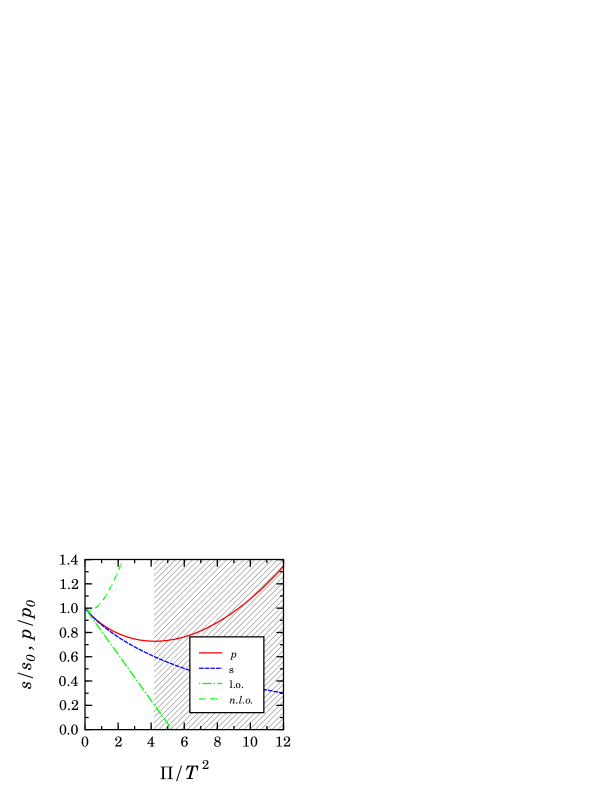
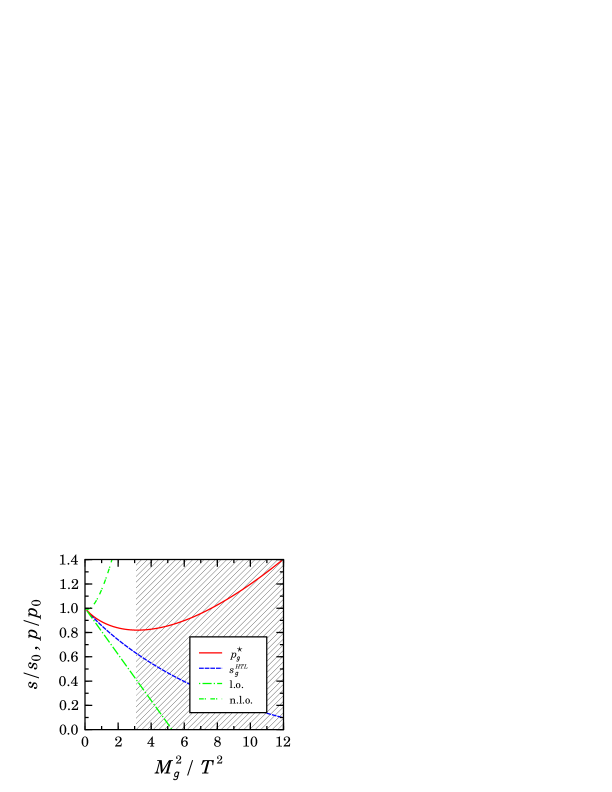
Figure 1: Pressure and entropy in the HTL approximation, as functions of the thermal mass scale in the $\phi^{4}$ theory (left), and for SU($N_{c}$) (right). Shown also are the leading and next-to leading perturbative results. In the $\phi^{4}$ theory, the selfconsistent and the HTL approximation have the same functional dependence on the respective self-energy. In the hatched region the approximations are not justified.

which are $\sim M_{g}^{4}/\epsilon^{n}$ on dimensional grounds. The result (9) has a striking similarity to the scalar case. Its expansion reproduces the ${\cal O}(g^{2})$ result, but under-estimates the ${\cal O}(g^{3})$ term by a factor of $\frac{1}{4}$. The pressure $p_{g}^{\star}$ has a minimum at $\tilde{M}_{g}^{2}\approx 3T^{2}$ (see Fig. 1). Similar to the $\phi^{4}$ theory, the dip is caused by a term $\sim M_{g}^{4}$ implicit in (9). It originates from the vacuum contributions, which for larger coupling become as important as the thermal contributions. This is in accordance with the general argumentation in Sec. 2, and not specific to the HTL approximation. I therefore conjecture also for QCD, where the solution structure of the selfconsistent Dyson equation cannot be studied explicitly, that the leading-loop approximation may not be meaningful for $M_{g}\mathrel{\hbox to0.0pt{\lower 1.99997pt\hbox{$\sim$}\hss}\raise 1.99997pt\hbox{$>$}}\tilde{M}_{g}$. Again, this could not be inferred from the HTL entropy $s_{g}^{{}_{HTL}}$ [14] which decreases monotonously with $M_{g}^{2}$. This conjecture is supported by lattice data.

Figure 2: The pressure as a function of the temperature in the SU(3) theory. The shaded band shows the lattice data [16], [17]. The hatched band for $p_{g}^{\star}$ represents the variation of the result when determining the temperature dependence of $M_{g}^{2}$ by, either, the 1- or the 2-loop running coupling in the $\overline{MS}$ scheme, assuming $T_{c}=1.14\Lambda_{\overline{MS}}$, and varying the renormalization scale $1\leq\bar{\mu}/(\pi T)\leq 4$ as in [14]. In accordance with the conjecture in the text (but not shown here), also the HTL entropy $s_{g}^{{}_{HTL}}(T)$ starts to deviate clearly from the lattice data below $3T_{c}$ [14].

At $\tilde{M}_{g}$, $p_{g}^{\star}$ is approximately 80% of the free pressure, a value reached by the lattice data at $3T_{c}$ ($T_{c}$ is the confinement temperature). At this temperature, indeed, $p_{g}^{\star}(T)$ starts to match the data, see Fig. 2, as does the entropy $s_{g}^{{}_{HTL}}$ [14].

In conclusion, it was shown that the HTL approximations of thermodynamic observables has a considerably improved range of applicability in the large coupling regime compared to perturbative results. For hot QCD, the approximation works down to temperatures of a few times above $T_{c}$. This encourages developments to extend, similar to the approach [18], the formalism to finite chemical potential, where no lattice data are available so far.

References

- [1] R. R. Parwani, H. Singh, Phys. Rev. D51, 4518 (1995).
- [2] E. Braaten, A. Nieto, Phys. Rev. D51, 6990 (1995).
- [3] R. R. Parwani, C. Coriano, Nucl. Phys. B434, 56 (1995).
- [4] C. Zhai, B. Kastening, Phys. Rev. D52, 7232 (1995).
- [5] E. Braaten, A. Nieto, Phys. Rev. D53, 3421 (1996).
- [6] C. Itzykson, J. B. Zuber, Quantum field theory, Mc Graw Hill (1980).
- [7] A. Peshier, B. Kämpfer, O. P. Pavlenko, G. Soff, Phys. Rev. D54, 2399 (1996).
- [8] J. M. Luttinger, J. C. Ward, Phys. Rev. 118, 1417 (1960).
- [9] G. Baym, Phys. Rev. 127, 1391 (1962).
- [10] F. Karsch, A. Patkos, P. Petreczky, Phys. Lett. B401, 69 (1997).
- [11] A. Peshier, B. Kämpfer, O. P. Pavlenko, G. Soff, Europhys. Lett. 43, 381 (1998).
- [12] I. T. Drummond, R. R. Horgan, P. V. Landshoff, A. Rebhan, Nucl. Phys. B524, 579 (1998).
- [13] B. Vanderheyden, G. Baym, J. Stat. Phys. 93, 843 (1998).
- [14] J. P. Blaizot, E. Iancu, A. Rebhan, Phys. Rev. Lett. 83, 2906 (1999); Phys. Rev. D63, 065003 (2001).
- [15] A. Peshier, Phys. Rev. D63, 105004 (2001).
- [16] G. Boyd et al., Nucl. Phys. B469, 419 (1996).
- [17] M. Okamoto et al., Phys. Rev. D60, 094510 (1999).
- [18] A. Peshier, B. Kämpfer, G. Soff, Phys. Rev. C61, 045203 (2000).