hep-ph/0110331 TTP01-23
NIKHEF 01-015
October 2001

Next-to-Next-to-Leading Order QCD Corrections
to the Photon’s Parton Structure
S. Moch${}^{\,a}$, J.A.M. Vermaseren${}^{\,b}$ and A. Vogt${}^{\,b}$
^aInstitut für Theoretische Teilchenphysik
Universität Karlsruhe, D–76128 Karlsruhe, Germany

^bNIKHEF Theory Group
Kruislaan 409, 1098 SJ Amsterdam, The Netherlands

Abstract

The next-to-next-to-leading order (NNLO) corrections in massless perturbative QCD are derived for the parton distributions of the photon and the deep-inelastic structure functions $F_{1}^{\,\gamma}$ and $F_{2}^{\,\gamma}$. We present the full photonic coefficient functions at order $\alpha\alpha_{\rm s}$ and calculate the first six even-integer moments of the corresponding ${\cal O}(\alpha\alpha_{\rm s}^{2})$ photon-quark and photon-gluon splitting functions together with the moments of the $\alpha\alpha_{\rm s}^{2}$ coefficient functions which enter only beyond NNLO. These results are employed to construct parametrizations of the splitting functions which prove to be sufficiently accurate at least for momentum fractions $x\,\raisebox{-1.9919pt}{$\>\stackrel{{\scriptstyle>}}{{{\scriptstyle\sim}}}\>$}\,0.05$. We also present explicit expressions for the transformation from the $\overline{\mbox{MS}}$ to the DIS_γ factorization scheme and write down the solution of the evolution equations. The numerical impact of the NNLO corrections is discussed in both schemes.

1 Introduction

The hadronic structure of the photon, in particular the deep-inelastic structure function $F_{2}^{\,\gamma}$, has attracted interest since the early days of perturbative QCD. Indeed, the leading-order (LO) corrections to the ‘pointlike’ parton-model result [1] were derived twenty-five years ago in ref. [2], and the next-to-leading order (NLO) contributions followed a few years later [3]. These results, obtained in the framework of the operator product expansion (OPE) [4], were recast in the language of evolution equations for the photon’s quark and gluon momentum distributions in refs. [5] and [6]. An error in the NLO photon-gluon anomalous dimension was corrected ten years ago [7, 8]. Unlike the case of lepton-nucleon deep-inelastic scattering (DIS) [9 – 15], the next-to-next-to-leading order (NNLO) QCD corrections have not been addressed for the photon structure up to now.

So far the measurements of $F_{2}^{\,\gamma}$ have been performed using the process $e^{+}e^{-}\!\rightarrow\!e^{+}e^{-}+{\it hadrons}\,$ at electron-positron colliders; see refs. [16] for recent overviews. While data from LEP have greatly improved the situation, an accuracy comparable to that achieved in lepton-hadron DIS can only be envisaged if $e\gamma$ collisions will be realized via laser back-scattering [17] of one of the electron beams of a future linear collider [18, 19]. Important information on the photon structure can also be expected from photoproduction of jets at HERA, which has been treated at NLO thus far [20 – 23]. The extension to NNLO is under way, e.g., the two-loop matrix element required also for hadronic collisions have been derived in refs. [24] using the pioneering results [25] for the scalar double box diagrams; the corresponding results with one external photon will be available soon [26].

In this article we present, with one qualification concerning the splitting functions, the NNLO corrections for electron-photon DIS and the evolution of the parton densities of the photon in massless perturbative QCD. In Sect. 2 we extend the OPE analysis of the photon structure [2, 3] to the required accuracy: The partonic forward amplitudes for the scattering of a virtual photon (and of a fictitious scalar directly coupled only to gluons) off a real photon are expressed in terms of the anomalous dimensions and coefficient functions up to second order in the strong coupling constant. Our calculation of these amplitudes for the lowest six even-integer values of the Mellin variable, $N=2,\,\ldots,\,12$, then facilitates the extraction of the corresponding anomalous dimensions (up to NNLO) and coefficient functions (up to the next-to-next-to-next-to-leading order, N³LO). The results for these quantities in the $\overline{\mbox{MS}}$ scheme are presented in Sect. 3 in numerical form, together with a brief discussion of the actual computation which closely followed the lines of refs. [11, 12]. The analytic expressions for these results can be found in Appendix A.

In Sect. 4 we switch to the parton language and specify the dependence of the photon-parton splitting functions and the photonic coefficient functions on the renormalization and factorization scales. After recalling the general factorization-scheme transformation, we then derive the NNLO corrections in the DIS_γ scheme [8] and discuss the ‘physical’ kernel for the non-singlet evolution of the structure functions at large values of the Bjorken variable $x$. The NNLO solution of the evolution equations is also given in this section. Explicit $x$-space expressions for the photonic coefficient functions and the photon-parton splitting functions up to NNLO are presented in Sect. 5. For the splitting functions we have to rely on our finite-$N$ results of Sect. 3, thus we can only provide approximations analogous to those derived in refs. [13, 14, 15] for the three-loop QCD splitting functions. For the NNLO coefficient functions and the corresponding transformation of the splitting functions to the DIS_γ scheme we present, besides the exact results (deferred to Appendix B for the latter quantities), also compact approximate expressions. In Sect. 6 we finally illustrate the numerical effect of the NNLO corrections on the evolution kernels and on the solution of the evolution equations. Our conclusions are presented in Sect. 7.

2 Moments: formalism and method

The subject of our calculation is inclusive hadron production in unpolarized electromagnetic (e.m.) deep-inelastic electron-photon scattering,

$$e(k)+\gamma(p)\>\rightarrow\>e(k^{\prime})+X\>\>,$$ (2.1)

where ‘$X$’ stands for all hadronic states allowed by quantum number conservation. The hadronic part of the corresponding amplitude is given by the (spin-averaged) tensor

$$W^{\,\gamma\Gamma}_{\mu\nu}(p,q) = \frac{1}{4\pi}\int\!d^{\,4}z\,e^{iq\cdot z}\,\langle\Gamma,p|\,J_{\mu}(z)J_{\nu}(0)\,|\Gamma,p\rangle$$ (2.2)

$$= e_{\mu\nu}\,\frac{1}{2x}F_{L}^{\,\gamma}(x,Q^{2})+d_{\mu\nu}\,\frac{1}{2x}F_{2}^{\,\gamma}(x,Q^{2})$$

with

$$e_{\mu\nu} = g_{\mu\nu}-\frac{q_{\mu}q_{\nu}}{q^{2}}$$

$$d_{\mu\nu} = -g_{\mu\nu}-p_{\mu}p_{\nu}\,\frac{4x^{2}}{q^{2}}-(p_{\mu}q_{\nu}+p_{\nu}q_{\mu})\,\frac{2x}{q^{2}}\>\>.$$ (2.3)

Here $|\Gamma,p\rangle$ denotes the physical photon state (including a non-perturbative hadronic component) with momentum $p$, and $J_{\mu}$ represents the e.m. quark current. $q=k-k^{\prime}$ is the momentum transferred by the electron, $Q^{2}=-q^{2}$, and $x=Q^{2}/(2p\cdot q)$ is the Bjorken variable ($0<x<1$). The longitudinal structure function $F_{L}$ is related to the structure function $F_{1}$ by $F_{L}=F_{2}-2xF_{1}$.

The optical theorem relates the tensor $W_{\mu\nu}$ in Eq. (2.2) to the forward amplitude $T_{\mu\nu}$ for the scattering of a virtual photon off a real photon,

$$T^{\,\gamma\Gamma}_{\mu\nu}(p,q)\>=\>i\!\int\!d^{\,4}z\,e^{iqz}\,\langle\Gamma,p|\,T\big{(}J_{\mu}(z)J_{\nu}(0)\big{)}\,|\Gamma,p\rangle\>\>.$$ (2.4)

This quantity represents a convenient starting point for practical calculations, due to the presence of the time-ordered product of currents to which standard perturbation theory applies. In fact, the operator product expansion for this product and the subsequent application of a dispersion relation to Eq. (2.4) very closely follow the procedure for standard lepton-hadron deep-inelastic scattering discussed, for example, in refs. [10, 11, 27] to which we refer the reader for details. In the leading-twist sector addressed in this article, the only, but crucial difference to the lepton-hadron case is the presence of the spin-$N$ twist-2 photon operators [2, 3]

$$O_{\gamma}^{\{\mu^{\,}_{1},\cdots,\mu^{\,}_{N}\}}\>=\>F^{\nu\{\mu^{\,}_{1}}D^{\mu^{\,}_{2}}\cdots D^{\mu^{\,}_{N-1}}F^{\mu^{\,}_{N}\}\nu}$$ (2.5)

and their coefficient functions $C_{i,\gamma}^{N}$ in addition to the usual quark (flavour non-singlet and singlet) and gluon operators, $O_{\rm ns}$, $O_{\rm q}$ and $O_{\rm g}$, and their respective coefficient functions. $D^{\mu}$ in Eq. (2.5) denotes the covariant derivative, and $F^{\mu\nu}$ represents the e.m. field strength tensor. The spin-averaged matrix elements of these (renormalized) operators are given by

$$\langle\Gamma,p|\,O_{\alpha}^{\{\mu^{\,}_{1},...,\mu^{\,}_{N}\}}\,|\Gamma,p\rangle\>=\>p^{\{\mu^{\,}_{1}}...p^{\mu^{\,}_{N}\}}\,A_{\,\Gamma,\alpha}^{N}(\mu^{2})\>\>,\quad\quad\alpha\,=\,\mbox{ns, q, g, }\gamma\>\>,$$ (2.6)

where $\mu$ stands for the renormalization scale. It is understood in Eqs. (2.5) and (2.6) that the symmetric and traceless part is taken with respect to the indices in curved brackets.

Following the procedure for lepton-hadron DIS [10, 11, 27], the even-integer Mellin-$N$ moments of the structure functions $F_{2}^{\,\gamma}$ and $F_{L}^{\,\gamma}$ in Eq. (2.2)

$$F_{i}^{\,\gamma,N}(Q^{2})\>=\>\int_{0}^{1}\!dx\,x^{N-1}{\cal F}_{i}^{\,\gamma}(x,Q^{2})\>\>,\quad\quad{\cal F}_{i}(x)=\frac{1}{x}\,F_{i}(x)$$ (2.7)

can then be expressed in terms of the parameters of the OPE,

$$F_{i}^{\,\gamma,N}(Q^{2})=\sum_{\alpha={\rm ns,q,g,}\gamma}C_{i,\alpha}^{N}\left(\frac{Q^{2}}{\mu^{2}},a_{\rm s},a_{\rm em}\right)A_{\,\Gamma,\alpha}^{N}(\mu^{2})\>\>,\quad\quad i=2,L\>\>.$$ (2.8)

Here and throughout the whole article we use the notation

$$a_{\rm s}\>=\>\frac{\alpha_{\rm s}}{4\pi}\>\>,\quad a_{\rm em}\>=\>\frac{\alpha}{4\pi}$$ (2.9)

for the strong and electromagnetic coupling constants. The present study addresses the higher-order QCD corrections to the photon structure functions $F_{2,L}^{\,\gamma}$ at the leading order of QED, $a_{\rm em}^{1}$. Consequently the quantities entering the r.h.s. of Eq. (2.8) are only needed at their respective lowest e.m. orders, i.e., $A_{\,\Gamma,\gamma}$ and $C_{i,\rm{p}}$ ($\rm{p=ns,q,g}$) at $a_{\rm em}^{0}$, and $A_{\,\Gamma,\rm{p}}$ and $C_{i,\gamma}$ at $a_{\rm em}^{1}$.

The operators $O_{\alpha}$ in Eq. (2.6) mix under renormalization. Expressing the renormalized operators in terms of their bare counterparts, this mixing can be written as

$$O_{\alpha}\>=\>Z_{\alpha\beta}\,O_{\beta}^{\rm bare}\>\>.$$ (2.10)

Here and in the next two equations the summation convention is used, and the range of all indices is as specified in Eq. (2.6) above. The anomalous dimensions $\gamma_{\alpha\beta}$ governing the scale dependence of the operators $O_{\alpha}$,

$$\frac{d}{d\ln\mu^{2}}\,O_{\alpha}\>=\>-\,\gamma_{\alpha\beta}\,O_{\beta}\>\>,$$ (2.11)

are connected to the mixing matrix $Z_{\alpha\beta}$ in Eq. (2.10) by

$$\gamma_{\alpha\beta}\>=\>-\,\left(\frac{d}{d\ln\mu^{2}}\,Z_{\alpha\alpha^{\prime}}\right)(Z^{-1})_{\alpha^{\prime}\beta}\>\>.$$ (2.12)

Keeping only those terms which are relevant for the structure functions $F_{2,L}^{\,\gamma}$ at order $a_{\rm em}^{1}$, the matrices $Z$ and $\gamma$ take the form

$$Z\>=\>\left(\begin{array}[]{cccc}Z_{\rm ns}&0&0&Z_{\rm ns\gamma}\\ 0&Z_{\rm qq}&Z_{\rm qg}&Z_{\rm q\gamma}\\ 0&Z_{\rm gq}&Z_{\rm gg}&Z_{\rm g\gamma}\\ 0&0&0&1\end{array}\right)$$ (2.13)

and

$$\gamma\>=\>\left(\begin{array}[]{cccc}\gamma_{\rm ns}&0&0&k_{\rm ns}\\ 0&\gamma_{\rm qq}&\gamma_{\rm qg}&k_{\rm q}\\ 0&\gamma_{\rm gq}&\gamma_{\rm gg}&k_{\rm g}\\ 0&0&0&0\end{array}\right)$$ (2.14)

with the perturbative expansions (where $k_{\rm g}^{(0)}=0$)

$$\gamma_{\rm p(p^{\prime})}\>=\>\sum_{l=0}^{\infty}\,a_{\rm s}^{l+1}\,\gamma_{\rm p(p^{\prime})}^{(l)}\>\>,\quad\quad k_{\rm{p}}\>=\>\sum_{l=0}^{\infty}\,a_{\rm em}\,a_{\rm s}^{l}\,k_{\rm{p}}^{(l)}\>\>.$$ (2.15)

In order to make practical use of Eq. (2.12) a regularization procedure and a renormalization scheme need to be selected. We choose dimensional regularization [28] and the modified [29] minimal subtraction [30] scheme, $\overline{\mbox{MS}}$ — the standard choice for modern multi-loop calculations in QCD. For this choice the running couplings in $D=4-2\epsilon$ dimensions evolve according to

$$\frac{d\,a_{j}}{d\ln\mu^{2}}\>=\>-\epsilon\,a_{j}+\beta_{j}(a_{j})\>\>,\quad\quad j=\mbox{em, s}\>\>,$$ (2.16)

where $\beta_{\rm em}$ and $\beta_{\rm s}$ denote the usual four-dimensional beta functions of QED and QCD, respectively. $\beta_{\rm em}$ does actually not enter the present calculation; for $\beta_{\rm s}$ we employ the standard notation

$$\beta_{\rm s}\>=\>-\beta_{0}\,a_{\rm s}^{2}-\beta_{1}\,a_{\rm s}^{3}-\beta_{2}\,a_{\rm s}^{4}-\ldots\>\>$$ (2.17)

with $\beta_{0}=11-2/3\,N_{\rm f}$, where $N_{\rm f}$ stands for the number of effectively massless quark flavours.

Inserting Eqs. (2.13)–(2.17) into Eq. (2.12) and solving for the photon-quark and photon-gluon renormalization factors $Z_{\rm ns\gamma}$, $Z_{\rm q\gamma}$ and $Z_{\rm g\gamma}$ we obtain, up to the desired order $a_{\rm em}a_{\rm s}^{2}$,

$$a_{\rm em}^{-1}\,Z_{\rm ns\gamma}\! = \frac{1}{\epsilon}\,k^{(0)}_{\rm ns}\,+\,a_{\rm s}\,\left[\frac{1}{\epsilon^{2}}\left\{\frac{1}{2}k^{(0)}_{\rm ns}\gamma^{(0)}_{\rm ns}\right\}+\frac{1}{2\epsilon}\,k^{(1)}_{\rm ns}\right]$$

$$\mbox{}+\,a_{\rm s}^{2}\,\left[\,\frac{1}{\epsilon^{3}}\left\{\frac{1}{6}k^{(0)}_{\rm ns}\left(\gamma^{(0)}_{\rm ns}\right)^{2}-\frac{1}{6}\beta_{0}k^{(0)}_{\rm ns}\gamma^{(0)}_{\rm ns}\right\}\right.$$

$$\quad\quad\>\mbox{}\left.+\frac{1}{\epsilon^{2}}\left\{\frac{1}{3}k^{(0)}_{\rm ns}\gamma^{(1)}_{\rm ns}+\frac{1}{6}k^{(1)}_{\rm ns}\gamma^{(0)}_{\rm ns}-\frac{1}{6}\beta_{0}k^{(1)}_{\rm ns}\right\}+\frac{1}{3\epsilon}\,k^{(2)}_{\rm ns}\right]\>\>,$$

$$a_{\rm em}^{-1}\,Z_{\rm q\gamma} = \frac{1}{\epsilon}\,k^{(0)}_{\rm{q}}\,+\,a_{\rm s}\,\left[\,\frac{1}{\epsilon^{2}}\left\{\frac{1}{2}k^{(0)}_{\rm q}\gamma^{(0)}_{\rm qq}\right\}+\frac{1}{2\epsilon}\,k^{(1)}_{\rm q}\right]$$

$$\mbox{}+\,a_{\rm s}^{2}\,\left[\,\frac{1}{\epsilon^{3}}\left\{\frac{1}{6}k^{(0)}_{\rm q}\left(\gamma^{(0)}_{\rm qq}\right)^{2}+\frac{1}{6}k^{(0)}_{\rm q}\gamma^{(0)}_{\rm qg}\gamma^{(0)}_{\rm gq}-\frac{1}{6}\beta_{0}k^{(0)}_{\rm q}\gamma^{(0)}_{\rm qq}\right\}\right.$$

$$\quad\quad\>\mbox{}\left.+\frac{1}{\epsilon^{2}}\left\{\frac{1}{3}k^{(0)}_{\rm q}\gamma^{(1)}_{\rm qq}+\frac{1}{6}k^{(1)}_{\rm q}\gamma^{(0)}_{\rm qq}+\frac{1}{6}k^{(1)}_{\rm g}\gamma^{(0)}_{\rm qg}-\frac{1}{6}\beta_{0}k^{(1)}_{\rm q}\right\}+\frac{1}{3\epsilon}\,k^{(2)}_{\rm q}\right]\>\>,$$

$$a_{\rm em}^{-1}\,Z_{\rm g\gamma} = \>+\>a_{\rm s}\>\left[\,\frac{1}{\epsilon^{2}}\left\{\frac{1}{2}k^{(0)}_{\rm q}\gamma^{(0)}_{\rm gq}\right\}+\frac{1}{2\epsilon}\,k^{(1)}_{\rm g}\right]$$

$$\mbox{}+\,a_{\rm s}^{2}\,\left[\,\frac{1}{\epsilon^{3}}\left\{\frac{1}{6}k^{(0)}_{\rm{q}}\gamma^{(0)}_{\rm gq}\left(\gamma^{(0)}_{\rm qq}+\gamma^{(0)}_{\rm gg}\right)-\frac{1}{6}\beta_{0}k^{(0)}_{\rm{q}}\gamma^{(0)}_{\rm gq}\right\}\right.$$

$$\quad\quad\>\mbox{}\left.+\frac{1}{\epsilon^{2}}\left\{\frac{1}{3}k^{(0)}_{\rm q}\gamma^{(1)}_{\rm gq}+\frac{1}{6}k^{(1)}_{\rm q}\gamma^{(0)}_{\rm gq}+\frac{1}{6}k^{(1)}_{\rm g}\gamma^{(0)}_{\rm gg}-\frac{1}{6}\beta_{0}k^{(1)}_{\rm g}\right\}+\frac{1}{3\epsilon}\,k^{(2)}_{\rm g}\right]\>\>.$$

The photon-parton anomalous dimensions $k_{\rm ns}$, $k_{\rm q}$ and $k_{\rm g}$ can thus be read off order-by-order from the $\epsilon^{-1}$ terms of the corresponding renormalization factors, while the higher poles in $1/\epsilon$ in Eqs. (2)–(2) can serve as checks for the calculation. The coefficient functions in Eq. (2.8), on the other hand, have an expansion in positive powers of $\epsilon$, viz

$$C_{i,\rm p} = \delta_{i2}\,(1-\delta_{\rm pg})+\sum_{l=1}^{\infty}\,a_{\rm s}^{l}\left(c_{i,\rm p}^{(l)}+\epsilon a_{i,\rm p}^{(l)}+\epsilon^{2}b_{i,\rm p}^{(l)}+\ldots\right)$$

$$C_{i,\gamma} = \sum_{l=1}^{\infty}\,a_{\rm em}\,a_{\rm s}^{l-1}\left(c_{i,\gamma}^{(l)}+\epsilon a_{i,\gamma}^{(l)}+\epsilon^{2}b_{i,\gamma}^{(l)}+\ldots\right)\>\>,$$ (2.21)

where $i=2,\,L$ and p = ns, q, g. Also here only the lowest-order terms in $a_{\rm em}$ have been retained as discussed below Eq. (2.8), thus, like the anomalous dimensions $\gamma_{\rm p(p^{\prime})}$ in Eq. (2.15), the coefficient functions $C_{i,\rm p}$ in Eq. (2) are just the standard QCD quantities entering lepton-hadron DIS.

Due to the partly non-perturbative physical photon state $|\Gamma,p\rangle$, Eqs. (2.4) and (2.8) are not accessible to a perturbative computation. However, as the OPE represents an operator relation, the anomalous dimensions (2.15) and the coefficient functions (2) do not depend on this state. Hence, again closely following the procedure [10, 11, 12] for lepton-nucleon DIS, the calculation can be performed using a partonic photon state $|\gamma,p\rangle$. Instead of Eq. (2.4) we thus consider

$$T^{\,\gamma\gamma}_{\mu\nu}(p,q)\>=\>i\!\int\!d^{\,4}z\,e^{iqz}\,\langle\gamma,p|\,T\big{(}J_{\mu}(z)J_{\nu}(0)\big{)}\,|\gamma,p\rangle\>\>.$$ (2.22)

At leading-twist accuracy the decomposition of $T^{\,\gamma\gamma}_{\mu\nu}$ into $T_{2,\gamma}$ and $T_{L,\gamma}$ analogous to Eq. (2.2) is provided by

$$T_{L,\gamma}(x,Q^{2}) = -\,\frac{q^{2}}{(p\cdot q)^{2}}\,p^{\mu}p^{\nu}\>T^{\,\gamma\gamma}_{\mu\nu}(p,q)$$

$$T_{2,\gamma}(x,Q^{2}) = -\left(\frac{3-2\epsilon}{2-2\epsilon}\>\frac{q^{2}}{(p\cdot q)^{2}}\,p^{\mu}p^{\nu}+\frac{1}{2-2\epsilon}\>g^{\mu\nu}\right)T^{\,\gamma\gamma}_{\mu\nu}(p,q)\>\>.$$ (2.23)

The $N^{\rm th}$ moments are obtained from Eqs. (2) by applying the projection operator ${\cal P}_{N}$ [31],

$$T^{N}_{i,\gamma}\left(\frac{Q^{2}}{\mu^{2}},a_{\rm s},a_{\rm em},\epsilon\right) = {\cal P}_{N}\,T_{i,\gamma}(x,Q^{2},a_{\rm s},a_{\rm em},\epsilon)$$

$$\equiv \left[\frac{q^{\{\mu_{1}}\cdots q^{\mu_{N}\}}}{N!}\,\frac{\partial^{N}}{\partial p^{\mu_{1}}\ldots\partial p^{\mu_{N}}}\right]\,T_{i,\gamma}(x,Q^{2},a_{\rm s},a_{\rm em},\epsilon)\Bigg{|}_{p=0}\>\>,$$

where $q^{\{\mu_{1}}\cdots q^{\mu_{N}\}}$ is the harmonic, i.e., the symmetric and traceless part of the tensor $q^{\mu_{1}}\cdots q^{\mu_{N}}$.

This operator does not act on the coefficient functions $C_{i,\alpha}$ and the renormalization constants $Z_{\alpha\beta}$ in Eq. (2.10), which are functions only of $N$, $\alpha_{\rm s}$, $\alpha$ and $\epsilon$. It does act, however, on the bare matrix elements $A_{\gamma,\alpha}^{N}$ (defined analogously to Eq. (2.6) ) and eliminates all diagrams containing loops, as the nullification of $p$ transform these diagrams to massless tadpole diagrams which are put to zero in dimensional regularization. This removes the operator matrix elements $A_{\gamma,\rm p}^{N}$, p = ns, q, g, which only start at the one-loop level. Hence only the matrix elements $A_{\gamma\gamma}^{N,\,\rm tree}$ of the photon operators (2.5) remain. These matrix elements are given by

$$A_{\gamma\gamma}^{N,\,\rm tree}(\epsilon)\>=\>(1-\epsilon)\cdot{\rm const}_{N}\>\>,$$ (2.25)

where the factor $(1-\epsilon)$ arises from the number of photon polarizations in $D=4-2\epsilon$ dimensions. We thus arrive at

$$T^{N}_{i,\gamma}\left(\frac{Q^{2}}{\mu^{2}},a_{\rm s},a_{\rm em},\epsilon\right)\>=\sum_{\alpha={\rm ns,q,g,}\gamma}C_{i,\alpha}^{N}\left(\frac{Q^{2}}{\mu^{2}},a_{\rm s},a_{\rm em},\epsilon\right)Z_{\alpha\gamma}^{N}\left(a_{\rm s},a_{\rm em},\frac{1}{\epsilon}\right)A_{\gamma\gamma}^{N,\,\rm tree}(\epsilon)$$ (2.26)

with $i=2,L$. This relation, after expanding in powers of $a_{\rm em}$, $a_{\rm s}$ and $\epsilon$, provides a system of coupled equations which can be solved for the photon-parton anomalous dimensions and the photon coefficient functions. In particular, by computing $T^{N}_{i,\gamma}$ to the order $a_{\rm em}\,a_{\rm s}^{2}$, we can derive the desired coefficients $k_{\rm ns}^{(2)N}$, $k_{\rm q}^{(2)N}$, and $c_{i,\gamma}^{(2)N}$ in Eqs. (2.15) and (2). The quantities $k_{\rm g}^{(2)N}$, on the other hand, cannot be determined in this manner since the gluonic coefficient function $C_{i,\rm g}$ in Eq. (2), unlike its quark counterparts, starts at order $a_{\rm s}$ only. This problem is overcome by considering, in addition to Eq. (2.22), another unphysical Green function $T^{\phi\gamma}$ where the virtual-photon probe is replaced by an external scalar field $\phi$ coupling directly only to gluons, see below.

The expansion of Eq. (2.26) to order $a_{\rm em}\,a_{\rm s}^{2}$ can be written as

$$T^{N}_{i,\gamma}\>=\>\sum_{l=0}^{2}\,a_{\rm em}\,a_{\rm s}^{l}\,S_{\epsilon}^{\,l+1}\bigg{(}\frac{\mu^{2}}{Q^{2}}\bigg{)}^{(l+1)\epsilon}T^{(l)N}_{i,\gamma}A_{\gamma\gamma}^{N,\,\rm tree}\>\>.$$ (2.27)

The factor $S_{\epsilon}=\exp\left[\epsilon\{\ln(4\pi-\gamma_{\rm E}\}\right]$, where $\gamma_{\rm E}$ denotes the Euler-Mascheroni constant, is an artefact of dimensional regularization kept out of the coefficient functions and anomalous dimensions in the $\overline{\mbox{MS}}$ scheme. The expansion coefficients $T^{(l)}_{i,\gamma}$ can be decomposed into flavour non-singlet (ns) and singlet (s) pieces,

$$T^{(l)}_{i,\gamma} = \delta_{\rm ns}\,T^{(l),\rm ns}_{i,\gamma}\,+\,\langle e^{2}\rangle\,\delta_{\rm s}\,T^{(l),\rm s}_{i,\gamma}$$

$$\equiv \delta_{\rm ns}\,T^{(l),\rm ns}_{i,\gamma}\,+\,\langle e^{2}\rangle\,\delta_{\rm s}\,\Big{(}T^{(l),\rm ns}_{i,\gamma}+T^{(l),\rm ps}_{i,\gamma}\Big{)}\>\>,$$

which collect the contributions proportional to the respective combinations of quark charges,

$$\delta_{\rm ns}\>=\>3N_{\rm f}\left(\langle e^{4}\rangle-\langle e^{4}\rangle^{2}\right)\>\>,\quad\quad\delta_{\rm s}\>\equiv\>\delta_{\rm q}\>=\>3N_{\rm f}\,\langle e^{2}\rangle\>\equiv\>3\,{\textstyle\sum_{j=1}^{N_{\rm f}}\,e_{q_{j}}^{2}}\>\>.$$ (2.29)

The pure-singlet (ps) contribution defined in the second line of Eq. (2) starts only at order $a_{\rm s}^{2}$. Consequently the anomalous dimensions $k^{(l)}_{\rm ns}$ and $k^{(l)}_{\rm q}$ in Eq. (2.15) are identical for $l\leq 1$ except for their obvious charge factors. The same applies, for $l\leq 2$, to the non-singlet and singlet photon coefficient functions in

$$c_{i,\gamma}^{(l)}\>=\>c_{i,\gamma}^{(l),\rm ns}+\langle e^{2}\rangle\,c_{i,\gamma}^{(l),\rm s}\>\>.$$ (2.30)

The corresponding decomposition for the hadronic quantities reads

$$\gamma_{\rm qq}^{(l)}\>=\>\gamma_{\rm ns}^{(l)}\>+\,\gamma_{\rm ps}^{(l)}\>\>,\quad\quad c_{i,\rm q}^{(l)}\>=\>c_{i,\rm ns}^{(l)}+\,c_{i,\rm ps}^{(l)}\>\>,$$ (2.31)

where the pure-singlet contributions are non-vanishing for $l\geq 1\>$(2) in the first (second) relation.

The explicit expressions for the first two singlet expansion coefficients in Eq. (2) in terms of the anomalous dimensions and coefficient functions are given by

$$\delta_{\rm s}T^{(0),\rm s}_{L,\gamma} = c^{(1),\rm s}_{L,\gamma}$$

$$\delta_{\rm s}\,T^{(0),\rm s}_{2,\gamma} = \frac{1}{\epsilon}\,k^{(0)}_{\rm q}+c^{(1),\rm s}_{2,\gamma}$$ (2.32)

and

$$\delta_{\rm s}\,T^{(1),\rm s}_{L,\gamma} = \,\frac{1}{\epsilon}\,\left\{k^{(0)}_{\rm{q}}c^{(1)}_{L,\rm q}\right\}+c^{(2),\rm s}_{L,\gamma}+k^{(0)}_{\rm q}a^{(1)}_{L,\rm q}$$

$$\delta_{\rm s}\,T^{(1),\rm s}_{2,\gamma} = \frac{1}{\epsilon^{2}}\left\{\frac{1}{2}k^{(0)}_{\rm q}\gamma^{(0)}_{\rm qq}\right\}+\frac{1}{\epsilon}\left\{\frac{1}{2}k^{(1)}_{\rm q}+k^{(0)}_{\rm q}c^{(1)}_{2,\rm q}\right\}+c^{(2),\rm s}_{2,\gamma}+k^{(0)}_{\rm{q}}a^{(1)}_{2,\rm q}\>\>.$$ (2.33)

The corresponding non-singlet relations are obvious as discussed below Eq. (2.29), hence they are not written out for brevity. The contributions at the order $a_{\rm em}\,a_{\rm s}^{2}$ read

$$\delta_{\rm ns}\,T^{(2),\rm ns}_{L,\gamma} = \frac{1}{\epsilon^{2}}\left\{\frac{1}{2}k^{(0)}_{\rm ns}\gamma^{(0)}_{\rm qq}c^{(1)}_{L,\rm q}\right\}+\frac{1}{\epsilon}\left\{k^{(0)}_{\rm ns}c^{(2)}_{L,\rm ns}+\frac{1}{2}k^{(1)}_{\rm ns}c^{(1)}_{L,\rm q}+\frac{1}{2}k^{(0)}_{\rm ns}\gamma^{(0)}_{\rm qq}a^{(1)}_{L,\rm q}\right\}$$

$$\mbox{}+c^{(3),\rm ns}_{L,\gamma}+k^{(0)}_{\rm ns}a^{(2)}_{L,\rm ns}+\frac{1}{2}k^{(1)}_{\rm ns}a^{(1)}_{L,\rm q}+\frac{1}{2}k^{(0)}_{\rm ns}\gamma^{(0)}_{\rm qq}b^{(1)}_{L,\rm q}\>\>,$$

$$\delta_{\rm ns}\,T^{(2),\rm{ns}}_{2,\gamma} = \quad\!\frac{1}{\epsilon^{3}}\left\{\frac{1}{6}k^{(0)}_{\rm ns}\left(\gamma^{(0)}_{\rm qq}\right)^{2}-\frac{1}{6}\beta_{0}k^{(0)}_{\rm ns}\gamma^{(0)}_{\rm qq}\right\}$$ (2.34)

$$\mbox{}\!\!+\frac{1}{\epsilon^{2}}\left\{\frac{1}{2}k^{(0)}_{\rm ns}\gamma^{(0)}_{\rm qq}c^{(1)}_{2,\rm q}+\frac{1}{3}k^{(0)}_{\rm ns}\gamma^{(1)}_{\rm ns}+\frac{1}{6}k^{(1)}_{\rm ns}\gamma^{(0)}_{\rm qq}-\frac{1}{6}\beta_{0}k^{(1)}_{\rm ns}\right\}$$

$$\mbox{}\!\!+\,\frac{1}{\epsilon}\>\left\{\frac{1}{3}k^{(2)}_{\rm ns}+k^{(0)}_{\rm ns}c^{(2)}_{2,\rm ns}+\frac{1}{2}k^{(1)}_{\rm ns}c^{(1)}_{2,\rm q}+\frac{1}{2}k^{(0)}_{\rm ns}\gamma^{(0)}_{\rm qq}a^{(1)}_{2,\rm q}\right\}$$

$$\mbox{}\!\!+\>c^{(3),\rm ns}_{2,\gamma}+k^{(0)}_{\rm ns}a^{(2)}_{2,\rm ns}+\frac{1}{2}k^{(1)}_{\rm ns}a^{(1)}_{2,\rm q}+\frac{1}{2}k^{(0)}_{\rm ns}\gamma^{(0)}_{\rm qq}b^{(1)}_{2,\rm q}$$

and

$$\delta_{\rm s}\,T^{(2),\rm ps}_{L,\gamma} = \frac{1}{\epsilon^{2}}\left\{\frac{1}{2}k^{(0)}_{\rm q}\gamma^{(0)}_{\rm{gq}}c^{(1)}_{L,\rm g}\right\}+\frac{1}{\epsilon}\left\{k^{(0)}_{\rm q}c^{(2)}_{L,\rm ps}+\frac{1}{2}k^{(1)}_{\rm g}c^{(1)}_{L,{\rm g}}+\frac{1}{2}k^{(0)}_{\rm q}\gamma^{(0)}_{\rm gq}a^{(1)}_{L,\rm g}\right\}$$

$$\mbox{}+c^{(3),{\rm ps}}_{L,\gamma}+k^{(0)}_{\rm q}a^{(2)}_{L,{\rm ps}}+\frac{1}{2}k^{(1)}_{\rm g}a^{(1)}_{L,{\rm g}}+\frac{1}{2}k^{(0)}_{\rm q}\gamma^{(0)}_{\rm gq}b^{(1)}_{L,\rm g}\>\>,$$

$$\delta_{\rm s}\,T^{(2),\rm ps}_{2,\gamma} = \frac{1}{\epsilon^{3}}\left\{\frac{1}{6}k^{(0)}_{\rm q}\gamma^{(0)}_{\rm qg}\gamma^{(0)}_{\rm gq}\right\}+\frac{1}{\epsilon^{2}}\left\{\frac{1}{2}k^{(0)}_{\rm{q}}\gamma^{(0)}_{\rm gq}c^{(1)}_{2,\rm g}+\frac{1}{6}k^{(1)}_{\rm g}\gamma^{(0)}_{\rm qg}+\frac{1}{3}k^{(0)}_{\rm q}\gamma^{(1)}_{\rm ps}\right\}$$ (2.35)

$$\mbox{}+\frac{1}{\epsilon}\left\{\frac{1}{3}k^{(2)}_{\rm ps}+k^{(0)}_{\rm q}c^{(2)}_{2,{\rm ps}}+\frac{1}{2}k^{(1)}_{\rm g}c^{(1)}_{2,{\rm g}}+\frac{1}{2}k^{(0)}_{\rm q}\gamma^{(0)}_{\rm gq}a^{(1)}_{2,\rm g}\right\}$$

$$\mbox{}+\,c^{(3),\rm ps}_{2,\gamma}+k^{(0)}_{\rm{q}}a^{(2)}_{2,{\rm ps}}+\frac{1}{2}k^{(1)}_{\rm g}a^{(1)}_{2,{\rm g}}+\frac{1}{2}k^{(0)}_{\rm q}\gamma^{(0)}_{\rm gq}b^{(1)}_{2,\rm g}\>\>.$$

Finally we derive the corresponding expressions for the unphysical flavour-singlet Green function $T^{\phi\gamma}(p,q)$ mentioned below Eq. (2.26). After application of the projection operator ${\cal P}_{N}$ in Eq. (2) the moments of $T^{\phi\gamma}$ can be written as

$$T^{N}_{\phi,\gamma}\left(\frac{Q^{2}}{\mu^{2}},a_{\rm s},a_{\rm em},\epsilon\right)\>=\sum_{\alpha={\rm q,g,}\gamma}C_{\phi,\alpha}^{N}\left(\frac{Q^{2}}{\mu^{2}},a_{\rm s},a_{\rm em},\epsilon\right)Z_{\alpha\gamma}^{N}\left(a_{\rm s},a_{\rm em},\frac{1}{\epsilon}\right)A_{\gamma\gamma}^{N,\,\rm tree}(\epsilon)\>\>.$$ (2.36)

The coefficient functions $C_{\phi,\alpha}$ have an expansion analogous to Eq. (2), but with $C_{\phi,\rm g}={\cal O}(1)$ and $C_{\phi,\rm q}={\cal O}(a_{\rm s})$. It is understood in Eq. (2.36) that the external gluon operator $G_{\mu\nu}G^{\mu\nu}$ employed for the coupling to the scalar field $\phi$ has been renormalized according to [32]

$$G^{\mu\nu}G_{\mu\nu}\>=\>Z_{G^{2}}\,\left(G^{\mu\nu}G_{\mu\nu}\right)^{\rm bare}\,+\,\ldots\>\>,\quad\quad Z_{G^{2}}\>=\>\frac{1}{1-\beta(\alpha_{\rm s})/(\epsilon\alpha_{\rm s})}\>\>,$$ (2.37)

where the dots indicate mixing with unphysical operators which give vanishing contributions under the conditions of the present calculation. Expanding Eq. (2.36) analogously to Eq. (2.27), the coefficients $T_{\phi,\gamma}^{(l)}$, $l=1,2$ read

$$T^{(1)}_{\phi,\gamma}\>=\>\frac{1}{\epsilon^{2}}\left\{\frac{1}{2}k^{(0)}_{\rm{q}}\gamma^{(0)}_{\rm gq}\right\}+\frac{1}{\epsilon}\left\{\frac{1}{2}k^{(1)}_{\rm g}+k^{(0)}_{\rm q}c^{(1)}_{\phi,\rm q}\right\}+c^{(2)}_{\phi,\gamma}+k^{(0)}_{\rm q}a^{(1)}_{\phi,\rm q}$$ (2.38)

and

$$T^{(2)}_{\phi,\gamma} \!=\! \>\frac{1}{\epsilon^{3}}\left\{\frac{1}{6}k^{(0)}_{\rm q}\gamma^{(0)}_{\rm gq}\left(\gamma^{(0)}_{\rm qq}+\gamma^{(0)}_{\rm gg}\right)-\frac{1}{6}\beta_{0}k^{(0)}_{\rm q}\gamma^{(0)}_{\rm gq}\right\}$$ (2.39)

$$\mbox{}\!\!\!\!\!\!+\frac{1}{\epsilon^{2}}\left\{\frac{1}{2}k^{(0)}_{\rm q}\gamma^{(0)}_{\rm gq}c^{(1)}_{\phi,\rm g}+\frac{1}{2}k^{(0)}_{\rm q}\gamma^{(0)}_{\rm qq}c^{(1)}_{\phi,\rm q}+\frac{1}{3}k^{(0)}_{\rm q}\gamma^{(1)}_{\rm gq}+\frac{1}{6}k^{(1)}_{\rm q}\gamma^{(0)}_{\rm gq}+\frac{1}{6}k^{(1)}_{\rm g}\gamma^{(0)}_{\rm gg}-\frac{1}{6}\beta_{0}k^{(1)}_{\rm g}\right\}$$

$$\mbox{}\!\!\!\!\!\!+\>\frac{1}{\epsilon}\,\left\{\frac{1}{3}k^{(2)}_{\rm{g}}+k^{(0)}_{\rm q}c^{(2)}_{\phi,{\rm q}}+\frac{1}{2}k^{(1)}_{\rm g}c^{(1)}_{\phi,{\rm g}}+\frac{1}{2}k^{(1)}_{\rm q}c^{(1)}_{\phi,{\rm q}}+\frac{1}{2}k^{(0)}_{\rm q}\gamma^{(0)}_{\rm gq}a^{(1)}_{\phi,\rm g}+\frac{1}{2}k^{(0)}_{\rm q}\gamma^{(0)}_{\rm qq}a^{(1)}_{\phi,\rm q}\right\}\>.\quad\quad$$

In Eq. (2.39) we have not written out the $\epsilon^{0}$ term fixing the unphysical coefficient function $c^{(3)}_{\phi,\gamma}$.

3 Moments: calculation and results

The calculation of the moments (2.26) and (2.36) of the Green functions $T^{\,\gamma\gamma}$ and $T^{\phi\gamma}$ can be performed quite analogously to that of $T^{\,\gamma\rm g}$ and $T^{\,\phi\rm g}$ in refs. [11, 12] (where these quantities are denoted as $T^{\rm g\gamma g\gamma}$ and $T^{\rm g\phi g\phi}$), to which the reader is referred for a more detailed discussion. Indeed, the Feynman diagrams contributing to $T^{\,\gamma\gamma}$ ($T^{\phi\gamma}$) derive from a subset of those for $T^{\,\gamma\rm g}$ ($T^{\phi\rm g}$): at three loops 117 (57) out of 366 (7162) diagrams contribute, respectively, using the counting of refs. [11, 12]. Despite this reduction we are not able to compute higher moments than obtained for the hadronic case in ref. [12], as some of the most storage-consuming diagrams remain.

The moments $N=2,\,\ldots,\,8$ have been calculated from scratch. The diagrams are generated using a special version of QGRAF [33]. The actual computation is done using optimized FORM [34] programs using the MINCER package [35] for the scalar three-loop integrals. The moments $N=2,4$ of $T^{\,\gamma\gamma}$ and $N=2$ of $T^{\,\phi\gamma}$ have been computed in an arbitrary covariant gauge, i.e., keeping the gauge parameter $\xi$ in the gluon propagator, $i\,[-g^{\mu\nu}+(1-\xi)q^{\mu}q^{\nu}/(q^{2}+i\epsilon)]/(q^{2}+i\epsilon)$ as a free parameter. The explicit cancellation of the gauge dependence in the anomalous dimensions and coefficient functions provides an important check of the results. The direct calculation of the moments $N\!=\!10$ and $N\!=\!12$ is rather time-consuming and requires running FORM on a computer with 64-bit architecture instead on a standard PC [12]. Therefore we have for these moments (and as a further check also for the lower moments) made use of the diagram database of ref. [12] by replacing the colour factors of $T^{\,\gamma\rm g}$ and $T^{\,\phi\rm g}$ by those for our cases and then re-assembling the integrated results of all diagrams, thus sidestepping the involved parts of the computation.

From the results of these calculations the ${\cal O}(a_{\rm em}a_{\rm s}^{2})$ photon-parton anomalous dimensions and photon coefficient functions at $N=2,\,\ldots,\,12$ can be obtained by means of Eqs. (2.27), (2), (2)–(2) and (2.38)–(2.39). Here we present the results in numerical form; the full analytic expressions can be found in Appendix A. The non-singlet ($\rm p=ns$) and singlet ($\rm p=s$) photon-quark anomalous dimensions read

$$(\delta_{\rm p}\,a_{\rm em})^{-1}\,k_{\rm p}^{N=2} = \mbox{}-1.333333333\>\>-a_{\rm s}\>7.308641975$$

$$\mbox{}+a_{\rm s}^{2}\,(\,-3.368998628\,f_{\rm ps}\,N_{\rm f}-86.97527479+1.470507545\,N_{\rm f}\,)$$

$$(\delta_{\rm p}\,a_{\rm em})^{-1}\,k_{\rm p}^{N=4} = \mbox{}-0.7333333333-a_{\rm s}\>8.343259259$$

$$\mbox{}+a_{\rm s}^{2}\,(\,-0.4223537997\,f_{\rm ps}\,N_{\rm f}-102.8310333+1.477370645\,N_{\rm f}\,)$$

$$(\delta_{\rm p}\,a_{\rm em})^{-1}\,k_{\rm p}^{N=6} = \mbox{}-0.5238095238-a_{\rm s}\>8.525587590$$

$$\mbox{}+a_{\rm s}^{2}\,(\,-0.1483655726\,f_{\rm ps}\,N_{\rm f}-109.2777760+1.656530217\,N_{\rm f}\,)$$

$$(\delta_{\rm p}\,a_{\rm em})^{-1}\,k_{\rm p}^{N=8} = \mbox{}-0.4111111111-a_{\rm s}\>8.343215919$$

$$\mbox{}+a_{\rm s}^{2}\,(\,-0.06961022336\,f_{\rm ps}\,N_{\rm f}-111.1669036+1.695497529\,N_{\rm f}\,)$$

$$(\delta_{\rm p}\,a_{\rm em})^{-1}\,k_{\rm p}^{N=10}\!\! = \mbox{}-0.3393939394-a_{\rm s}\>8.045400445$$

$$\mbox{}+a_{\rm s}^{2}\,(\,-0.03823222708\,f_{\rm ps}\,N_{\rm f}-111.0346700+1.670607074\,N_{\rm f}\,)$$

$$(\delta_{\rm p}\,a_{\rm em})^{-1}\,k_{\rm p}^{N=12}\!\! = \mbox{}-0.2893772894-a_{\rm s}\>7.720564967$$

$$\mbox{}+a_{\rm s}^{2}\,(\,-0.02324832852\,f_{\rm ps}\,N_{\rm f}-109.9430144+1.619078961\,N_{\rm f}\,)\>\>,\quad$$

where the factors $\delta_{\rm ns}$ and $\delta_{\rm s}$ have been defined in Eq. (2.29), and

$$f_{\rm ps}\>\equiv\>\left\{\begin{array}[]{l}0\>\>,\quad\quad{\rm p=ns}\\ 1\>\>,\quad\quad{\rm p=s}\>\>.\end{array}\right.$$ (3.2)

The corresponding results for the photon-gluon anomalous dimensions are given by

$$(\delta_{\rm s}\,a_{\rm em})^{-1}\,k_{\rm g}^{N=2} = a_{\rm s}\>1.975308642\>\>\>+\,a_{\rm s}^{2}\,(\,31.41971923+5.157750343\,N_{\rm f}\,)$$

$$(\delta_{\rm s}\,a_{\rm em})^{-1}\,k_{\rm g}^{N=4} = a_{\rm s}\>0.8743703704\,+\,a_{\rm s}^{2}\,(\,23.94271102+1.108863649\,N_{\rm f}\,)$$

$$(\delta_{\rm s}\,a_{\rm em})^{-1}\,k_{\rm g}^{N=6} = a_{\rm s}\>0.4439549365\,+\,a_{\rm s}^{2}\,(\,15.65166504+0.6959529917\,N_{\rm f}\,)$$

$$(\delta_{\rm s}\,a_{\rm em})^{-1}\,k_{\rm g}^{N=8} = a_{\rm s}\>0.2669916389\,+\,a_{\rm s}^{2}\,(\,10.96606146+0.4981961912\,N_{\rm f}\,)$$

$$(\delta_{\rm s}\,a_{\rm em})^{-1}\,k_{\rm g}^{N=10}\!\! = a_{\rm s}\>0.1780490673\,+\,a_{\rm s}^{2}\,(\,8.160308004+0.3790604508\,N_{\rm f}\,)$$ (3.3)

$$(\delta_{\rm s}\,a_{\rm em})^{-1}\,k_{\rm g}^{N=12}\!\! = a_{\rm s}\>0.1271644566\,+\,a_{\rm s}^{2}\,(\,6.348294844+0.3002739601\,N_{\rm f}\,)\>\>.\quad$$

For the scale choice $\mu^{2}=Q^{2}$ the photon coefficient functions for $F_{2}$ and $F_{L}$ at $N=2,\,\ldots,\,12$ read

$$(\delta_{\rm p}\,a_{\rm em})^{-1}\,c_{2,\gamma}^{\,{\rm p},N=2} = \mbox{}-1\>\>-a_{\rm s}\>5.54162471$$

$$\mbox{}+a_{\rm s}^{2}\,(\,-5.818386905\,f_{\rm ps}\,N_{\rm f}-83.61538634+12.00984563\,N_{\rm f}\,)$$

$$(\delta_{\rm p}\,a_{\rm em})^{-1}\,c_{2,\gamma}^{\,{\rm p},N=4} = \mbox{}-1.477777778-a_{\rm s}\>12.20420558$$

$$\mbox{}+a_{\rm s}^{2}\,(\,-12.34431320\,f_{\rm ps}\,N_{\rm f}-270.6890263+22.99272397\,N_{\rm f}\,)$$

$$(\delta_{\rm p}\,a_{\rm em})^{-1}\,c_{2,\gamma}^{\,{\rm p},N=6} = \mbox{}-1.410317460-a_{\rm s}\>16.88045086$$

$$\mbox{}+a_{\rm s}^{2}\,(\,-10.77343760\,f_{\rm ps}\,N_{\rm f}-461.1411168+31.41856945\,N_{\rm f}\,)$$

$$(\delta_{\rm p}\,a_{\rm em})^{-1}\,c_{2,\gamma}^{\,{\rm p},N=8} = \mbox{}-1.288174603-a_{\rm s}\>19.73136088$$

$$\mbox{}+a_{\rm s}^{2}\,(\,-8.964615998\,f_{\rm ps}\,N_{\rm f}-617.8190552+37.24672336\,N_{\rm f}\,)$$

$$(\delta_{\rm p}\,a_{\rm em})^{-1}\,c_{2,\gamma}^{\,{\rm p},N=10}\!\! = \mbox{}-1.172255892-a_{\rm s}\>21.44335073$$

$$\mbox{}+a_{\rm s}^{2}\,(\,-7.480750665\,f_{\rm ps}\,N_{\rm f}-741.1418081+41.20962391\,N_{\rm f}\,)$$

$$(\delta_{\rm p}\,a_{\rm em})^{-1}\,c_{2,\gamma}^{\,{\rm p},N=12}\!\! = \mbox{}-1.071686118-a_{\rm s}\>22.46033065$$

$$\mbox{}+a_{\rm s}^{2}\,(\,-6.308511998\,f_{\rm ps}\,N_{\rm f}-837.9184018+43.90927770\,N_{\rm f}\,)\quad$$

and

$$(\delta_{\rm p}\,a_{\rm em})^{-1}\,c_{L,\gamma}^{\,{\rm p},N=2} = \mbox{}1.333333333\>\>-a_{\rm s}\>12.54891027$$

$$\mbox{}+a_{\rm s}^{2}\,(\,8.693227731\,f_{\rm ps}\,N_{\rm f}-339.8638216+26.87433155\,N_{\rm f}\,)$$

$$(\delta_{\rm p}\,a_{\rm em})^{-1}\,c_{L,\gamma}^{\,{\rm p},N=4} = \mbox{}0.5333333333-a_{\rm s}\>6.551703704$$

$$\mbox{}+a_{\rm s}^{2}\,(\,-0.8773595064\,f_{\rm ps}\,N_{\rm f}-208.9707023+16.63839609\,N_{\rm f}\,)$$

$$(\delta_{\rm p}\,a_{\rm em})^{-1}\,c_{L,\gamma}^{\,{\rm p},N=6} = \mbox{}0.2857142857-a_{\rm s}\>3.966771047$$

$$\mbox{}+a_{\rm s}^{2}\,(\,-1.452744800\,f_{\rm ps}\,N_{\rm f}-138.7560249+10.96941052\,N_{\rm f}\,)$$

$$(\delta_{\rm p}\,a_{\rm em})^{-1}\,c_{L,\gamma}^{\,{\rm p},N=8} = \mbox{}0.1777777778-a_{\rm s}\>2.670167875$$

$$\mbox{}+a_{\rm s}^{2}\,(\,-1.281927733\,f_{\rm ps}\,N_{\rm f}-99.25459329+7.787570553\,N_{\rm f}\,)$$

$$(\delta_{\rm p}\,a_{\rm em})^{-1}\,c_{L,\gamma}^{\,{\rm p},N=10}\!\! = \mbox{}0.1212121212-a_{\rm s}\>1.927770988$$

$$\mbox{}+a_{\rm s}^{2}\,(\,-1.056290000\,f_{\rm ps}\,N_{\rm f}-74.93923167+5.838900780\,N_{\rm f}\,)$$

$$(\delta_{\rm p}\,a_{\rm em})^{-1}\,c_{L,\gamma}^{\,{\rm p},N=12}\!\! = \mbox{}0.08791208791-a_{\rm s}\>1.461875421$$

$$\mbox{}+a_{\rm s}^{2}\,(\,-0.8667773331\,f_{\rm ps}\,N_{\rm f}-58.86856783+4.557749952\,N_{\rm f}\,)\>\>.\quad$$

The additional terms for $\mu^{2}\neq Q^{2}$ do not contain independent information, see the next section.

4 Parton distributions and evolution equations

In this section we outline the parton formulation of the photon structure (introduced in ref. [5]) at the next-to-next-to-leading order (NNLO) of perturbative QCD. The number distributions of quarks and gluons in the fractional photon momentum $x$ are denoted by $q_{j}^{\,\gamma}(x,\mu_{f}^{2},\mu_{r}^{2})$ and $g^{\gamma}(x,\mu_{f}^{2},\mu_{r}^{2})$, where the subscript $j$ indicates the quark flavour. $\mu_{f}$ represents the mass-factorization scale which, unlike in Sect. 2, is not generally identified with the coupling-constant renormalization scale denoted by $\mu_{r}$ from now on. The photon’s quark and antiquark distributions are equal due to charge conjugation invariance.

First we focus on the flavour-singlet distributions for which we use the notation

$$\mbox{\boldmath$q$}^{\gamma}\>=\>\left(\begin{array}[]{c}\!\Sigma^{\,\gamma}\!\\ \!g^{\,\gamma}\!\end{array}\right)\>\>,\quad\quad\Sigma^{\,\gamma}\>\equiv\>\sum_{j=1}^{N_{\rm f}}\,(q_{j}^{\,\gamma}+\bar{q}_{j}^{\,\gamma})\>=\>2\,\sum_{j=1}^{N_{\rm f}}q_{j}^{\,\gamma}\>\>,$$ (4.1)

where $\Sigma^{\,\gamma}$ is the singlet quark density and $N_{\rm f}$, as before, stands for the number of effectively massless quark flavours. As in some other equations below, the dependence on $x$ and the scales has been suppressed in Eq. (4.1). At lowest order in the electromagnetic coupling $a_{\rm em}$ these distributions are subject to the evolution equations

$$\frac{d\,\mbox{\boldmath$q$}^{\gamma}}{d\ln\mu_{f}^{2}}\>=\>\mbox{\boldmath$P$}^{\gamma}+\mbox{\boldmath$P$}\otimes\mbox{\boldmath$q$}^{\gamma}\>\>,$$ (4.2)

where $\otimes$ represents the Mellin convolution in the momentum variable,

$$[a\otimes b](x)\>\equiv\>\int_{x}^{1}\!\frac{dy}{y}\>a(y)\,b\bigg{(}\frac{x}{y}\bigg{)}\>\>,$$ (4.3)

and the splitting-function matrices are given by

$$\mbox{\boldmath$P$}^{\gamma}\>=\>\left(\begin{array}[]{c}{\cal P}_{\rm q\gamma}\\ {\cal P}_{\rm g\gamma}\end{array}\right)\>\>,\quad\quad\mbox{\boldmath$P$}\>=\>\left(\begin{array}[]{cc}{\cal P}_{\rm qq}&{\cal P}_{\rm qg}\\ {\cal P}_{\rm gq}&{\cal P}_{\rm gg}\end{array}\right)\>\>.$$ (4.4)

The NNLO expansions of the photon-parton and parton-parton splitting functions read

$$\mbox{\boldmath$P$}^{\gamma}\Big{(}x,a_{\rm em},a_{\rm s},L_{R}\Big{)}\!\! =\!\! \quad a_{\rm em}\,\mbox{\boldmath$P$}_{\gamma}^{(0)}(x)+a_{\rm em}a_{\rm s}\,\mbox{\boldmath$P$}_{\gamma}^{(1)}(x)$$

$$\mbox{}\!\!+\,a_{\rm em}a_{\rm s}^{2}\,\Big{(}\mbox{\boldmath$P$}_{\gamma}^{(2)}(x)-\beta_{0}L_{R}\mbox{\boldmath$P$}_{\gamma}^{(1)}(x)\Big{)}+\ldots$$

$$\mbox{\boldmath$P$}\Big{(}x,a_{\rm s},L_{R}\Big{)}\>\> =\!\! \quad a_{\rm s}\,\mbox{\boldmath$P$}^{(0)}(x)\,+a_{\rm s}^{2}\,\Big{(}\mbox{\boldmath$P$}^{(1)}(x)-\beta_{0}L_{R}\mbox{\boldmath$P$}^{(0)}(x)\Big{)}\>$$

$$\mbox{}\!\!+a_{\rm s}^{3}\,\Big{(}\mbox{\boldmath$P$}^{(2)}(x)-2\beta_{0}L_{R}\mbox{\boldmath$P$}^{(1)}(x)-\Big{\{}\beta_{1}L_{R}-\beta_{0}^{2}L_{R}^{2}\Big{\}}\mbox{\boldmath$P$}^{(0)}(x)\Big{)}+\ldots\>\>.\quad$$

The notation for the coupling constants and $\beta_{0}$ has been defined in Eqs. (2.9) and (2.17) above, and we abbreviate the scale logarithms by

$$L_{M}\>\equiv\>\ln\frac{Q^{2}}{\mu_{f}^{2}}\>\>,\quad L_{R}\>\equiv\>\ln\frac{\mu_{f}^{2}}{\mu_{r}^{2}}\>\>.$$ (4.6)

The expansion coefficients in Eq. (4) are related to the (even-integer $N$) anomalous dimensions in Eq. (2.15) by

$$k^{(l)N}_{\rm p}\>=\>-\int_{0}^{1}\!dx\,x^{N-1}P^{(l)}_{\rm p\gamma}(x)\>\>,\quad\quad\gamma^{(l)N}_{\rm pp^{\prime}}\>=\>-\int_{0}^{1}\!dx\,x^{N-1}P^{(l)}_{\rm pp^{\prime}}(x)\>\>.$$ (4.7)

The $x$-space splitting functions, in turn, are uniquely fixed by the inverse Mellin transform if the anomalous dimensions are known for all even moments $N$.

The evolution equations for the non-singlet combinations of the photon’s quark densities, viz

$$q^{\gamma}_{{\rm ns},ij}\>=\>q^{\gamma}_{i}-q^{\gamma}_{j}\>\>,\quad\quad 1\leq i\!\neq\!j\leq N_{\rm f}$$ (4.8)

and linear combinations thereof, are obtained from Eqs. (4.2) and (4) by replacing $P$ and $\mbox{\boldmath$P$}^{\gamma}$ by their scalar non-singlet counterparts $P_{\rm ns}^{+}$ and $P_{ij}^{\gamma}$. The hadronic quantities $P_{\rm ns}^{\pm,V}$ have been discussed, e.g., in refs. [13, 15]; the splitting functions $P_{ij}^{\gamma}$ are related to the non-singlet anomalous dimensions in Eq. (2.15) by

$$3(e_{q_{i}}^{2}-e_{q_{j}}^{2})\,\delta_{\rm ns}^{-1}k^{(l)N}_{\rm ns}\>=\>-\int_{0}^{1}\!dx\,x^{N-1}P^{(l)}_{ij,\gamma}(x)\>\>.$$ (4.9)

Due to $\bar{q}_{j}^{\,\gamma}=q_{j}^{\,\gamma}$ there are no combinations evolving with the splitting functions $P_{\rm ns}^{-}$ and $P_{\rm ns}^{V}$ here, unlike for the nucleon structure. Hence the calculation of e.m. DIS in Sect. 2 and Sect. 3, if extended to all moments, is sufficient to fix all NNLO splitting functions relevant to the photon structure. Note also that differences of quark densities of equal charge, like $d^{\,\gamma}-s^{\gamma}$, evolve like hadronic non-singlet distributions, i.e., without an inhomogeneous term in Eq. (4.2).

The anomalous dimensions $k_{\rm p}^{(l)N}$, p = ns, q, g, for the next-to-leading order (NLO, $l\!\leq\!1$) evolution have first been written down in ref. [3], their $x$-space counterparts $P_{\rm p\gamma}^{(1)}(x)$ in ref. [6]. Both results are correct except for the constant-N ($\,\!\delta(1-x)\,\!$) term erroneously included in $k_{\rm g}^{(1)N}$ ($\,\!P_{\rm g\gamma}^{(1)}(x)\,\!$), an error which has been corrected in refs. [7, 8]. The $a_{\rm em}a_{\rm s}^{2}$ contributions $P_{\rm p\gamma}^{(2)}(x)$ to the photon-parton splitting functions are not completely fixed at present, as the moments $N\geq 14$ remain uncalculated. Following the lines of refs. [13, 14, 15], we will employ our six moments (3) and (3) to derive approximate results for $P_{\rm p\gamma}^{(2)}(x)$ in Sect. 5 below.

In terms of the parton distributions (4.1) and (4.8), the ${\cal O}(a_{\rm em}^{1})$ electromagnetic structure functions ${\cal F}_{1}^{\,\gamma}=\frac{1}{2}\,F_{1}^{\,\gamma}$ and ${\cal F}_{2}^{\,\gamma}=\frac{1}{x}\,F_{2}^{\,\gamma}$ are given by

$${\cal F}_{i}^{\,\gamma}(x,Q^{2}) = C_{i,\gamma}^{\,\rm ns}(x,a_{\rm em},a_{\rm s},L_{M},L_{R})\,+\Big{[}C_{i,\rm ns}(x,a_{\rm s},L_{M},L_{R})\otimes q_{\rm em}^{\,\gamma}(\mu_{f}^{2},\mu_{r}^{2})\Big{]}(x)$$ (4.10)

$$\mbox{}+\langle e^{2}\rangle\left(C_{i,\gamma}^{\,\rm s}(x,a_{\rm em},a_{\rm s},L_{M},L_{R})\,+\Big{[}\mbox{\boldmath$C$}_{i}\,(x,a_{\rm s},L_{M},L_{R})\,\otimes\,\mbox{\boldmath$q$}^{\gamma}(\mu_{f}^{2},\mu_{r}^{2})\Big{]}(x)\right)\>\>.\quad\quad$$

The first line in Eq. (4.10) represents the non-singlet contribution involving the combination

$$q_{\rm em}^{\,\gamma}\>=\>2\,\sum_{j=1}^{N_{\rm f}}\left(e_{q_{j}}^{2}-\langle e^{2}\rangle\right)q_{j}^{\,\gamma}$$ (4.11)

of quark densities. The $x$-space coefficient functions $C_{i,\gamma}(x)$ and $C_{i,\rm p}(x)$ are the inverse Mellin transforms of the $\epsilon^{0}$ terms in Eq. (2), and in the second line of Eq. (4.10) we have employed the matrix notation $\mbox{\boldmath$C$}_{i}=(\,C_{i,\rm q},\,C_{i,\rm g}\,)$ for the hadronic singlet coefficient functions. Up to order $a_{\rm em}a_{\rm s}^{2}$ the expansion of the photonic coefficient functions takes the form

$$a_{\rm em}^{-1}\,C_{i,\gamma}(x,a_{\rm em},a_{\rm s},L_{M},L_{R}) = C_{i,\gamma}^{(1)}(x,L_{M})\,+\,a_{\rm s}C_{i,\gamma}^{(2)}(x,L_{M})\,+\,a_{\rm s}^{2}C_{i,\gamma}^{(3)}(x,L_{M},L_{R})$$ (4.12)

$$\!\!\stackrel{{\scriptstyle{\mu_{r}=\mu_{f}}}}{{=}}\!\! \sum_{l=1}^{3}\,a_{\rm s}^{l-1}\left(c_{i,\gamma}^{(l)}(x)+\sum_{m=1}^{l}c_{i,\gamma}^{(l,m)}(x)L_{M}^{m}\right)\>\>.$$

The first-order contributions $c_{i,\gamma}^{(1)}$ have been obtained in ref. [3] by exploiting their simple relation to the NLO gluon coefficient functions $c_{i,\rm g}^{(1)}$ [29]. Also the second-order coefficients $c_{i,\gamma}^{(2)}$ can readily be inferred from their gluonic counterparts $c_{i,\rm g}^{(2)}$ first calculated in ref. [9]; explicit expressions will be presented in Sect. 5 below. The terms up to order $a_{\rm em}a_{\rm s}$ contribute to $F_{1}^{\,\gamma}$ and $F_{2}^{\,\gamma}$ in the NNLO approximation. The $a_{\rm em}a_{\rm s}^{2}$ parts of Eq. (4.12) only enter for $dF_{1,2}/d\ln Q^{2}$ to this accuracy, hence the scale-independent quantities $c_{i,\gamma}^{(3)}$, $i=1,2$, are not required.

The coefficients $c_{i,\gamma}^{(l,m)}(x)$ of the scale logarithms in the second line of Eq. (4.12) can be derived by identifying the results of the following two calculations of $(d/d\,\ln Q^{2})^{l}\,F_{i}$ for $l=1,\,2,\,3$ at $\mu_{r}^{2}=\mu_{f}^{2}=Q^{2}\,$: (a) with the scales identified in the beginning, using Eq. (2.16) for $D=4$ and $j={\rm s}$ together with Eq. (4.2), and (b) with the scales set equal only at the end, after differentiating the logarithms in Eq. (4.12). For the singlet contributions one finds

$$c_{i,\gamma}^{(1,1),\rm s} \!=\! \mbox{\boldmath$c$}_{i}^{(0)}\otimes\mbox{\boldmath$P$}_{\gamma}^{(0)}$$

$$c_{i,\gamma}^{(2,1),\rm s} \!=\! \mbox{\boldmath$c$}_{i}^{(0)}\otimes\mbox{\boldmath$P$}_{\gamma}^{(1)}+\mbox{\boldmath$c$}_{i}^{(1)}\otimes\mbox{\boldmath$P$}_{\gamma}^{(0)}$$

$$c_{i,\gamma}^{(2,2),\rm s} \!=\! \frac{1}{2}\,\mbox{\boldmath$c$}_{i}^{(0)}\otimes\mbox{\boldmath$P$}^{(0)}\otimes\mbox{\boldmath$P$}_{\gamma}^{(0)}$$

$$c_{i,\gamma}^{(3,1),\rm s} \!=\! \mbox{\boldmath$c$}_{i}^{(0)}\otimes\mbox{\boldmath$P$}_{\gamma}^{(2)}+\mbox{\boldmath$c$}_{i}^{(1)}\otimes\mbox{\boldmath$P$}_{\gamma}^{(1)}+\mbox{\boldmath$c$}_{i}^{(2)}\otimes\mbox{\boldmath$P$}_{\gamma}^{(0)}-\beta_{0}\,c_{i,\gamma}^{(2),\rm s}$$

$$c_{i,\gamma}^{(3,2),\rm s} \!=\! \frac{1}{2}\bigg{\{}\mbox{\boldmath$c$}_{i}^{(0)}\otimes\Big{(}(\mbox{\boldmath$P$}^{(0)}-\beta_{0}\mbox{\boldmath$1$})\otimes\mbox{\boldmath$P$}_{\gamma}^{(1)}+\mbox{\boldmath$P$}^{(1)}\otimes\mbox{\boldmath$P$}_{\gamma}^{(0)}\Big{)}+\mbox{\boldmath$c$}_{i}^{(1)}\otimes(\mbox{\boldmath$P$}^{(0)}-2\beta_{0}\mbox{\boldmath$1$})\otimes\mbox{\boldmath$P$}_{\gamma}^{(0)}\bigg{\}}\quad$$

$$c_{i,\gamma}^{(3,3),\rm s} \!=\! \frac{1}{6}\,\mbox{\boldmath$c$}_{i}^{(0)}\otimes\mbox{\boldmath$P$}^{(0)}\otimes(\mbox{\boldmath$P$}^{(0)}-2\beta_{0}\mbox{\boldmath$1$})\otimes\mbox{\boldmath$P$}_{\gamma}^{(0)}\>\>,$$ (4.13)

where $\mbox{\boldmath$c$}_{i}^{(0)}(x)\equiv(\>\!c_{i,q}^{(0)}(x)\,,\,c_{i,g}^{(0)}(x)\>\!)=(\>\!\delta(1-x)\,,\,0\>\!)$ is the parton model result for lepton-hadron DIS, and $1$ represents the $2\!\times\!2$ unit matrix multiplied by $\delta(1-x)$. The corresponding non-singlet results are obtained from Eqs. (4) by simply replacing all quantities on the right-hand-sides by their scalar non-singlet analogues. Finally the coefficients $C_{i,\gamma}^{(3)}$ for $\mu_{f}\neq\mu_{r}$ in Eq. (4.12) are obtained from these results by expanding $a_{\rm s}(\mu_{f}^{2})$ in terms of $a_{\rm s}(\mu_{r}^{2})$,

$$C_{i,\gamma}^{(3)}(x,L_{M},L_{R})\>=\>C_{i,\gamma}^{(3)}(x,L_{M},0)-\beta_{0}L_{R}\,C_{i,\gamma}^{(2)}(x,L_{M})\>\>.$$ (4.14)

The relations for the hadronic coefficient functions $\mbox{\boldmath$C$}_{i}(x)$ corresponding to Eqs. (4.12)–(4.14) are given in Eqs. (2.16)–(2.18) of ref. [14].

The decomposition (‘factorization’) of the r.h.s. of Eq. (4.10) into coefficient functions and parton densities is not unique beyond the leading order (LO), where the structure functions ${\cal F}_{i}^{\,\gamma}$, $i=1,2$, are simply given by $q_{\rm em}^{\,\gamma,\rm LO}+\,\langle e^{2}\rangle\,\Sigma^{\,\gamma,\rm LO}$. Working, as always, at lowest order in $a_{\rm em}$, the general factorization scheme transformation (corresponding to a finite renormalization of the operators in Eq. (2.6) ) of the singlet parton distributions (4.1) can be written as

$$\tilde{\mbox{\boldmath$q$}}^{\gamma}\>=\>\mbox{\boldmath$Z$}^{\gamma}+\mbox{\boldmath$Z$}\otimes\mbox{\boldmath$q$}^{\gamma}\>\>.$$ (4.15)

Here $\mbox{\boldmath$Z$}^{\gamma}$, like $\mbox{\boldmath$q$}^{\gamma}$, is a two-component vector and $Z$ a $2\!\times\!2$ matrix. It is sufficient to discuss the scheme transformations with all scales identified, hence we put $\mu_{r}^{2}\,=\mu_{f}^{2}\,=Q^{2}$ in the following. By virtue of Eq. (4.2), the evolution equations for the transformed distributions $\tilde{\mbox{\boldmath$q$}}^{\gamma}$ then read

$$\frac{d\,\tilde{\mbox{\boldmath$q$}}^{\gamma}}{d\ln Q^{2}} = \beta_{\rm s}\,\frac{d\mbox{\boldmath$Z$}^{\gamma}}{da_{\rm s}}+\mbox{\boldmath$Z$}\otimes\mbox{\boldmath$P$}^{\gamma}+\left(\beta_{\rm s}\,\frac{d\mbox{\boldmath$Z$}}{da_{\rm s}}+\mbox{\boldmath$Z$}\otimes\mbox{\boldmath$P$}\right)\otimes\mbox{\boldmath$Z$}^{-1}\otimes\Big{(}\tilde{\mbox{\boldmath$q$}}^{\,\gamma}-\mbox{\boldmath$Z$}^{\gamma}\Big{)}$$ (4.16)

$$\equiv \widetilde{\mbox{\boldmath$P$}}^{\gamma}+\widetilde{\mbox{\boldmath$P$}}\otimes\tilde{\mbox{\boldmath$q$}}^{\gamma}\>\>,$$

where $\beta_{\rm s}=\beta_{\rm QCD}$ has been defined in Eq. (2.17). The transformed coefficient functions read

$$\widetilde{C}_{i,\gamma}\>=\>C_{i,\gamma}-\mbox{\boldmath$C$}_{i}\otimes\mbox{\boldmath$Z$}^{-1}\otimes\mbox{\boldmath$Z$}^{\gamma}\>\>,\quad\quad\widetilde{\mbox{\boldmath$C$}}_{i}\>=\>\mbox{\boldmath$C$}_{i}\otimes\mbox{\boldmath$Z$}^{-1}\>\>.$$ (4.17)

The second term proportional to $\mbox{\boldmath$q$}^{\gamma}$ in Eq. (4.16) and the second relation in Eq. (4.17) are the standard expressions for scheme transformations of hadronic parton densities.

Like their gluonic counterparts $c_{i,\rm g}^{(l)}$, the photonic $\overline{\mbox{MS}}$ coefficient functions $c_{i,\gamma}^{(l)}$ are negative and singular for $x\!\rightarrow\!1$, the leading terms read $A_{l}\ln^{2l-1}(1-x)$ with $A_{l}>0$. Unlike the gluon case, however, the behaviour of $C_{i,\gamma}$ enters the structure functions $(\ref{F12x})$ directly, not via a regularizing convolution with a parton density. Hence, in the $\overline{\mbox{MS}}$ scheme, these singularities have to be compensated by the quark distributions which thus have to be rather different from the leading-order quantities at NLO and NNLO. Consequently the perturbative stability of the expansion in $a_{\rm s}$ is more manifest in factorization schemes in which the photonic coefficient functions are removed as far as possible. The minimal modification of the $\overline{\mbox{MS}}$ scheme that removes (at $\mu_{f}^{2}=Q^{2}$) this function for the most important structure function $F_{2}^{\,\gamma}$ is the DIS_γ scheme introduced in ref. [8] (for a further discussion see also ref. [36]), where $F_{2}^{\,\gamma}$ is written as

$${\cal F}_{2}^{\,\gamma}\>=\>C_{2,\rm ns}\otimes q^{\,\gamma,\rm DIS_{\gamma}}_{\rm em}+\,\langle e^{2}\rangle\,\mbox{\boldmath$C$}_{2}\otimes\mbox{\boldmath$q$}^{\,\gamma,\rm DIS_{\gamma}}$$ (4.18)

with the standard $\overline{\mbox{MS}}$ hadronic coefficient functions $C_{2,\rm ns}$ and $\mbox{\boldmath$C$}_{2}$. Eq. (4.18) is obtained for the transformation

$$\mbox{\boldmath$Z$}^{\gamma,\rm DIS_{\gamma}}\>=\>\left(\begin{array}[]{c}c_{2,\gamma}^{(1)}+a_{\rm s}\,\Big{(}c_{2,\gamma}^{(2),\rm s}-c_{2,\rm q}^{(1)}\otimes c_{2,\gamma}^{(1),\rm s}\Big{)}+\ldots\\ 0\end{array}\right)\>\>,\quad\quad\mbox{\boldmath$Z$}^{\rm DIS_{\gamma}}\>=\>\mbox{\boldmath$1$}\>\>.$$ (4.19)

Inserting Eq. (4.19) into Eq. (4.16) yields the NNLO singlet photon-parton splitting functions in the DIS_γ scheme in terms of the $\overline{\mbox{MS}}$ splitting functions and coefficient functions,

$$P_{\rm q\gamma}^{\rm DIS_{\gamma}} \!=\! P_{\rm q\gamma}-a_{\rm s}\,P^{(0)}_{\rm qq}\otimes c^{(1),\rm s}_{2,\gamma}-a_{\rm s}^{2}\left\{P^{(1)}_{\rm qq}\otimes c^{(1),\rm s}_{2,\gamma}+\left(P^{(0)}_{\rm qq}+\beta_{0}\,1\right)\otimes\left(c^{(2),\rm s}_{2,\gamma}-c^{(1),\rm s}_{2,\gamma}\otimes c^{(1)}_{2,{\rm q}}\right)\right\}\quad$$

$$P_{\rm g\gamma}^{\rm DIS_{\gamma}} \!=\! P_{\rm g\gamma}-a_{\rm s}\,P^{(0)}_{\rm gq}\otimes c^{(1),\rm s}_{2,\gamma}-a_{\rm s}^{2}\left\{P^{(1)}_{\rm gq}\otimes c^{(1),\rm s}_{2,\gamma}+P^{(0)}_{\rm gq}\otimes\left(c^{(2),\rm s}_{2,\gamma}-c^{(1),\rm s}_{2,\gamma}\otimes c^{(1)}_{2,{\rm q}}\right)\right\}\>\>.$$ (4.20)

The corresponding non-singlet relation is obtained from the first line of Eq. (4) by substituting the non-singlet counterparts of all quantities. Finally, due to Eq. (4.17), the photonic coefficient functions for ${\cal F}_{1}^{\,\gamma}$ in the DIS_γ scheme coincide with those of $-{\cal F}_{L}^{\,\gamma}$ in the $\overline{\mbox{MS}}$ scheme.

The structure functions $F_{i}^{\,\gamma}(x,Q^{2})$ evolve approximately like non-singlet quantities at large $x$, since the photon’s gluon density is much smaller than the quark distributions in this region and the pure-singlet contributions to both the splitting functions and the coefficient functions are strongly suppressed at large $x$ (large $N$), see, e.g., Eqs. (3) and (3) for the photonic quantities. This non-singlet evolution can conveniently be recast in a form in which any dependence of the factorization scheme and the scale $\mu_{f}$ is explicitly eliminated, viz

$$\frac{d}{d\ln Q^{2}}\,{\cal F}_{i,\rm ns}^{\,\gamma}(x,Q^{2})\>=\>{\cal I}_{i}^{\,\gamma}(x,a_{\rm s},L_{R})+\Big{[}{\cal K}_{i}(a_{\rm s},L_{R})\otimes{\cal F}_{i,\rm ns}^{\,\gamma}(Q^{2})\Big{]}(x)\>\>.$$ (4.21)

The perturbative expansions of the ‘physical’ evolution kernels ${\cal I}_{i}^{\,\gamma}$ and ${\cal K}_{i}$, ($i=1,2$) for $\mu_{r}^{2}=Q^{2}$ can be obtained by inserting $Z^{\gamma}=C_{i,\gamma}$ and $Z=C_{i,\rm ns}$ into the non-singlet analogue of Eq. (4.16), yielding

$$a_{\rm em}^{-1}\,I_{i}^{\,\gamma} = P_{\rm ns\gamma}^{(0)}\,+\,a_{\rm s}\left\{P_{\rm ns\gamma}^{(1)}+c_{i,\rm ns}^{(1)}\otimes P_{\rm ns\gamma}^{(0)}-P_{\rm ns}^{(0)}\otimes c_{i,\gamma}^{(1),\rm ns}\right\}\,+\,a_{\rm s}^{2}\left\{P_{\rm ns\gamma}^{(2)}+c_{i,\rm ns}^{(1)}\otimes P_{\rm ns\gamma}^{(1)}\right.$$ (4.22)

$$\left.\mbox{}+c_{i,\rm ns}^{(2)}\otimes P_{\rm ns\gamma}^{(0)}-P_{\rm ns}^{(0)}\otimes c_{i,\gamma}^{(2),\rm s}-\beta_{0}\,c_{i,\gamma}^{(2)\rm s}-\Big{(}P_{\rm ns}^{(1)}-\beta_{0}\,c_{i,\rm ns}^{(1)}\Big{)}\otimes c_{i,\gamma}^{(1),\rm s}\right\}\,+\,\ldots\quad$$

and

$$K_{i} \!=\! a_{\rm s}P_{\rm ns}^{(0)}+a_{\rm s}^{2}\left\{P_{\rm ns}^{(1)}-\beta_{0}\,c_{i,\rm ns}^{(1)}\right\}+a_{\rm s}^{3}\left\{P_{\rm ns}^{(2)}-\beta_{0}\Big{(}2c_{i,\rm ns}^{(2)}-c_{i,\rm ns}^{(1)}\otimes c_{i,\rm ns}^{(1)}\Big{)}-\beta_{1}c_{i,\rm ns}^{(1)}\right\}+\ldots\>\>.\quad$$

The kernels ${\cal I}_{i}^{\,\gamma}$ and ${\cal K}_{i}$ for $\mu_{r}^{2}\neq Q^{2}$ can be reconstructed from these relations by inserting the expansion of $a_{\rm s}(Q^{2})$ as a power series in $a_{\rm s}(\mu_{r}^{2})$. Eq. (4.22) has been taken over from ref. [19] ; the hadronic contribution (4) has been discussed up to order $a_{\rm s}^{5}$ in ref. [39].

The LO splitting functions $P_{\rm ns\gamma}^{(0)}$ and $P_{\rm ns}^{(0)}$, and the combinations of splitting functions and coefficient functions enclosed in curved brackets in Eq. (4.22) and (4) represent factorization scheme invariants. Hence, together with the hadronic coefficient functions $c_{i,\rm ns}^{(1)}$, the quantities $P_{\rm ns}^{(1)}$, $c_{i,\gamma}^{(1),\rm ns}$ and $P_{\rm ns\gamma}^{(0)}$ have to be included for the NLO approximation of the photon’s structure functions $F_{i,\rm ns}^{\,\gamma}$, $i=1,2$. Correspondingly, the NNLO evolution additionally requires, besides $c_{i,\rm ns}^{(2)}$, the functions $P_{\rm ns}^{(2)}$, $c_{i,\gamma}^{(2),\rm ns}$ and $P_{\rm ns\gamma}^{(2)}$. In general, the terms up to the orders $a_{\rm em}a_{\rm s}^{k}$ ($a_{\rm s}^{k+1}$) in the first (second) part of Eq. (4) and $a_{\rm em}a_{\rm s}^{k-1}$ ($a_{\rm s}^{k}$) in the photonic (hadronic) coefficient functions, respectively, contribute to the N^kLO approximation together with the coefficients $\beta_{l\leq k}$ in Eq. (2.17).

We now turn to the NNLO solution of the evolution equation (4.2). Here we confine ourselves to the (sufficiently general) case of a constant ratio $\exp L_{R}=\mu_{f}^{2}/\mu_{r}^{2}$. In this case the ‘U-matrix’ technique, developed for the NLO hadronic evolution in ref. [40] and generalized to higher orders in refs. [41, 42], can be applied. In what follows we use the abbreviations

$$a_{\rm s}\>=\>a_{\rm s}(\mu_{r}^{2}\!=\!e^{-L_{R}}\mu_{f}^{2})\>\>,\quad\quad a_{\rm 0}\>=\>a_{\rm s}(\mu_{r,0}^{2}\!=\!e^{-L_{R}}\mu_{f,0}^{2})$$ (4.24)

and suppress all references to $x$ or the Mellin variable $N$. It is understood that in $x$-space all products of quantities depending on $x$ have to be read as Mellin convolutions (4.3).

The general solution of Eq. (4.2) can be decomposed as

$$\mbox{\boldmath$q$}^{\gamma}(\mu_{f}^{2})\>=\>\mbox{\boldmath$q$}^{\,\gamma}_{\rm inhom}(\mu_{f}^{2})\,+\,\mbox{\boldmath$q$}^{\,\gamma}_{\rm hom}(\mu_{f}^{2})\>\>$$ (4.25)

with the boundary conditions

$$\mbox{\boldmath$q$}^{\,\gamma}_{\rm inhom}(\mu_{f,0}^{2})\>=\>0\>\>,\quad\quad\mbox{\boldmath$q$}^{\,\gamma}_{\rm hom}(\mu_{f,0}^{2})=\mbox{\boldmath$q$}^{\gamma}(\mu_{f,0}^{2})\>\>.$$ (4.26)

The homogeneous solution can be written as

$$\mbox{\boldmath$q$}^{\,\gamma}_{\rm hom}(\mu_{f}^{2})\>=\>\mbox{\boldmath$U$}(a_{\rm s})\left(\frac{a_{\rm s}}{a_{0}}\right)^{{-\footnotesize\mbox{\boldmath$R$}}_{0}}\mbox{\boldmath$U$}^{-1}(a_{0})\>\mbox{\boldmath$q$}^{\gamma}(\mu_{f,0}^{2})$$ (4.27)

with

$$\mbox{\boldmath$R$}_{0}\>=\>\frac{1}{\beta_{0}}\,\mbox{\boldmath$P$}^{(0)}\>\>,\quad\quad\mbox{\boldmath$U$}(a)\>=\>\mbox{\boldmath$1$}+a\,\mbox{\boldmath$U$}_{1}+a^{2}\,\mbox{\boldmath$U$}_{2}+\ldots\>\>.$$ (4.28)

The expansion coefficients $\mbox{\boldmath$U$}_{k}$ are complicated functions of the splitting-function matrices $\mbox{\boldmath$P$}^{(l\leq k)}$ in Eq. (4) and the coefficients $\beta_{l\leq k}$ of the $\beta$-function (2.17) of QCD. A recursive explicit representation (see ref. [42] for a derivation) is given by

$$\mbox{\boldmath$U$}_{k}\>=\>-\frac{1}{k}\Big{[}\mbox{\boldmath$e$}_{-}\widetilde{\mbox{\boldmath$R$}}_{k}\mbox{\boldmath$e$}_{-}+\mbox{\boldmath$e$}_{+}\widetilde{\mbox{\boldmath$R$}}_{k}\mbox{\boldmath$e$}_{+}\Big{]}+\frac{\mbox{\boldmath$e$}_{+}\widetilde{\mbox{\boldmath$R$}}_{k}\mbox{\boldmath$e$}_{-}}{r_{-}-r_{+}-k}+\frac{\mbox{\boldmath$e$}_{-}\widetilde{\mbox{\boldmath$R$}}_{k}\mbox{\boldmath$e$}_{+}}{r_{+}-r_{-}-k}\>\>.$$ (4.29)

Here $r_{\pm}$ denote the eigenvalues of $\mbox{\boldmath$R$}_{0}$ in Eq. (4.28) and $\mbox{\boldmath$e$}_{\pm}$ the corresponding projectors, viz

$$\mbox{\boldmath$R$}_{0}\>=\>r_{-}\mbox{\boldmath$e$}_{-}+r_{+}\mbox{\boldmath$e$}_{+}$$ (4.30)

with

$$r_{\pm} = \frac{1}{2\beta_{0}}\bigg{[}P_{\rm qq}^{(0)}+P_{\rm gg}^{(0)}\pm\sqrt{\Big{(}P_{\rm qq}^{(0)}-P_{\rm gg}^{(0)}\Big{)}^{2}+4P_{\rm qg}^{(0)}P_{\rm gq}^{(0)}}\,\bigg{]}$$

$$\mbox{\boldmath$e$}_{\pm} = \frac{1}{r_{\pm}-r_{\mp}}\Big{[}\mbox{\boldmath$R$}_{0}-r_{\mp}\mbox{\boldmath$1$}\Big{]}\>\>.$$ (4.31)

The matrices $\widetilde{\mbox{\boldmath$R$}}_{k}$ in Eq. (4.29) read $\widetilde{\mbox{\boldmath$R$}}_{1}\>=\>\mbox{\boldmath$R$}_{1}$ and

$$\widetilde{\mbox{\boldmath$R$}}_{k>1}\>=\>\mbox{\boldmath$R$}_{k}+\sum_{l=1}^{k-1}\,\mbox{\boldmath$R$}_{k-l}\mbox{\boldmath$U$}_{l}\>\>,\quad\quad\mbox{\boldmath$R$}_{\,k\geq 1}\>=\>\frac{1}{\beta_{0}}\widehat{\mbox{\boldmath$P$}}^{(k)}-\sum_{l=1}^{k}\,\frac{\beta_{l}}{\beta_{0}}\,\mbox{\boldmath$R$}_{k-l}\>\>,$$ (4.32)

where $\widehat{\mbox{\boldmath$P$}}^{(k)}$ represents the coefficients of $a_{\rm s}^{k+1}$ in the second part of Eq. (4).

The coefficients $\mbox{\boldmath$U$}_{1}$ and $\mbox{\boldmath$U$}_{2}$ in Eq. (4.28) are required at NNLO. The quantities $\mbox{\boldmath$U$}_{k>2}$, on the other hand, receive contributions from beyond-NNLO splitting functions, hence these terms can be left out. It is understood that then also $\mbox{\boldmath$U$}^{-1}(a_{0})$ is expanded, and that all terms beyond second order in the coupling constant are removed in Eq. (4.27). In this manner the spurious poles in Eq. (4.29) at $N$-values where $r_{-}-r_{+}\pm k$ vanishes are completely cancelled in the solution (4.27).

The inhomogeneous solution $\mbox{\boldmath$q$}^{\,\gamma}_{\rm inhom}$ with the boundary condition (4.26) is given by

$$a_{\rm em}^{-1}\>\mbox{\boldmath$q$}^{\,\gamma}_{\rm inhom}(a_{\rm s})\>=\>-\mbox{\boldmath$U$}(a_{\rm s})\,a_{\rm s}^{{\footnotesize-\mbox{\boldmath$R$}}_{0}}\int_{a_{0}}^{a_{\rm s}}\!da\,a^{{\footnotesize\mbox{\boldmath$R$}}_{0}-2}\,\mbox{\boldmath$U$}^{-1}(a)\,\mbox{\boldmath$R$}^{\gamma}(a)$$ (4.33)

with

$$\mbox{\boldmath$R$}^{\gamma}(a_{\rm s})\>=\>\sum_{k=0}\,a_{\rm s}^{k}\,\mbox{\boldmath$R$}^{\gamma}_{k}\>\equiv\>\frac{1}{\beta_{0}}\mbox{\boldmath$P$}^{(0)}_{\gamma}+\sum_{k=1}a_{\rm s}^{k}\left(\frac{1}{\beta_{0}}\widehat{\mbox{\boldmath$P$}}^{(k)}_{\gamma}-\sum_{l=1}^{k}\,\frac{\beta_{l}}{\beta_{0}}\,\mbox{\boldmath$R$}^{\gamma}_{k-l}\right)\>\>,$$ (4.34)

where $\widehat{\mbox{\boldmath$P$}}^{(k)}$ stands for the coefficients of $a_{\rm em}a_{\rm s}^{k}$ in the first part of Eq. (4). Using Eqs. (4.28) and (4.34), the expansion of Eq. (4.33) leads to

$$a_{\rm em}^{-1}\>\mbox{\boldmath$q$}_{\rm inhom}^{\,\gamma}(\mu_{f}^{2}) \!=\! a_{\rm s}^{-1}\left(\mbox{\boldmath$1$}+a_{\rm s}\,\mbox{\boldmath$U$}_{1}+a_{\rm s}^{2}\,\mbox{\boldmath$U$}_{2}\right)\left\{\mbox{\boldmath$1$}-\left(\frac{a_{\rm s}}{a_{0}}\right)^{{\footnotesize\mbox{\boldmath$1$}}-{\footnotesize\mbox{\boldmath$R$}}_{0}}\right\}\left(1-\mbox{\boldmath$R$}_{0}\right)^{-1}\mbox{\boldmath$R$}^{\,\gamma}_{0}$$

$$\mbox{}-\,\left(\mbox{\boldmath$1$}+a_{\rm s}\mbox{\boldmath$U$}_{1}\right)\left\{\mbox{\boldmath$1$}-\left(\frac{a_{\rm s}}{a_{0}}\right)^{-{\footnotesize\mbox{\boldmath$R$}}_{0}}\right\}\mbox{\boldmath$R$}_{0}^{-1}\left(\mbox{\boldmath$R$}^{\,\gamma}_{1}-\mbox{\boldmath$U$}_{1}\mbox{\boldmath$R$}^{\,\gamma}_{0}\right)$$

$$\mbox{}-a_{\rm s}\left\{\mbox{\boldmath$1$}-\left(\frac{a_{\rm s}}{a_{0}}\right)^{-{\footnotesize\mbox{\boldmath$1$}}-{\footnotesize\mbox{\boldmath$R$}}_{0}}\right\}\left(1+\mbox{\boldmath$R$}_{0}\right)^{-1}\left(\mbox{\boldmath$R$}^{\,\gamma}_{2}-\mbox{\boldmath$U$}_{1}\mbox{\boldmath$R$}^{\,\gamma}_{1}-[\,\mbox{\boldmath$U$}_{2}-\mbox{\boldmath$U$}_{1}^{2}\,]\,\mbox{\boldmath$R$}^{\,\gamma}_{0}\right)\,+\,\ldots\>\>,\>\>$$

where we have again only written out those terms which can be consistently [43] included at NNLO. The non-singlet solutions can be obtained from Eqs. (4.27) and (4) be replacing all quantities by their scalar non-singlet analogues. In particular Eq. (4.29) is replaced by $\,U_{k,\rm ns}=-\frac{1}{k}\widetilde{R}_{k,\rm ns}$.

5 NNLO quantities in $x$-space

We now proceed to the explicit $x$-space results for the photonic coefficient functions and the photon-parton splitting functions required for the NNLO evolution. As far as our results are exact, we shall write them in terms of the harmonic polylogarithms $H_{m_{1},...,m_{w}}(x)$, $m_{j}=0,\pm 1$, introduced in ref. [44] to which the reader is referred for a detailed discussion. The lowest-weight ($w=1$) functions $H_{m}(x)$ are given by

$$H_{0}(x)\>=\>\ln x\>\>,\quad\quad H_{\pm 1}(x)\>=\>\mp\,\ln(1\mp x)\>\>.$$ (5.1)

The higher-weight ($w\geq 2$) functions are recursively defined as

$$H_{m_{1},...,m_{w}}(x)\>=\>\left\{\begin{array}[]{cl}\displaystyle{\frac{1}{w!}\,\ln^{w}x\>\>,}&\quad{\rm if}\>\>\>m_{1},...,m_{w}=0,\ldots,0\\[8.61108pt] \displaystyle{\int_{0}^{x}\!dz\>f_{m_{1}}(z)\,H_{m_{2},...,m_{w}}(z)\>\>,}&\quad{\rm else}\end{array}\right.$$ (5.2)

with

$$f_{0}(x)\>=\>\frac{1}{x}\>\>,\quad\quad f_{\pm 1}(x)\>=\>\frac{1}{1\mp x}\>\>.$$ (5.3)

In analogy to the notation for harmonic sums [45], a useful short-hand notation is

$$H_{{\footnotesize\underbrace{0,\ldots,0}_{\scriptstyle m}},\,\pm 1,\,{\footnotesize\underbrace{0,\ldots,0}_{\scriptstyle n}},\,\pm 1,\,\ldots}(x)\>=\>H_{\pm(m+1),\,\pm(n+1),\,\ldots}(x)\>\>.$$ (5.4)

For $w\leq 3$ the harmonic polylogarithms can be expressed in terms of standard polylogarithms [46]; a complete list can be found in appendix A of ref. [10]. A Fortran program for the functions up to weight four has recently been presented [47].

For the convenience of the reader we recall, in this notation, the $\overline{\mbox{MS}}$ splitting functions and coefficient functions obtained previously [3, 6, 7, 8]. Henceforth suppressing the argument ‘$x$’ of the harmonic polylogarithms, the first and second-order splitting functions in Eq. (4) read

$$\delta_{\rm p}^{-1}\,P^{(0)}_{\rm p\gamma}(x)\>=\>4\,p_{\rm qg}(x)\>\>,\quad\quad p_{\rm qg}(x)\>\equiv\>x^{2}+(1-x)^{2}\>\>,$$ (5.5)

and

$$\delta_{\rm p}^{-1}\,P^{(1)}_{\rm p\gamma}(x) \!=\! \!C_{F}\,\Big{\{}56-116\,x+80\,x^{2}-4\left(1-4x\right)H_{0}-8\left(1-2x\right)H_{0,0}-16\,H_{1}$$

$$\left.\quad\mbox{}+16\,p_{\rm qg}(x)\Big{(}-\zeta_{2}+H_{0}+H_{1}+H_{0,0}+H_{1,0}+H_{1,1}+H_{2}\Big{)}\right\}$$

$$\delta_{\rm s}^{-1}\,P^{(1)}_{\rm g\gamma}(x) \!=\! \!C_{F}\left\{\frac{16}{3x}-64+32\,x+\frac{80}{3}x^{2}-\left(24+40\,x\right)H_{0}-16\left(1+x\right)H_{0,0}\right\}\>\>,$$ (5.7)

where p = ns, q. The corresponding first-order coefficient functions in Eqs. (4.12) and (2.30) are

$$\delta_{\rm s}^{-1}\,c_{2,\gamma}^{(1),\rm s}(x) \!=\! \delta_{\rm ns}^{-1}\,c_{2,\gamma}^{(1),\rm ns}(x)\>=\>-4\,p_{\rm qg}(x)\,\Big{(}4+H_{0}+H_{1}\Big{)}$$

$$\delta_{\rm s}^{-1}\,c_{L,\gamma}^{(1),\rm s}(x) \!=\! \delta_{\rm ns}^{-1}\,c_{L,\gamma}^{(1),\rm ns}(x)\>=\>16\,x(1-x)\>\>.$$ (5.8)

All these results can be directly read off (by replacing $C_{A}\rightarrow 0$ and $1/2\>N_{\rm f}\rightarrow 1$) from their hadronic counterparts $c_{2,g}^{(1)}(x)\,$ [29, 40], $P_{\rm qg}^{(0,1)}(x)$ and $P_{\rm gg}^{(1)}(x)\,$ [48], in the latter case additionally keeping in mind that the off-diagonal quantity $P_{\rm g\gamma}^{(1)}(x)$ does not contain a $\delta(1-x)$ contribution [7, 8].

The same holds for the NNLO photonic coefficient functions not written down before. These functions can thus be inferred from the results of refs. [9, 10], yielding

$$\delta_{\rm s}^{-1}\,c_{2,\gamma}^{(2),\rm s}(x)\>=\>\delta_{\rm ns}^{-1}\,c_{2,\gamma}^{(1),\rm ns}(x)\>=\>$$ (5.9)

$$C_{F}\>\left\{\frac{16}{15x}-\frac{1294}{15}+\frac{478}{5}x-\frac{72}{5}x^{2}+32\left(1-\frac{13}{6}x+\frac{9}{2}x^{2}+\frac{6}{5}x^{3}\right)\zeta_{2}\right.$$

$$\mbox{}+64\left(1+\frac{9}{4}x^{2}\right)\zeta_{3}-\frac{16}{15}\left(\frac{1}{x}+\frac{59}{2}-\frac{339}{8}x+81\,x^{2}\right)H_{0}-28\left(1-\frac{20}{7}x+\frac{12}{7}x^{2}\right)H_{1}$$

$$\mbox{}+\frac{16}{15}\left(\frac{1}{x^{2}}+90+40\,x+36\,x^{3}\right)H_{-1,0}-6\left(1-\frac{44}{9}x+24\,x^{2}+\frac{32}{5}x^{3}\right)H_{0,0}$$

$$\mbox{}-52\left(1-\frac{40}{13}x+\frac{36}{13}x^{2}\right)\Bigl{(}H_{1,0}+H_{1,1}\Bigr{)}-32\left(1-\frac{7}{2}x+\frac{9}{2}x^{2}\right)H_{2}$$

$$\mbox{}+32\,x^{2}\left(\zeta_{2}\Big{[}H_{-1}+H_{0}+H_{1}\Big{]}+2H_{-1,-1,0}-H_{-1,0,0}-\frac{5}{4}H_{0,0,0}-H_{1,0,0}\right.$$

$$\left.\mbox{}-\frac{1}{2}H_{2,0}-\frac{1}{2}H_{2,1}-H_{3}\right)-32\,p_{\rm qg}(-x)\Big{(}\zeta_{2}\,H_{-1}+2H_{-1,-1,0}-H_{-1,0,0}\Big{)}$$

$$\mbox{}+32\,p_{\rm qg}(x)\left(\zeta_{2}\,H_{0}-\frac{5}{8}H_{0,0,0}+\frac{1}{2}\zeta_{2}\,H_{1}-\frac{1}{4}H_{1,0,0}-H_{1,1,0}-\frac{3}{2}H_{1,2}-\frac{5}{4}H_{1,1,1}\right.$$

$$\left.\left.\mbox{}-\frac{3}{4}H_{2,0}-H_{2,1}-H_{3}\right)+64\left(1+x^{2}\right)H_{-2,0}\right\}$$

$$\delta_{\rm s}^{-1}\,c_{L,\gamma}^{(2),\rm s}(x)\>=\>\delta_{\rm ns}^{-1}\,c_{L,\gamma}^{(1),\rm ns}(x)\>=\>$$

$$C_{F}\,\left\{\frac{64}{15x}-\frac{256}{15}-\frac{608}{5}x+\frac{672}{5}x^{2}+\frac{32}{3}\left(x+\frac{12}{5}x^{3}\right)\zeta_{2}-\frac{64}{15}\left(\frac{1}{x}+\frac{13}{4}+\frac{39}{2}x-9x^{2}\right)H_{0}\right.$$

$$\mbox{}-16\left(1+3x-4x^{2}\right)H_{1}\left.+\frac{64}{15}\left(\frac{1}{x^{2}}-5x+6x^{3}\right)H_{-1,0}-\frac{128}{3}\left(x+\frac{3}{5}x^{3}\right)H_{0,0}-32\,xH_{2}\right\}\>\>.$$

Analogous to Eqs. (3.2)–(3.7) of ref. [13] and Eqs. (3.3)–(3.6) of ref. [14] for the hadronic second-order coefficient functions [9], we also provide compact approximate representations of these results in terms of logarithms,

$$L_{0}\>=\>\ln x\>\>,\quad\quad L_{1}\>=\>\ln(1-x)\>\>.$$ (5.11)

With deviations up to a few permille, Eqs. (5.9) and (5) can be parametrized by (p = ns, s)

$$\delta_{\rm p}^{-1}\,c_{2,\gamma}^{(2),\rm p}(x) \!=\! \frac{1}{3}\,\Big{\{}(26.67-317.5\,(1-x))L_{1}^{3}-72.00\,L_{1}^{2}-(1287\,x^{-1}-908.6)L_{1}+1598\,L_{1}L_{0}$$

$$\quad\mbox{}-13.86L_{0}^{3}-27.74\,L_{0}^{2}-67.33\,L_{0}-1576-2727\,x+3823\,x^{2}-0.59\,\delta(1\!-\!x)\Big{\}}\>\>,$$

$$\delta_{\rm p}^{-1}\,c_{L,\gamma}^{(2),\rm p}(x) \!=\! \frac{1}{3}\,\Big{\{}(-187.2+193.7\,x)(1-x)L_{1}^{2}+737.0\,(1-x)L_{1}+452.2\,L_{1}L_{0}$$ (5.12)

$$\quad\mbox{}-84.87\,xL_{0}^{2}-64.25\,(1-x)L_{0}-66.44\,(1-x)\Big{\}}\>\>.$$

In the $\overline{\mbox{MS}}$ scheme the small $\delta(1\!-\!x)$ contribution in the first relation (of course absent in the exact expression, but useful for obtaining high-accuracy moments and convolutions) is not relevant in $x$-space at the present accuracy in the electromagnetic coupling.

The ${\cal O}(a_{\rm em}a_{\rm s}^{2})$ NNLO photon-parton splitting functions $P_{\rm p\gamma}^{(2)}(x)$, ${\rm p=ns,ps,g}$ — which are not related to their hadronic analogues by any simple substitutions — are not completely fixed by our results in Sect. 3. Therefore we resort, for the time being, to approximations analogous to those derived in refs. [13, 14, 15] for the hadronic parton-parton splitting functions. In the $\overline{\mbox{MS}}$ scheme adopted for our calculations, the leading-$N_{\rm f}$ term of the NNLO photon-quark splitting function, for example, can be cast in the form

$$\delta_{\rm ns}^{-1}P_{\rm ns\gamma,1}^{(2)}(x)\>=\>\delta_{\rm s}^{-1}P_{\rm q\gamma,1}^{(2)}(x)\>=\>\sum_{m=1}^{4}\!A_{m}\,L_{1}^{m}+f_{\rm smooth}(x)+\sum_{n=1}^{4}B_{n}\,L_{0}^{n}\>\>.$$ (5.13)

Here $L_{1}$ and $L_{0}$ are the end-point logarithms defined in Eq. (5.11), and $f_{\rm smooth}$ is finite for $0\leq x\leq 1$. This regular function constitutes the mathematically complicated part of Eq. (5.13). See Eqs. (21)–(25) of ref. [44] for a systematic procedure (not applied in Eqs. (5.9) and (5) above) to extract the end-point terms of the harmonic polylogarithms entering the exact expression.

At NLO the leading large-$x$ soft-gluon contribution, $\ln^{2}(1\!-\!x)$, to $P_{\rm ns\gamma}^{(1)}$ cancels in the physical kernel (4.22). Anticipating the same cancellation at NNLO, the coefficient $A_{4}$ in Eq. (5.13) can be inferred from the known splitting functions and coefficient functions. Besides this term we keep two of the remaining three large-$x$ logarithms and two of the small-$x$ logarithms in Eq. (5.13), and choose a two-parameter ansatz (a low-order polynomial in $x$) for $f_{\rm smooth}$. These parameters and the coefficients of the selected logarithms are then determined from the six coefficients of $a_{\rm s}^{2}N_{\rm f}^{0}$ on the right-hand-sides of Eqs. (3). Varying all these choices we obtain about 50 approximations. The two representatives spanning the error band for most of the $x$-range, marked by ‘A’ and ‘B’ below, are finally selected as our estimates for $P_{\rm ns\gamma,1}^{(2)}$ and its residual uncertainty.

Analogous procedures are applied for the ($N_{\rm f}^{1}$) pure-singlet photon-quark splitting function and the $N_{\rm f}^{0}$ term of the NNLO photon-gluon splitting function. The non-singlet and gluon $N_{\rm f}^{1}$ pieces are smaller in absolute size and uncertainty than the $N_{\rm f}^{0}$ terms, hence for them it suffices to select just one central representative. The resulting approximations are displayed graphically in Fig. 1 and Fig. 2. For the non-singlet case, the selected parametrizations (shown as solid lines) read

$$\delta_{\rm ns}^{-1}P^{(2)}_{\rm ns\gamma,A}(x)\! = 128/27\>L_{1}^{4}+3.8636\>L_{1}^{3}+97.512\>L_{1}^{2}-1319.749\>x^{2}$$

$$\mbox{}+511.199\>x+84.808\>L_{0}-22.878\>L_{0}^{3}\>\>+\>\>\delta_{\rm ns}^{-1}P^{(2)}_{\rm ns\gamma,2}(x)$$

$$\delta_{\rm ns}^{-1}P^{(2)}_{\rm ns\gamma,B}(x)\! = 128/27\>L_{1}^{4}-5.4658\>L_{1}^{3}-295.331\>L_{1}-1803.989\>x$$ (5.14)

$$\mbox{}+740.532-259.036\>L_{0}^{2}+27.110\,L_{0}^{4}\}\>\>+\>\>\delta_{\rm ns}^{-1}P^{(2)}_{\rm ns\gamma,2}(x)$$

with

$$\delta_{\rm ns}^{-1}P^{(2)}_{\rm ns\gamma,2}(x)\! = N_{\rm f}\>\left\{-0.2949\>L_{1}^{3}+34.854\>L_{1}+157.995\>x-73.672\right.$$ (5.15)

$$\quad\quad\left.\mbox{}-33.059\>L_{0}+2.887\>L_{0}^{3}\right\}\>\>.$$

The corresponding approximations chosen for the pure-singlet splitting functions are given by

$$\delta_{\rm s}^{-1}P^{(2)}_{\rm ps\gamma,A}(x)\! = N_{\rm f}\left\{(1-x)\left(-110.167\>x^{2}+876.629\>x+23.605\>x^{-1}\right)\right.$$

$$\quad\quad\left.\mbox{}+668.725\>xL_{0}+387.125\>xL_{0}^{2}+121.403\>L_{0}\right\}$$

$$\delta_{\rm s}^{-1}P^{(2)}_{\rm ps\gamma,B}(x)\! = N_{\rm f}\left\{(1-x)\left(-34.853\>x+305.244+50.950\>x^{-1}\right)\right.$$ (5.16)

$$\quad\quad\left.\mbox{}+101.246\>xL_{0}+220.083\>L_{0}-5.0738\>L_{0}^{4}\right\}\>\>.$$

Finally the NNLO photon-gluon splitting function and its present uncertainty are parametrized by

$$\delta_{\rm s}^{-1}P^{(2)}_{\rm g\gamma,A}(x)\! = (1-x)\left(769.616\>L_{1}+1329.961\>x^{2}-391.569\>x\right)$$

$$\mbox{}+317.267\>L_{0}^{2}+60.519\>L_{0}^{3}+15.018\>x^{-1}L_{0}\>\>+\>\>\delta_{\rm s}^{-1}P^{(2)}_{\rm g\gamma,2}(x)$$

$$\delta_{\rm s}^{-1}P^{(2)}_{\rm g\gamma,B}(x)\! = (1-x)\left(-105.632\>L_{1}^{2}-415.549\>x^{2}-429.907\right)$$ (5.17)

$$\mbox{}-357.604\>L_{0}-146.286\>L_{0}^{3}+64.666\>x^{-1}L_{0}\>\>+\>\>\delta_{\rm s}^{-1}P^{(2)}_{\rm g\gamma,2}(x)$$

with

$$\delta_{\rm s}^{-1}P^{(2)}_{\rm g\gamma,2}(x)\! = N_{\rm f}\left\{(1-x)\left(43.748\>L_{1}+61.028\>x^{2}-70.910-33.914\>x^{-1}\right)\right.$$ (5.18)

$$\quad\quad\left.\mbox{}-105.172\>L_{0}+1.3972\>L_{0}^{2}\right\}\>\>.$$

In all cases the averages $1/2\>[{\rm A}+{\rm B}]$ represent our central results.

Denoting the coefficients of $a_{\rm s}^{l}$ on the right-hand-side of Eq. (4) by $\Delta_{\rm DIS_{\gamma}}^{(l)}$, the additional NLO ($l=1$) contributions to the DIS_γ splitting functions are given by [8]

$$\delta_{\rm p}^{-1}\Delta_{\rm DIS_{\gamma}}^{(1),\rm p}(x) \!=\! 4C_{F}\,\Big{\{}7-10x+\left(1-16x+32x^{2}\right)H_{0}+\left(6-12x+16x^{2}\right)(H_{2}-\zeta_{2})$$

$$\mbox{}+\left(5-36x+32x^{2}\right)H_{1}+\left(2-4x+8x^{2}\right)H_{0,0}+4\,p_{\rm qg}(x)(H_{1,0}+2H_{1,1})\Big{\}}\quad\quad$$

$$\delta_{\rm s}^{-1}\Delta_{\rm DIS_{\gamma}}^{(1),\rm g}(x) \!=\! 8/3\>C_{F}\,\Big{\{}2x^{-1}-20+2x+16\,x^{2}-\left(3+15\,x-4x^{2}\right)H_{0}$$ (5.19)

$$\mbox{}-\left(3+4x^{-1}-3x-4\,x^{2}\right)H_{1}+6(1+x)(\zeta_{2}-H_{0,0}-H_{2})\Big{\}}$$

with p = ns, s. The corresponding NNLO terms can be parametrized as

$$\delta_{\rm p}^{-1}\Delta_{\rm DIS_{\gamma}}^{(2),\rm p}(x)\>\,=\>\,9.482\,L_{1}^{4}+(33.37+2585\,(1-x)\,)\,L_{1}^{3}+122.6\,L_{1}^{2}+(5598\,+7949\,(1-x)\,)\,L_{1}$$

$$\mbox{}-9825\,L_{0}L_{1}-2.963\,L_{0}^{4}+7.407\,L_{0}^{3}-(176.0-2616\,x)\,L_{0}^{2}-828.6\,L_{0}-1851+30120\,x$$

$$\mbox{}-7595\,x^{2}-0.65\>\delta(1\!-\!x)$$

$$\mbox{}+N_{\rm f}\,\Big{\{}-(1.044+32.57\,(1-x)\,)\,L_{1}^{3}+26.75\,L_{1}^{2}-(0.266-615.1\,(1-x)\,)\,L_{1}+4.557\,L_{0}L_{1}$$

$$\mbox{}-0.529\,L_{0}^{3}+(12.23-38.59\,x)\,L_{0}^{2}+41.91\,L_{0}+75.74+733.7\,x-1003\,x^{2}+0.05\,\delta(1\!-\!x)\Big{\}}$$

$$\mbox{}+N_{\rm f}f_{\rm ps}\,\Big{\{}(2.083\,L_{1}^{2}-68.96\,L_{1})(1-x)^{3}-86.40\,(1-x)^{2}L_{0}L_{1}+1.778\,L_{0}^{4}+3.278\,L_{0}^{3}$$

$$\mbox{}+(41.86+105.6\,x)(1-x)L_{0}^{2}+1.241\,(1-x)^{2}L_{0}-(15.80\,x^{-1}+94.39-8.281\,x)(1-x)^{3}\Big{\}}\quad\quad$$

and

$$\delta_{\rm s}^{-1}\Delta_{\rm DIS_{\gamma}}^{(2),\rm g}(x) \!=\! -(25.77\,L_{1}^{3}+766.7\,L_{1})(1-x)-1337\,L_{0}L_{1}-4.741\,L_{0}^{4}+4.741\,L_{0}^{3}$$ (5.21)

$$\mbox{}+(83.11-464.9\,x)L_{0}^{2}+443.1\,L_{0}-(60.36\,x^{-1}-1772-650.3\,x)(1-x)$$

$$\mbox{}+N_{\rm f}\,\Big{\{}-(0.737\,L_{1}^{3}-216\,L_{1})(1-x)+310.6\,L_{0}L_{1}-(40.99-36.66\,x)L_{0}^{2}\quad$$

$$\mbox{}-113.7\,L_{0}+(15.80\,x^{-1}-331.3-48.88\,x)(1-x)\Big{\}}\>\>,$$

where $f_{\rm ps}$ has been defined in Eq. (3.2). Eqs. (5) and (5.21) deviate by a few permille or less from the (somewhat lengthy) exact expressions deferred to Appendix B.

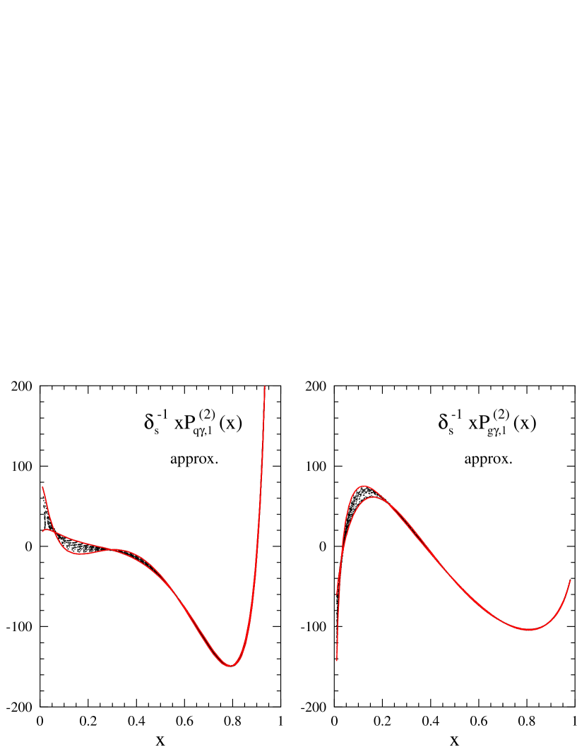
Figure 1: Approximations of the $N_{\rm f}^{0}$ parts $P_{\rm p\gamma,1}^{(2)}(x)$ of the NNLO photon-quark (p = q) and photon-gluon (p = g) splitting functions, as obtained from the six moments calculated in Sect. 3. The selected representatives (5.14) and (5.17) are shown by the full curves.

Figure 2: As Fig. 1, but for the $N_{\rm f}^{1}$ contributions $P_{\rm p\gamma,2}^{(2)}(x)$, with p = ns, ps (left) and p = g (right). The full curves represent the parametrizations in Eqs. (5.15), (5.16) and (5.18).

6 Numerical results in $x$-space

In this section we finally present the numerical impact of the NNLO corrections on the evolution of the photon’s parton distributions and on the structure function $F_{2}^{\,\gamma}$. Concerning the evolution kernels we confine ourselves to the respective inhomogeneous contributions $\mbox{\boldmath$P$}^{\gamma}$ and ${\cal I}_{2}^{\,\gamma}$ to Eqs. (4.2) and (4.21). The higher-order homogeneous (hadronic) non-singlet and singlet kernels have been discussed in detail in refs. [13, 39] and refs. [14], respectively; see also ref. [49] for a recent brief summary using the updated NNLO singlet splitting functions [15]. Also our subsequent illustrations of the solution of the evolution equations are restricted to the photon-specific inhomogeneous piece (4) and its contribution to $F_{2}^{\,\gamma}$. For brevity the results are shown only with all scales identified, i.e., at $\mu_{r}=\mu_{f}$ for the parton evolution and at $\mu_{r}\,(=\mu_{f})=Q$ for $F_{2}^{\,\gamma}$. The experimentally elusive longitudinal structure function $F_{L}^{\,\gamma}$ will not be addressed here.

In Figs. 3 and 4 the singlet photon-quark splitting functions $P_{\rm q\gamma}$ are displayed in the $\overline{\mbox{MS}}$ and the DIS_γ factorization schemes. The NLO and NNLO curves are shown for $\alpha_{\rm s}=0.2$ which corresponds to a scale between about 20 GeV² and 50 GeV², depending on the precise value of $\alpha_{\rm s}(M_{Z}^{2})$. After removing the charge factors $\delta_{\rm ns}$ and $\delta_{\rm s}$ defined in Eq. (2.29) only the NNLO terms depend on the number of flavours; the curves presented refer to $N_{\rm f}=4$. In the $\overline{\mbox{MS}}$ scheme (Fig. 3) the NNLO corrections are small except for small and very large values of $x$, amounting to less than $2\%\,$ for $0.1\leq x\leq 0.95$. Larger corrections for $x\!\rightarrow\!1$ are obvious since the NNLO splitting function $P^{(2)}\sim\ln^{4}(1\!-\!x)$ is more singular in this limit than its NLO analogue, $P^{(1)}\sim\ln^{2}(1\!-\!x)$. Likewise large NNLO effects are expected for small $x$ due to the first non-vanishing pure-singlet term $\sim 1/x$.

The higher-order corrections to $P_{\rm q\gamma}$ are somewhat larger in the DIS_γ scheme (Fig. 4) due to the absorption of the large coefficient function $C_{2,\gamma}$ (which, in particular, reverses the sign of the leading large-$x$ contribution). Here the NNLO corrections, under the conditions specified above, reach +6% at $x\simeq 0.6$ and exceed $-6\%$ for $x>0.9$. In the right parts of both figures the relative NNLO effects are also displayed (dotted curves) for the non-singlet splitting functions $P_{\rm ns\gamma}$, thus the pure-singlet effect can be directly read off from these figures. Also this effect is larger in the DIS_γ scheme where it exceeds 1% at $x<0.3$, instead of only at $x<0.15$ in the $\overline{\mbox{MS}}$ scheme.

The corresponding results for the photon-gluon splitting functions $xP_{\rm g\gamma}$ are shown in Fig. 5. The relative NNLO corrections (not shown separately for these quantities) are larger than in the photon-quark cases. However, the absolute size of $P_{\rm g\gamma}$ is much smaller than that of $P_{\rm q\gamma}$ except at small $x$. In the $\overline{\mbox{MS}}$ scheme $P_{\rm g\gamma}$ remains negative at $x\geq 0.2$ at NNLO. In the DIS_γ scheme, on the other hand, $P_{\rm g\gamma}$ is positive at large $x$, but seems to turn negative at NNLO for $x<0.05$.

Fig. 6 depicts, again for $\alpha_{\rm s}=0.2$ and $N_{\rm f}=4$, the inhomogeneous contribution $I_{2}^{\,\gamma}$ to the physical non-singlet evolution kernel (4.21). Here the NNLO corrections are particularly small, about 1% or less for $0.05\leq x<0.95$. As in Figs. 3 – 5, the present uncertainties arising from the residual error band for the ${\cal O}(a_{\rm em}a_{\rm s}^{2})$ photon-parton splitting functions are estimated by the NNLO_A and NNLO_B curves which derive from the upper and lower approximations, respectively, in Eqs. (5.14), (5.16) and (5.17) together with Eqs. (5.15) and (5.18). These uncertainties are virtually negligible at $x\geq 0.25$ and remain perfectly tolerable for $x\geq 0.05$, where they amount to less than $\pm 1\%$ for $P_{\rm q\gamma}$ and $I_{2}^{\,\gamma}$ with respect to the central results $\frac{1}{2}\,({\rm NNLO_{A}}+{\rm NNLO_{B}})$ not shown in the figures. This accuracy rapidly deteriorates towards small values of $x$.

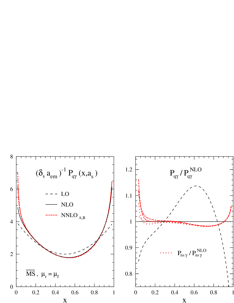
Figure 3: The perturbative expansion (4) of the photon-quark splitting function $P_{\rm q\gamma}(x,a_{\rm s})$ in the $\overline{\mbox{MS}}$ scheme for $\alpha_{\rm s}=0.2$ and $N_{\rm f}=4$. The relative NNLO corrections in the right part are also shown for the non-singlet splitting function $P_{\rm ns\gamma}$. Here and in the following three figures the subscripts ‘A’ and ‘B’ indicate the respective approximations in Eqs. (5.14), (5.16) and (5.18).

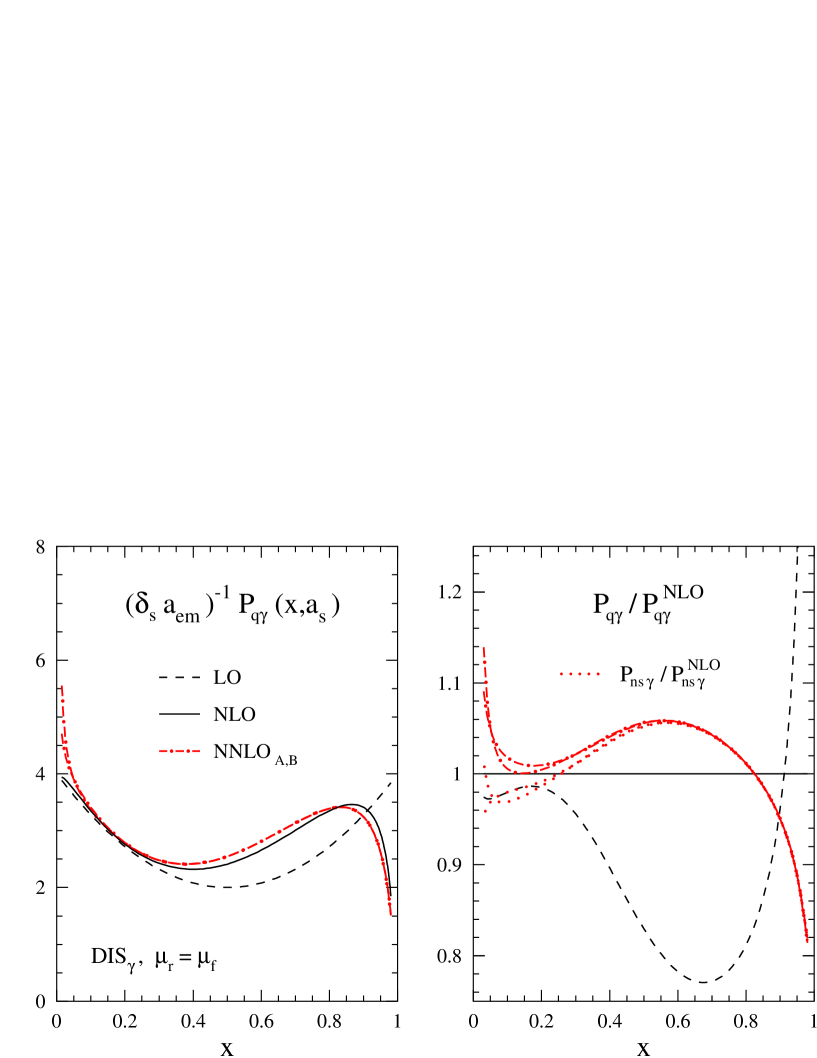
Figure 4: As Fig. 3, but for the photon-quark splitting functions (4) in the DIS_γ scheme.

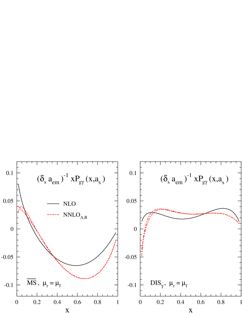
Figure 5: The NLO and NNLO approximations (4) for the photon-gluon splitting function $P_{\rm g\gamma}(x,a_{\rm s})$ in the $\overline{\mbox{MS}}$ scheme (left) and the DIS_γ scheme (right) for $\alpha_{\rm s}=0.2$ and $N_{\rm f}=4$. Note that $x\!\cdot\!P$ is displayed here, unlike in Fig. 3 and Fig. 4.

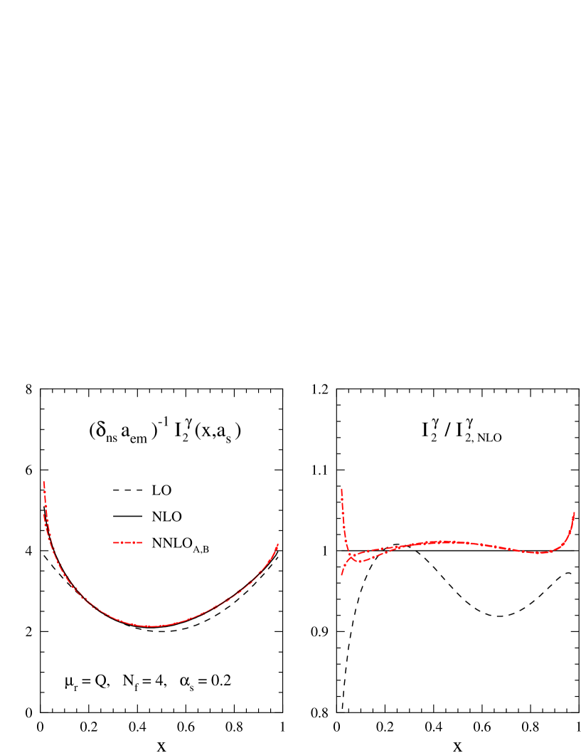
Figure 6: The perturbative expansion (4.22) of the inhomogeneous physical kernel $I_{2}^{\,\gamma}(x,a_{\rm s})$ for the evolution (4.21) of the structure function ${\cal F}_{2,\rm ns}^{\,\gamma}=1/x\>F_{2,\rm ns}^{\,\gamma}$ at the ‘default’ value of the scale $\mu_{r}$.

In Fig. 7 and Fig. 8 we present the inhomogeneous solutions $\alpha_{\rm em}^{-1}\,xf_{\rm inhom}^{\,\gamma}$, $f=\Sigma,\,g,$ for the singlet-quark and gluon distributions. The NLO approximation derived already in ref. [8] is obtained from the NNLO expression (4) by removing the third line, the $\mbox{\boldmath$U$}_{1}$ term in the second line and the $\mbox{\boldmath$U$}_{2}$ contribution to the first line; for the LO result also the rest of the second line and the $\mbox{\boldmath$U$}_{1}$ term in the first line have to be ignored. Like the NLO illustrations in refs. [7, 8] the results are shown at $\mu_{f}^{2}=50\mbox{ GeV}^{2}$ for $\mu_{f,0}^{2}=1\mbox{ GeV}^{2}$ and $N_{\rm f}=3$. For the strong coupling constants we use the realistic values $\alpha_{\rm s}(m_{f,0}^{2})\equiv 4\pi\,a_{0}=0.45$ at LO and 0.42 at NNLO and NNLO, and solve Eqs. (2.16) directly at $D=4$ with the appropriate number of terms in Eq. (2.17), i.e., including the coefficients $\beta_{k\leq m}$ [38] for the N^mLO evolution. Here and in Fig. 9 the (barely visible) differences of the NNLO_A and NNLO_B curves include the present uncertainties [39] of the hadronic NNLO splitting functions. The pattern of the NNLO corrections for the solutions roughly follows that of the corresponding splitting functions in Figs. 3 – 6. At this order $\mu_{f}^{2}=50\mbox{ GeV}^{2}$ is about the lowest scale where the inhomogeneous $\overline{\mbox{MS}}$ gluon density is positive over the full $x$-range.

Finally the structure functions $F_{2,\rm inhom}^{\,\gamma}(x,Q^{2}\!=\!50\mbox{ GeV}^{2})$ resulting from these parton densities (and their non-singlet analogues) are shown in Fig. 9 for the $\overline{\mbox{MS}}$ and the DIS_γ schemes. In both cases we have taken care to avoid spurious higher-order contributions which would arise from a simple convolution of Eq. (4) with the corresponding expansion of the hadronic coefficient functions, see Fig. 3 of ref. [50] for a NLO illustration. Note that the boundary conditions for $F_{2,\rm inhom}^{\,\gamma}$ are different in the two schemes: in the $\overline{\mbox{MS}}$ scheme this quantity is given by the corresponding photonic coefficient function (4.12) at $Q^{2}=\mu_{f,0}^{2}$, where it vanishes in the DIS_γ scheme according to Eq. (4.18). Thus, besides a ‘physical’ input describing the $F_{2}^{\,\gamma}$ at $Q^{2}=\mu_{f,0}^{2}$, a large additional ‘technical’ contribution to $\mbox{\boldmath$q$}^{\gamma}(\mu_{f,0}^{2})$ in Eq. (4.26) is required in the $\overline{\mbox{MS}}$ case. As mentioned above Eq. (4.21), the complete structure functions evolve approximately like non-singlet quantities at large $x$. In fact, under the conditions of Fig. 9, the complete DIS_γ result for $F_{2,\rm inhom}^{\,\gamma}$ and this non-singlet approximation differ by more than about 1% only at $x<0.2$, 0.25 and 0.3 at LO, NLO and NNLO, respectively.

Figure 7: The inhomogeneous LO, NLO and NNLO contributions to the photon’s singlet-quark and gluon distributions in the $\overline{\mbox{MS}}$ scheme at $\mu_{f}^{2}=50\mbox{ GeV}^{2}$, as obtained from Eq. (4) for $N_{\rm f}=3$ and $\mu_{f,0}^{2}=1\mbox{ GeV}^{2}$ with $\alpha_{\rm s}(\mu_{f,0}^{2})$ = 0.45 at LO and 0.42 at NLO and NNLO.

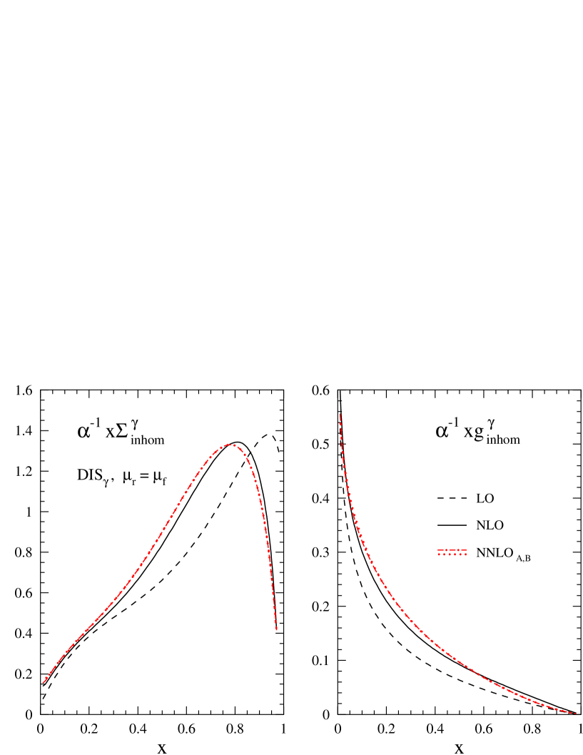
Figure 8: As Fig. 7, but for the inhomogeneous solutions in the DIS_γ factorization scheme (4).

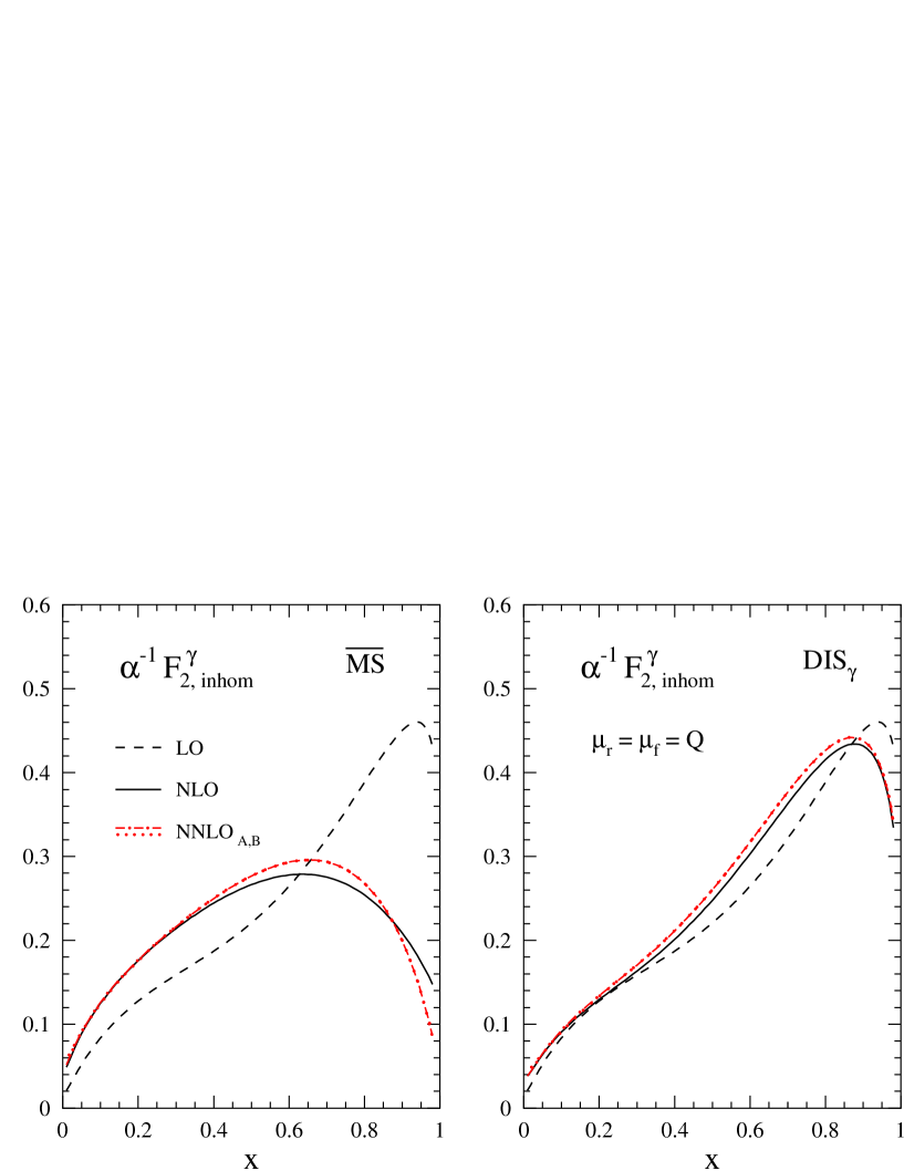
Figure 9: The perturbative expansion of the structure function $F_{2,\rm inhom}^{\,\gamma}$ at $Q^{2}=50\mbox{ GeV}^{2}$, as derived from the results shown in the previous two figures and their non-singlet counterparts by means of Eq. (4.10) in the $\overline{\mbox{MS}}$ scheme (left part) and Eq. (4.18) in the DIS_γ scheme (right part).

7 Conclusion

We have calculated the next-to-next-to-leading order QCD corrections to electron-photon DIS and to the evolution of the photon’s quark and gluon distributions. Our exact results for the corresponding photon-parton splitting functions are presently confined to the first six even-integer moments. Thus the practical applicability of the NNLO evolution is, for the time being, restricted to not too small values of the Bjorken variable $x$. This restriction seems to be more serious here than in lepton-hadron DIS, as the photon-parton splitting functions enter the evolution equations directly, not via smoothening convolutions with non-perturbative initial distributions. Consequently the effect of these functions is accurately known over a considerably smaller range of $x$ than that of their hadronic counterparts; a residual uncertainty of about $\pm 1\%$ or less is found for the total photon-quark splitting functions at NNLO only at $x\raisebox{-1.9919pt}{$\>\stackrel{{\scriptstyle>}}{{{\scriptstyle\sim}}}\>$}0.05$. However, only the perturbative component of the photon’s parton densities is affected by this uncertainty, and while this component dominates at large $x$, it represents only a small correction to the hadronic (homogeneous) contribution at small $x$. We thus expect that our results are sufficient for extending NLO analyses like those of refs. [51 – 54] to NNLO for the full $x$-range covered by the measurements at LEP.

Our present calculations are limited to effectively massless quarks, hence they do not apply to the charm and bottom contributions to the structure functions at small and intermediate scales. These contributions have been computed at NLO in refs. [55, 56]; corrected figures for $F_{2,\rm charm}^{\,\gamma}$ have been presented in ref. [57]. The NLO effects are found to be fairly small for this quantity, indicating that the NNLO corrections may be rather negligible [57]. While a full massive NNLO calculation does not seem feasible at present, these corrections could be estimated using the threshold resummation as done for the lepton-nucleon case in ref. [58].

By confining ourselves to the lowest order in the electromagnetic coupling we have assumed, as usual also in QCD analyses of lepton-hadron DIS, that the QED radiative corrections are treated elsewhere. The corresponding formalism has been set up in ref. [59] for measurements of the photon structure via the process $e^{+}e^{-}\!\rightarrow\!e^{+}e^{-}+X$. The non-factorizable corrections due to photon exchange between to two electron lines have been shown to be negligible in ref. [60], using a pseudoscalar as a simple model for the final state $X$. The dominant corrections arising from photon emissions of the ‘tagged’ electron line have been investigated for realistic measurements of the photon structure in refs. [61]. Neither of these studies has addressed the QED corrections to the subprocess $\gamma^{\ast}\gamma\!\rightarrow\!X$. We expect these corrections to be rather large, especially at the high scales which, hopefully, will become accessible to precise measurements in $e\gamma$ collisions at the future linear collider. Such contributions can be included in our present formalism by extending the analysis to higher order of electromagnetism. This extension is left to a future publication.

Fortran subroutines of our NNLO coefficient functions and of the approximations of the NNLO splitting functions can be found at http://www.nikhef.nl/$\sim$avogt.

Acknowledgments

We thank T. Gehrmann for providing the Fortran routine [47] for the harmonic polylogarithms. The work of S.M. has been supported by the German Federal Ministry for Research (BMBF) under grant BMBF-05HT9VKA and by the German Research Society (DFG) under contract No. FOR 264/2-1. The work of J.V. is part of the research program of the Dutch Foundation for Fundamental Research of Matter (FOM). The work of A.V. has been supported by the European Community TMR network ‘QCD and Particle Structure’ under contract No. FMRX–CT98–0194.

Appendix A

Here we present the analytic expressions for the anomalous dimensions and coefficient functions up to order $a_{\rm em}\,a_{\rm s}^{2}$ at the even-integer values $N=2,\,\ldots,\,12$. The notation is as in Sect. 3; in addition $C_{A}$ and $C_{F}$ are the standard QCD colour factors, $C_{A}\equiv N_{c}=3$ and $C_{F}=(N_{c}^{2}-1)/(2N_{c})=4/3$, and $\zeta_{i}$ stands for Riemann’s $\zeta$-function. The photon-quark anomalous dimensions are given by

$$(\delta_{\rm p}\,a_{\rm em})^{-1}\,k_{\rm p}^{N=2} = -\frac{4}{3}+a_{\rm s}C_{F}\left(-\frac{148}{27}\right)$$ (A.1)

$$\mbox{}+a_{\rm s}^{2}f_{\rm ps}C_{F}N_{\rm f}\left(-\frac{614}{243}\right)$$

$$\mbox{}+a_{\rm s}^{2}C_{F}C_{A}\left(-\frac{3022}{243}-\frac{32}{3}\zeta_{3}\right)$$

$$\mbox{}+a_{\rm s}^{2}C_{F}^{2}\left(-\frac{4310}{243}+\frac{64}{3}\zeta_{3}\right)$$

$$\mbox{}+a_{\rm s}^{2}C_{F}N_{\rm f}\left(\frac{268}{243}\right)$$

$$(\delta_{\rm p}\,a_{\rm em})^{-1}\,k_{\rm p}^{N=4} = -\frac{11}{15}+a_{\rm s}C_{F}\left(-\frac{56317}{9000}\right)$$ (A.2)

$$\mbox{}+a_{\rm s}^{2}f_{\rm ps}C_{F}N_{\rm f}\left(-\frac{3848699}{12150000}\right)$$

$$\mbox{}+a_{\rm s}^{2}C_{F}C_{A}\left(-\frac{101727401}{9720000}-\frac{261}{25}\zeta_{3}\right)$$

$$\mbox{}+a_{\rm s}^{2}C_{F}^{2}\left(-\frac{757117001}{24300000}+\frac{522}{25}\zeta_{3}\right)$$

$$\mbox{}+a_{\rm s}^{2}C_{F}N_{\rm f}\left(\frac{673127}{607500}\right)$$

$$(\delta_{\rm p}\,a_{\rm em})^{-1}\,k_{\rm p}^{N=6} = -\frac{11}{21}+a_{\rm s}C_{F}\left(-\frac{296083}{46305}\right)$$ (A.3)

$$\mbox{}+a_{\rm s}^{2}f_{\rm ps}C_{F}N_{\rm f}\left(-\frac{36356399}{326728080}\right)$$

$$\mbox{}+a_{\rm s}^{2}C_{F}C_{A}\left(-\frac{4774226099}{466754400}-\frac{1240}{147}\zeta_{3}\right)$$

$$\mbox{}+a_{\rm s}^{2}C_{F}^{2}\left(-\frac{2933980223981}{81682020000}+\frac{2480}{147}\zeta_{3}\right)$$

$$\mbox{}+a_{\rm s}^{2}C_{F}N_{\rm f}\left(\frac{1449736439}{1166886000}\right)$$

$$(\delta_{\rm p}\,a_{\rm em})^{-1}\,k_{\rm p}^{N=8} = -\frac{37}{90}+a_{\rm s}C_{F}\left(-\frac{51090517}{8164800}\right)$$ (A.4)

$$\mbox{}+a_{\rm s}^{2}f_{\rm ps}C_{F}N_{\rm f}\left(-\frac{986499379}{18895680000}\right)$$

$$\mbox{}+a_{\rm s}^{2}C_{F}C_{A}\left(-\frac{16806083022067}{1728324864000}-\frac{749}{108}\zeta_{3}\right)$$

$$\mbox{}+a_{\rm s}^{2}C_{F}^{2}\left(-\frac{4374484944665803}{113421319200000}+\frac{749}{54}\zeta_{3}\right)$$

$$\mbox{}+a_{\rm s}^{2}C_{F}N_{\rm f}\left(\frac{1373611188913}{1080203040000}\right)$$

$$(\delta_{\rm p}\,a_{\rm em})^{-1}\,k_{\rm p}^{N=10} = -\frac{56}{165}+a_{\rm s}C_{F}\left(-\frac{379479917}{62889750}\right)$$ (A.5)

$$\mbox{}+a_{\rm s}^{2}f_{\rm ps}C_{F}N_{\rm f}\left(-\frac{10520389912}{366894309375}\right)$$

$$\mbox{}+a_{\rm s}^{2}C_{F}C_{A}\left(-\frac{6245528269597}{684642974400}-\frac{17712}{3025}\zeta_{3}\right)$$

$$\mbox{}+a_{\rm s}^{2}C_{F}^{2}\left(-\frac{1091980048536213833}{27182465592975000}+\frac{35424}{3025}\zeta_{3}\right)$$

$$\mbox{}+a_{\rm s}^{2}C_{F}N_{\rm f}\left(\frac{29487804752071}{23534602245000}\right)$$

$$(\delta_{\rm p}\,a_{\rm em})^{-1}\,k_{\rm p}^{N=12} = -\frac{79}{273}+a_{\rm s}C_{F}\left(-\frac{9256843807}{1598647050}\right)$$ (A.6)

$$\mbox{}+a_{\rm s}^{2}f_{\rm ps}C_{F}N_{\rm f}\left(-\frac{60434951117}{3466052828784}\right)$$

$$\mbox{}+a_{\rm s}^{2}C_{F}C_{A}\left(-\frac{816463582581304612861}{95815031160008160000}-\frac{2563}{507}\zeta_{3}\right)$$

$$\mbox{}+a_{\rm s}^{2}C_{F}^{2}\left(-\frac{2960118366121154186145047}{71933134643376126120000}+\frac{5126}{507}\zeta_{3}\right)$$

$$\mbox{}+a_{\rm s}^{2}C_{F}N_{\rm f}\left(\frac{11634907579340558837}{9581503116000816000}\right)\>\>.$$

The photon-gluon anomalous dimensions read

$$(\delta_{\rm s}\,a_{\rm em})^{-1}\,k_{\rm g}^{N=2} = \,\,\,a_{\rm s}C_{F}\left(\frac{40}{27}\right)$$ (A.7)

$$\mbox{}+a_{\rm s}^{2}C_{F}C_{A}\left(-\frac{569}{243}+\frac{32}{3}\zeta_{3}\right)$$

$$\mbox{}+a_{\rm s}^{2}C_{F}^{2}\left(\frac{4796}{243}-\frac{64}{3}\zeta_{3}\right)$$

$$\mbox{}+a_{\rm s}^{2}C_{F}N_{\rm f}\left(\frac{940}{243}\right)$$

$$(\delta_{\rm s}\,a_{\rm em})^{-1}\,k_{\rm g}^{N=4} = \,\,\,a_{\rm s}C_{F}\left(\frac{2951}{4500}\right)$$ (A.8)

$$\mbox{}+a_{\rm s}^{2}C_{F}C_{A}\left(\frac{97099523}{24300000}+\frac{66}{25}\zeta_{3}\right)$$

$$\mbox{}+a_{\rm s}^{2}C_{F}^{2}\left(\frac{5594651}{1518750}-\frac{132}{25}\zeta_{3}\right)$$

$$\mbox{}+a_{\rm s}^{2}C_{F}N_{\rm f}\left(\frac{252613}{303750}\right)$$

$$(\delta_{\rm s}\,a_{\rm em})^{-1}\,k_{\rm g}^{N=6} = \,\,\,a_{\rm s}C_{F}\left(\frac{15418}{46305}\right)$$ (A.9)

$$\mbox{}+a_{\rm s}^{2}C_{F}C_{A}\left(\frac{25354637939}{8168202000}+\frac{176}{147}\zeta_{3}\right)$$

$$\mbox{}+a_{\rm s}^{2}C_{F}^{2}\left(\frac{29816260849}{20420505000}-\frac{352}{147}\zeta_{3}\right)$$

$$\mbox{}+a_{\rm s}^{2}C_{F}N_{\rm f}\left(\frac{76134169}{145860750}\right)$$

$$(\delta_{\rm s}\,a_{\rm em})^{-1}\,k_{\rm g}^{N=8} = \,\,\,a_{\rm s}C_{F}\left(\frac{32699}{163296}\right)$$ (A.10)

$$\mbox{}+a_{\rm s}^{2}C_{F}C_{A}\left(\frac{29969084304431}{12962436480000}+\frac{37}{54}\zeta_{3}\right)$$

$$\mbox{}+a_{\rm s}^{2}C_{F}^{2}\left(\frac{8625845880277}{11342131920000}-\frac{37}{27}\zeta_{3}\right)$$

$$\mbox{}+a_{\rm s}^{2}C_{F}N_{\rm f}\left(\frac{315324047}{843908625}\right)$$

$$(\delta_{\rm s}\,a_{\rm em})^{-1}\,k_{\rm g}^{N=10} = \,\,\,a_{\rm s}C_{F}\left(\frac{599864}{4492125}\right)$$ (A.11)

$$\mbox{}+a_{\rm s}^{2}C_{F}C_{A}\left(\frac{32269440044009551}{18121643728650000}+\frac{1344}{3025}\zeta_{3}\right)$$

$$\mbox{}+a_{\rm s}^{2}C_{F}^{2}\left(\frac{873823240941547}{1941604685212500}-\frac{2688}{3025}\zeta_{3}\right)$$

$$\mbox{}+a_{\rm s}^{2}C_{F}N_{\rm f}\left(\frac{119478173264}{420260754375}\right)$$

$$(\delta_{\rm s}\,a_{\rm em})^{-1}\,k_{\rm g}^{N=12} = \,\,\,a_{\rm s}C_{F}\left(\frac{1742495}{18270252}\right)$$ (A.12)

$$\mbox{}+a_{\rm s}^{2}C_{F}C_{A}\left(\frac{117808573254816607171}{83039693672007072000}+\frac{158}{507}\zeta_{3}\right)$$

$$\mbox{}+a_{\rm s}^{2}C_{F}^{2}\left(\frac{781495667102322375851}{2740309891176233376000}-\frac{316}{507}\zeta_{3}\right)$$

$$\mbox{}+a_{\rm s}^{2}C_{F}N_{\rm f}\left(\frac{5137635507236447}{22813102657144800}\right)\>\>.$$

The photonic coefficient functions for the structure function $F_{2}$ at $\mu_{r}=\mu_{f}=Q$ are given by

$$(\delta_{\rm p}\,a_{\rm em})^{-1}\,c_{2,\gamma}^{\,{\rm p},N=2} = -1+a_{\rm s}C_{F}\left(-\frac{4799}{405}+\frac{32}{5}\zeta_{3}\right)$$ (A.13)

$$\mbox{}+a_{\rm s}^{2}f_{\rm ps}C_{F}N_{\rm f}\left(-\frac{18007}{1458}+\frac{10144}{405}\zeta_{3}-\frac{64}{3}\zeta_{5}\right)$$

$$\mbox{}+a_{\rm s}^{2}C_{F}C_{A}\left(-\frac{440774}{3645}+\frac{26408}{405}\zeta_{3}-\frac{16}{3}\zeta_{4}+\frac{160}{3}\zeta_{5}\right)$$

$$\mbox{}+a_{\rm s}^{2}C_{F}^{2}\left(\frac{28403}{2430}+\frac{8296}{405}\zeta_{3}+\frac{32}{3}\zeta_{4}-\frac{320}{3}\zeta_{5}\right)$$

$$\mbox{}+a_{\rm s}^{2}C_{F}N_{\rm f}\left(\frac{65374}{3645}-\frac{3008}{405}\zeta_{3}\right)$$

$$(\delta_{\rm p}\,a_{\rm em})^{-1}\,c_{2,\gamma}^{\,{\rm p},N=4} = -\frac{133}{90}+a_{\rm s}C_{F}\left(-\frac{6410867}{360000}+\frac{36}{5}\zeta_{3}\right)$$ (A.14)

$$\mbox{}+a_{\rm s}^{2}f_{\rm ps}C_{F}N_{\rm f}\left(-\frac{207634473797}{4374000000}-\frac{2379889}{10125}\zeta_{3}+\frac{928}{3}\zeta_{5}\right)$$

$$\mbox{}+a_{\rm s}^{2}C_{F}C_{A}\left(-\frac{425129854859}{2449440000}+\frac{11978567}{141750}\zeta_{3}-\frac{261}{50}\zeta_{4}+\frac{164}{3}\zeta_{5}\right)$$

$$\mbox{}+a_{\rm s}^{2}C_{F}^{2}\left(-\frac{4566936087251}{61236000000}+\frac{18867971}{141750}\zeta_{3}+\frac{261}{25}\zeta_{4}-\frac{584}{3}\zeta_{5}\right)$$

$$\mbox{}+a_{\rm s}^{2}C_{F}N_{\rm f}\left(\frac{4247321033}{153090000}-\frac{123812}{14175}\zeta_{3}\right)$$

$$(\delta_{\rm p}\,a_{\rm em})^{-1}\,c_{2,\gamma}^{\,{\rm p},N=6} = -\frac{1777}{1260}+a_{\rm s}C_{F}\left(-\frac{12660217}{648270}+\frac{40}{7}\zeta_{3}\right)$$ (A.15)

$$\mbox{}+a_{\rm s}^{2}f_{\rm ps}C_{F}N_{\rm f}\left(-\frac{506384656389713}{3430644840000}-\frac{77458783}{138915}\zeta_{3}+\frac{16400}{21}\zeta_{5}\right)$$

$$\mbox{}+a_{\rm s}^{2}C_{F}C_{A}\left(-\frac{22283947715467}{117622108800}+\frac{68649953}{694575}\zeta_{3}-\frac{620}{147}\zeta_{4}+\frac{80}{3}\zeta_{5}\right)$$

$$\mbox{}+a_{\rm s}^{2}C_{F}^{2}\left(-\frac{986797608696253}{6861289680000}+\frac{65099719}{694575}\zeta_{3}+\frac{1240}{147}\zeta_{4}-\frac{880}{7}\zeta_{5}\right)$$

$$\mbox{}+a_{\rm s}^{2}C_{F}N_{\rm f}\left(\frac{3142023113107}{98018424000}-\frac{140188}{19845}\zeta_{3}\right)$$

$$(\delta_{\rm p}\,a_{\rm em})^{-1}\,c_{2,\gamma}^{\,{\rm p},N=8} = -\frac{16231}{12600}+a_{\rm s}C_{F}\left(-\frac{23994462871}{1175731200}+\frac{14}{3}\zeta_{3}\right)$$ (A.16)

$$\mbox{}+a_{\rm s}^{2}f_{\rm ps}C_{F}N_{\rm f}\left(-\frac{11841145531674938821}{32665339929600000}-\frac{3563866619}{3061800}\zeta_{3}+\frac{15232}{9}\zeta_{5}\right)$$

$$\mbox{}+a_{\rm s}^{2}C_{F}C_{A}\left(-\frac{28717038027651600293}{143727495690240000}+\frac{79435698877}{785862000}\zeta_{3}-\frac{749}{216}\zeta_{4}+\frac{118}{9}\zeta_{5}\right)$$

$$\mbox{}+a_{\rm s}^{2}C_{F}^{2}\left(-\frac{954577609184015777449}{5030462349158400000}+\frac{154197212633}{2357586000}\zeta_{3}+\frac{749}{108}\zeta_{4}-\frac{260}{3}\zeta_{5}\right)$$

$$\mbox{}+a_{\rm s}^{2}C_{F}N_{\rm f}\left(\frac{622760912995104859}{17965936961280000}-\frac{1122137}{200475}\zeta_{3}\right)$$

$$(\delta_{\rm p}\,a_{\rm em})^{-1}\,c_{2,\gamma}^{\,{\rm p},N=10} = -\frac{8704}{7425}+a_{\rm s}C_{F}\left(-\frac{72533010722807}{3486607740000}+\frac{216}{55}\zeta_{3}\right)$$ (A.17)

$$\mbox{}+a_{\rm s}^{2}f_{\rm ps}C_{F}N_{\rm f}\left(-\frac{209277550337208434702179}{287046836661816000000}-\frac{4286102504597}{1981027125}\zeta_{3}+\frac{35264}{11}\zeta_{5}\right)$$

$$\mbox{}+a_{\rm s}^{2}C_{F}C_{A}\left(-\frac{9568565675783568703229}{46259614172772000000}+\frac{366130385968}{3679050375}\zeta_{3}-\frac{8856}{3025}\zeta_{4}+\frac{200}{33}\zeta_{5}\right)$$

$$\mbox{}+a_{\rm s}^{2}C_{F}^{2}\left(-\frac{26284376777719892724358177}{117545679613013652000000}+\frac{3565449892804}{77260057875}\zeta_{3}+\frac{17712}{3025}\zeta_{4}-\frac{2096}{33}\zeta_{5}\right)$$

$$\mbox{}+a_{\rm s}^{2}C_{F}N_{\rm f}\left(\frac{462262990271149761829}{12721393897512300000}-\frac{302180374}{66891825}\zeta_{3}\right)$$

$$(\delta_{\rm p}\,a_{\rm em})^{-1}\,c_{2,\gamma}^{\,{\rm p},N=12} = -\frac{8110049}{7567560}+a_{\rm s}C_{F}\left(-\frac{6258789011950819}{299266727760000}+\frac{44}{13}\zeta_{3}\right)$$ (A.18)

$$\mbox{}+a_{\rm s}^{2}f_{\rm ps}C_{F}N_{\rm f}\left(-\frac{80246164545568080582270787397}{62342050024259309304000000}-\frac{3109586855303}{847767375}\zeta_{3}+\frac{499488}{91}\zeta_{5}\right)$$

$$\mbox{}+a_{\rm s}^{2}C_{F}C_{A}\left(-\frac{109517569276335628551465332167}{517918569432308108064000000}+\frac{59504875891511}{615479114250}\zeta_{3}-\frac{2563}{1014}\zeta_{4}+\frac{580}{273}\zeta_{5}\right)$$

$$\mbox{}+a_{\rm s}^{2}C_{F}^{2}\left(-\frac{194382513719914205037949320835327}{777654732002610624258096000000}+\frac{542538591728921}{16617936084750}\zeta_{3}+\frac{2563}{507}\zeta_{4}-\frac{4440}{91}\zeta_{5}\right)$$

$$\mbox{}+a_{\rm s}^{2}C_{F}N_{\rm f}\left(\frac{1937462197313198708954658827}{51791856943230810806400000}-\frac{294410659}{79053975}\zeta_{3}\right)\>\>,$$

and the corresponding results for $F_{L}$ read

$$(\delta_{\rm p}\,a_{\rm em})^{-1}\,c_{L,\gamma}^{\,{\rm p},N=2} = \frac{4}{3}+a_{\rm s}C_{F}\left(-\frac{232}{135}-\frac{32}{5}\zeta_{3}\right)$$ (A.19)

$$\mbox{}+a_{\rm s}^{2}f_{\rm ps}C_{F}N_{\rm f}\left(\frac{2686}{243}+\frac{3808}{15}\zeta_{3}-\frac{896}{3}\zeta_{5}\right)$$

$$\mbox{}+a_{\rm s}^{2}C_{F}C_{A}\left(-\frac{11788}{135}-\frac{6512}{45}\zeta_{3}+160\zeta_{5}\right)$$

$$\mbox{}+a_{\rm s}^{2}C_{F}^{2}\left(\frac{102566}{1215}+\frac{1856}{45}\zeta_{3}-\frac{320}{3}\zeta_{5}\right)$$

$$\mbox{}+a_{\rm s}^{2}C_{F}N_{\rm f}\left(\frac{2624}{405}+\frac{512}{45}\zeta_{3}\right)$$

$$(\delta_{\rm p}\,a_{\rm em})^{-1}\,c_{L,\gamma}^{\,{\rm p},N=4} = \frac{8}{15}+a_{\rm s}C_{F}\left(-\frac{5528}{1125}\right)$$ (A.20)

$$\mbox{}+a_{\rm s}^{2}f_{\rm ps}C_{F}N_{\rm f}\left(-\frac{48227851}{1215000}+\frac{4384}{135}\zeta_{3}\right)$$

$$\mbox{}+a_{\rm s}^{2}C_{F}C_{A}\left(-\frac{51480649}{354375}-\frac{174284}{4725}\zeta_{3}+128\zeta_{5}\right)$$

$$\mbox{}+a_{\rm s}^{2}C_{F}^{2}\left(\frac{912595079}{5670000}+\frac{451816}{4725}\zeta_{3}-256\zeta_{5}\right)$$

$$\mbox{}+a_{\rm s}^{2}C_{F}N_{\rm f}\left(\frac{520202}{39375}-\frac{64}{105}\zeta_{3}\right)$$

$$(\delta_{\rm p}\,a_{\rm em})^{-1}\,c_{L,\gamma}^{\,{\rm p},N=6} = \frac{2}{7}+a_{\rm s}C_{F}\left(-\frac{137761}{46305}\right)$$ (A.21)

$$\mbox{}+a_{\rm s}^{2}f_{\rm ps}C_{F}N_{\rm f}\left(\frac{97510126879}{4084101000}+\frac{61778}{315}\zeta_{3}-\frac{1760}{7}\zeta_{5}\right)$$

$$\mbox{}+a_{\rm s}^{2}C_{F}C_{A}\left(-\frac{43056771637}{437582250}-\frac{17446}{2205}\zeta_{3}+\frac{480}{7}\zeta_{5}\right)$$

$$\mbox{}+a_{\rm s}^{2}C_{F}^{2}\left(\frac{101548438631}{1021025250}+\frac{87148}{2205}\zeta_{3}-\frac{960}{7}\zeta_{5}\right)$$

$$\mbox{}+a_{\rm s}^{2}C_{F}N_{\rm f}\left(\frac{826872491}{87516450}-\frac{64}{63}\zeta_{3}\right)$$

$$(\delta_{\rm p}\,a_{\rm em})^{-1}\,c_{L,\gamma}^{\,{\rm p},N=8} = \frac{8}{45}+a_{\rm s}C_{F}\left(-\frac{51097}{25515}\right)$$ (A.22)

$$\mbox{}+a_{\rm s}^{2}f_{\rm ps}C_{F}N_{\rm f}\left(\frac{166525045327877}{1620304560000}+\frac{617672}{1575}\zeta_{3}-\frac{1664}{3}\zeta_{5}\right)$$

$$\mbox{}+a_{\rm s}^{2}C_{F}C_{A}\left(-\frac{103132581580249}{1485279180000}-\frac{393671}{779625}\zeta_{3}+\frac{128}{3}\zeta_{5}\right)$$

$$\mbox{}+a_{\rm s}^{2}C_{F}^{2}\left(\frac{2384408424295187}{35646700320000}+\frac{15446822}{779625}\zeta_{3}-\frac{256}{3}\zeta_{5}\right)$$

$$\mbox{}+a_{\rm s}^{2}C_{F}N_{\rm f}\left(\frac{36203618923}{5304568500}-\frac{1216}{1485}\zeta_{3}\right)$$

$$(\delta_{\rm p}\,a_{\rm em})^{-1}\,c_{L,\gamma}^{\,{\rm p},N=10} = \frac{4}{33}+a_{\rm s}C_{F}\left(-\frac{509195549}{352182600}\right)$$ (A.23)

$$\mbox{}+a_{\rm s}^{2}f_{\rm ps}C_{F}N_{\rm f}\left(\frac{551115536481640147}{2761393330080000}+\frac{694547002}{1091475}\zeta_{3}-\frac{10240}{11}\zeta_{5}\right)$$

$$\mbox{}+a_{\rm s}^{2}C_{F}C_{A}\left(-\frac{321273125948555419}{6230251067040000}+\frac{290422414}{156080925}\zeta_{3}+\frac{320}{11}\zeta_{5}\right)$$

$$\mbox{}+a_{\rm s}^{2}C_{F}^{2}\left(\frac{9053411269935853949}{188465094777960000}+\frac{1721766952}{156080925}\zeta_{3}-\frac{640}{11}\zeta_{5}\right)$$

$$\mbox{}+a_{\rm s}^{2}C_{F}N_{\rm f}\left(\frac{195749323625753}{38073756520800}-\frac{272}{429}\zeta_{3}\right)$$

$$(\delta_{\rm p}\,a_{\rm em})^{-1}\,c_{L,\gamma}^{\,{\rm p},N=12} = \frac{8}{91}+a_{\rm s}C_{F}\left(-\frac{197186301194}{179847793125}\right)$$ (A.24)

$$\mbox{}+a_{\rm s}^{2}f_{\rm ps}C_{F}N_{\rm f}\left(\frac{4911117022004232715153043}{15569942563501326000000}+\frac{463564050788}{496621125}\zeta_{3}-\frac{126208}{91}\zeta_{5}\right)$$

$$\mbox{}+a_{\rm s}^{2}C_{F}C_{A}\left(-\frac{47756006182490429534639}{1197687889500102000000}+\frac{5631384334}{2152024875}\zeta_{3}+\frac{1920}{91}\zeta_{5}\right)$$

$$\mbox{}+a_{\rm s}^{2}C_{F}^{2}\left(\frac{281711596115081884853551}{7784971281750663000000}+\frac{4695483724}{717341625}\zeta_{3}-\frac{3840}{91}\zeta_{5}\right)$$

$$\mbox{}+a_{\rm s}^{2}C_{F}N_{\rm f}\left(\frac{780777857066540089}{194429852191575000}-\frac{3392}{6825}\zeta_{3}\right)\>\>.$$

Appendix B

The exact expression for the ${\cal O}(a_{\rm em}a_{\rm s}^{2})$ contribution (5) to the transformation (4) of the photon-quark splitting function to the DIS_γ scheme is given by

$$\delta_{\rm p}^{-1}\Delta_{\rm DIS_{\gamma}}^{(2),\rm p}(x)\>=\>$$ (B.1)

$$16C_{F}^{2}\left\{-\left(56+\frac{2}{5}\frac{1}{x^{2}}+82x+50x^{2}+\frac{72}{5}x^{3}\right)H_{-1}\zeta_{2}-\left(\frac{431}{30}+\frac{4}{15}\frac{1}{x}+\frac{6}{5}x-\frac{102}{5}x^{2}\right)H_{2}\right.$$

$$\left.\mbox{}-\left(48+\frac{4}{15}\frac{1}{x^{2}}+\frac{308}{3}x+76x^{2}+\frac{48}{5}x^{3}\right)H_{-1,-1,0}-4(9+10x+16x^{2})H_{-2,-1,0}\right.$$

$$\left.\mbox{}-\left(21+\frac{2}{15}\frac{1}{x^{2}}-\frac{130}{3}x+34x^{2}-\frac{24}{5}x^{3}\right)H_{1}\zeta_{2}-\left(\frac{1883}{120}-\frac{4}{15}\frac{1}{x}-\frac{1683}{20}x+\frac{373}{5}x^{2}\right)H_{1}\right.$$

$$\left.\mbox{}-2\left(7-14x+6x^{2}\right)H_{1,1}\zeta_{2}-4\left(3-6x+7x^{2}\right)H_{3,1}-2\left(5-2x+6x^{2}\right)H_{2}\zeta_{2}\right.$$

$$\left.\mbox{}-2\left(5-10x-4x^{2}\right)H_{1}\zeta_{3}-4\left(2-2x+9x^{2}\right)H_{4}-\frac{1679}{180}-\frac{4}{45}\frac{1}{x}-\frac{4549}{120}x+\frac{276}{5}x^{2}\right.$$

$$\left.\mbox{}-\left(\frac{701}{72}-\frac{4}{45}\frac{1}{x}+\frac{129}{40}x+\frac{357}{5}x^{2}\right)H_{0}-8\left(1-2x+3x^{2}\right)H_{3,0}-4\left(2-4x+5x^{2}\right)H_{2,2}\right.$$

$$\left.\mbox{}-\left(\frac{809}{120}+\frac{4}{15}\frac{1}{x}+\frac{15521}{180}x+\frac{213}{5}x^{2}+\frac{32}{5}x^{3}\right)H_{0,0}-\left(\frac{5}{2}+3x+20x^{2}\right)H_{0,0,0,0}\right.$$

$$\left.\mbox{}-2\left(3-5x+2x^{2}\right)H_{2,0}-2\left(3-6x+10x^{2}\right)H_{1,3}-2\left(3-6x-2x^{2}\right)H_{1,0}\zeta_{2}\right.$$

$$\left.\mbox{}-\left(\frac{11}{2}+17x-60x^{2}\right)H_{2,1}-\left(\frac{9}{2}+\frac{47}{3}x+16x^{2}+\frac{48}{5}x^{3}\right)H_{3}-\left(\frac{9}{2}+11x-15x^{2}\right)H_{1,0}\right.$$

$$\left.\mbox{}-\left(3-8x+4x^{2}\right)H_{1,2}-2\left(1-2x+6x^{2}\right)H_{1,1,0,0}-\left(1-2x+12x^{2}\right)H_{2,0,0}\right.$$

$$\left.\mbox{}-\left(\frac{1}{2}+\frac{287}{6}x+36x^{2}+\frac{48}{5}x^{3}\right)H_{0,0,0}-\left(\frac{1}{2}+2x-8x^{2}\right)H_{1,0,0}+\left(\frac{6}{5}+\frac{4}{5}x+\frac{66}{5}x^{2}\right)\zeta_{2}^{2}\right.$$

$$\left.\mbox{}+\left(\frac{9}{2}+73x+16x^{2}+\frac{96}{5}x^{3}\right)H_{0}\zeta_{2}+\left(\frac{27}{4}-\frac{95}{2}x+30x^{2}\right)H_{1,1}+(8+36x^{2})H_{0,0}\zeta_{2}\right.$$

$$\left.\mbox{}+4\left(3+2x+8x^{2}\right)H_{-3,0}+2\left(1-2x-2x^{2}\right)H_{1,0,0,0}+\left(1-2x+16x^{2}\right)H_{2,1,1}\right.$$

$$\left.\mbox{}+2\left(3+6x+4x^{2}\right)(2H_{-1,0,0,0}+2H_{-1,3}+8H_{-1,-1}\zeta_{2}+8H_{-1,-1,-1,0}-4H_{-1,-2,0}\right.$$

$$\left.\mbox{}-4H_{-1,-1,2}-4H_{-1,0}\zeta_{2}-7H_{-1}\zeta_{3}-6H_{-1,-1,0,0})-2\left(19+14x+32x^{2}\right)H_{-2}\zeta_{2}\right.$$

$$\left.\mbox{}+8\left(2+x+8x^{2}\right)H_{0}\zeta_{3}+4\left(5+2x+8x^{2}\right)H_{-2,2}+4\left(7+6x+12x^{2}\right)H_{-2,0,0}\right.$$

$$\left.\mbox{}+\left(13+\frac{308}{3}x+62x^{2}+24x^{3}\right)\zeta_{3}+\left(\frac{431}{30}+\frac{8}{15}\frac{1}{x}+\frac{4328}{45}x-\frac{102}{5}x^{2}+\frac{32}{5}x^{3}\right)\zeta_{2}\right.$$

$$\left.\mbox{}+\left(\frac{31}{2}-74x+60x^{2}\right)H_{1,1,1}+\left(40+\frac{4}{15}\frac{1}{x^{2}}+\frac{200}{3}x+44x^{2}+\frac{48}{5}x^{3}\right)H_{-1,0,0}\right.$$

$$\left.\mbox{}+\left(32+\frac{4}{15}\frac{1}{x^{2}}+\frac{92}{3}x+12x^{2}+\frac{48}{5}x^{3}\right)H_{-1,2}+\left(16+\frac{172}{3}x+76x^{2}+\frac{48}{5}x^{3}\right)H_{-2,0}\right.$$

$$\left.\mbox{}+\Big{(}8H_{1,1,1,1}-2H_{1,1,0}-6H_{1,1,1,0}-10H_{1,1,2}-12H_{1,2,0}-14H_{1,2,1}-6H_{2,1,0}\Big{)}\,p_{\rm qg}(x)\right.$$

$$\left.\mbox{}+\left(\frac{613}{15}+\frac{8}{45}\frac{1}{x^{2}}+\frac{4}{15}\frac{1}{x}+\frac{4274}{45}x+\frac{288}{5}x^{2}+\frac{32}{5}x^{3}\right)H_{-1,0}\right\}$$

$$\mbox{}+16C_{A}C_{F}\left\{-\left(32+\frac{11}{45}\frac{1}{x^{2}}+\frac{394}{9}x+24x^{2}+\frac{44}{5}x^{3}\right)H_{-1,0}-\frac{233}{10}-\frac{11}{45}\frac{1}{x}+\frac{12283}{360}x-\frac{7}{10}x^{2}\right.$$

$$\left.-\left(\frac{15}{2}-27x+\frac{59}{3}x^{2}\right)H_{1,0,0}-\left(\frac{1825}{72}-\frac{467}{4}x+\frac{842}{9}x^{2}\right)H_{1}-\left(\frac{157}{6}+16x+96x^{2}\right)\zeta_{3}\right.$$

$$\left.-\left(\frac{167}{18}-\frac{464}{9}x+\frac{464}{9}x^{2}\right)H_{1,0}-\left(\frac{571}{72}-\frac{542}{9}x+\frac{248}{9}x^{2}-\frac{44}{5}x^{3}\right)H_{0,0}\right.$$

$$\left.-\left(\frac{701}{36}-\frac{466}{9}x+\frac{433}{9}x^{2}\right)H_{1,1}-\left(\frac{56}{3}+22x+\frac{158}{3}x^{2}\right)H_{-2,0}-2\left(2+5x+3x^{2}\right)H_{-1,2}\right.$$

$$\left.-\left(\frac{95}{6}-\frac{191}{6}x+\frac{433}{9}x^{2}\right)H_{2}-\left(\frac{40}{3}+\frac{122}{3}x+\frac{88}{3}x^{2}\right)H_{-1,0,0}-4\left(1+2x+3x^{2}\right)H_{-2,0,0}\right.$$

$$\left.-3\left(1+2x+4x^{2}\right)(3H_{0}\zeta_{3}+2H_{-3,0}+2H_{-2,2})-\left(\frac{1283}{120}-\frac{11}{45}\frac{1}{x}-\frac{21301}{360}x+\frac{3814}{45}x^{2}\right)H_{0}\right.$$

$$\left.-\left(\frac{11}{6}+\frac{85}{3}x+6x^{2}\right)H_{0}\zeta_{2}-\left(\frac{1}{10}-\frac{3}{5}x+\frac{22}{5}x^{2}\right)\zeta_{2}^{2}+\left(\frac{11}{12}+\frac{121}{6}x+\frac{29}{3}x^{2}\right)H_{0,0,0}\right.$$

$$\left.+\left(3-6x+8x^{2}\right)H_{2}\zeta_{2}+\left(5+10x+16x^{2}\right)H_{-2}\zeta_{2}+\left(6+12x+16x^{2}\right)H_{-2,-1,0}\right.$$

$$\left.+\left(\frac{11}{6}+\frac{19}{3}x+6x^{2}\right)H_{3}+\left(\frac{34}{3}-\frac{107}{3}x+\frac{79}{3}x^{2}\right)H_{1}\zeta_{2}+\left(\frac{46}{3}+\frac{137}{3}x+\frac{97}{3}x^{2}\right)H_{-1}\zeta_{2}\right.$$

$$\left.+\left(\frac{95}{6}-\frac{1361}{18}x+\frac{433}{9}x^{2}-\frac{44}{5}x^{3}\right)\zeta_{2}+\left(\frac{68}{3}+\frac{214}{3}x+\frac{158}{3}x^{2}\right)H_{-1,-1,0}-\frac{11}{3}x^{2}H_{2,1}\right.$$

$$\left.+\Big{(}7H_{-1}\zeta_{3}+4H_{-1,-2,0}-8H_{-1,-1}\zeta_{2}-8H_{-1,-1,-1,0}+6H_{-1,-1,0,0}+4H_{-1,-1,2}+4H_{-1,0}\zeta_{2}\right.$$

$$\left.-2H_{-1,0,0,0}-2H_{-1,3}\Big{)}\,p_{\rm qg}(-x)+4x\left(H_{0,0,0,0}+H_{4}-2H_{0,0}\zeta_{2}\right)+\bigg{(}H_{1}\zeta_{3}+4H_{1,0}\zeta_{2}\right.$$

$$\left.-2H_{1,0,0,0}+4H_{1,1}\zeta_{2}-2H_{1,1,0,0}-2H_{1,3}-2H_{2,0,0}-\frac{11}{3}H_{1,1,0}-\frac{11}{3}H_{2,0}-\frac{11}{6}H_{1,1,1}\bigg{)}\,p_{\rm qg}(x)\right\}$$

$$\mbox{}+\frac{16}{3}N_{F}C_{F}\left\{\left(1-2x\right)(H_{0}\zeta_{2}-H_{3})+\left(3-6x+2x^{2}\right)H_{1,0,0}-\left(\frac{1}{2}-x+2x^{2}\right)H_{0,0,0}\right.$$

$$\left.\mbox{}+\left(4+8x+4x^{2})(H_{-1,0,0}-H_{-1}\zeta_{2}-2H_{-1,-1,0}\right)-\left(4-8x+4x^{2}\right)H_{1}\zeta_{2}\right.$$

$$\left.\mbox{}+\left(\frac{41}{12}-\frac{44}{3}x+\frac{80}{3}x^{2}-\frac{24}{5}x^{3}\right)H_{0,0}-\left(7-\frac{55}{3}x+\frac{70}{3}x^{2}-\frac{24}{5}x^{3}\right)\zeta_{2}\right.$$

$$\left.\mbox{}+\left(\frac{83}{20}-\frac{2}{15}\frac{1}{x}-\frac{1091}{60}x+\frac{553}{15}x^{2}\right)H_{0}+\left(\frac{13}{3}-\frac{80}{3}x+\frac{80}{3}x^{2}\right)H_{1,0}\right.$$

$$\left.\mbox{}+\left(7-13x+\frac{70}{3}x^{2}\right)H_{2}+\frac{83}{10}+\frac{2}{15}\frac{1}{x}+\frac{7}{60}x-\frac{69}{5}x^{2}+\left(\frac{55}{6}-\frac{76}{3}x+\frac{70}{3}x^{2}\right)H_{1,1}\right.$$

$$\left.\mbox{}+\left(11-6x+18x^{2}\right)\zeta_{3}+2x^{2}H_{2,1}+\left(2H_{1,1,0}+H_{1,1,1}+2H_{2,0}\right)p_{\rm qg}(x)+8\left(1+x^{2}\right)H_{-2,0}\right.$$

$$\left.\mbox{}+\left(12+\frac{2}{15}\frac{1}{x^{2}}+\frac{16}{3}x+\frac{24}{5}x^{3}\right)H_{-1,0}+\left(\frac{137}{12}-\frac{105}{2}x+\frac{125}{3}x^{2}\right)H_{1}\right\}$$

$$\mbox{}+16f_{\rm ps}N_{F}C_{F}\left\{2(1-2x)\left(H_{4}-H_{0}\zeta_{3}-H_{0,0}\zeta_{2}+H_{0,0,0,0}-\frac{2}{5}\zeta_{2}^{2}\right)+\left(1-4x-\frac{16}{3}x^{2}\right)H_{0,0,0}\right.$$

$$\left.\mbox{}-\frac{175}{27}-\frac{20}{27}\frac{1}{x}+\frac{4327}{27}x-\frac{4132}{27}x^{2}-\left(3-\frac{40}{27}\frac{1}{x}-33x+\frac{850}{27}x^{2}\right)H_{1}\right.$$

$$\left.\mbox{}+\left(1+71x+\frac{1124}{27}x^{2}\right)H_{0}+\left(7+33x-\frac{44}{9}x^{2}\right)H_{0,0}-\left(4+11x+\frac{148}{9}x^{2}\right)(\zeta_{2}-H_{2})\right.$$

$$\left.\mbox{}-\left(1+8x-\frac{16}{3}x^{2}\right)(\zeta_{3}+H_{0}\zeta_{2}-H_{3})\right\}\>\>,$$

where the function $p_{\rm qg}(x)$ has been defined in Eq. (5.5). The corresponding result for the NNLO transformation of the photon-gluon splitting function, parametrized in Eq. (5.21), reads

$$\delta_{\rm s}^{-1}\Delta_{\rm DIS_{\gamma}}^{(2),\rm g}(x)\>=\>$$ (B.2)

$$32C_{F}^{2}\left\{\left(-\frac{67}{3}-\frac{4}{45}\frac{1}{x^{2}}-\frac{209}{9}x+\frac{4}{5}x^{3}\right)H_{-1,0}-\left(8+\frac{4}{3}x-\frac{8}{3}x^{2}\right)H_{-2,0}-\left(\frac{36}{5}+\frac{26}{5}x\right)\zeta_{2}^{2}\right.$$

$$\left.\mbox{}+\left(-\frac{85}{12}+\frac{13}{3}\frac{1}{x}+\frac{25}{12}x+\frac{2}{3}x^{2}\right)H_{1,1}-\left(5+\frac{22}{3}x\right)H_{0}\zeta_{2}+\left(\frac{1}{2}+\frac{29}{6}x-2x^{2}\right)H_{0,0,0}\right.$$

$$\left.\mbox{}+\left(-\frac{5}{2}-\frac{4}{3}\frac{1}{x}-\frac{13}{2}x+2x^{2}\right)\zeta_{3}+\left(-\frac{5}{2}+\frac{2}{3}\frac{1}{x}+\frac{5}{2}x-\frac{2}{3}x^{2}\right)H_{1,0,0}\right.$$

$$\left.\mbox{}+\left(-\frac{9}{4}-\frac{326}{9}x-\frac{2}{3}x^{2}+\frac{4}{5}x^{3}\right)\zeta_{2}+\left(\frac{1}{3}+\frac{11}{3}\frac{1}{x}-\frac{4}{3}x-\frac{8}{3}x^{2}\right)H_{1,0}-(7-x)\,H_{0}\zeta_{3}\right.$$

$$\left.\mbox{}+4(1-x)\left(H_{-2}\zeta_{2}+2H_{-2,-1,0}-H_{-2,0,0}+\frac{3}{4}H_{1}\zeta_{2}\right)+(1+x)\bigg{(}3H_{-1}\zeta_{2}-3H_{-1,0,0}\right.$$

$$\left.\mbox{}+6H_{-1,-1,0}+4H_{2}\zeta_{2}-3H_{0,0}\zeta_{2}-H_{2,0,0}-2H_{2,1,0}-7H_{2,1,1}-2H_{3,1}+\frac{5}{2}H_{0,0,0,0}+3H_{4}\bigg{)}\right.$$

$$\left.\mbox{}+\left(\frac{9}{4}+13x+\frac{2}{3}x^{2}\right)H_{2}+\left(\frac{41}{12}+\frac{13}{12}\frac{1}{x}+\frac{15}{2}x-12x^{2}\right)H_{1}+\left(6+5x+\frac{4}{3}x^{2}\right)H_{2,0}\right.$$

$$\left.\mbox{}+\left(\frac{39}{8}+\frac{2113}{72}x-\frac{8}{3}x^{2}-\frac{4}{5}x^{3}\right)H_{0,0}+(5+6x)H_{3}+\left(\frac{13}{2}+\frac{7}{2}x+\frac{14}{3}x^{2}\right)H_{2,1}\right.$$

$$\left.\mbox{}+\Big{(}H_{-1}\zeta_{2}-H_{-1,0,0}+2H_{-1,-1,0}\Big{)}p_{\rm g\gamma}(-x)+\left(H_{1}\zeta_{2}-H_{1,1,0}-\frac{7}{2}H_{1,1,1}\right)p_{g\gamma}(x)\right.$$

$$\left.\mbox{}+\left(\frac{3389}{360}+\frac{4}{45}\frac{1}{x}+\frac{311}{40}x-\frac{64}{5}x^{2}\right)H_{0}+\frac{2179}{180}+\frac{149}{180}\frac{1}{x}-\frac{77}{15}x-\frac{39}{5}x^{2}-8H_{-3,0}\right\}$$

$$\mbox{}+32C_{A}C_{F}\left\{-\left(\frac{20}{3}+\frac{2}{3}\frac{1}{x}+\frac{2}{3}x-\frac{16}{3}x^{2}\right)H_{-1,0}-\left(\frac{19}{3}-\frac{8}{3}\frac{1}{x}+\frac{25}{3}x+4x^{2}\right)H_{2,1}\right.$$

$$\left.\mbox{}-\left(\frac{11}{3}+\frac{14}{3}x+\frac{4}{3}x^{2}\right)H_{3}-\left(\frac{31}{9}-\frac{2}{3}\frac{1}{x}+\frac{128}{9}x-17x^{2}\right)H_{1}\right.$$

$$\left.\mbox{}-\left(\frac{8}{3}-\frac{4}{3}\frac{1}{x}+\frac{5}{3}x+\frac{8}{3}x^{2}\right)H_{2,0}-\left(\frac{37}{18}+\frac{67}{18}x+\frac{35}{9}x^{2}\right)H_{0,0}\right.$$

$$\left.\mbox{}-\left(1-5x-\frac{4}{3}x^{2}\right)H_{-2,0}+\left(\frac{1}{3}-\frac{8}{3}\frac{1}{x}+\frac{5}{3}x+\frac{2}{3}x^{2}\right)H_{1,1}+\left(\frac{7}{9}-\frac{2}{3}\frac{1}{x}-\frac{95}{9}x-\frac{56}{9}x^{2}\right)H_{2}\right.$$

$$\left.\mbox{}-\left(\frac{7}{9}-\frac{89}{9}x-\frac{56}{9}x^{2}\right)\zeta_{2}+\left(H_{-1,-1,0}-H_{-1,0,0}-H_{-1,2}+\frac{3}{2}H_{-1}\zeta_{2}\right)p_{\rm g\gamma}(-x)\right.$$

$$\left.\mbox{}+\left(H_{1,0,0}+2H_{1,1,0}+2H_{1,2}+3H_{1,1,1}-\frac{3}{2}H_{1}\zeta_{2}\right)p_{\rm g\gamma}(x)+\left(\frac{11}{3}+\frac{29}{3}x+\frac{4}{3}x^{2}\right)H_{0}\zeta_{2}\right.$$

$$\left.\mbox{}+(1-x)\,\Big{(}3H_{-2}\zeta_{2}-2H_{-3,0}+2H_{-2,-1,0}-2H_{-2,0,0}-2H_{-2,2}-H_{0}\zeta_{3}-2H_{0,0,0,0}\Big{)}\right.$$

$$\left.\mbox{}+(1+x)\,\Big{(}2H_{2,0,0}-3H_{2}\zeta_{2}+4H_{2,1,0}+6H_{2,1,1}+4H_{2,2}+4H_{3,0}+6H_{3,1}\Big{)}\right.$$

$$\left.\mbox{}+\left(\frac{21}{10}+\frac{27}{10}x\right)\zeta_{2}^{2}+\left(\frac{19}{6}+\frac{103}{6}x+2x^{2}\right)\zeta_{3}+\left(\frac{7}{2}-\frac{5}{3}\frac{1}{x}+\frac{1}{2}x-\frac{7}{3}x^{2}\right)H_{1,0}\right.$$

$$\left.\mbox{}+\left(\frac{97}{18}+\frac{67}{9}x-\frac{128}{9}x^{2}\right)H_{0}+\frac{317}{18}-\frac{1}{6}\frac{1}{x}-\frac{295}{6}x+\frac{571}{18}x^{2}+2x\,(H_{0,0,0}-H_{0,0}\zeta_{2}+2H_{4})\right\}$$

$$\mbox{}+\frac{32}{3}N_{F}C_{F}\left\{\left(\frac{11}{3}-\frac{26}{9}\frac{1}{x}+\frac{1}{3}x-\frac{10}{9}x^{2}\right)H_{1}-\frac{127}{9}+\frac{10}{9}\frac{1}{x}-\frac{35}{9}x+\frac{152}{9}x^{2}\right.$$

$$\left.\mbox{}-\left(3+21x+\frac{10}{9}x^{2}\right)H_{0}+\left(\frac{13}{3}+\frac{7}{3}x+\frac{8}{3}x^{2}\right)(\zeta_{2}-H_{2})-\left(\frac{16}{3}+\frac{22}{3}x+\frac{4}{3}x^{2}\right)H_{0,0}\right.$$

$$\left.\mbox{}+\Big{(}H_{1,0}+2H_{1,1}\Big{)}p_{\rm g\gamma}(x)+2(1+x)\,\Big{(}H_{3}-\zeta_{3}-H_{0}\zeta_{2}+H_{2,0}+2H_{2,1}\Big{)}\right\}\>\>.$$

Here we have used the abbreviation

$$p_{\rm g\gamma}(x)\>=\>\frac{4}{3x}+1-x-\frac{4}{3}x^{2}\>\>.$$

For the numerical evaluation of the harmonic polylogarithms up to weight four entering Eqs. (B.1) and (B.2) we have employed the program of ref. [47].

References

-
[1]
T.F. Walsh and P.M. Zerwas, Phys. Lett. B44 (1973) 195;
R.L. Kingsley, Nucl. Phys. B60 (1973) 45 - [2] E. Witten, Nucl. Phys. B120 (1977) 189
- [3] W.A. Bardeen and A.J. Buras, Phys. Rev. D20 (1979) 166; D21 (1980) 2041 (E)
- [4] N. Christ, B. Hasslacher, and A.H. Mueller, Phys. Rev. D6 (1972) 3543
- [5] R.J. De Witt, L.M. Jones, J.D. Sullivan, D.E. Willen and H.W. Wyld, Phys. Rev. D19 (1979) 2046; D20 (1979) 1751 (E)
- [6] M. Glück and E. Reya, Phys. Rev. D28 (1983) 2749
- [7] M. Fontannaz and E. Pilon, Phys. Rev. D45 (1992) 382; D46 (1992) 484 (E)
- [8] M. Glück, E. Reya, and A. Vogt, Phys. Rev. D45 (1992) 3986
- [9] E.B. Zijlstra and W.L. van Neerven, Phys. Lett. B272 (1991) 127; B273 (1991) 476; B297 (1992) 377; Nucl. Phys. B383 (1992) 525
- [10] S. Moch and J. A. M. Vermaseren, Nucl. Phys. B573 (2000) 853.
-
[11]
S.A. Larin, T. van Ritbergen, and J.A.M. Vermaseren, Nucl. Phys. B427 (1994) 41;
S.A. Larin, P. Nogueira, T. van Ritbergen, and J. Vermaseren, Nucl. Phys. B492 (1997) 338 - [12] A. Retey and J.A.M. Vermaseren, Nucl. Phys. B604 (2001) 281
- [13] W.L. van Neerven and A. Vogt, Nucl. Phys. B568, 263 (2000)
- [14] W.L. van Neerven and A. Vogt, Nucl. Phys. B588, 345 (2000)
- [15] W.L. van Neerven and A. Vogt, Phys. Lett. B490, 111 (2000)
-
[16]
M. Erdmann, The Partonic Structure of the Photon
(Springer Tracts in Mod. Phys. 138, 1997);
R. Nisius, Phys. Rept. 332 (2000) 165;
M. Krawczyk, A. Zembrzuski and M. Staszel, Phys. Rept. 345 (2001) 265 -
[17]
I.F. Ginzburg, G.L. Kotkin, V.G. Serbo and V.I. Telnov, Nucl. Instrum. Meth. 205 (1983) 47;
I.F. Ginzburg, G.L. Kotkin, S.L. Panfil, V.G. Serbo and V.I. Telnov, Nucl. Instrum. Meth. A219 (1984) 5;
V. I. Telnov, Nucl. Instrum. Meth. A294 (1990) 72 -
[18]
E. Accomando et al., Phys. Rept. 299 (1998) 1;
J.A. Aguilar-Saavedra et al., ECFA/DESY Linear Collider Physics Working Group Collab., hep-ph/0106315 - [19] A. Vogt, Nucl. Phys. (Proc. Suppl.) 82 (2000) 394
-
[20]
P. Aurenche, J. P. Guillet and M. Fontannaz, Phys. Lett. B338
(1994) 98;
P. Aurenche, L. Bourhis, M. Fontannaz and J. P. Guillet, Eur. Phys. J. C17 (2000) 413 -
[21]
M. Klasen and G. Kramer, Z. Phys. C76 (1997) 67;
M. Klasen, T. Kleinwort and G. Kramer, Eur. Phys. J. direct C1 (1998) 1 - [22] B. W. Harris and J. F. Owens, Phys. Rev. D56 (1997) 4007; D57 (1998) 5555
-
[23]
S. Frixione, Nucl. Phys. B507 (1997) 295;
S. Frixione and G. Ridolfi, Nucl. Phys. B507 (1997) 315 -
[24]
C. Anastasiou, E.W.N. Glover, C. Oleari and M.E.
Tejeda-Yeomans, Nucl. Phys. B601 (2001) 318; B601 (2001)
341; Nucl. Phys. B605 (2001) 486;
E.W.N. Glover, C. Oleari and M.E. Tejeda-Yeomans, Nucl. Phys. B605 (2001) 467-485 -
[25]
V.A. Smirnov, Phys. Lett. B460 (1999) 397;
J.B. Tausk, Phys. Lett. B469 (1999) 225 - [26] C. Anastasiou, E.W.N. Glover and M.E. Tejeda-Yeomans, in preparation
-
[27]
A.J. Buras, Rev. Mod. Phys. 52, 199 (1980);
E. Reya, Phys. Rept. 69 (1981) 195 -
[28]
G. ’t Hooft and M. Veltman, Nucl. Phys. B44 (1972) 189;
C.G. Bollini and J.J. Giambiagi, Nuovo Cim. 12B (1972) 20;
J.F. Ashmore, Lett. Nuovo Cim. 4 (1972) 289;
G.M. Cicuta and E. Montaldi, Lett. Nuovo Cim. 4 (1972) 329 - [29] W.A. Bardeen, A.J. Buras, D.W. Duke and T. Muta, Phys. Rev. D18 (1978) 3998
- [30] G. ’t Hooft, Nucl. Phys. B 61 (1973) 455
-
[31]
S.G. Gorishnii, S.A. Larin, and F.V. Tkachev, Phys. Lett. 124B
(1983) 217;
S.G. Gorishnii and S.A. Larin, Nucl. Phys. B283 (1987) 452 -
[32]
H. Kluberg-Stern and J.B. Zuber, Phys. Rev. D12 (1975) 467;
J.C. Collins, A. Duncan, and S.D. Joglekar, Phys. Rev. D16 (1977) 438 - [33] P. Nogueira, J. Comput. Phys. 105 (1993) 279
- [34] J.A.M. Vermaseren, Symbolic manipulation with FORM, (Computer Algebra Nederland, 1991); NIKHEF-00-032 (math-ph/0010025)
- [35] S.A. Larin, F.V. Tkachev, and J.A.M. Vermaseren, NIKHEF-H-91-18.
- [36] M. Glück, E. Reya and A. Vogt, Phys. Rev. D48 (1993) 116; D51 (1993) 1427 (E)
- [37] J. Chyla, JHEP 0004 (2000) 007
-
[38]
O.V. Tarasov, A.A. Vladimirov, and A.Yu. Zharkov, Phys. Lett. B93 (1980) 429;
S.A. Larin and J.A.M. Vermaseren, Phys. Lett. B303 (1993) 334 - [39] W.L. van Neerven and A. Vogt, Nucl. Phys. B603 (2001) 42
- [40] W. Furmanski and R. Petronzio, Z. Phys. C11 (1982) 293
- [41] R.K. Ellis, Z. Kunszt and E.M. Levin, Nucl. Phys. B420 (1994) 517; B433 (1994) 498 (E)
- [42] J. Blümlein and A. Vogt, Phys. Rev. D58 (1998) 014020
-
[43]
G. Rossi, Phys. Rev. D29 (1984) 852;
M. Drees, Z. Phys. C27 (1985) 123 - [44] E. Remiddi and J.A.M. Vermaseren, Int. J. Mod. Phys. A15 (2000) 725
-
[45]
J. A. M. Vermaseren, Int. J. Mod. Phys. A14 (1999) 2037;
J. Blümlein and S. Kurth, Phys. Rev. D60 (1999) 014018 - [46] L. Lewin, Polylogarithms and Associated Functions (North-Holland, 1981)
- [47] T. Gehrmann and E. Remiddi, Comput. Phys. Commun. 141 (2001) 296
- [48] W. Furmanski and R. Petronzio, Phys. Lett. B97 (1980) 437
- [49] W.L. van Neerven and A. Vogt, hep-ph/0107194
- [50] A. Vogt, Proceedings of the Workshop on Two–Photon Physics at LEP and HERA, Lund, May 1994, eds. G. Jarlskog and L. Jönsson (Lund Univ., 1994), p. 141 (hep-ph/9407320)
- [51] M. Glück, E. Reya, and A. Vogt, Phys. Rev. D46 (1992) 1973
- [52] L. E. Gordon and J.K. Storrow, Z. Phys. C56 (1992) 307; Nucl. Phys. B489 (1997) 405
- [53] P. Aurenche, J.P. Guillet, and M. Fontannaz, Z. Phys. C64 (1994) 621
- [54] M. Glück, E. Reya, and I. Schienbein, Phys. Rev. D60 (1999) 054019
- [55] E. Laenen, S. Riemersma, J. Smith, and W.L. van Neerven, Nucl. Phys. B392 (1993) 162
- [56] E. Laenen, S. Riemersma, J. Smith, and W.L. van Neerven, Phys. Rev. D49 (1994) 5753
- [57] E. Laenen and S. Riemersma, Proceedings of Photon ’95, Sheffield, UK, April 1995, eds. D.J. Miller, S.L. Cartwright and V. Khoze (World Scientific 1995), p. 117 (hep-ph/9505230)
- [58] E. Laenen and S. Moch, Phys. Rev. D59 (1999) 034027
- [59] W.L. van Neerven and J.A.M. Vermaseren, Nucl. Phys. B238 (1984) 73
- [60] W.L. van Neerven and J.A.M. Vermaseren, Phys. Lett. B142 (1984) 80
- [61] E. Laenen and G.A. Schuler, Phys. Lett. B374 (1996) 217; Proceedings of Photon ’97, Egmond aan Zee, Netherlands, May 1997, eds. A. Buijs and F.C. Erné (World Scientific 1997), p. 57 (hep-ph/9708261)