DESY 01–172

TSL/ISV–2001–0254

October 2001

Diffusion into infra-red and unitarization
of the BFKL pomeron
K.  Golec–Biernat^(a,d), L.  Motyka^(b,e) and A. M.  Staśto^(c,d)

^(a)II. Institut für Theoretische Physik, Universität Hamburg, Germany
^(b) High Energy Physics, Uppsala University, Box 535, 751-21 Uppsala, Sweden

^(c) INFN Sezione di Firenze, Via G. Sansone 1, 50019 Sesto Fiorentino (FI), Italy

^(d)H. Niewodniczański Institute of Nuclear Physics, Radzikowskiego 152, Kraków, Poland

^(e)Institute of Physics, Jagiellonian University, Reymonta 4, Kraków, Poland

The BFKL pomeron in perturbative QCD is plagued by the lack of unitarity and diffusion into the infra-red region of gluon virtualities. These two problems are intimately related. We perform numerical studies of the evolution equation proposed by Balitsky and Kovchegov which unitarizes the BFKL pomeron. We show how diffusion into the infra-red region is suppressed due to the emergence of a saturation scale and scaling behaviour. We study universality of this phenomenon as well as its dependence on subleading corrections to the BFKL pomeron such as the running coupling and kinematic constraint. These corrections are very important for phenomenological applications.

1 Introduction

The Balitsky-Fadin-Kuraev-Lipatov (BFKL) equation [1] describes the behaviour of scattering amplitudes in the limit of high center-of-mass energy $\sqrt{s}$, in the kinematic range where perturbative QCD is applicable. In the leading logarithmic approximation (LLA), $\alpha_{s}\ll 1$ and $\alpha_{s}\log s\sim 1$, the behaviour is determined by the leading singularity in the complex angular momentum plane at $j=1+4N_{c}\alpha_{s}\ln 2/\pi$, which corresponds to the vacuum quantum number exchange. In the context of QCD such exchange is called the BFKL pomeron. For $s\rightarrow\infty$, the corresponding total cross section rises with energy, $\sigma^{tot}\sim s^{\/j-1}=s^{\/0.5}$ for $\alpha_{s}\approx 0.2$, violating the Froissart bound reflecting the fundamental principle of unitarity of the $S$-matrix: $\sigma^{tot}\leq C\log(s)$. The next-to-leading corrections to the BFKL equation [2] reduce the rise of the total cross section but the power-like form in $s$ still holds.

Another cumbersome property of the BFKL equation is the diffusion of gluon virtualities (dominated by the transverse momentum) into the infra-red region. The BFKL pomeron is made up of two interacting reggeized gluons, diagrammatically represented by a set of gluon ladders. With increasing energy, the distribution of the gluon virtualities along the ladder quickly enters the low momentum region around $\Lambda_{\rm QCD}$ with the characteristic diffusion pattern. Thus the description which is rooted in perturbative QCD is not consistent in the high energy limit.

The intuitive physical picture of new phenomena, called screening or saturation effects, which are in agreement with the unitarity bound at high energy was provided in [3]. In the context of the BFKL diffusion the picture looks as follows. The transverse size of gluons with transverse momentum $k_{\perp}$ is proportional to $1/k_{\perp}^{2}$. For large $k_{\perp}$, the BFKL mechanism of gluon radiation, $g\rightarrow gg$, populates the transverse space with large number of small size gluons per unit of rapidity $Y\sim\ln s$. The same mechanism also applies to large size gluons with small transverse momenta. In this case, however, the BFKL approach is incomplete since the gluons strongly overlap and fusion processes, $gg\rightarrow g$, are equally important. After taking these processes into account, unitarity is restored by taming the rise of the gluon density with transverse momenta below some energy-dependent scale $Q_{s}(Y)$, called saturation scale. The emergence of such scale is a fundamental property of the parton saturation phenomenon. The saturation scale rises monotonically with $s$, and for large enough rapidity $Y$ for which $Q_{s}(Y)\gg\Lambda_{QCD}$, the presented approach to the high energy scattering remains consistent. In this sense the solution to the unitarity problem cures in turn the infra-red diffusion problem.

The parton saturation idea is realized with the help of non-linear evolution equations in which the gluon splitting is described by a linear term while a negative non-linear term results from the competing gluon recombination. The first equation of this type for the gluon density was postulated in [3] in the double logarithmic approximation. More rigorous derivation was given in [4]. The attempts to go beyond the double-log asymptotics resulted in formulations based on semi-classical QCD methods [5, 6] since the region of parton saturation is characterized by large values of colour fields. A different approach to unitary generalization of the BFKL equation was proposed by Balitsky [7, 8, 9]. By using the operator product expansion for high energy scattering in QCD, he derived an infinite hierarchy of coupled equations for $n$-point Wilson-line operators. Weigert managed to simplify the form of these equations by writing them as a functional evolution equation for the generating functional of the Wilson-line operators [10]. The connection between the effective theory for the Colour Glass Condensate [5, 6] and the evolution equation found by Weigert has been established in [11]. Another derivation of the small-$x$ non-linear equation has been recently given in [12].

The Balitsky’s equations decouple in the large $N_{c}$ limit. In this limit, the equation for the 2-point function was independently derived by Kovchegov [13] in the dipole picture [14]. The equation unitarizes the BFKL equation by including a quadratic term determined by the three-pomeron vertex [15]. The properties of this equation were investigated in [16]-[23] supporting the picture of parton saturation. The equation introduces the saturation scale below which the non-linear effects lead to saturation of the gluon density. Recently, an extended version of these equations which include cubic terms has been derived [24].

In this paper we concentrate on numerical studies of the Balitsky-Kovchegov evolution equation [13]. We illustrate the emergence of the saturation region with the saturation scale and scaling behaviour of the resulting cross sections. Such scaling was found in the DIS data at small $x$ [25], after being inspired by the saturation model [26]. We contrast the properties of the non-linear BK equation with those resulting from the linear BFKL equation. In particular, we show the effect of unitarization on infra-red diffusion. These results serve as the starting point for the analysis of the Balitsky-Kovchegov equation with subleading corrections given by the running QCD coupling and kinematic constraint. Although subleading, these corrections are very important for phenomenological applications and we carefully examine their impact onto the universality of the parton saturation phenomenon.

2 The Balitsky-Kovchegov equation

The Balitsky-Kovchegov (BK) equation was derived for the deep inelastic scattering of virtual photon on a large nucleus by the resummation of multiple pomeron exchanges in the leading logarithmic approximation (when $\alpha_{s}\ll 1$, $\alpha_{s}\ln(1/x)\sim 1$ and $x\simeq Q^{2}/s$) and in the large $N_{c}$ limit [13, 16].

The physical picture of this process is provided in the rest frame of the nucleus. In the small $x$ limit, the virtual photon splits into a $q\bar{q}$ pair long before the interaction with the nucleus. Then the $q\bar{q}$ pair interacts with the nucleus. In this case the nucleus structure function is given by

$$F_{2}(x,Q^{2})\,=\,\frac{Q^{2}}{4\pi^{2}\alpha_{em}}\int d^{\/2}{\bf r}\,dz\left\{|\Psi_{T}(z,{\bf r},Q^{2})|^{2}+|\Psi_{L}(z,{\bf r},Q^{2})|^{2}\right\}\,\hat{\sigma}(x,{\bf r})$$ (1)

where $\Psi_{T,L}$ are the light-cone wave functions for the transversely and longitudinally polarized virtual photon, and $\hat{\sigma}$ is the dipole cross section describing the interaction of the $q\bar{q}$ dipole with the nucleus. Here, ${\bf r}={\bf r}_{1}-{\bf r}_{0}$ is the transverse size of the dipole (${\bf r}_{1},{\bf r}_{0}$ are the transverse coordinates of the quark and antiquark) and $z$ is the longitudinal fraction of the photon’s momentum carried by the quark. The sum of the squares of the photon wave functions (for massless quarks) is given by

$$|\Psi_{T}|^{2}+|\Psi_{L}|^{2}=\frac{N_{c}\/\alpha_{em}}{2\pi^{2}}\,\sum_{f}e_{f}^{2}\left\{[z^{2}+(1-z)^{2}]\,\epsilon^{2}\,K_{1}^{2}(\epsilon r)+4\,Q^{2}z^{2}(1-z)^{2}\,K_{0}^{2}(\epsilon r)\right\}$$ (2)

where $\epsilon^{2}=z(1-z)\,Q^{2}$, $K_{0,1}$ are the Bessel–Mc Donald functions and the sum is performed over all active quark flavours $f$. The dipole cross section is related to the imaginary part of the forward scattering amplitude of the $q\bar{q}$ dipole on the nucleus $N({\bf r},{\bf b},Y)$,

$$\hat{\sigma}(x,{\bf r})\,=\,2\!\int d^{\/2}{{\bf b}}\,N({\bf r},{\bf b},Y),$$ (3)

where ${\bf b}=({\bf r}_{1}+{\bf r}_{0})/2$ is the impact parameter of the $q\bar{q}$ dipole.

The BK equation is an evolution equation for the amplitude $N({\bf r},{\bf b},Y)$. In the derivation [13] it was assumed that the $q\bar{q}$ pair develops a cascade of gluons which, in the large $N_{c}$ limit, form a system of $3$-$\bar{3}$ dipoles. Each dipole interacts independently with nucleons in the nucleus via two-gluon exchange. In this way the following non-linear evolution equation was found

$$\frac{\partial N({\bf r},{\bf b},Y)}{\partial Y} = \overline{\alpha}_{s}\ (K\otimes N)({\bf r},{\bf b},Y)$$ (4)

$$- \overline{\alpha}_{s}\,\int\frac{d^{2}{\bf r}^{\prime}}{2\pi}\,\frac{r^{2}}{r^{\/\prime 2}({\bf r}+{\bf r}^{\prime})^{2}}\,N({\bf r}+{\bf r}^{\prime},{\bf b}+\frac{{\bf r}^{\prime}}{2},Y)\;N({\bf r}^{\prime},{\bf b}+\frac{{\bf r}+{\bf r}^{\prime}}{2},Y).$$

where $\overline{\alpha}_{s}=N_{c}\alpha_{s}/\pi$, and the linear term is determined by the BFKL kernel

$$\\ (K\otimes N)({\bf r},{\bf b},Y)=\int\frac{d^{2}{\bf r}^{\prime}}{\pi\/r^{\/\prime 2}}\,\left\{\frac{r^{2}}{({\bf r}+{\bf r}^{\prime})^{2}}\,N({\bf r}+{\bf r}^{\prime},{\bf b},Y)-\frac{r^{2}}{r^{\/\prime 2}+({\bf r}+{\bf r}^{\prime})^{2}}\,N({\bf r},{\bf b},Y)\right\}.\\$$ (5)

Thus in the linear approximation, when each dipole scatters only once off the nucleus, the BFKL equation in the dipole picture is obtained. The non-linear term in (4) takes into account multiple scatterings and is essentially determined by the triple pomeron vertex [15] in the large $N_{c}$ limit. Eq. (4) unitarizes the BFKL pomeron in the sense that at $x\rightarrow 0$ and $Q^{2}$ fixed,

$$F_{2}\,\sim\,Q^{2}\,\ln(1/x)\,.$$ (6)

Thus the power-like rise with energy for the BFKL pomeron is tamed [16].

In the infinite momentum frame, the BK equation resums fan diagrams with the BFKL ladders, corresponding to the pomeron, splitting into two ladders. This type of summation was originally proposed by Gribov, Levin and Ryskin (GLR) [3] in the double logarithmic approximation (DLA): $\alpha_{s}\ll 1$ and $\alpha_{s}\ln(1/x)\ln(Q^{2}/\Lambda_{QCD}^{2})\sim 1$. It was shown in [13] that eq. (4) reduces to the GLR equation for the integrated gluon distribution.

The BK equation was derived for a large nucleus by the summation of the leading contributions in powers of the atomic number of the nucleus $A$. Other contributions, e.g. those corresponding to loops built out of the BFKL ladders, are suppressed by powers of $A$. However, this equation can be applied to a nucleon as a model which hints towards the most important contributions to the structure function at small $x$. The success of the saturation model [26] in the description of the small-$x$ DIS data is an indication that this equation might also properly identify the leading contribution for a nucleon.

Figure 1: Kinematics of the gluons in the BFKL ladder. $x$ and $x/z$ are the longitudinal momentum fractions, and $k$, $k^{\prime}$ and $q=k-k^{\prime}$ are transverse momenta of the gluons.

A substantial complication of the analysis of eq. (4) is related to the coupling between the ${\bf r}$ and ${\bf b}$ variables. In our presentation we follow the approximation made in the earlier analyses that the dominant contribution to $F_{2}$ is given by the tranverse sizes $r$ for which $r\ll b<R$, where $R$ is the nucleus size. In this case the coupling between $r$ and $b$ can be neglected and eq. (4) becomes independent of $b$. Thus, the $b$-dependence can be suppressed in $N({\bf r},{\bf b},Y)$. It can then enter only through the initial condition for the evolution equation. In a more refined analysis, however, the exact $b$-dependence should be taken into account.

For an azimuthally symmetric solution, $N({\bf r},Y)=N(r,Y)$, eq. (4) can be rewritten in momentum space in a much simpler form after performing the Fourier transform [16]

$$\phi(k,Y)\,=\,\int\frac{d^{2}{\bf r}}{2\pi}\exp(-i{\bf k}\cdot{\bf r})\,\frac{N(r,Y)}{r^{2}}\,=\,\int_{0}^{\infty}\frac{dr}{r}\,J_{0}(k\/r)\,N(r,Y),$$ (7)

where $J_{0}$ is the Bessel function. In this case the following equation is obtained

$$\frac{\partial\phi(k,Y)}{\partial Y}\,=\,\overline{\alpha}_{s}\,(K^{\prime}\otimes\phi)(k,Y)\,-\ \overline{\alpha}_{s}\,\phi^{\,2}(k,Y),$$ (8)

and the action of the BFKL kernel (appropriately shifted in the space of the Mellin moments in $k^{2}$) is given by

$$(K^{\prime}\otimes\phi)(k,Y)\,=\,\int_{0}^{\infty}\frac{dk^{\prime 2}}{k^{\prime 2}}\,\left\{\frac{k^{\prime 2}\,\phi(k^{\prime},Y)\,-\,k^{2}\,\phi(k,Y)}{|k^{2}\,-\,k^{\prime 2}|}\,+\,\frac{k^{2}\,\phi(k,Y)}{\sqrt{4k^{\prime 4}\,+\,k^{4}}}\right\},$$ (9)

where now $k$ and $k^{\prime}$ are the transverse momenta of the exchanged gluons in the BFKL ladder, see Fig. 1. The form (8) of the BK equation serves as the starting point of our analysis.

3 Saturation scale and scaling

In this section we present some interesting properties of the solutions of the Balitsky-Kovchegov equation, based on a numerical analysis of eq. (8). In particular, we illustrate how the BFKL diffusion is suppressed due to non-linear effects leading to emergence of a saturation scale. This issue was also studied in Refs. [17]-[22].

When studying diffusion in transverse momenta, it is convenient to illustrate the results in terms of the function $\phi(k,Y)$ multiplied by $k$. The reason is very simple. In the linear case, when the non-linear term in eq. (8) is neglected, the resulting BFKL equation has the asymptotic solution which is proportional to $k^{-1}$. The remaining term exhibits the well know diffusion pattern in the variable $\eta=\ln(k/k_{0})$. Thus for

$$k\,\phi(k,Y)\,=\,\exp({\overline{\alpha}}_{s}\chi(0)Y)\,\frac{1}{\sqrt{\pi{\overline{\alpha}}_{s}\chi^{\prime\prime}(0)Y}}\,\exp\left(-\,\frac{\ln^{2}(k^{2}/k_{0}^{2})}{2{\overline{\alpha}}_{s}\chi^{\prime\prime}(0)Y}\right),$$ (10)

where $\chi(0)=4\ln 2$ and $\chi^{\prime\prime}(0)=28\,\zeta(3)$, diffusion is clearly isolated. We will contrast the behaviour (10) with the solution of the non-linear BK equation.

In order to solve eq. (8) an initial condition at $Y=0$ has to be specified. We start from the condition which is concentrated at some value $\eta_{1}$ in the logarithmic variable $\eta$

$$k\,\phi(k,Y=0)\,=\,\delta(\eta-\eta_{1}).$$ (11)

In Fig. 2 we show the solutions for different values of $Y$ for the linear (BFKL) and the non-linear (BK) equation. The BFKL solutions illustrate the features of eq. (10), i.e the unlimited rise with rapidity (energy) and diffusion into the domain of large and small values of the transverse momentum $k$. For the solutions of the BK equation, however, the small $k$ domain is strongly suppressed and the rise with energy is significantly bounded. For large values of $k$, when the non-linearity in the BK equation is small, the BK and BFKL solutions coincide.

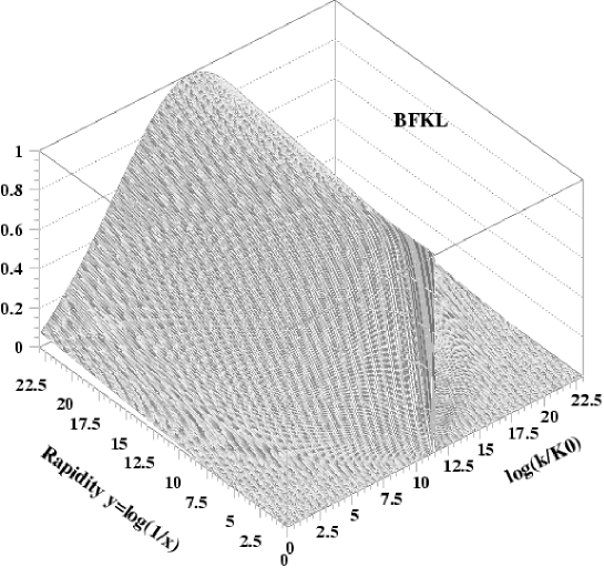
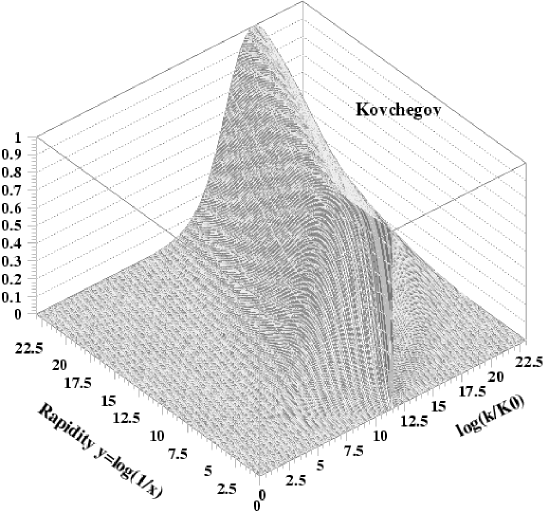
Figure 3: The re-normalized solutions $\Psi(k,Y)$ from the input (11) for the BFKL and the Balitsky-Kovchegov equations as a function of the rapidity $Y$ and $\eta=\ln(k/k_{0})$ with $k_{0}=10^{-10}\;\rm GeV$

The impact of unitarization of the BFKL pomeron on the infra-red behaviour is also illustrated in Fig. 3. These three dimensional plots show the function

$$\Psi(k,Y)\,=\,\frac{k\,\phi(k,Y)}{k_{max}(Y)\,\phi(k_{max}(Y),Y)},$$ (12)

where $k_{max}(Y)$ is the value of the transverse momentum at which $k\,\phi(k,Y)$ has maximum. Thus, $k\,\phi(k,Y)$ is re-normalized to unity at $k=k_{max}$. For the linear BFKL equation, when the asymptotic form sets in, $\Psi(k,Y)$ is given by the second exponent in (10). In this case $k_{max}$ is independent of $Y$ and equal to the scale introduced by the initial condition,

$$k_{max}(Y)\,=\,k_{1}.$$ (13)

For the non-linear case, $\Psi(k,Y)$ moves away of the infra-red region with $k_{max}(Y)$ depending on $Y$. This effect is also shown in Fig. 4 by making projection of constant values of $\Psi(k,Y)$ on the $(\eta,Y)$-plane. Again, for small $Y$, when the non-linearity in the BK equation is negligible, the re-normalized solutions of the BFKL and the BK equations coincide. With increasing Y, when the non-linear effects become important, the difference between them in the region of small $k$ becomes fully visible.

Notice the parallel straight lines of constant values of the non-linear solution in a certain region of the plane in Fig. 4. This means that $\Psi(k,Y)$ in this region is a function of the combination

$$\xi\,=\,\ln(k/k_{0})\,-\,\lambda\,Y\,=\,\ln\left(\frac{k}{k_{0}\exp(\lambda Y)}\right)~{}~{}~{}~{}~{}~{}~{}~{}~{}~{}~{}~{}~{}\lambda>0$$ (14)

(or $e^{\,\xi}$) instead of $k$ and $Y$ separately.

The parameter $\xi$ enumerates different straight lines and it is a matter of convention which line corresponds to $\xi=0$. By a simple rescaling $\xi\rightarrow\xi+\xi_{0}$, (equivalent to the transformation $k_{0}\rightarrow k_{0}e^{-\xi_{0}}$) we can achieve that the straight line part of $k_{max}(Y)$ corresponds to $\xi=0$. In this case the re-normalized solution is a function of only one variable $k/k_{max}(Y)$. The solution of eq. (8) has the same scaling property,

$$\phi(k,Y)=\phi(k/k_{max}(Y))\;,$$ (15)

if and only if

$$\phi(k_{max}(Y),Y)\,=\,\mbox{\rm const}\;,$$ (16)

as a function of $Y$. As shown in Fig. 5, this condition holds true for sufficiently large values of $Y$. In this case the saturation scale can be defined

$$Q_{s}(Y)\equiv k_{max}(Y)\,=\,Q_{0}\exp(\lambda Y)\,,$$ (17)

with the exponential dependence on rapidity governed by the value of the scaling parameter $\lambda$. The pre-factor $Q_{0}$ depends on the initial condition for eq. (8) while the $Y$-dependence is universal. This is illustrated in Fig. 6 where the slope of the straight lines (i.e. the value of $\lambda$) in the scaling region is the same for two different initial distributions, i.e. that given by eq. (11) and the Gaussian distribution

$$k\,\phi(k,Y=0)\,=\,\exp\left[-(\eta-\eta_{1})^{2}/\beta^{2}\right].$$ (18)

We have verified this statement for different values of the parameters $\eta_{1}$ and $\beta$.

It is tempting to claim that for $\xi<0$, i.e. for $k<Q_{s}(Y)$, scaling holds while for $\xi>0$ it is violated. The sharp boundary, however, does not appear in reality and the transition between these two regions is smooth. This is shown in Fig. 7 where the function $k/Q_{s}(Y)\,\phi(k,Y)$ is plotted as a function of the scaling variable $k/Q_{s}(Y)$ for different values of the rapidity $Y$. The scaling behaviour is represented by a common line to the left of the point $k/Q_{s}(Y)=1$. The slow departure from scaling for $k>Q_{s}(Y)$ is clearly visible. In this sense the line $k=Q_{s}(Y)$ is only an approximation characterizing the position of the transition region in the $(k,Y)$-plane. However, the choice based on the position in $k$ of the maximum of $k\phi(k,Y)$ as a function of $Y$ is the most natural one.

Let us finish by recalling that the scaling property of the solution of the BK equation results in the scaling law for the $\gamma^{*}p$ total cross section $\sigma_{\gamma^{*}p}\sim F_{2}/Q^{2}$,

$$\sigma_{\gamma^{*}p}(x,Q^{2})\,=\,\sigma_{\gamma^{*}p}(Q^{2}/Q_{s}^{2}(Y)).$$ (19)

Such scaling law (“geometric scaling”) was found in the small-$x$ DIS data [25].

4 Analytical insight

The emergence of scaling and the saturation scale may also be investigated using the analytic method proposed in [27]. Let us introduce the Mellin transform of the solution $\phi(k,Y)$ of eq. (8):

$$\tilde{\phi}(k,\omega)\,=\,\int dY\,e^{-\omega Y}\phi(k,Y)$$ (20)

where $\omega$ is the Mellin variable conjugated to the rapidity $Y$. We adopt the following ansatz proposed in ref. [27]

$$\tilde{\phi}(k,\omega)\,=\,\tilde{\phi}(\omega)\,e^{(\gamma(\omega)-1)t},$$ (21)

where $\gamma(\omega)$ is anomalous dimension and $t=\ln(k^{2}/k_{0}^{2})$. By taking the Mellin transform of eq. (8), we find

$$\left\{\omega-\bar{\alpha_{s}}\chi(\gamma(\omega))\right\}\,\tilde{\phi}(\omega)\,e^{(\gamma(\omega)-1)t}\,=\,-\overline{\alpha}_{s}\int{d\omega^{\prime}\over 2\pi i}\;\tilde{\phi}(\omega-\omega^{\prime})\,\tilde{\phi}(\omega^{\prime})\,e^{(\gamma(\omega-\omega^{\prime})+\gamma(\omega^{\prime})-2)t}\,,$$ (22)

where $\chi(\gamma)$ is eigenvalue of the leading BFKL kernel

$$\chi(\gamma)\,=\,2\psi(1)\,-\,\psi(\gamma)\,-\,\psi(1-\gamma)\;,$$ (23)

and $\psi$ is the Euler digamma function. The right hand side of eq. (22) can be evaluated in the saddle point approximation [27], which results in

$$\left\{\omega-\bar{\alpha_{s}}\chi(\gamma(\omega))\right\}\,\tilde{\phi}(\omega)\,e^{(\gamma(\omega)-1)t}\,=\,-\overline{\alpha}_{s}\,\tilde{\phi}^{2}(\omega/2)\,e^{(2\gamma(\omega/2)-2)t}\,{1\over\sqrt{4\pi\gamma^{\prime\prime}(\omega/2)t}}\,.$$ (24)

In the region where the non-linear term in (24) can be neglected, the anomalous dimension $\gamma(\omega)$ fulfils the equation

$$\omega-\bar{\alpha_{s}}\chi(\gamma(\omega))\,=\,0\,.$$ (25)

In the double logarithmic approximation, the dominant contribution to $\chi(\gamma)$ comes from the pole $1/\gamma$, and the solution for the anomalous dimension reads

$$\gamma(\omega)\,=\,{\alpha_{s}}/{\omega}\,.$$ (26)

On the other hand, in the saturation region, where the nonlinearity cannot be neglected, the following condition is obtained from eq. (24)

$$\gamma(\omega)\,=\,2\gamma\left({\omega/2}\right)-1\,,$$ (27)

which is satisfied by

$$\gamma(\omega)\,=\,C\,\omega+1\;,$$ (28)

where $C$ is a constant [27].

Using (28) and (21) and performing the inverse Mellin transform in $\omega$, we find the solution to the BK equation in the saturation region

$$\phi(k,Y)\,=\,\int{\frac{d\omega}{2\pi i}}\,e^{\omega Y}\tilde{\phi}(k,\omega)\,\,=\,\int{\frac{d\omega}{2\pi i}}\,\tilde{\phi}(\omega)\,e^{\omega(Ct+Y)}.$$ (29)

We see that the solution $\phi(k,Y)$ depends only on the following combination,

$$C\,t+Y\,=\,2C\,\left[\ln(k/k_{0})+\frac{1}{2C}Y\right],$$ (30)

which is related in a simple way to the previously defined quantity $\xi$, eq. (14), with the scaling parameter $\lambda=-1/(2C)$. In this way the scaling behaviour, seen in the numerical analysis presented in the previous section, is found.

The solutions to eqs. (25) and (27), as well as their derivatives with respect to $\omega$, should match at some $\omega=\omega_{c}$ (see [27] for a full discussion). This allows to fix the value of the unknown parameter $C$ in (30). From (28) one finds

$$\frac{d\gamma(\omega)}{d\omega}\,=\,\frac{\gamma(\omega)-1}{\omega},$$ (31)

and the same relation should be valid for the solution $\gamma(\omega)$ of eq. (25) at $\omega=\omega_{c}$. Thus, by differentiation of eq. (25) with respect to $\omega$, we find

$$\frac{d\chi(\gamma_{c})}{d\gamma}\,=\,-\frac{\chi(\gamma_{c})}{1-\gamma_{c}}\,,~{}~{}~{}~{}~{}~{}~{}~{}~{}~{}~{}~{}~{}~{}~{}~{}~{}~{}~{}~{}~{}~{}\omega_{c}\,=\,\ \overline{\alpha}_{s}\chi(\gamma_{c})\,.$$ (32)

In the DLA, when $\chi(\gamma)=1/\gamma$, one obtains

$$\gamma_{c}={\frac{1}{2}}\,,~{}~{}~{}~{}~{}~{}~{}~{}~{}~{}~{}~{}~{}~{}~{}~{}\omega_{c}=2\,\overline{\alpha}_{s}\,,~{}~{}~{}~{}~{}~{}~{}~{}~{}~{}~{}~{}~{}~{}~{}~{}C={-\frac{1}{4\,\overline{\alpha}_{s}}}\,.$$ (33)

Thus the scaling parameter $\lambda=-1/(2C)=2\,\overline{\alpha}_{s}$. In the case of the BK equation with the full BFKL kernel, we found numerically that the scaling parameter equals

$$\lambda\,=\,2.05\,\overline{\alpha}_{s}\,.$$ (34)

This value is very close to the DLA value and the results quoted in [20] and [23]. We have also checked that (34) still holds in the case of collinear approximation to the BFKL kernel, i.e. keeping only $1/\gamma$ and $1/(1-\gamma)$ poles in eq. (23).

Summarizing, the non-linear BK equation has three regimes depending on the relative importance of the non-linear term: (I) the linear regime (when $k^{2}>Q_{s}^{2}(Y)$) is dominated by the conventional BFKL evolution characterized by the BFKL intercept and diffusion in transverse momenta. In the DLA, the equation is driven by the $1/\gamma$ pole of the kernel eigenvalue (23); (II) in the saturated regime ($k^{2}<Q_{s}^{2}(Y)$), the non-linear effects are strong and the gluon density is saturated. In this case, in the linear part of the BK equation the $1/(1-\gamma)$ pole of $\chi(\gamma)$ is important; (III) the transition between the linear and saturated regimes is defined by the matching (32) which depends on the detailed form of the evolution kernel.

5 The running coupling effects

The inclusion of the running QCD coupling (RC) into the leading order BFKL formalism can be treated as a partial, phenomenological way to account for a part of important non-leading effects. The results of the next-to-leading logarithmic calculations [2] may be invoked to motivate such approach [28, 29, 30]. In the context of the infra-red diffusion, the RC BFKL equation exposes serious problems, in particular, large sensitivity to the treatment of the non-perturbative region. The main result of the forthcoming analysis of the BK equation with the running coupling is that in this case the ambiguities related to the treatment of the infra-red domain are substantially reduced.

The BFKL equation explicitly takes into account the contribution from the momenta down to $k^{2}=0$. Certainly, this is beyond the applicability of the perturbative formalism. Moreover, for the BFKL equation with the running coupling, a purely mathematical difficulty arises due to the Landau pole

$$\alpha_{s}(k^{2})\,=\,{\frac{4\pi}{b_{0}\,\ln{(k^{2}/\Lambda^{2})}}}.$$ (35)

with $b_{0}=11-2n_{f}/3$. Therefore, a cut-off $k_{0}$ for gluon virtualities has to be introduced below which $\alpha_{s}$ is frozen or set to vanish. However, the BFKL amplitude becomes strongly sensitive to the choice of the cut-off. In the case of $\alpha_{s}(k^{2})=0$ for $k^{2}<k_{0}^{2}$, the BFKL kernel with running coupling has a discrete, cut-off dependent spectrum. The largest eigenvalue $\lambda_{max}$, which governs the high energy behaviour of the scattering amplitude, is bounded by [31]:

$$\frac{3.6}{\pi}\alpha_{s}(k_{0}^{2})\,\leq\,\lambda_{max}\,\leq\,{\frac{12\ln{2}}{\pi}}\alpha_{s}(k_{0}^{2}).$$ (36)

From this, one concludes that the equation is unstable, i.e. the pomeron intercept may reach an arbitrarily large value depending on the infra-red cut-off. Besides, it was found that the solution $\phi(k,Y)$ of the BFKL equation with the running coupling no longer exhibits the diffusion pattern typical for the fixed coupling case. Namely, it takes the following factorized form for sufficiently large $Y$ and $k^{2}>k_{0}^{2}$ [32]:

$$k\phi(k,Y)\,\sim\,\exp\{\lambda Y\}\,{\frac{1}{k}}\,[\ln\left({k^{2}}/{k_{0}^{2}}\right)]^{\nu},$$ (37)

with $\lambda=\lambda_{max}$ and $\nu=12/(11\lambda)-1$, so that $\nu$ is positive for moderate $\lambda$ and becomes negative for $\lambda>12/11$. Thus, diffusion into infra-red is strongly enhanced in the running coupling case, keeping the gluon chains in the region of small virtualities. As a result, the high energy behaviour is governed by the non-perturbative part of the gluon configurations. However, it is still possible to perform collinear factorization in which the genuine non-perturbative contribution may be absorbed into the input for the evolution in $Q^{2}$ [33].

The BK equation is also of perturbative origin so its validity at low $k^{2}$ may be questioned. However, the equation is strongly constrained by unitarity requirements. In particular, the demand for the dipole scattering amplitude to saturate to unity for large dipoles (the scattering matrix in the forward direction $S=0$ for large dipoles) results in a universal form of $\phi(k,Y)\sim\ln k$ for small $k$ and fixed $Y$. The statement about the large $r$ behaviour of the dipoles is quite general. Interestingly, the Balitsky-Kovchegov equation, which is rooted in perturbative QCD, ensures such behaviour of the solutions at large $r$.

This conclusion remains unaltered also in the scenario with the running coupling. The unitarity effects are strongest in the region of small values of the gluon momenta. This is due to the fact that the solution to the linear part of eq. (8) is proportional to $k^{-1}$ in the fixed coupling case, (eq. 10), and it rises faster towards low $k$ making the non-linear rescattering term largest for small $k$. This effect tames the rapid rise of the amplitude governed by the running coupling taken at the cut-off scale $k_{0}^{2}$. The evolution for low $k$ is essentially frozen to the known form and it is the perturbative region of $k$ which drives the evolution. This was noticed in [18] as a supersaturation phenomenon.

In Fig. 8 a,b we show the results of the numerical investigation of the BK equation (8) with the running coupling. We considered two scenarios: the cut-off regularization of the running coupling,

$$\alpha_{s}(k^{2})=0~{}~{}~{}~{}~{}~{}~{}~{}~{}~{}\mbox{\rm for}~{}~{}~{}~{}~{}~{}~{}~{}~{}~{}k^{2}<k_{0}^{2}\,,$$ (38)

and freezing of the running coupling at low scales

$$\alpha_{s}\,(k^{2})\,\,\,\rightarrow\,\,\,\alpha_{s}(k^{2}+k_{0}^{2})\,.$$ (39)

The latter option is supported by some solid theoretical arguments [34] and the QCD lattice data, see e.g. ref. [35]. The argument $k^{2}$ is given by the virtuality of the outgoing exchanged gluon, see Fig. 1, and the same $\alpha_{s}(k^{2})$ is assumed in the linear and non-linear terms. A different choice of the scale would correspond to a modification of the BFKL kernel in the NLL approximation [2, 28] which does not influence significantly the properties of the solution. In order to investigate the sensitivity to infra-red details, two values of the cut-off were used: $k_{0}^{2}=0.1~{}\mbox{\rm GeV}^{2}$ (a) and $k_{0}^{2}=1~{}\mbox{\rm GeV}^{2}$ (b). Both scenarios for the running coupling lead to similar results. The contours of constant values of the function $\Psi(k,Y)$, eq. (12), in the scenario (38) are plotted in the $(\eta,Y)$-plane. The input is given by the Gaussian (18) centered at $k_{1}=10^{2}$ GeV.

We see in Figs. 8 that the solution to the BFKL equation passes through a rapid “tunnelling” transition (the detailed discussion of this phenomenon is presented in [30]), collapsing from the region of $k\simeq k_{1}$(input scale) to $k\simeq k_{0}$ (cut-off scale) at certain rapidity. As expected, for larger $Y$ the shape in $k$ factors out from the $Y$-dependence for the solution of the BFKL equation $\phi(k,Y)$. In the re-normalized solution $\Psi(k,Y)$, eq. (12), the $Y$-dependence drops out and the lines of constant values become parallel to the $Y$-axis, as seen in Fig. 8.

The behaviour of the solution of the non-linear BK equation is different. Now, we distinguish three regimes for $\Psi(k,Y)$:

• For small Y, the linear BFKL regime occurs with diffusion weighted towards low $k$.

• When $Y$ increases, the distributions broadens and the tunnelling transition occurs. However, this effects is different from the collapse observed in the linear BFKL case since the saturation scale is generated which suppresses $\Psi(k,Y)$ for small $k$.

• For high $Y$, geometric scaling (15) appears. The saturation scale increases with $Y$ and the dynamics of evolution is governed by perturbative values of $k$.

The dependence on the cut-off $k_{0}$ is marginal for large $Y$ in both the saturated and the non-saturated range of $k$. The statement about the independence from the infra-red parameter $k_{0}$ also holds for the effective intercept which governs the increase of the gluon density with $Y$ for the scales much larger than the saturation scale $Q_{s}(Y)$.

It is interesting to estimate how the running coupling affects the $Y$ dependence of the saturation scale $Q_{s}(Y)$. We adopt a natural approximation that the local exponent $\lambda(Y)=d\ln(Q_{s}(Y)/\Lambda)\;/dY$ takes the form $\lambda(Y)=2\bar{\alpha}_{s}(Q^{2}_{s}(Y))$ where $\Lambda=\Lambda_{QCD}$. The above form is motivated by the leading logarithmic result with the fixed coupling (33) and its numerical verification (34). Thus, we have

$${d\ln(Q_{s}(Y)/\Lambda)\over dY}={12\over b_{0}\ln(Q_{s}(Y)/\Lambda)}\,,$$ (40)

with the initial condition $Q_{s}(Y_{0})=Q_{0}$ and $Y_{0}$ chosen in the region where scaling sets in. The solution takes the form

$$Q_{s}(Y)=\Lambda\;\exp\left(\sqrt{{24\over b_{0}}\,(Y-Y_{0})+L_{0}^{2}}\right)\,,\qquad Y>Y_{0}\,,$$ (41)

where $L_{0}=\ln(Q_{0}/\Lambda)$. It follows that the local exponent $\lambda(Y)$ decreases with increasing rapidity, and $\lambda(Y)\sim 1/\sqrt{Y}$ for very large $Y$. Such dependence is indeed seen in the numerical analysis.

In Fig. 9 we illustrate scaling in the running coupling case by showing the function $(k/Q_{s}(Y))\,\phi(k,Y)$ plotted versus $k/Q_{s}(Y)$ for different values of rapidity. $Q_{s}(Y)$ is given by formula (41) with the initial condition $Q_{s}(Y=0)=2~{}\mbox{\rm GeV}$. The overlapping curves at low values of the scaling variable clearly indicate that for $k<Q_{s}(Y)$ scaling is satisfied to a very good accuracy, thus justifying our ansatz (41) for the saturation scale.

Summarizing, the Balitsky-Kovchegov equation avoids the self-consistency problems of the BFKL equation when the running coupling is included. The sensitivity to the treatment of the infra-red region is much smaller than in the linear case due to the appearance of the saturation scale. In contrast to the BFKL equation with the running coupling, the large $Y$ asymptotics of the dipole scattering amplitude arising from the BK equation is governed by gluon virtualities in the perturbative domain.

6 The kinematic constraint effects

The BK equation (4) has been derived in the leading logarithmic approximation. It has been argued that the NLL corrections should be smaller that the saturation effects embodied in this equation. Since the corrections from the NLL BFKL kernel become important at rapidities $Y_{NLL}\sim 1/\alpha_{s}^{5/3}$, they should be parametrically smaller than the unitarity corrections which enter at rapidities of the order $Y_{U}\sim 1/\alpha_{s}\ln(1/\alpha_{s})$. However, it is well known that the next-to-leading corrections [2] to the BFKL kernel are numerically important and even make the high energy expansion unstable. Namely, the pomeron intercept in the NLL order,

$$\omega_{NLL}\;\simeq\;4\ln 2\;\overline{\alpha}_{s}\,(1-6.47\,\overline{\alpha}_{s})\,,$$ (42)

becomes negative already for small value of $\overline{\alpha}_{s}\simeq 0.16$ [2]. These problems have been solved in [28] where a method which stabilizes the high energy expansion by a proper resummation of collinear and energy-scale-dependent terms to all orders has been proposed. As a result, one obtains a renormalization and resummation scheme independent equation. Similar approaches have also been developed in [36, 37]. In the previous section we have studied the NLL corrections due to the running of the coupling $\alpha_{s}$. Here, we study different subleading effects, namely those coming from the change of the energy scale.

In order to verify the importance of the NLL terms we shall modify the BK equation in momentum space (8) by imposing so called kinematic constraint [38, 39] (see fig. 1),

$$k^{\prime 2}\,<\,k^{2}/z$$ (43)

on the real emission term in the linear part of the BK equation. The origin of this constraint lies in the fact that in the multi-Regge kinematics the exchanged gluon virtuality is dominated by its transverse momentum, $|k^{\prime 2}|\simeq|k_{T}^{2}|$. After imposing the kinematical constraint one arrives at the following modified BK equation

$$\phi(k,Y)=\phi_{0}(k) + \overline{\alpha}_{s}\int_{0}^{Y}dy\left[\int_{0}^{\infty}\frac{dk^{\prime 2}}{k^{\prime 2}}\,\right.\left\{\frac{k^{\prime 2}\phi(k^{\prime},y)\,\Theta(Y-y-\ln(k^{\prime 2}/k^{2}))\,-\,k^{2}\phi(k,y)}{|k^{2}\,-\,k^{\prime 2}|}\right.$$ (44)

$$+ \left.\left.\frac{k^{2}\,\phi(k,y)}{\sqrt{4k^{\prime 4}\,+\,k^{4}}}\right\}\,-\,\phi^{2}(k,y)\right]\,,$$

where $y=\ln(z/x)$ and $Y-y=\ln(1/z)$, see Fig. 1. The function $\phi_{0}(k)$ is an initial condition at $Y=0$. Notice that we no longer deal with a differential equation in rapidity, compare eq. (8).

Condition (43) leads to the following modification of the leading eigenvalue (23) of the BFKL kernel

$$\chi(\gamma,\omega)\;=\;2\psi(1)-\psi(\gamma)-\psi(1-\gamma+\omega)\,,$$ (45)

where $\gamma$ and $\omega$ are the Mellin variables conjugated to $\ln k^{2}/\Lambda^{2}$ and $Y$, respectively. The indicated shift in the second $\psi$ function accounts for the resummation to all orders of subleading terms resulting from the changes of the energy scale. The obtained $\omega$-dependent kernel ensures that the collinear limits are always correctly reproduced [28, 40]. The new Pomeron intercept $\omega_{NLL}$ stays always positive and is significantly reduced as compared to the leading logarithmic value $\omega_{LL}=4\ln 2\,\overline{\alpha}_{s}$ [28, 39]. It also depends non-linearly on $\bar{\alpha}_{s}$ which is a consequence of the $\omega$ dependence of the eigenvalue (45).

The solution of the BK equation with the kinematic constraint also exhibits the previously discussed scaling property. Repeating the analysis of Section 4 with the BFKL kernel eigenvalue $(\ref{eq:chiom})$ instead of $(\ref{eq:eigenvalue})$, we arrived at the scaling condition in the saturation region with the variable (30). Now, the value of the scaling parameter $\lambda$ is different. The matching condition (32) is replaced by

$$\frac{\partial\chi}{\partial\gamma_{c}}\,=\,-\frac{\chi}{1-\gamma_{c}}\,\left(1-\overline{\alpha}_{s}\,\frac{\partial\chi}{\partial\omega_{c}}\right)\,,~{}~{}~{}~{}~{}~{}~{}~{}~{}~{}~{}~{}~{}~{}~{}\omega_{c}\,=\,\ \overline{\alpha}_{s}\chi(\gamma_{c},\omega_{c})\,.$$ (46)

Let us consider the DL approximation in which the eigenvalue (45) is expanded in $\gamma$ and then in $\omega$ around $\gamma=\omega=0$

$$\chi(\gamma,\omega)\simeq{1\over\gamma}-{\pi^{2}\over 6}\omega\,.$$ (47)

Using this form of the BFKL eigenvalue in the matching conditions (46), we find

$$\gamma_{c}={\frac{1}{2}}\,,~{}~{}~{}~{}~{}~{}~{}~{}~{}~{}~{}~{}~{}~{}~{}~{}\omega_{c}={2\,\overline{\alpha}_{s}\over 1+\pi^{2}\bar{\alpha}_{s}/6}\,,~{}~{}~{}~{}~{}~{}~{}~{}~{}~{}~{}~{}~{}~{}~{}~{}C=-{1+\pi^{2}\overline{\alpha}_{s}/6\over 4\,\overline{\alpha}_{s}}\,,$$ (48)

which should be compared to the result (33) for the BK equation with the linear kernel without the kinematic constraint. Now, the scaling parameter $\lambda=-1/(2C)$ reads

$$\lambda={2\,\overline{\alpha}_{s}\over 1+\pi^{2}\overline{\alpha}_{s}/6}.$$ (49)

This approximate result suggests that the scaling parameter is reduced in comparison with the standard BK equation, see eq. (34). Moreover, the dependence of $\lambda$ on $\bar{\alpha}_{s}$ is non-linear.

We have solved numerically the BK equation (8) with the kinematic constraint in the BFKL kernel and found that indeed the scaling property approximately holds. The scaling parameter $\lambda$ is found to be reduced with respect to the value (34) for the BK equation without the kinematic constraint. The non-linear dependence on $\bar{\alpha}_{s}$ of the form (49) is confirmed by the numerical considerations within some $15\%$ relative deviation, towards smaller values of $\lambda$.

In Fig. 9 we show the solution $\phi(k,Y)$ of the BK equation with and without the kinematic constraint as a function of $k$ for different values of $Y$. In both cases the same Gaussian input (18) concentrated at $k_{1}=1\,{\rm GeV}$ is used. The overall pattern is similar in both cases, with power-like fall for the large values of $k$ and the $\ln(k/k_{0})$ behaviour for small values of $k$. However, the transition between the two regimes at the same values of rapidity occurs for smaller values of $k$ in the case of solution with the kinematic constraint. This means that the saturation scale generated by the BK equation is smaller when the kinematic constraint is present. This is a phenomenon analogous to the well known reduction of the leading order BFKL pomeron intercept by including the next-to-leading corrections.

From Fig. 9 it is seen that the kinematic constraint is potentially very important for the phenomenological studies based on the BK equation. Its effect manifests for instance in a slower increase of the saturation scale than in the standard case. The impact of the kinematic constraint is even more important in the linear regime, where the solution $\phi(k,Y)$ drops by two orders of magnitude at $Y=20$ (for $\alpha_{s}=0.2$) when the constraint is included. However, the general picture of the saturation process remains unaltered. So, future reliable phenomenological applications of the BK equation to should involve the kinematic constraint or another representation of resummed non-leading corrections to the BFKL part of the evolution kernel. It might also be valuable to combine the kinematic constraint and the running coupling effects in the BK equation.

7 Summary

We presented detailed numerical analysis of the non-linear Balitsky-Kovchegov (BK) equation. We showed how diffusion into the infra-red domain for the linear BFKL equation is suppressed for the BK equation due to the emergence of the saturation scale $Q_{s}(Y)$, which depends on the rapidity $Y$. The saturation scale divides the $(k,Y)$-plane into a region governed by the linear BFKL evolution when $k>Q_{s}(Y)$, and the region in which gluon saturation occurs when $k<Q_{s}(Y)$. In the latter region, the solution is a function of only one variable $k/Q_{s}(Y)$, instead of $k$ and $Y$ separately (scaling behaviour). Our results are fully compatible with the previous analyses performed at the leading order. The scaling parameter $\lambda\approx 2\bar{\alpha_{s}}$ which governs the $Y$ dependence of the saturation scale, $Q_{s}\sim\exp{(\lambda Y)}$, is universal and does not depend on the form of the initial conditions for the evolution.

We also investigated the influence of the NLL corrections to the BFKL kernel such as the running coupling and kinematic constraint. Similarly to the fixed coupling case, when $\alpha_{s}$ runs, the diffusion of gluon virtualities into the infra-red domain is avoided by generation of the saturation scale $Q_{s}$. We found, however, a different dependence of $Q_{s}$ on the rapidity, see eq. (41). Thus, the non-linear evolution at high rapidity is driven by gluon momenta in the perturbative range independently of the initial condition for the evolution. The details of the BK solutions in the running coupling case are quite insensitive to the regularization of $\alpha_{s}$ at small scales.

We also studied the impact of the kinematic constraint onto the non-linear BK equation and found that an approximate scaling property still holds. However, the kinematic constraint slows down the rise of the gluon density with increasing rapidity (energy). Thus, the saturation scale increases slower with rapidity than in the unconstrained case, see eq. (49).

We derived and tested numerically the analytic formulae describing the dependence of the saturation scale on rapidity when either the kinematic constraint or the running QCD coupling are included in the BK equation. This is the first systematic study of impact of those subleading corrections on the gluon density saturation in the Balitsky-Kovchegov framework. These results suggest that the subleading effects are very important for the construction of a reliable phenomenology.

Figure 2: The functions $k\phi(k,Y)$ constructed from solutions to the BFKL and the Balitsky-Kovchegov equations with the input (11) for different values of the evolution parameter $Y=\ln(1/x)$ ranging from $1$ to $10$. The coupling constant $\alpha_{s}=0.2$.

Figure 4: The lines of constant values of the BFKL and the BK re-normalized solutions $\Psi(k,Y)$ ($Y=\ln(1/x)$) in the $(\log_{10}(k),\log_{10}(1/x))$-plane.

Figure 5: Scaling condition (16) as a function of $Y$.

Figure 6: The lines of constant values of the Balitsky-Kovchegov re-normalized solutions $\Psi(k,Y)$ in the $(\log_{10}(k),\log_{10}(1/x))$-plane for the delta-like input (11) and the Gaussian input (18).

Figure 7: The function $(k/Q_{s}(Y))\,\phi(k,Y)$ plotted versus $k/Q_{s}(Y)$ for different values of rapidity $Y$ ranging from $10$ to $23$. The saturation scale $Q_{s}(Y)$ corresponds to the position of the maximum of the function $k\,\phi(k,Y)$.

Figure 8: The re-normalized solutions $\Psi(k,Y)$ from the input (11) for the Balitsky-Kovchegov equation with the running coupling constant and the infra-red cut-off $k_{0}^{2}=0.1\,\mbox{\rm GeV}^{2}$ (a) and $k_{0}^{2}=1\,\mbox{\rm GeV}^{2}$ (b) as functions of $\log_{10}(1/x)$ and $\log_{10}(k/1\,\mbox{\rm GeV})$.

Figure 9: The function $(k/Q_{s}(Y))\,\phi(k,Y)$ in the running coupling case, plotted versus $k/Q_{s}(Y)$ for different values of rapidity $Y$ ranging from $15$ to $32$. The saturation scale $Q_{s}(Y)$ is taken from equation (41) with the initial condition $Q_{s}(Y=0)=2.0\;GeV$.

Figure 10: Comparison of solutions of the Balitsky-Kovchegov equation with and without the kinematic constraint, plotted versus $k$ for different values of rapidity $Y_{i}=20+i*2$, where $i$ goes from $0$ to $10$. The dotted line – the input distribution at $Y=0$; the solid line – the result of the calculation with the kinematic constraint, the dashed line – the result of the calculation without the kinematic constraint. The coupling constant $\alpha_{s}=0.2$ is fixed.

References

-
[1]
L. N. Lipatov, Sov. J. Nucl. Phys.
23 (1976) 338;
E. A. Kuraev, L. N. Lipatov and V. S. Fadin, Sov. Phys. JETP 45 (1977) 199;
I. I. Balitsky and L. N. Lipatov, Sov. J. Nucl. Phys. 28 (1978) 338. -
[2]
V. S. Fadin, M. I. Kotsky and R. Fiore,
Phys. Lett. B 359, 181 (1995);
V. S. Fadin, M. I. Kotsky and L. N. Lipatov, BUDKERINP-96-92, hep-ph/9704267; V. S. Fadin, R. Fiore, A. Flachi and M. I. Kotsky, Phys. Lett. B 422, 287 (1998);
V. S. Fadin and L. N. Lipatov, Phys. Lett. B 429, 127 (1998);
G. Camici and M. Ciafaloni, Phys. Lett. B 386, 341 (1996); Phys. Lett. B 412, 396 (1997) [Erratum-ibid. B 417, 390 (1997)]; Phys. Lett. B 430, 349 (1998). - [3] L. V. Gribov, E. M. Levin and M. G. Ryskin, Phys. Rep. 100 (1983) 1.
- [4] A. H. Mueller and J. W. Qiu, Nucl. Phys. B268 (1986) 427.
-
[5]
L. McLerran and R. Venugopalan,
Phys. Rev. D49 (1994) 2233;
Phys. Rev. D49 (1994) 3352;
Phys. Rev. D50 (1994) 2225;
R. Venugopalan, Acta Phys. Polon. B30 (199) 3731;
E. Iancu, A. Leonidov and L. McLerran, Nucl.Phys. A692 (2001) 583;
E. Ferreiro, E. Iancu, A. Leonidov and L. McLerran, hep-ph/0109115. - [6] J. Jalilian-Marian, A. Kovner, A. Leonidov and H. Weigert, Nucl. Phys. B504 (1997) 415; Phys. Rev. D59 (1999) 014014; Phys. Rev. D59 (1999) 034007.
- [7] I. I. Balitsky, Nucl. Phys. B463 (1996) 99;
- [8] I. Balitsky, Phys. Rev. Lett. 81 (1998) 2024; Phys. Rev. D60 (1999) 014020; hep-ph/0101042.
- [9] I. I. Balitsky, Phys. Lett. B518 (2001) 235.
- [10] H. Weigert, preprint NORDITA-2000-34-HE, hep-ph/0004044.
- [11] E. Iancu and L. McLerran, Phys. Lett. B510 (2001) 133.
- [12] A.H. Mueller, CU-TP-1031, hep-ph/0110169.
- [13] Yu. V. Kovchegov, Phys. Rev. D60 (1999) 034008.
-
[14]
A. H. Mueller, Nucl. Phys. B415 (1994) 373;
A. H. Mueller and B. Patel, Nucl. Phys. B425 (1994) 471;
N. N. Nikolaev and B. G. Zakharov, Phys. Lett. B332 (1994) 184; Z. Phys. C64 (1994) 631. - [15] J. Bartels and M. Wüsthoff, Z. Phys. C66 (1995) 157.
- [16] Yu. V. Kovchegov, Phys. Rev. D61 (2000) 074018.
- [17] M. A. Braun, Eur. Phys. J. C16 (2000) 337.
- [18] M. A. Braun, hep-ph/0010041.
- [19] E. M. Levin and K. Tuchin, Nucl. Phys. B573 (2000) 833;
- [20] E. M. Levin and K. Tuchin, Nucl.Phys. A691 (2001) 779; Nucl. Phys. A693 (2001) 787.
- [21] E. M. Levin and M. Lublinsky, TAUP-2670-2001 hep-ph/0104108.
- [22] M. Lublinsky, Eur. Phys. J. C21 (2001) 513, hep-ph/0108239.
- [23] N. Armesto and M. A. Braun, Eur. Phys. J. C20 (2001) 517; UCOFIS-4-01, US-FT-10-01, hep-ph/0107114.
- [24] I.I. Balitsky and A.V. Belitsky, hep-ph/0110158.
- [25] A. M. Staśto, K. Golec-Biernat and J. Kwieciński, Phys. Rev. Lett. 86 (2001) 596.
- [26] K. Golec–Biernat and M. Wüsthoff, Phys. Rev. D59 (1999) 014017; Phys. Rev. D60 (1999) 114023; Eur. Phys. J. C20 (2001) 313.
- [27] J. Bartels and E. Levin, Nucl.Phys. B387 (1992) 617.
- [28] M. Ciafaloni, D. Colferai and G. P. Salam, Phys. Rev. D 60 (1999) 114036.
- [29] G. P. Salam, Acta Phys. Polon. B 30 (1999) 3679.
- [30] M. Ciafaloni, D. Colferai and G. P. Salam, JHEP 9910 (1999) 017.
- [31] J. C. Collins and J. Kwieciński, Nucl. Phys. B 316 (1989) 307.
- [32] B. Andersson, G. Gustafson and H. Kharraziha, Phys. Rev. D 57 (1998) 5543.
- [33] J. Kwieciński and A. D. Martin, Phys. Lett. B 353 (1995) 123.
- [34] Yu. A. Simonov, hep-ph/0109081; hep-ph/0109159.
- [35] A. M. Badalian and D. S. Kuzmenko, hep-ph/0104097.
- [36] R.S. Thorne Phys. Rev. D64 (2001) 074005.
- [37] G. Altarelli, R.D. Ball and S. Forte Nucl. Phys. B575 (2000) 313; Nucl. Phys. B599 (2001) 383.
- [38] B. Andersson, G. Gustafson, H. Kharraziha and J. Samuelsson, Z. Phys. C 71 (1996) 613.
- [39] J. Kwieciński, A. D. Martin and P. J. Sutton, Z. Phys. C 71 (1996) 585.
- [40] G. P. Salam, JHEP 9807 (1998) 019.