Abstract

We examine the potential for detecting and studying Higgs bosons at a photon-photon collider facility associated with a future linear collider. Our study incorporates realistic $\gamma\gamma$ luminosity spectra based on the most probable available laser technology. Results include detector simulations. We study the cases of: a) a SM-like Higgs boson; b) the heavy MSSM Higgs bosons; c) a Higgs boson with no $WW/ZZ$ couplings from a general two Higgs doublet model.

1 Introduction

Higgs production in $\gamma\gamma$ collisions, first studied in [1, 2], offers a unique capability to measure the two-photon width of the Higgs and to determine its charge conjugation and parity (CP) composition through control of the photon polarization. Both measurements have unique value in understanding the nature of a Higgs boson eigenstate. Photon-photon collisions also offer one of the best means for producing a heavy Higgs boson singly, implying significantly greater mass reach than $e^{+}e^{-}$ production of a pair of Higgs bosons. In this paper, we present a realistic assessment of the prospects for these studies based on the current Next Linear Collider (NLC) machine and detector designs [3, 4, 5], but we will also comment on changes in our results based on the TeV-Energy Superconducting Linear Accelerator (TESLA) design [6]. When referring to either of these machines in a generic context, we will use the phrase “Linear Collider” (LC). Summaries of and references to other recent work on $\gamma\gamma$ Higgs production at the LC appear in [3, 4, 5, 6]. In our work, we attempt to assess the potential of $\gamma\gamma$ Higgs production using a realistic computation of the luminosity and polarizations of the colliding back-scattered photons and of the resulting backgrounds, including detector simulation and appropriate cuts. We will particularly focus on: a) studying a light Standard-Model-like Higgs boson, including a determination of its CP; and b) determining the best strategy for detecting the heavy Higgs bosons of the MSSM for model parameter choices such that they will not be seen either at the LHC or in $e^{+}e^{-}$ collision operation of the LC.

There are many important reasons for measuring the $\gamma\gamma$ coupling of a Higgs boson, generically denoted $h$. In the Standard Model (SM), the coupling of the Higgs boson, $h_{SM}$, to two photons receives contributions from loops containing any charged particle whose mass arises in whole or part from the vacuum expectation value (vev) of the neutral Higgs field. In the limit of infinite mass for the charged particle in the loop, the contribution asymptotes to a value that depends on the particle’s spin (i.e. the contribution does not decouple). Thus, a measurement of $\Gamma(h_{SM}\to\gamma\gamma)$ provides the possibility of revealing the presence of arbitrarily heavy charged particles, since in the SM context all particles acquire mass via the Higgs mechanism. Of course, since such masses are basically proportional to some coupling times $v=174~{}{\rm GeV}$ (the Higgs field vacuum expectation value), if the coupling is perturbative the masses of these heavy particles are unlikely to be much larger than $0.5-1~{}{\rm TeV}$. Since $BR(h_{SM}\to X)$ is entirely determined by the spectrum of light particles, and is thus not affected by heavy states, $N(\gamma\gamma\to h_{SM}\to X)\propto\Gamma(h_{SM}\to\gamma\gamma)BR(h_{SM}\to X)$ will then provide an extraordinary probe for such heavy states.

Even if there are no new particles that acquire mass via the Higgs mechanism, a precision measurement of $N(\gamma\gamma\to h\to X)$ for specific final states $X$ ($X=b\overline{b},WW^{*},\ldots$) can allow one to distinguish between a $h$ that is part of a larger Higgs sector and the SM $h_{SM}$. The ability to detect deviations from SM expectations will be enhanced by combining this with other types of precision measurements for the SM-like Higgs boson. Observation of small deviations would be typical for an extended Higgs sector as one approaches the decoupling limit in which all other Higgs bosons are fairly heavy, leaving behind one SM-like light Higgs boson. In such models, the observed small deviations could then be interpreted as implying the presence of heavier Higgs bosons. Typically, deviations exceed 5% if the other heavier Higgs bosons have masses below about 400 to 500 GeV. A precise measurement of the deviations, coupled with enough other information about the model, might then allow one to constrain the masses of the heavier Higgs bosons, thereby allowing one to understand how to go about detecting them directly. For example, in the case of the two-doublet minimal supersymmetric Standard Model (MSSM) Higgs sector there are five physical Higgs bosons (two CP-even, $h^{0}$ and $m_{H^{0}}$ with $m_{h^{0}}<m_{H^{0}}$; one CP-odd, $A^{0}$; and a charged Higgs pair, $H^{\pm}$). In this model, significant deviations of the $h^{0}$ properties from those of the $h_{SM}$ would indicate that $m_{A^{0}}$ might well be sufficiently small that the approximately degenerate $H^{0}$ and $A^{0}$ could be discovered in $\gamma\gamma\to H^{0},A^{0}$ production at a LC collider with energy of order $\sqrt{s}=500-600~{}{\rm GeV}$.

Of course, the ability to detect $\gamma\gamma\to H^{0},A^{0}$ will be of greatest importance if the $H^{0}$ and $A^{0}$ cannot be detected either at the Large Hadron Collider (LHC) or in $e^{+}e^{-}$ collisions at the LC. In fact, there is a very significant section of parameter space in the MSSM for which this is the case, often referred to as the ‘wedge’ region. The wedge basically occupies the following region of $m_{A^{0}}$–$\tan\beta$ parameter space.

• $m_{A^{0}}\sim m_{H^{0}}\mathrel{\raise 1.29167pt\hbox{$>$\kern-7.5pt\lower 4.30554pt\hbox{$\sim$}}}\sqrt{s}/2$, for which $e^{+}e^{-}\to H^{0}A^{0}$ pair production is impossible — we will be focusing on an LC with $\sqrt{s}=630~{}{\rm GeV}$, implying that the wedge begins at $m_{A^{0}}<315~{}{\rm GeV}$.

• $\tan\beta>3$ — below this, the LHC will be able to detect the $H^{0},A^{0}$ in a variety of modes such as $H^{0}\to h^{0}h^{0}$ and $A^{0}\to Zh^{0}$ for $m_{A^{0}}\mathrel{\raise 1.29167pt\hbox{$<$\kern-7.5pt\lower 4.30554pt\hbox{$\sim$}}}2m_{t}$ and $H^{0},A^{0}\to t\overline{t}$ for $m_{A^{0}}\mathrel{\raise 1.29167pt\hbox{$>$\kern-7.5pt\lower 4.30554pt\hbox{$\sim$}}}2m_{t}$. In some versions of the MSSM (e.g. the maximal mixing scenario), most of this region is already eliminated by constraints from the Large Electron Positron Collider (LEP) data.

• $\tan\beta<\tan\beta^{\rm min}(m_{A^{0}})$, where $\tan\beta^{\rm min}(m_{A^{0}})$ is the minimum value of $\tan\beta$ for which the LHC can detect $b\overline{b}H^{0}+b\overline{b}A^{0}$ production in the $A^{0},H^{0}\to\tau^{+}\tau^{-}$ decay modes (currently deemed the most accessible) — $\tan\beta^{\rm min}(m_{A^{0}})$ rises from $\sim 12$ at $m_{A^{0}}=315~{}{\rm GeV}$ to $\sim 18$ at $m_{A^{0}}=500~{}{\rm GeV}$.

• In this wedge, the LC alternatives of $e^{+}e^{-}\to b\overline{b}H^{0}$ and $e^{+}e^{-}\to b\overline{b}A^{0}$ production also have such extremely small rates as to be undetectable — see, e.g. [8].

This wedge will be discussed in greater detail later in the paper. A LC for which the maximum $e^{+}e^{-}$ center of mass energy is $\sqrt{s}=630~{}{\rm GeV}$ can potentially probe Higgs masses in $\gamma\gamma$ collisions as high as $\sim 500~{}{\rm GeV}$, the point at which the $\gamma\gamma$ luminosity spectrum runs out. An important goal of this paper is to determine the portion of the ‘wedge’ $[m_{A^{0}},\tan\beta]$ parameter region for which $H^{0},A^{0}$ will be detectable via $\gamma\gamma$ collisions. We find the following.

• If $m_{H^{0}}$ and $m_{A^{0}}$ are known to within roughly $50~{}{\rm GeV}$ on the basis of precision $h^{0}$ data (and there is sufficient knowledge of other MSSM parameters from the LHC to know how to interpret these data), then we find that it is almost certain that we can detect the $H^{0}$ and $A^{0}$ by employing just one or two $\sqrt{s}$ settings and electron-laser-photon polarizations such as to produce a $\gamma\gamma$ spectrum peaked in the region of interest.

• However, it is very possible that there will be no fully reliable constraints on the $H^{0},A^{0}$ masses (other than $m_{A^{0}}\sim m_{H^{0}}>\sqrt{s}/2$ from LC running in the $e^{+}e^{-}$ collision mode). In this case, for expected luminosities, the simplest, and probably also the most efficient, procedure will be to simply operate the machine at a single (high) energy, roughly 2/3 to 3/4 of the time using electron-laser-photon polarization configurations that produce a broad spectrum $E_{\gamma\gamma}$ spectrum and 1/3 to 1/4 of the time using configurations that yield a spectrum peaked at high $E_{\gamma\gamma}$. We will find that after three to four years of operation this procedure will yield a visible signal for $H^{0},A^{0}$ production for most of the wedge parameter space, and, more generally, for many $[m_{A^{0}},\tan\beta]$ parameter choices.

Earlier work on detecting the heavy MSSM Higgs bosons in $\gamma\gamma$ collisions appears in ([9, 10]. Our study employs the best available predictions for the $\gamma\gamma$ luminosity spectrum and polarizations using the realistic assumption of 80% polarization for the colliding electron beams.

The $\gamma\gamma$ collider would also play a very important role in exploring a non-supersymmetric general two-Higgs-doublet model (2HDM). In this paper, we will explore the role of a $\gamma\gamma$ collider in the context of a CP-conserving (CPC) type-II  2HDM (of which the MSSM Higgs sector is a special case). In particular, there are CPC type-II 2HDM’s with Higgs sector potentials for which the lightest Higgs boson is not at all SM-like, despite the fact that the other Higgs bosons are fairly heavy. Several such models were considered in Ref. [11]. In the models considered, there is a light Higgs boson with no $WW,ZZ$ coupling, generically denoted $\widehat{h}$, while all other Higgs bosons (including a heavy neutral Higgs boson with SM-like couplings) are heavier than $\sqrt{s}$. Further, there is a wedge (somewhat analogous to, but larger than, that of the MSSM) of moderate $\tan\beta$ values in which the $e^{+}e^{-}\to b\overline{b}\widehat{h}$ and $e^{+}e^{-}\to t\overline{t}\widehat{h}$ production processes both yield fewer than 20 events for $L=1~{}{\rm ab}^{-1}$ and in which LHC detection will also be impossible. If $m_{\widehat{h}}$ is also so heavy ($m_{\widehat{h}}>150~{}{\rm GeV},250~{}{\rm GeV}$ for $\sqrt{s}=500~{}{\rm GeV},800~{}{\rm GeV}$, respectively) as to yield few or no events in $e^{+}e^{-}\to Z\widehat{h}\widehat{h}$ or $e^{+}e^{-}\to\nu\overline{\nu}\widehat{h}\widehat{h}$ production, then only $\gamma\gamma\to\widehat{h}\to b\overline{b}$ might allow detection of the $\widehat{h}$. We again find that such detection would be possible for a significant fraction of the $[m_{\widehat{h}},\tan\beta]$ parameter space that is not accessible at the LHC or in $e^{+}e^{-}$ LC operation, the precise values depending upon the luminosity expended for the search.

Once one or several Higgs bosons have been detected, precision studies can be performed. Primary on the list would be the determination of the CP nature of any observed Higgs boson. This and other types of measurements become especially important if one is in the decoupling limit of a 2HDM. The decoupling limit is defined by the situation in which there is a light SM-like Higgs boson, while the other Higgs bosons ($H^{0},A^{0},H^{\pm}$) are heavy and quite degenerate. In the MSSM context, such decoupling is automatic in the limit of large $m_{A^{0}}$. In this situation, a detailed scan to separate the $H^{0}$ and $A^{0}$ would be very important and entirely possible at the $\gamma\gamma$ collider. Further, measurements of relative branching fractions for the $H^{0}$ and $A^{0}$ to various possible final states would also be possible and reveal much about the Higgs sector model. In the MSSM context, the branching ratios for supersymmetric final states would be measurable; these are especially important for determining the basic supersymmetry breaking parameters [12, 13, 14, 15, 9, 10].

2 Production Cross Sections and Luminosity Spectra

The rate for $\gamma\gamma\to h\to X$ production of any final state $X$ consisting of two jets is given by

$$N(\gamma\gamma\to h\to X) = \sum_{\lambda=\pm 1,\lambda^{\prime}=\pm 1}\int dzdz^{\prime}dz_{\theta^{*}}{d{\cal L}_{\gamma}^{\lambda}(\lambda_{e},P,z)\over dz}{d{\cal L}_{\gamma}^{\lambda^{\prime}}(\lambda_{e}^{\prime},P^{\prime},z^{\prime})\over dz^{\prime}}A(z,z^{\prime},z_{\theta^{*}})\times$$ (1)

$$\qquad\left\{{1+\lambda\lambda^{\prime}\over 2}{d\sigma_{J_{z}=0}\over dz_{\theta^{*}}}(zz^{\prime}s,z_{\theta^{*}})+{1-\lambda\lambda^{\prime}\over 2}{d\sigma_{J_{z}=\pm 2}\over dz_{\theta^{*}}}(zz^{\prime}s,z_{\theta^{*}})\right\}\,.$$

Here ${\cal L}_{\gamma}^{\lambda}(\lambda_{e},P,z)$ is the luminosity distribution for a back-scattered photon of polarization $\lambda$. It depends upon the initial electron beam polarization $\lambda_{e}$ ($|\lambda_{e}|\leq 0.5$), the polarization of the laser beam ($P=\pm 1$), assumed temporarily to be entirely circular, and the fraction $z$ of the $e$ beam momentum, ${\textstyle{1\over 2}}\sqrt{s}$, carried by the photon. The quantity $A(z,z^{\prime},z_{\theta^{*}})$ denotes the acceptance of the event, including cuts, as a function of the photon momentum fractions, $z$ and $z^{\prime}$, and $z_{\theta^{*}}=\cos\theta^{*}$, where $\theta^{*}$ is the scattering angle of the two jets in their center of mass frame. The cross section for the two-jet final state is written in terms of its $J_{z}=0$ component ($\lambda\lambda^{\prime}=1$) and its $J_{z}=\pm 2$ component ($\lambda\lambda^{\prime}=-1$). Each component depends upon the subprocess energy $zz^{\prime}s$ and $z_{\theta^{*}}$. For the Higgs signal, $d\sigma_{J_{z}=0}/dz_{\theta^{*}}$ is non-zero, but independent of $z_{\theta^{*}}$, while $d\sigma_{J_{z}=\pm 2}/dz_{\theta^{*}}=0$:

$${d\sigma_{J_{z}=0}\over dz_{\theta^{*}}}(s^{\prime},z_{\theta^{*}})={8\pi\Gamma(h\to\gamma\gamma)\Gamma(h\to X)\over(s^{\prime}-m_{h}^{2})^{2}+[\Gamma_{h}^{\rm tot}]^{2}m_{h}^{2}}\,,$$ (2)

where $s^{\prime}=E_{\gamma\gamma}^{2}=zz^{\prime}s$. This is the usual resonance form for the Higgs cross section. For the background, the tree level cross sections may be written

$${d\sigma_{J_{z}=0}\over dt^{\prime}}(s^{\prime},t^{\prime},u^{\prime}) = {12\pi\alpha^{2}Q_{q}^{4}\over s^{\prime\,2}}\,{m_{q}^{2}(s^{\prime}-2m_{q}^{2})\over\widehat{t}^{2}\widehat{u}^{2}}$$ (3)

$${d\sigma_{J_{z}=\pm 2}\over dt^{\prime}}(s^{\prime},t^{\prime},u^{\prime}) = {12\pi\alpha^{2}Q_{q}^{4}\over\widehat{s}^{\prime\,2}}\,{(\widehat{t}\widehat{u}-m_{q}^{2}s^{\prime})(\widehat{t}^{2}+\widehat{u}^{2}-2m_{q}^{2}s^{\prime})\over\widehat{t}^{2}\widehat{u}^{2}}$$ (4)

where $s^{\prime},t^{\prime},u^{\prime}$ are the invariants of the subprocess, with $s^{\prime}=zz^{\prime}s$, $\widehat{t}=t^{\prime}-m_{q}^{2}=-{\textstyle{1\over 2}}s^{\prime}(1-\beta_{q}z_{\theta^{*}})$, $\widehat{u}=u^{\prime}-m_{q}^{2}=-{\textstyle{1\over 2}}s^{\prime}(1+\beta_{q}z_{\theta^{*}})$, $dt^{\prime}={\textstyle{1\over 2}}s^{\prime}\beta_{q}dz_{\theta^{*}}$, and $Q_{q}$ and $m_{q}$ are the charge and mass of the quark produced. As is well known, the $J_{z}=0$ portion of the background is suppressed by a factor of $m_{q}^{2}/s$ relative to the $J_{z}=\pm 2$ part of the background, implying that choices yielding $\lambda\lambda^{\prime}$ near 1 will suppress the background while at the same time enhancing the signal. In a common approximation, the dependence of the acceptance and cuts on $z$ and $z^{\prime}$ is ignored and one writes

$$\sum_{\lambda,\lambda^{\prime}}\int dzdz^{\prime}{d{\cal L}_{\gamma}^{\lambda}(\lambda_{e},P,z)\over dz}{d{\cal L}_{\gamma}^{\lambda^{\prime}}(\lambda_{e}^{\prime},P^{\prime},z^{\prime})\over dz^{\prime}}[1,\lambda\lambda^{\prime}]=\int dy{d{\cal L}_{\gamma\gamma}(\lambda_{e},\lambda_{e}^{\prime},P,P^{\prime},y)\over dy}[1,\langle\lambda\lambda^{\prime}\rangle(y)]\,,$$ (5)

where $y=E_{\gamma\gamma}/\sqrt{s}=\sqrt{s^{\prime}}/\sqrt{s}=zz^{\prime}$. In this approximation, one obtains [1]

$$N(\gamma\gamma\to{h}\to X) = {4\pi^{2}\Gamma({h}\to\gamma\gamma)BR({h}\to X)(1+\langle\lambda\lambda^{\prime}\rangle(y))\over\sqrt{s}m_{h}^{2}}\left.{d{\cal L}_{\gamma\gamma}\over dy}\right|_{y=m_{h}/\sqrt{s}}{\int_{-1}^{1}dz_{\theta^{*}}A(z_{\theta^{*}})\over 2}$$ (6)

$$\equiv I_{\sigma}(\gamma\gamma\to h\to X)\left[(1+\langle\lambda\lambda^{\prime}\rangle){d{\cal L}_{\gamma\gamma}\over dE_{\gamma\gamma}}\right]_{E_{\gamma\gamma}=m_{h}}{\int_{-1}^{1}dz_{\theta^{*}}A(z_{\theta^{*}})\over 2}\,,$$

where we have assumed that the resolution, $\Gamma_{\rm res}$, in the final state invariant mass $m_{X}$ is such that $\Gamma_{\rm res}\gg\Gamma_{h}^{\rm tot}$ and that ${d{\cal L}\over dE_{\gamma\gamma}}$ does not change significantly over an interval of size $\Gamma_{h}^{\rm tot}$. The first line reduces to the usual form if $A(z_{\theta^{*}})=1$, implying $\int_{-1}^{1}A(z_{\theta^{*}})=2$. The maximum value of $y$ is given by $y_{\rm max}=x/(1+x)$, where $x\simeq{4E_{\rm beam}\omega_{\rm laser}\over m^{2}c^{4}}$.

Whether or not one-loop and higher-order corrections (generically referred to here as NLO corrections) to the above tree-level cross sections will be large and important depends on many factors. In this paper, we will employ tree-level predictions inserted into a Monte Carlo framework that generates radiative corrections in the leading logarithmic approximation. We argue in Appendix B that, for expected luminosity and polarizations of the colliding photons and for suitable cuts, our procedure yields a realistic assessment of the prospects for Higgs study and detection via $\gamma\gamma$ collisions for the various SM, MSSM and 2HDM scenarios we consider. The basic point is that the luminosity spectra and polarizations we employ predict that the $J_{z}=2$ background is far larger than the $J_{z}=0$ background after cuts. Consequently, even if NLO corrections enhance the $J_{z}=0$ background by a factor of 5 to 10 (as is possible), the $J_{z}=0$ background will still yield at most a 10%-20% correction to the $J_{z}=2$ background at low Higgs masses ($\sim 120~{}{\rm GeV}$) and a 5%-10% correction at high Higgs masses ($>300~{}{\rm GeV}$). Such corrections are well within the other uncertainties implicit in this study. Further, the NLO corrections do not significantly alter the shape of the kinematical distributions of the $J_{z}=0$ background [16]. In other words, the NLO corrections act mainly to change the overall normalization of the $J_{z}=0$ background, implying that the cuts employed do not cause additional enhancement (or suppression) of this background.

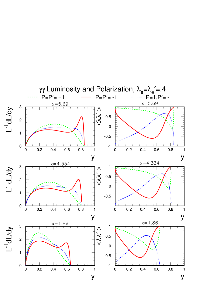
Figure 1: The normalized differential luminosity ${1\over{\cal L}_{\gamma\gamma}}{d{\cal L}_{\gamma\gamma}\over dy}$ and the corresponding $\langle\lambda\lambda^{\prime}\rangle$ for $\lambda_{e}=\lambda^{\prime}_{e}=.4$ (80% polarization) and three different choices of the initial laser photon polarizations $P$ and $P^{\prime}$. The distributions shown are for $\rho^{2}\ll 1$ [17, 18]. Results for $x=5.69$, $x=4.334$ and $x=1.86$ are compared.

The computation of $d{\cal L}_{\gamma\gamma}/dy$ was first considered in [17, 18]. We review results based on their formulae assuming $\rho^{2}\ll 1$, where $\rho$ characterizes the distance from the electron laser collision to the $\gamma\gamma$ interaction point. (See [17, 18]. When $\rho$ is substantial in size, the low $E_{\gamma\gamma}$ part of the spectrum predicted by their formulae is suppressed. However, beamstrahlung greatly enhances the luminosity in this region, as we shall discuss.) There are three independent choices for $\lambda_{e}$, $\lambda^{\prime}_{e}$, $P$ and $P^{\prime}$. Assuming 80% polarization is possible for the $e$ beams, the values of $F(y)={1\over{\cal L}_{\gamma\gamma}}{d{\cal L}_{\gamma\gamma}\over dy}$ and $\langle\lambda\lambda^{\prime}\rangle$ are plotted as a function of $y$ in Fig. 1 for the three independent choices of relative electron and laser polarization orientations, and for $x=5.69$, $x=4.334$ and $x=1.86$. (The relevance of these particular $x$ values will emerge very shortly). We observe that the choice (I) of $\lambda_{e}=\lambda^{\prime}_{e}=.4$, $P=P^{\prime}=1$ gives large $\langle\lambda\lambda^{\prime}\rangle$ and $F(y)>1$ for small to moderate $y$. The choice (II) of $\lambda_{e}=\lambda^{\prime}_{e}=.4$, $P=P^{\prime}=-1$ yields a peaked spectrum with $\langle\lambda\lambda^{\prime}\rangle>0.85$ at the peak. Finally, the choice (III) of $\lambda_{e}=\lambda^{\prime}_{e}=.4$, $P=1,P^{\prime}=-1$ gives a broad spectrum, but never achieves large $\langle\lambda\lambda^{\prime}\rangle$. As earlier noted, large values of $\langle\lambda\lambda^{\prime}\rangle$ are important for suppressing the $b\overline{b}$ continuum Higgs detection background, with leading tree-level term $\propto 1-\langle\lambda\lambda^{\prime}\rangle$. Thus, the peaked spectrum choice (II) is most suited to Higgs studies. In fact, because $\langle\lambda\lambda^{\prime}\rangle$ increases rapidly as $y$ increases just past the peak location, it is always possible to find a value of $y$ for which $F(y)\sim 95\%$ of its peak value while $\langle\lambda\lambda^{\prime}\rangle\sim 0.9$. A final important point is to note that it is really very important for both $e$ beams to be polarized in order to minimize the $1-\langle\lambda\lambda^{\prime}\rangle$ component of the background and that luminosity and polarization at the peak are very significantly reduced if one beam is unpolarized. Current technology only allows for large $e^{-}$ polarization at high luminosity. Unless techniques for achieving large $e^{+}$ polarization at high luminosity are developed [19], Higgs studies at a $\gamma\gamma$ collider demand $e^{-}e^{-}$ collisions. Thus, it may be very difficult to perform Higgs studies at a 2nd ‘parasitic’ interaction region during $e^{+}e^{-}$ operation.

Let us now turn to the relevance of the particular $x$ values illustrated in Fig. 1. If the laser energy is adjustable, $x\sim 4.8$ is often deemed to be an optimal choice (yielding $y_{\rm max}\sim 0.82$) in that it is the largest value consistent with being below the pair creation threshold, while at the same time it maximizes the peak structure (at $y\sim 0.8$) for the case (II) spectrum. More realistically, however, the fundamental laser wavelength will be fixed; the Livermore group has determined that a wavelength of 1.054 microns is the most technologically feasible value — see Section 5 of Chapter 13, p. 359-366 of Ref. [3]. The subpulse energy of the Livermore design is 1 Joule. This results in a probability of $\sim 65\%$ that a given electron in one bunch will interact with a photon. Higher values for the subpulse energy are possible, but would result in more multiple interactions and increased non-linear effects. The subpulse energy chosen is felt to be a good compromise value for achieving good luminosity without being overwhelmed by such effects.

For a fixed wavelength, $x$ will vary as the machine energy is varied. For a wavelength of $\lambda=1.054~{}\mu$, representative values are $x=1.86$ at a machine energy of $\sqrt{s}=206~{}{\rm GeV}$, for which $P\lambda_{e}<0,P^{\prime}\lambda_{e}^{\prime}<0$ yields a spectrum peaking at $E_{\gamma\gamma}\sim 120~{}{\rm GeV}$ (as appropriate for a light Higgs boson), and $x=5.69$ at $\sqrt{s}=630~{}{\rm GeV}$, for which $P\lambda_{e}<0,P^{\prime}\lambda_{e}^{\prime}<0$ yields a spectrum peaking at $E_{\gamma\gamma}\sim 500~{}{\rm GeV}$ (as appropriate for a heavy Higgs boson). However, as illustrated in Fig. 1, the peaking for $x=1.86$ is not very strong as compared to higher $x$ values. Further, the value of $1-\langle\lambda\lambda^{\prime}\rangle$ at the peak (to which backgrounds for Higgs detection are proportional) for $x=1.86$ is somewhat larger than for large $x$ values. Fortunately, the Livermore group has developed a technique by which the laser frequency can be tripled. In this way, the $x$ value can be tripled for a given $\sqrt{s}$, allowing for a much more peaked spectrum, and smaller $1-\langle\lambda\lambda^{\prime}\rangle$ at the peak, for the light Higgs case. For $\lambda\sim 1/3~{}\mu$, a spectrum peaked at $E_{\gamma\gamma}=120~{}{\rm GeV}$ is obtained by operating at $\sqrt{s}=160~{}{\rm GeV}$, yielding $x=4.334$. The spectra for this case is also plotted in Fig. 1. The much improved peaking for $x=4.334$ as compared to $x=1.86$ is apparent. Regarding $x=5.69$, it has been argued in the past that $x>4.8$ is undesirable in that it leads to pair creation. However, our studies, which include these effects, indicate that the resulting backgrounds are not a problem.

We will return to the importance of including the full dependence of the acceptance on $z$ and $z^{\prime}$ shortly. For now, let us continue to neglect this dependence and review a few more of the ‘standard’ results.

3 Realistic $E_{\gamma\gamma}$ spectra

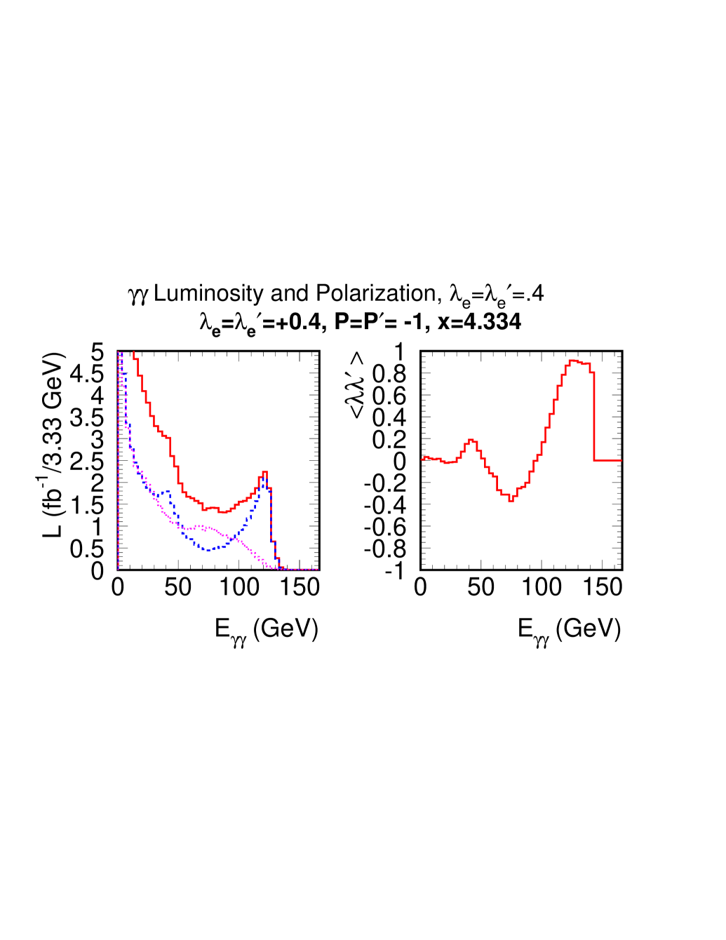
Figure 2: We plot the CAIN [20] predictions for the $\gamma\gamma$ luminosity, $L=d{\cal L}/dE_{\gamma\gamma}$, in units of $~{}{\rm fb}^{-1}/3.33~{}{\rm GeV}$ (3.33 GeV being the bin size) for circularly polarized [case (II)] photons assuming a $10^{7}$ sec year, $\sqrt{s}=160~{}{\rm GeV}$, 80% electron beam polarization, and a 1.054/3 micron laser wave length. Beamstrahlung and other effects are included. The dashed (dotted) curve gives the component of the total luminosity that derives from the $J_{z}=0$ ($J_{z}=2$) two-photon configuration. Also plotted is the corresponding value of $\langle\lambda\lambda^{\prime}\rangle$ [given by $\langle\lambda\lambda^{\prime}\rangle=(L_{J_{z}=0}-L_{J_{z}=2})/(L_{J_{z}=0}+L_{J_{z}=2})$].

There are important corrections to the naive luminosity distributions just considered. First, the luminosity at low $E_{\gamma\gamma}$ is affected by two conflicting corrections. Finite $\rho$ suppresses the low-$E_{\gamma\gamma}$ luminosity. However, this effect is more than compensated by beamstrahlung, secondary collisions between scattered electrons and photons from the laser beam and other non-linear effects. The result is a substantial enhancement of the luminosity in the low-$E_{\gamma\gamma}$ region. This is illustrated in Fig. 2 for case (II) polarization orientation choices and for $\sqrt{s}=160~{}{\rm GeV}$, which yields $x=4.33$ for a 1.054 micron laser source running with the ‘frequency tripler’, and a (CP-IP) separation between the photon conversion point (CP) and photon-photon interaction point (IP) of 1 mm. We also note that all the spectra considered here were obtained for flat electron beams. (For a given CP-IP separation, round electron beams would give a factor of roughly two larger luminosity. However, we chose the flat beam configuration for consistency with the final-focus and collimation arrangements that will be used in $e^{+}e^{-}$ collisions.) As expected from Fig. 1, the spectrum shows a peak at $E_{\gamma\gamma}=120~{}{\rm GeV}$ (as might correspond to a light Higgs boson mass). However, the low-$E_{\gamma\gamma}$ tail is now quite substantial. This implies that it will be very important to achieve a small mass resolution, $\Gamma_{\rm res}$, for the final state reconstruction. The luminosity $\Delta{\cal L}_{\gamma\gamma}$ in the bin centered at $E_{\gamma\gamma}=120~{}{\rm GeV}$ is equivalent to $d{\cal L}/dE_{\gamma\gamma}\sim 0.66~{}{\rm fb}^{-1}/~{}{\rm GeV}$ per $10^{7}$ sec year. The corresponding luminosity at TESLA could be as much as a factor of 2 larger due to higher repetition rate and larger charge per bunch. If one wishes to avoid a large low-$E_{\gamma\gamma}$ tail, then it is necessary to have a significantly different configuration, including much larger CP-IP separation and/or a high-field sweeping magnet. These options were considered (also using the CAIN program) in the Asian Committee for Future Accelerators (ACFA) report [4], where a CP-IP separation of 1 cm was adopted and a 3 Tesla sweeping magnet was employed.  The disadvantage of this arrangement is a substantially lower value for $d{\cal L}/dE_{\gamma\gamma}$ at the peak, at least for the corresponding bunch charge, repetition rate and spot size employed in [4]. As noted above, we have $d{\cal L}/dE_{\gamma\gamma}\sim 0.66~{}{\rm fb}^{-1}/~{}{\rm GeV}$ per year, which should be compared to $\sim 0.13~{}{\rm fb}^{-1}/~{}{\rm GeV}$ per year for the ACFA report choices. The latter leads to a much larger error for the precision studies of a light SM-like Higgs boson (despite the assumption of 100% polarization for the $e$ beams). In the TESLA Technical Design Report (TDR) [6], a CP-IP separation of 2.1 mm (2.7 mm) is used for $\sqrt{s}=500~{}{\rm GeV}$ ($\sqrt{s}=800~{}{\rm GeV}$). A flat beam configuration is employed. Combining information from Fig. 1.4.7 and Table 1.4.1 ($200~{}{\rm GeV}$ numbers) in Part VI (Appendices) of the TESLA TDR [6], we estimate that the TESLA design will give $d{\cal L}/dE_{\gamma\gamma}\sim 1.8~{}{\rm fb}^{-1}/~{}{\rm GeV}$ per year, more than a factor of 2 better  than our $\sim 0.66~{}{\rm fb}^{-1}/~{}{\rm GeV}$ that we shall employ for studying a Higgs with mass of $120~{}{\rm GeV}$.

Turning to the important average $\langle\lambda\lambda^{\prime}\rangle$, we note that the naively predicted value for $\langle\lambda\lambda^{\prime}\rangle$ at the luminosity peak is about 0.86 (see Fig. 1), rising rapidly to higher values as $y$ increases. For instance, $\langle\lambda\lambda^{\prime}\rangle\sim 0.96$ at the point where the luminosity has fallen only 25% from its peak value. From Fig. 2 we see that the CAIN Monte Carlo predicts that this behavior of $\langle\lambda\lambda^{\prime}\rangle$ is smoothed out somewhat after including the beamstrahlung contribution, but the value at the luminosity peak of $\langle\lambda\lambda^{\prime}\rangle\sim 0.85$ is nearly the same as predicted in the naive case. 

The above results are still somewhat misleading due to the fact that we have not yet incorporated the dependence of the acceptance function $A(z,z^{\prime},z_{\theta^{*}})$. For the Higgs signal that is independent of $z_{\theta^{*}}$, it is useful to define

$${\textstyle{1\over 2}}\sum_{\lambda,\lambda^{\prime}}\int dzdz^{\prime}\int dz_{\theta^{*}}{d{\cal L}_{\gamma}^{\lambda}(\lambda_{e},P,z)\over dz}{d{\cal L}_{\gamma}^{\lambda^{\prime}}(\lambda_{e}^{\prime},P^{\prime},z^{\prime})\over dz^{\prime}}A(z,z^{\prime},z_{\theta^{*}})[1,\lambda\lambda^{\prime}]$$

$$\equiv\int dy{d{\cal L}_{\gamma\gamma}^{\rm eff}(\lambda_{e},\lambda_{e}^{\prime},P,P^{\prime},y)\over dy}[1,\langle\lambda\lambda^{\prime}\rangle^{\rm eff}(y)]\,,$$ (7)

yielding

$$N(\gamma\gamma\to{h}\to X) = {4\pi^{2}\Gamma({h}\to\gamma\gamma)BR({h}\to X)(1+\langle\lambda\lambda^{\prime}\rangle^{\rm eff}(y))\over\sqrt{s}m_{h}^{2}}\left.{d{\cal L}_{\gamma\gamma}^{\rm eff}\over dy}\right|_{y=m_{h}/\sqrt{s}}\,.$$ (8)

The effective luminosity and $\langle\lambda\lambda^{\prime}\rangle$ depends on the cut $|z_{\theta^{*}}|<0.5$ and the standard LC detector acceptances, including, in particular, the requirement that the jets pass fully through the vertex detector and be fully reconstructed (with little energy in the uninstrumented forward and backward regions). For $E_{\gamma\gamma}$ substantially below the peak region, the peak being in the vicinity of $E_{\gamma\gamma}\sim 120~{}{\rm GeV}$, the effective luminosity for Higgs production is only slightly suppressed (beyond the obvious factor of 0.5 coming from the $|z_{\theta^{*}}|<0.5$ cuts).

4 Studying a light SM-like Higgs boson

Consider first a SM-like Higgs boson $h$ of relatively light mass; SM-like Higgs bosons arise in many models containing physics beyond the SM. The $h\to\gamma\gamma$ coupling receives contributions from loops containing any charged particle whose mass, $M$, arises in whole or part from the vacuum expectation value of the corresponding neutral Higgs field. (Of course, in the strict context of the SM, the masses of all elementary particles derive entirely from the Higgs field vacuum expectation value.) When the mass, $M$, derives in whole or part from the vacuum expectation value ($v$) of the neutral Higgs field associated with the $h$, then in the limit of $M\gg m_{h}$ for the particle in the loop, the contribution asymptotes to a value that depends on the particle’s spin (i.e. the contribution does not decouple). As a result, a measurement of $\Gamma(h\to\gamma\gamma)$ provides the possibility of revealing the presence of heavy charged particles that acquire their mass via the Higgs mechanism. Of course, since the mass deriving from the SM-like neutral Higgs vev $v$ is basically proportional to some coupling times $v$, if the coupling is perturbative the mass of the heavy particle is unlikely to be much larger than $0.5-1$ TeV. In addition, we note that $BR(h\to X)$ is entirely determined by the spectrum of particles with mass $<m_{h}/2$, and is not affected by heavy states with $M>m_{h}/2$. Consequently, measuring $N(\gamma\gamma\to h\to X)$ provides an excellent probe of new heavy particles with mass deriving from the Higgs mechanism. We emphasize that in models beyond the SM, particles can acquire mass from mechanisms other than the Higgs mechanism. If there is a SM-like Higgs boson in such an extended model the loop contributions from the charged particles that acquire a large mass from some such alternative mechanism will decouple as $({\rm mass})^{-2}$ and $\gamma\gamma\to h$ will not be sensitive to their presence.

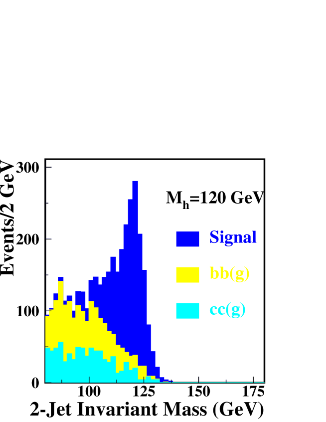
Figure 3: Higgs signal and heavy quark backgrounds in units of events per 2 GeV for a Higgs mass of 120 GeV and assuming a running year of $10^{7}$ sec. We have employed the cuts as given in the text.

If there are no new particles that acquire mass via the Higgs mechanism, a precision measurement of $\Gamma({\widehat{h}}\to\gamma\gamma)$ can allow one to distinguish between a ${\widehat{h}}$ that is part of a larger Higgs sector and the SM $h_{SM}$. Fig. 3 shows the di-jet invariant mass distributions for the $m_{h_{SM}}=120~{}{\rm GeV}$ Higgs signal and for the $b\overline{b}(g)$ and $c\overline{c}(g)$ backgrounds, using the luminosity distribution of Fig. 2, after all cuts. Our analysis is similar, but not identical, to that of Ref. [21]. See also [22, 23, 9, 10]. Both employ JETSET fragmentation using the Durham algorithm choice of $y_{\rm cut}=0.02$ for defining the jets. Further, we employ the event mixture predicted by PYTHIA (passed through JETSET) [24] and we use the LC Fast Monte Carlo detector simulation within ROOT [25], which includes calorimeter smearing and detector configuration as described in Section 4.1 of Chapter 15 of Ref. [3]. The signal is generated using PANDORA plus PYTHIA/JETSET [26]. We have employed the following cuts.

• Only tracks and showers with $|\cos\theta|<0.9$ in the laboratory frame are accepted.

• Tracks are required to have momentum greater than 200 MeV and showers must have energy greater than 100 MeV.

• We then focus on the two most energetic jets in the event (with jets defined using $y_{\rm cut}=0.02$).

• We require these two jets to be back-to-back in three dimensions using the criteria $|p_{i}^{1}+p_{i}^{2}|<12~{}{\rm GeV}$ for $i=x,y,z$.

• We require $|\cos\theta^{*}|<0.5$, where $\theta^{*}$ is the angle of the two most energetic jets in their center of mass relative to the beam direction. The alternative of $|\cos\theta|<0.5$ results in very little change for $E_{\gamma\gamma}>80~{}{\rm GeV}$ once the preceding back-to-back cut has been applied.

We note that even though we do not explicitly require exactly two-jets in the final state, the third and fourth cuts listed above, especially the back-to-back requirement, results in 90% of the retained events containing exactly two jets.

We employ the two most energetic jets (after imposing the cuts given above) to reconstruct the Higgs boson signal. Our mass resolution for the narrow-width Higgs boson signal is $4.76\pm 0.13~{}{\rm GeV}$ (for a Gaussian fit from $-1\sigma$ to $+10\sigma$) which is similar to the $\sim 6~{}{\rm GeV}$ found in [21]. We believe that the difference in mass resolution is due primarily to differences in the Monte Carlo’s employed. If we keep only events with $M_{2~{}\rm jet}\geq 110~{}{\rm GeV}$, there are roughly 1450 signal events and about 335 background events, after all cuts. This would yield a measurement of $\Gamma(h_{SM}\to\gamma\gamma)BR(h_{SM}\to b\overline{b})$ with an accuracy of $\sqrt{S+B}/S\sim 2.9\%$.  The error for this measurement increases to about $10\%$ for $m_{h_{SM}}\sim 160~{}{\rm GeV}$ given the predicted signal rate, $S:B\sim 1:1$ and $\langle\lambda\lambda^{\prime}\rangle\sim 0.85$ at the peak. These accuracies are those estimated for one $10^{7}$ sec year of operation. Deviations due to ${\widehat{h}}\neq h_{SM}$ in an extended Higgs sector model typically exceed 3% if the other heavier Higgs bosons have masses below about 500 GeV (so that there are significant corrections to the decoupling limit). To obtain the above results, excellent $b$ tagging is essential to eliminate backgrounds from light quark states. We have not simulated $b$-tagging. Rather we have assumed (as in [21]) 70% efficiency for double-tagging $b\overline{b}$ events (after having already made the necessary kinematic cuts), for which there is a 3.5% efficiency for tagging $c\overline{c}$ events as $b\overline{b}$, a rejection factor of 20. This rejection factor is very essential since, crudely speaking, the $c\overline{c}$ background is a factor of 16 ($=(q_{c}/q_{b})^{4}$) larger without this rejection. After including the tagging rejection, the $c\overline{c}$ and $b\overline{b}$ backgrounds are roughly comparable.

We should note explicitly that we have performed our background and signal cross section calculations at tree-level. Various studies have appeared in the literature showing that under some circumstances higher order corrections and other effects can be quite important. We have explicitly chosen our cuts so that they are not. In particular, we have employed cuts that primarily retain only events with two jets. It is the processes with extra radiated gluons (which are included as part of the NLO radiative corrections) that can cause the largest corrections since the associated cross sections are not proportional to $1-\langle\lambda\lambda^{\prime}\rangle$. As discussed in more detail in Appendix B, NLO corrections to two-jet events, while sizable, will not significantly impact our results. The primary reason for employing tree-level computations is the importance of being able to perform full simulation analyzes, something that is only possible in the context of PANDORA and JETSET for the signal and in the context of PYTHIA and JETSET for the background. We estimate our errors are not more than 10%-20% as a result of ignoring higher order corrections. Appendix B is devoted to a more detailed discussion of the relevant issues.

5 The $H^{0}$ and $A^{0}$ of the MSSM

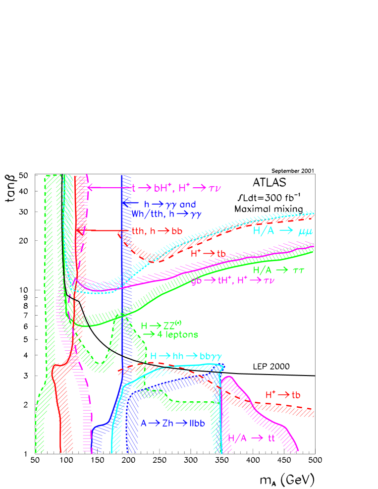
Figure 4: $5\sigma$ discovery contours for MSSM Higgs boson detection in various channels are shown in the $[m_{A^{0}},\tan\beta]$ parameter plane, assuming maximal mixing and an integrated luminosity of $L=300~{}{\rm fb}^{-1}$ for the ATLAS detector. This figure is preliminary [27].

In many scenarios, it is very possible that by combining results from $\gamma\gamma\to h^{0}\to b\overline{b}$ with other types of precision measurements for the SM-like Higgs boson, we will observe small deviations and suspect the presence of heavy Higgs bosons. Giga-$Z$  precision measurements could provide additional indirect evidence for extra Higgs bosons through a very precise determination of the $S$ and $T$ parameters, which receive corrections from loops involving the extra Higgs bosons. However, to directly produce the heavier Higgs in $e^{+}e^{-}$ collisions is likely to require large machine energy. For example, In the 2HDM $e^{+}e^{-}\to H^{0}A^{0}$ pair production would be the most relevant process in the decoupling limit, but requires $\sqrt{s}>m_{H^{0}}+m_{A^{0}}$, with $m_{H^{0}}+m_{A^{0}}\sim 2m_{A^{0}}$ as the decoupling limit sets in. The alternatives of $b\overline{b}H^{0}$ and $b\overline{b}A^{0}$ production will only allow $H^{0}$ and $A^{0}$ detection if $\tan\beta$ is large [8]. Either low or high $\tan\beta$ is also required for LHC discovery of the $H^{0},A^{0}$ if they have mass $\mathrel{\raise 1.29167pt\hbox{$>$\kern-7.5pt\lower 4.30554pt\hbox{$\sim$}}}250~{}{\rm GeV}$. This is illustrated in Fig. 4. After accumulation of $L=300~{}{\rm fb}^{-1}$ at the LHC, the $H^{0},A^{0}$ will be detected except in the wedge of parameter space with $m_{A^{0}}\mathrel{\raise 1.29167pt\hbox{$>$\kern-7.5pt\lower 4.30554pt\hbox{$\sim$}}}250~{}{\rm GeV}$ and moderate $\tan\beta$ (where only the $h^{0}$ can be detected). If the LC is operated at $\sqrt{s}=630~{}{\rm GeV}$, then detection of $e^{+}e^{-}\to H^{0}A^{0}$ will be possible for $m_{A^{0}}\sim m_{H^{0}}$ up to nearly 300 GeV. In this case, the parameter region for which some other means of detecting the $H^{0},A^{0}$ must be found is the portion of the LHC wedge with $m_{A^{0}}\mathrel{\raise 1.29167pt\hbox{$>$\kern-7.5pt\lower 4.30554pt\hbox{$\sim$}}}300~{}{\rm GeV}$. We will explore the possibility of finding the $H^{0}$ and $A^{0}$ in $\gamma\gamma$ collisions. Earlier work along this line appears in [9, 10]. Our results will incorporate CAIN predictions for the luminosity and polarizations of the colliding back-scattered photons using 80% polarization for the electron beams (which we believe is more realistic than the 100% polarization assumed in [9, 10]).

We will show that single $H^{0},A^{0}$ production via $\gamma\gamma$ collisions will allow their discovery throughout a large fraction of this wedge. The event rate, see Eq. (6), can be substantial due to quark loop contributions (mainly $t$ and, at high $\tan\beta$, $b$) and loops containing other new particles (e.g. the charginos, $\ldots$ of supersymmetry). In this study, we will also assume that the superparticle masses (for the charginos, squarks, sleptons, etc..) are sufficiently heavy that (a) the Higgs bosons do not decay to superparticles and (b) the superparticle loop contributions to the $\gamma\gamma$ coupling are negligible.

Assuming no reliable preconstraints on $m_{A^{0}},m_{H^{0}}$, an important question is whether it is best to search for the $H^{0},A^{0}$ by scanning in $\sqrt{s}$ (and thereby in $E_{\gamma\gamma}$, assuming type-II peaked spectrum configuration) or running at fixed $\sqrt{s}$ using a broad $E_{\gamma\gamma}$ spectrum part of the time and a peaked spectrum the rest of the time [1]. As we shall discuss, if covering the wedge region is the goal, then running at a single energy, part of the time with a peaked $E_{\gamma\gamma}$ luminosity distribution and part of the time with a broad distribution (in ratio 2:1), would be a somewhat preferable approach.

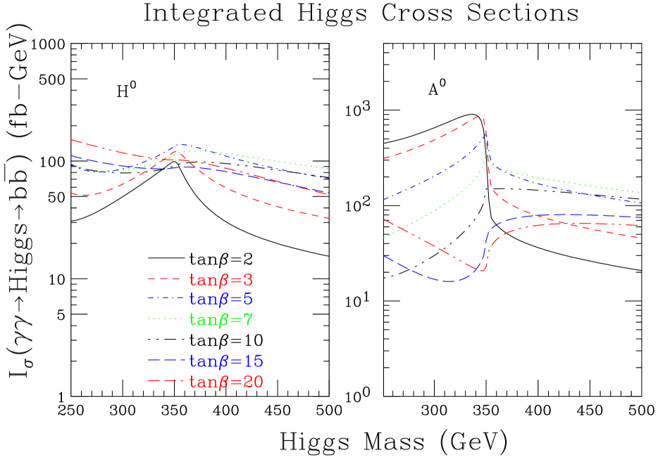
Figure 5: We plot the integrated $H^{0}$ and $A^{0}$ Higgs cross sections $I_{\sigma}$, as defined in Eq. (6), as a function of Higgs mass, for a variety of $\tan\beta$ values. We employ the maximal-mixing scenario with $m_{\rm SUSY}=1~{}{\rm TeV}$. Supersymmetric particle loops are neglected.

The first important input to the calculations is the effective integrated cross section, $I_{\sigma}$, as defined in Eq. (6), for the $H^{0}$ and $A^{0}$. These cross sections are plotted as a function of Higgs mass for a variety of $\tan\beta$ values in Fig. 5. We have computed the cross sections using the $b\overline{b}$ branching ratios and $\gamma\gamma$ widths obtained from HDECAY [28] using input masses of $m_{A^{0}}$ as plotted on the $x$-axes. We have employed $m_{t}=175~{}{\rm GeV}$, exactly. For Supersymmetry (SUSY) parameters, we have chosen $m_{\rm SUSY}=1~{}{\rm TeV}$ for all slepton and squark soft-SUSY-breaking masses and $\mu=+1~{}{\rm TeV}$. For $A_{t}$ we have assumed the maximal-mixing choice of $A_{t}=\mu/\tan\beta+\sqrt{6}m_{\rm SUSY}$. In addition, we have taken $A_{b}=A_{\tau}=A_{t}$. Our plots have been restricted to $m_{A^{0}}\leq 500~{}{\rm GeV}$ due to the fact that if the LC is operated at $\sqrt{s}=630~{}{\rm GeV}$ (corresponding to $x\sim 5.69$ for 1 micron laser wavelength) we can potentially probe Higgs masses as high as $\sim 500~{}{\rm GeV}$.

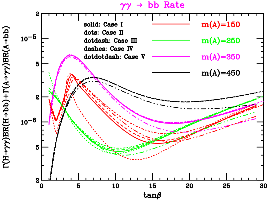
Figure 6: We plot the sum $\Gamma(H^{0}\to\gamma\gamma)BR(H^{0}\to b\overline{b})+\Gamma(A^{0}\to\gamma\gamma)BR(A^{0}\to b\overline{b})$ as a function of $\tan\beta$ for several $m_{A^{0}}$ values. The signal rate $N(\gamma\gamma\to H^{0},A^{0}\to b\overline{b})$ is roughly proportional to this quantity. Results for the five cases delineated in the text are shown.

An interesting question is the extent to which these inputs are model dependent in that they are sensitive to other parameters of the MSSM. Our study has been performed for the maximal-mixing scenario with $m_{t}=175~{}{\rm GeV}$ and $m_{\rm SUSY}=1~{}{\rm TeV}$, assuming that all SUSY particles are heavy enough to not significantly influence the $\gamma\gamma\to H^{0},A^{0}$ couplings and heavy enough that $H^{0},A^{0}\to$ SUSY decays are not significant. (In the context of HDECAY, we have set IOFSUSY=1.) If SUSY particles are moderately light, there will be some, but not dramatic modifications to the couplings and some dilution of the $H^{0},A^{0}\to b\overline{b}$ branching ratios. These effects will be minimal at the higher $\tan\beta$ values in the wedge region, but could make discovery in the $b\overline{b}$ channel difficult for some of the lower $\tan\beta$ points. One would undoubtedly try to make use of the SUSY decay channels themselves to enhance the net signal for $\gamma\gamma\to H^{0},A^{0}$. Even if SUSY particles are all heavy, there could be some variation as one moves from the maximal-mixing scenario to the no-mixing scenario, and so forth. Further, there are certain non-decoupling loop corrections to the relation between $m_{b}$ and the $H^{0},A^{0}\to b\overline{b}$ Yukawa couplings that could either enhance or diminish the $\gamma\gamma\to H^{0},A^{0}\to b\overline{b}$ rates [29]. (These are not currently incorporated into the standard version of HDECAY.) We have performed a limited exploration by considering five cases. Computations for cases I-IV are performed using version 2.0 of HDECAY, i.e. that available as of September 2001.

I: The maximal-mixing scenario defined above.

II: The maximal-mixing scenario as above, but with $\mu=-1~{}{\rm TeV}$.

III: The no-mixing scenario defined by $A_{b}=A_{\tau}=A_{t}=\mu/\tan\beta$, with $m_{\rm SUSY}=\mu=1~{}{\rm TeV}$.

IV: The maximal-mixing scenario, as in case I, but with $\mu=0$.

V: In this case, we employ the maximal mixing scenario with $m_{\rm SUSY}=\mu=1~{}{\rm TeV}$, but employ a modified version of HDECAY (provided by the authors of Ref. [29]) in which the $\Delta\lambda_{b}$ corrections to the Higgs $b\overline{b}$ vertices are included. These arise from loop corrections involving supersymmetric particles (neglected in cases I-IV), and are most substantial when $\tan\beta$ is large. These corrections do not vanish (i.e. do not decouple) even when SUSY particle masses are large. The corrections would have opposite sign to those plotted for $\mu=-1~{}{\rm TeV}$.

The results in each of the above five cases for $\Gamma(H^{0}\to\gamma\gamma)BR(H^{0}\to b\overline{b})+\Gamma(A^{0}\to\gamma\gamma)BR(A^{0}\to b\overline{b})$ (to which the signal rate $N(\gamma\gamma\to H^{0},A^{0}\to b\overline{b})$ is roughly proportional) are plotted in Fig. 6 as a function of $\tan\beta$ for several $m_{A^{0}}$ values. We observe that, although there is considerable model dependence for the relatively low mass of $m_{A^{0}}=150~{}{\rm GeV}$, this model dependence becomes quite minimal when comparing cases I-IV for $m_{A^{0}}\geq 250~{}{\rm GeV}$, i.e. in the wedge region of interest. However, results for case V show that SUSY loop corrections can impact the predicted signal event rate once $\tan\beta$ is large enough, but remains minimal for $m_{A^{0}}\leq 500~{}{\rm GeV}$ and $\tan\beta$ values in the wedge region.

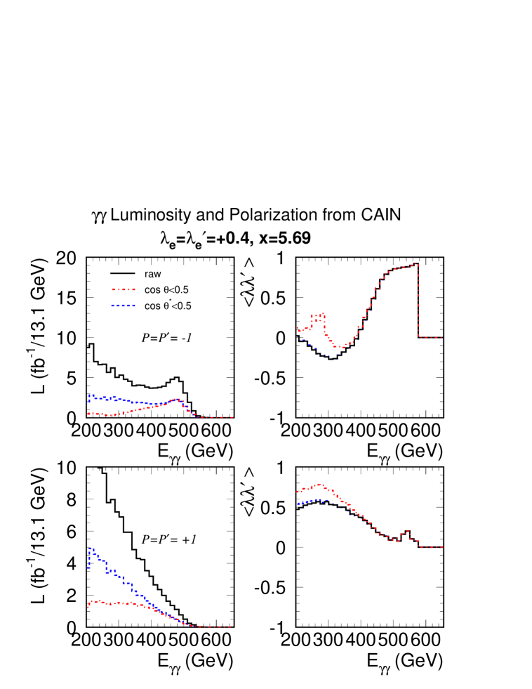
Figure 7: Luminosity, in units $~{}{\rm fb}^{-1}/13.1~{}{\rm GeV}$, for a $10^{7}$ sec year and associated $\langle\lambda\lambda^{\prime}\rangle$ are plotted for $\sqrt{s}=630~{}{\rm GeV}$ ($x=5.69$ for $1.054~{}\mu$m laser wavelength), assuming 80% electron beam polarizations, for polarization orientation cases (I) and (II). Results are plotted for 3 different cases. The solid lines show the results before any cuts or reconstruction efficiencies are incorporated. The dashed and dash-dot lines assume that the two most energetic jets are produced uniformly (as for a spin-0 boson decaying to two jets) in $\cos\theta^{*}$, where $\theta^{*}$ is the two-jet axis angle relative to the beam direction in the two-jet rest frame. The dashed lines show the results after requiring $|\cos\theta^{*}|<0.5$. The dash-dot lines show the results after requiring $|\cos\theta|<0.5$ for the $\theta$’s of the two most energetic jets in the laboratory rest frame.

The next important inputs are values of ${d{\cal L}\over dE_{\gamma\gamma}}$ and $\langle\lambda\lambda^{\prime}\rangle$ for the peaked spectrum (type-II) and broad spectrum (type-I) electron-laser-photon polarization configurations. The luminosity and polarization results from the CAIN [20] Monte Carlo program are plotted as the solid curves in Fig. 7. Note again the luminosity enhancement at low $E_{\gamma\gamma}$ relative to naive expectations. In the case of the type-II spectrum, the luminosity remains quite large even below the $E_{\gamma\gamma}$ peak at $E_{\gamma\gamma}=500~{}{\rm GeV}$, and that $\langle\lambda\lambda^{\prime}\rangle$ is large for $E_{\gamma\gamma}>450~{}{\rm GeV}$. In the case of the type-I spectrum, the luminosity grows is substantial for $E_{\gamma\gamma}=400~{}{\rm GeV}$ and rises rapidly with decreasing $E_{\gamma\gamma}$. In addition, reasonably large $\langle\lambda\lambda^{\prime}\rangle$ is retained for $250<E_{\gamma\gamma}<400~{}{\rm GeV}$. However, in both cases, the values of $\langle\lambda\lambda^{\prime}\rangle$ are always small enough that the $J_{z}=2$ part of the $b\overline{b}$ background to Higgs detection will be only partially suppressed by the $1-\langle\lambda\lambda^{\prime}\rangle$ factor, and will be dominant.

The final ingredient is to assess the impact of the cuts required to reduce the $b\overline{b}(g)$ and $c\overline{c}(g)$ backgrounds to an acceptable level. In order to access the Higgs bosons with mass substantially below the machine energy of 630 GeV, we must employ cuts that remove as little luminosity for $E_{\gamma\gamma}$ substantially below $\sqrt{s}$ as possible while still eliminating most of the background. For this purpose, a cut on $|\cos\theta^{*}|<0.5$ (where $\theta^{*}$ is the angle of the two most energetic jets relative to the beam direction in the two-jet rest frame) is far more optimal than is a cut of $|\cos\theta|<0.5$ (where $\theta$ is the angle of a jet in the laboratory frame). This is illustrated in Fig. 7 where it is seen that the former cut on $\theta^{*}$ leads to much higher luminosity than the latter cut on $\theta$. Thus, even though slightly larger $\langle\lambda\lambda^{\prime}\rangle$ is obtained using the $\theta$ cuts, much better signals (relative to background) are achieved using the $\theta^{*}$ cut. A second cut is that imposed upon the two-jet mass distribution. The optimal value for this cut depends upon the Higgs widths, the degree of degeneracy of the $H^{0}$ and $A^{0}$ masses, and the detector resolutions and reconstruction techniques.

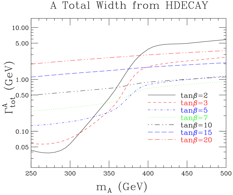
Figure 8: We plot the total width of the $A^{0}$ as a function of $m_{A^{0}}$ for our standard set of $\tan\beta$ values. Results are those from HDECAY for the earlier defined maximal mixing scenario with $m_{\rm SUSY}=\mu=1~{}{\rm TeV}$. Supersymmetric particle loops are neglected.

Figure 8 shows the total $A^{0}$ width as a function for $m_{A^{0}}$ for our standard set of $\tan\beta$ values. For the $\tan\beta$ range inside the problematical wedge ($15>\tan\beta>3$), the $A^{0}$ (and also the $H^{0}$) is still relatively narrow, with widths below $\sim 3$ GeV. In fact, the width of the two-jet mass distribution will probably derive mostly from detector resolutions and reconstruction procedures. A full Monte Carlo analysis for heavy Higgs bosons with relatively small widths is not yet available. However, there are many claims in the literature that the resulting mass resolution will almost certainly be better than $\Delta m_{\rm 2-jet}=30\%\sqrt{m_{\rm 2-jet}}$ (the result obtained assuming $\Delta E_{\rm jet}=18\%\sqrt{E_{\rm jet}}$ for each of the back-to-back jets) [3, 4, 5, 6]. Very roughly this corresponds to a full-width at half maximum of about $6~{}{\rm GeV}$ in the mass range from $250-500~{}{\rm GeV}$ of interest.

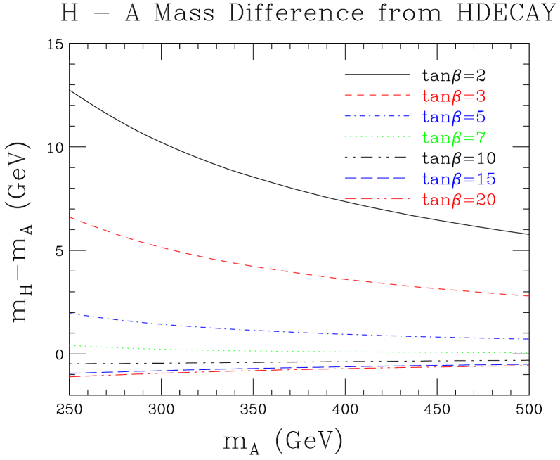
Figure 9: We plot difference $m_{H^{0}}-m_{A^{0}}$ as a function of $m_{A^{0}}$ for our standard set of $\tan\beta$ values. Results are those from HDECAY for the earlier defined maximal mixing scenario with $m_{\rm SUSY}=\mu=1~{}{\rm TeV}$. Supersymmetric particle loops are neglected.

The second important ingredient in understanding the nature of $H^{0},A^{0}$ signal is the degree to which they are degenerate in mass. The degree of non-degeneracy is plotted in Fig. 9. For $\tan\beta=2$ and 3, the mass differences at lower $m_{A^{0}}$ are such that the $H^{0}$ and $A^{0}$ peaks would remain substantially separated even after including $\sim 6~{}{\rm GeV}$ experimental mass resolution. However, starting with $\tan\beta=5$, and for larger $m_{A^{0}}>2m_{t}$ in the $\tan\beta=2,3$ cases, the mass difference is sufficiently small and their total widths sufficiently large that after including experimental mass resolution there will be considerable overlap between the $H^{0}$ and $A^{0}$ peaks. A centrally located 10 GeV bin would pick up a large fraction of the $H^{0}$ and $A^{0}$ events.. The assumption that 50% of the total number of $H^{0}$ and $A^{0}$ events fall into one 10 GeV bin centered on $m_{A^{0}}$ is thus an approximate way of taking into account both the $6~{}{\rm GeV}$ experimental mass resolution, the few GeV total widths and the non-degeneracy. While 50% is probably an overestimate for $\tan\beta=2,3$ and lower $m_{A^{0}}$, it is not much of an overestimate because, for these parameter cases, the $A^{0}$ signal is much stronger than the $H^{0}$ signal in any case – see Fig. 5. The 50% assumption is probably a conservative approximation for $\tan\beta=5$ and above, and is probably only a bit of an overestimate for $\tan\beta=3$ and $m_{A^{0}}>350~{}{\rm GeV}$. A full simulation of both the $H^{0}$ and the $A^{0}$ peaks as a function of $\tan\beta$ and $m_{A^{0}}$ is required to do the job properly. However, we have found that the existing Monte Carlo’s seem to give too large an experimental mass resolution. Further refinement of the Monte Carlo’s will be required before a complete simulation will be possible.

Our full list of cuts is then as follows.

• Only tracks and showers with $|\cos\theta|<0.9$ in the laboratory frame are accepted.

• Tracks have to have momentum greater than 200 MeV and showers must have energy greater than 100 MeV.

• We focus on the two most energetic jets in the event (with jets defined using the Durham algorithm with $y_{\rm cut}<0.02$).

• We require these two jets to be back-to-back in two dimensions using the criteria $|p_{i}^{1}+p_{i}^{2}|<50~{}{\rm GeV}$ for $i=x,y$ (transverse to the beam).

• We require $|\cos\theta^{*}|<0.5$ where $\theta^{*}$ is the angle of the jets relative to the beam direction in the two-jet center of mass. As discussed, the alternative of $|\cos\theta|<0.5$ is not desirable for retaining large luminosity at lower $E_{\gamma\gamma}$ in the broad band spectrum. It also does not significantly alter the statistical significances for the peaked spectrum case.

After the back-to-back and $\cos\theta^{*}$ cuts, about 95% of the events retained contain exactly two jets.

Finally, we estimate the number of events with $m_{A^{0}}-5~{}{\rm GeV}\leq m_{2-{\rm jet}}\leq m_{A^{0}}+5~{}{\rm GeV}$ as follows. As in the light Higgs study, we assume an efficiency of $70\%$ for double-tagging the two jets as $b\overline{b}$. In addition to the reconstruction efficiency, which we find to be nearly constant at 35%, and the $b$-tagging efficiency of 70%, we assume that only 50% of the Higgs events fall within this 10 GeV bin. In effect, these reconstruction, $b$-tagging and mass acceptance efficiencies result in a net efficiency of 12.25% for retaining Higgs events. The efficiency for the $b\overline{b}$ background is much smaller due primarily to the fact that the reconstruction efficiency is far smaller than the 35% that is applicable for the Higgs events. This is due primarily to the very forward/backward nature of the background events as compared to the uniform distribution in $\cos\theta^{*}$ of the Higgs events. The $c\overline{c}$ background before $b$-tagging is substantially larger than the $b\overline{b}$ background. However, after double-tagging (we employ a probability of 3.5% for double-tagging a $c\overline{c}$ event as a $b\overline{b}$ event), the $b\overline{b}$ and $c\overline{c}$ backgrounds are comparable.

Higher order (NLO) corrections to the $J_{z}=0$ $c\overline{c}$ and $b\overline{b}$ backgrounds can be substantial. However, the $J_{z}=\pm 2$ backgrounds are so much larger (after our cuts, in particular the two-jet cuts) that even if the $J_{z}=0$ background is increased by a factor of 5 to 10 by the NLO corrections, the total background would increase by only 5% to 10%. For a more detailed discussion, see Appendix B.

$m_{A^{0}}(~{}{\rm GeV})$	250	300	350	400	450	500
$\tan\beta=2$	121	141	54.6	5.11	1.60	0.465
$\tan\beta=3$	91.0	110	92.1	10.8	3.44	0.790
$\tan\beta=5$	52.0	57.5	94.2	22.2	7.59	1.80
$\tan\beta=7$	35.4	34.1	60.3	24.8	9.19	2.26
$\tan\beta=10$	27.6	21.6	31.6	19.1	7.57	1.92
$\tan\beta=15$	35.8	21.3	17.2	12.7	5.15	1.30
$\tan\beta=20$	56.9	30.8	16.5	11.9	4.67	1.15
$B(b\overline{b}+c\overline{c})$	272	90	70	13	5	1

Table 1: We give net signal ($H^{0}\to b\overline{b}$ plus $A^{0}\to b\overline{b}$) and net background ($b\overline{b}+c\overline{c}$) rates after cuts, assuming one $10^{7}$ sec year of operation in polarization configuration I. Background rates are those for a 10 GeV bin centered on the given value of $m_{A^{0}}$. Signal rates are total rates before restricting to the 10 GeV bin, but after tagging and acceptance efficiencies.

$m_{A^{0}}(~{}{\rm GeV})$	250	300	350	400	450	500
$\tan\beta=2$	38.8	44.1	24.2	4.78	5.79	3.72
$\tan\beta=3$	29.2	34.3	40.8	10.1	12.4	8.05
$\tan\beta=5$	16.7	18.0	41.7	20.8	27.5	18.3
$\tan\beta=7$	11.4	10.7	26.7	23.2	33.3	23.0
$\tan\beta=10$	8.85	6.78	14.0	17.9	27.4	19.5
$\tan\beta=15$	11.5	6.69	7.61	11.9	18.7	13.3
$\tan\beta=20$	18.2	9.65	7.30	11.1	16.9	11.7
$B(b\overline{b}+c\overline{c})$	555	271	130	86	8	2

Table 2: We give net signal ($H^{0}\to b\overline{b}$ plus $A^{0}\to b\overline{b}$) and net background ($b\overline{b}+c\overline{c}$) rates after cuts, assuming one $10^{7}$ sec year of operation in polarization configuration II. Background rates are those for a 10 GeV bin centered on the given value of $m_{A^{0}}$. Signal rates are total rates before restricting to the 10 GeV bin, but after tagging and acceptance efficiencies.

Figure 10: For the luminosity spectra and $\langle\lambda\lambda^{\prime}\rangle$’s of Fig. 7, we plot in the upper (lower) right-hand windows the signal rates (without any $m_{\rm 2-jet}$ cut) for the various $[m_{A^{0}},\tan\beta]$ cases considered assuming $\sqrt{s}=630~{}{\rm GeV}$ operation for one $10^{7}$ sec year (each) in the broad spectrum type-I (peaked spectrum type-II) configurations. In the upper (lower) left-hand windows we present the corresponding statistical significances. These are computed using the background rates obtained from our simulation (after cuts and tagging) for a 10 GeV bin centered on the given $m_{A^{0}}$ assuming that 50% of the total number of Higgs events fall into that bin.

Figure 11: For the luminosity spectra and $\langle\lambda\lambda^{\prime}\rangle$’s of Fig. 7, we illustrate the signal and background rates for the various $[m_{A^{0}},\tan\beta]$ cases considered assuming $\sqrt{s}=630~{}{\rm GeV}$ and broad spectrum type-I operation for one $10^{7}$ sec year. The signals shown assume that 50% of the total number of signal events fall into the single 10 GeV bin shown. Signals in the side bins are not shown. Note that overlapping signal hatching types occur when a smaller signal rate for one $\tan\beta$ value is drawn on top of a larger signal rate for another $\tan\beta$ value. Such overlaps should not be confused with the $c\overline{c}(g)$ background cross-hatching.

Figure 12: As in Fig. 11 except for peaked spectrum type-II operation.

In Tables  2 and 2, we tabulate signal and background rates for the 42 $[m_{A^{0}},\tan\beta]$ cases considered for polarization configurations I and II, respectively. These same net signal rates are also plotted in the right-hand windows of Fig. 10. In the left-hand windows of Fig. 10 we plot the corresponding statistical significances assuming that 50% of the signal events fall into a 10 GeV bin centered on the given value of $m_{A^{0}}$. As noted earlier, this width is meant to approximate the correct result after allowing for the slight non-degeneracy between $m_{A^{0}}$ and $m_{H^{0}}$ (in the $m_{A^{0}}\mathrel{\raise 1.29167pt\hbox{$>$\kern-7.5pt\lower 4.30554pt\hbox{$\sim$}}}250~{}{\rm GeV}$ region of interest) and the expected experimental resolution of $\mathrel{\raise 1.29167pt\hbox{$<$\kern-7.5pt\lower 4.30554pt\hbox{$\sim$}}}6~{}{\rm GeV}$ in the $250-500~{}{\rm GeV}$ mass region. There is an important point as regards the rates and results we give for $m_{A^{0}}=350~{}{\rm GeV}$. As can be seen from Fig. 5, the rates (especially that for $\gamma\gamma\to A^{0}\to b\overline{b}$) will be very sensitive to where exactly one is located relative to the $m_{A^{0}}=2m_{t}$ threshold for $t\overline{t}$ decay. We have deliberately run HDECAY in such a way that our $m_{A^{0}}=350~{}{\rm GeV}$ point is actually slightly above this threshold. This is because we are especially interested in results starting with the $350~{}{\rm GeV}$ mass. For points just below our plotted points, the $A^{0}$ and, hence, net signal is much stronger.

To illustrate the nature of these signals relative to background, we show in Figs. 11 and 12 the backgrounds as a function of 2-jet invariant mass with the signals (including the 50% factor and plotting only the central 10 GeV bin) superimposed. Results for the different $\tan\beta$ cases and different spectra are shown. For all these computations, we have employed the luminosities and polarizations plotted in Fig. 7. We observe that many of the $[m_{A^{0}},\tan\beta]$ cases considered will yield an observable $4\sigma$ signal. Of course, we are most interested in our ability to cover the LHC wedge in which the neutral $H^{0},A^{0}$ Higgs bosons cannot be detected.

Figure 13: Assuming a machine energy of $\sqrt{s}=630~{}{\rm GeV}$, we show the $[m_{A^{0}},\tan\beta]$ points for which two $10^{7}$ sec year of operation using the type-I $P\lambda_{e},P^{\prime}\lambda_{e}^{\prime}>0$ polarization configuration and one $10^{7}$ sec year of operation using the type-II $P\lambda_{e},P^{\prime}\lambda_{e}^{\prime}<0$ configuration will yield $S/\sqrt{B}\geq 4$. In the left-hand window we have combined results from the type-I and type-II running using $S/\sqrt{B}=\sqrt{S_{I}^{2}/B_{I}+S_{II}^{2}/B_{II}}$. In the right-hand window, we show the separate results for $S_{I}/\sqrt{B_{I}}$ and $S_{II}/\sqrt{B_{II}}$. The solid curves indicate the wedge region from the LHC plot of Fig. 4 — the lower black curve is that from the LEP (maximal-mixing) limits, but is somewhat higher than that currently claimed by the LEP Electroweak Working Group, while the upper solid curve is that above which $H^{0},A^{0}\to\tau^{+}\tau^{-}$ can be directly detected at the LHC. Also shown are the additional points for which a $4\sigma$ signal level is achieved if the total luminosity is doubled or quadrupled (the ‘2’ and ‘4’ symbol cases) relative to the one-year luminosities we are employing. (The small black squares in the left-hand window indicate the additional points sampled for which even a luminosity increase of a factor of 4 for both types of running does not yield a $4\sigma$ signal.) Such luminosity increases could be achieved for some combination of longer running time and/or improved technical designs. For example, the factor of ‘2’ results probably roughly apply to TESLA. Cuts and procedures are as described in the text.

Our ability to ‘cover’ the wedge is illustrated in Fig. 13. At $m_{A^{0}}=250~{}{\rm GeV}$, cases with $\tan\beta=3,5,7$ fall into the LHC wedge. At $m_{A^{0}}=300,350~{}{\rm GeV}$, cases with $\tan\beta=3,5,7,10$ fall into the LHC wedge. At $m_{A^{0}}=400,450,500~{}{\rm GeV}$, cases with $\tan\beta=3,5,7,10,15$ fall into the LHC wedge. Altogether we have considered 26 points that are in the LHC wedge. Very roughly, after running for two $10^{7}$ sec years using the broad type-I spectrum it will be possible to detect a $4\sigma$ signal for about 7 of the 13 $[m_{A^{0}},\tan\beta]$ cases with $m_{A^{0}}=300,350,400~{}{\rm GeV}$ in the LHC wedge. (We do not include $m_{A^{0}}=250~{}{\rm GeV}$ in our counting since $H^{0}A^{0}$ pair production would certainly be observable for $m_{A^{0}}=250~{}{\rm GeV}$ for $\sqrt{s}=630~{}{\rm GeV}$.) These are cases with low to moderate $\tan\beta$. After running for one $10^{7}$ sec year using the type-II peaked spectrum, we predict a $4\sigma$ signal for 7 of the 10 cases with $m_{A^{0}}=450,500~{}{\rm GeV}$ in the LHC wedge. These are cases with higher $\tan\beta$. If results for these 2+1 years of operation are combined, the statistical significance at a given parameter space point is only slightly improved (broad/I and peaked/II signals do not overlap much). In all, we would be able to detect a $\geq 4\sigma$ Higgs signal for $15/23\mathrel{\raise 1.29167pt\hbox{$>$\kern-7.5pt\lower 4.30554pt\hbox{$\sim$}}}65\%$ of the wedge cases considered. Obviously, further improvements in luminosity or mass resolution would be helpful for guaranteeing complete coverage of the wedge region. If both type-I and type-II luminosities are doubled, the 15/23 becomes 18/23. Further, for $\sqrt{s}=630~{}{\rm GeV}$ it is very probable that one could see $H^{0}A^{0}$ pair production for $m_{A^{0}}=300~{}{\rm GeV}$, in which case $\gamma\gamma$ collision operation with factor ‘2’ type accumulated luminosity would allow detection of $\gamma\gamma\to H^{0},A^{0}$ throughout most of the remaining portion of the wedge in which they cannot be seen by other means. Finally, we note that other channels than $b\overline{b}$ are available. At low $\tan\beta$, we expect that the $h^{0}h^{0}$ channel for the $H^{0}$ and the $Zh^{0}$ channel for $A^{0}$ will provide observable signals for the remaining wedge points with $m_{A^{0}}\leq 2m_{t}=350~{}{\rm GeV}$. The $t\overline{t}$ channels might provide further confirmation for $b\overline{b}$ signals for wedge points with $m_{A^{0}}>450~{}{\rm GeV}$. The single most difficult wedge point is $m_{A^{0}}=400,\tan\beta=15$, which is at the edge of the LHC wedge region.

It is important to realize that if the LHC was able to detect the $H^{\pm}$ Higgs bosons in some portion of the wedge region, for example using the $H^{\pm}\to\tau^{\pm}\nu_{\tau}$ decay mode, a reasonably accurate $\sim\pm 25~{}{\rm GeV}$ determination of $m_{H^{\pm}}$ would emerge. If studies of the SUSY particles indicate that the MSSM is the correct theory, then we would employ the model prediction that $m_{A^{0}}\sim m_{H^{0}}\sim m_{H^{\pm}}$ and run the $\gamma\gamma$ collider with type-II peaked spectrum at the $\sqrt{s}$ value yielding $E_{\rm peak}\sim m_{H^{\pm}}$. Unfortunately, the latest simulation results, as represented in Fig. 4, indicate that the $H^{\pm}$ can only be detected if $\tan\beta$ is larger than the upper boundary of the wedge region. However, these studies are being continually refined. Ultimately, the actual situation will only be known once the LHC starts operation.

We conclude that a $\gamma\gamma$ collider can provide Higgs signals for the $H^{0}$ and $A^{0}$ over a possibly crucial portion of parameter space in which the LHC and direct $e^{+}e^{-}$ collisions at a LC will not be able to detect these Higgs bosons or their $H^{\pm}$ partners. Indeed, the $\gamma\gamma$ collider is very complementary to the LHC and $e^{+}e^{-}$ LC operation as regards the portion of $[m_{A^{0}},\tan\beta]$ parameter space over which a signal for the heavy MSSM Higgs bosons can be detected.

$m_{A^{0}}(~{}{\rm GeV})$	250	300	350	400	450	500
$\tan\beta=2$	0.51	0.34	0.20	0.66	0.46	0.48
$\tan\beta=3$	0.51	0.27	$-$	0.45	0.30	0.32
$\tan\beta=5$	0.71	0.34	0.19	$-$	0.56	0.55
$\tan\beta=7$	$-$	0.66	0.23	0.62	0.67	0.87
$\tan\beta=10$	$-$	$-$	0.50	0.64	0.46	0.53
$\tan\beta=15$	0.46	0.67	$-$	$-$	$-$	$-$

Table 3: We give the rough error for $\tan\beta$ based on measuring a certain $\gamma\gamma\to H^{0},A^{0}\to b\overline{b}$ rate associated with Higgs discovery in the wedge region. These errors assume two years of operation in broad spectrum mode and one year of operation in peaked spectrum mode at $\sqrt{s}=630~{}{\rm GeV}$. The $-$’s indicate $[m_{A^{0}},\tan\beta]$ cases for which the error exceeds 100%. The errors are computed as described in the text. Because of the finite difference approach, results are not presented for $\tan\beta=20$, but errors there would be large.

If a $H^{0},A^{0}$ signal is detected in the wedge region, one will of course, reset the machine energy so that $E_{\rm peak}=m_{A^{0}}$ and proceed to obtain a highly accurate determination of the $\gamma\gamma\to H^{0},A^{0},\to b\overline{b}$ rates and rates in other channels. These rates will provide valuable information about SUSY parameters, including $\tan\beta$. In fact, even before performing this very targeted study, a rough determination of $\tan\beta$ is likely to be possible just from the data associated with the initial discovery. in Table 3, we give those $[m_{A^{0}},\tan\beta]$ points and the approximate fractional error for $\tan\beta$ for those points at which this error would be below 100%. The finite difference approximation we employ is the following:

• We first compute the error $\delta[{\textstyle{1\over 2}}(S_{I}+S_{II})]=\sqrt{{\textstyle{1\over 2}}(S_{I}+S_{II})+(B_{I}+B_{II})}$, where ${\textstyle{1\over 2}}$ comes from the fact that we assume that one-half of the signal events will fall into a 10 GeV bin in the reconstructed 2-jet invariant mass and the $I$ and $II$ subscripts refer to the $S$ and $B$ rates for type-I and type-II spectra, respectively.

• We estimated the sensitivity of ${\textstyle{1\over 2}}(S_{I}+S_{II})$ to $\tan\beta$ by computing

  $${\Delta{\textstyle{1\over 2}}(S_{I}+S_{II})(\tan\beta)\over\Delta\tan\beta}={\textstyle{1\over 2}}{(S_{I}+S_{II})(\tan\beta+\Delta\tan\beta)-(S_{I}+S_{II})(\tan\beta)\over\Delta\tan\beta}$$ (9)

  using the $\tan\beta$ values of $2,3,5,7,10,15$ and corresponding $\Delta\tan\beta$ values of $1,2,2,3,5,5$.

• The fractional error on $\tan\beta$ is then approximated as

  $${\delta\tan\beta\over\tan\beta}\sim{\delta[{\textstyle{1\over 2}}(S_{I}+S_{II})]\over{\Delta{\textstyle{1\over 2}}(S_{I}+S_{II})(\tan\beta)\over\Delta\tan\beta}\tan\beta}\,.$$ (10)

While the resulting ($1\sigma$) errors are not exactly small, this determination can be fruitfully combined with other $\tan\beta$ determinations, especially for the higher $\tan\beta$ cases where the other techniques for determining $\tan\beta$ also have rather substantial errors. More importantly, these results show clearly that a dedicated measurement of the $\gamma\gamma\to H^{0},A^{0}\to b\overline{b}$ rate and the rates in other channels ($H^{0}\to h^{0}h^{0}$, $A^{0}\to Zh^{0}$, $H^{0},A^{0}\to t\overline{t}$) are likely to yield a rather high precision determination of $\tan\beta$ after several years of optimized operation.

$m_{A^{0}}(~{}{\rm GeV})$	250	300	350	400	450	500
$\tan\beta=2$	30.1	38.2	164	7.33	0.987	0
$\tan\beta=3$	20.7	26.7	122	14.8	2.05	0
$\tan\beta=5$	11.0	13.4	58.9	29.3	4.45	0
$\tan\beta=7$	7.24	7.84	31.6	31.6	5.32	0
$\tan\beta=10$	5.45	4.75	15.6	23.4	4.30	0
$\tan\beta=15$	6.67	4.23	7.87	14.8	2.80	0
$\tan\beta=20$	10.4	5.79	6.85	12.9	2.40	0
$B(b\overline{b}+c\overline{c})$	620	234	94.0	6.18	0.46	0.04

Table 4: We give net signal ($H^{0}\to b\overline{b}$ plus $A^{0}\to b\overline{b}$) and net background ($b\overline{b}+c\overline{c}$) rates after cuts, assuming one $10^{7}$ sec year of operation at $\sqrt{s}=535~{}{\rm GeV}$ in polarization configuration II. Background rates are those for a 10 GeV bin centered on the given value of $m_{A^{0}}$. Signal rates are total rates before restricting to the 10 GeV bin, but after tagging and acceptance efficiencies.

Figure 14: For the luminosity spectra and $\langle\lambda\lambda^{\prime}\rangle$’s obtained from CAIN for $\sqrt{s}=535~{}{\rm GeV}$, $x=4.83$, and type-II (peaked) spectrum, we plot in the right-hand window the signal rates (without any $m_{\rm 2-jet}$ cut) for the various $[m_{A^{0}},\tan\beta]$ cases considered, assuming one $10^{7}$ sec year of operation. In the left-hand window we present the corresponding statistical significances. These are computed using the background rates obtained from our simulation (after cuts and tagging) for a 10 GeV bin centered on the given $m_{A^{0}}$ assuming that 50% of the total number of Higgs events fall into that bin.

Figure 15: Signals for $\tan\beta=3,7,15$ and $m_{A^{0}}=350,400~{}{\rm GeV}$ as in Fig. 11 except for peaked spectrum type-II operation at $\sqrt{s}=535~{}{\rm GeV}$, $x=4.83$.

We now turn to a discussion of how the above running scenario (2 years with broad spectrum and 1 year with peaked spectrum) compares to running part of the time with a (type-II) spectrum peaked at $E_{\gamma\gamma}=500~{}{\rm GeV}$ and part of the time with a spectrum peaked at $E_{\gamma\gamma}=400~{}{\rm GeV}$ ($\sqrt{s}=630~{}{\rm GeV}$, $x=5.69$ and $\sqrt{s}=535~{}{\rm GeV}$, $x=4.83$, respectively, for laser wavelength $\lambda=1.054~{}\mu$m). We denote these two cases by ‘500’ and ‘400’, respectively. In the 400 case, we have followed exactly the same procedures as in the 500 case, using CAIN to generate the luminosity spectra and corresponding $\langle\lambda\lambda^{\prime}\rangle$ and then using these to compute signal and background rates in the $b\overline{b}$ final state, assuming running for one $10^{7}$ sec year. These rates are tabulated in Table 4. The signal rates are also plotted in Fig. 14 along with the corresponding statistical significances, assuming that 50% of the signal events fall into one 10 GeV bin centered on $m_{A^{0}}$. Typical signals relative to background for $m_{A^{0}}=350~{}{\rm GeV}$ and $400~{}{\rm GeV}$ and $\tan\beta=3$, $7,$ and $15$ are illustrated in Fig. 15. We should note that the $S/\sqrt{B}$ values are not very good indicators of discovery potential at $m_{A^{0}}=450~{}{\rm GeV}$ because of the very small numbers of $S$ and $B$ events.

Figure 16: In the upper windows, we plot the points in $[m_{A^{0}},\tan\beta]$ parameter space for which a $>4\sigma$ signal is obtained after one $10^{7}$ sec year of operation at $\sqrt{s}=535~{}{\rm GeV}$ and one year of operation at $\sqrt{s}=630~{}{\rm GeV}$, using type-II peaked spectrum in both cases. In the left-hand window we have combined results from the 400 and 500 running using $S/\sqrt{B}=\sqrt{S_{400}^{2}/B_{400}+S_{500}^{2}/B_{500}}$. In the right-hand window, we show the separate results for $S_{400}/\sqrt{B_{400}}$ and $S_{500}/\sqrt{B_{500}}$. The notation and the solid curves outlining the LHC wedge are as specified in the caption for Fig. 13. Exactly the same plots are presented in the lower windows assuming two years of operation at $\sqrt{s}=535~{}{\rm GeV}$ and one year of operation at $\sqrt{s}=630~{}{\rm GeV}$.

The above results show that the 1-year 400 (type-II) plus 1-year 500 (type-II) option gives better signals at $m_{A^{0}}=400~{}{\rm GeV}$ than does the 2-year (type-I) 500 plus 1-year (type-II) 500 option, but much worse signals at $m_{A^{0}}=300~{}{\rm GeV}$ and $350~{}{\rm GeV}$. Going to 2-year 400 (type-II) plus 1-year 500 (type-II) still does not provide as good coverage of the wedge in an overall sense as the 2-year (type-I) 500 plus 1-year (type-II) 500 option. We also expect, but have not explicitly performed the necessary study, that 1-year 350 (type-II)  plus 1-year 400 (type-II) plus 1-year 500 (type-II) operation, would do a better job for $m_{A^{0}}\mathrel{\raise 1.29167pt\hbox{$>$\kern-7.5pt\lower 4.30554pt\hbox{$\sim$}}}350~{}{\rm GeV}$ than the 2-year (type-I) 500 plus 1-year (type-II) 500 option, but would not provide reliable signals in the wedge region for $m_{A^{0}}\mathrel{\raise 1.29167pt\hbox{$<$\kern-7.5pt\lower 4.30554pt\hbox{$\sim$}}}325~{}{\rm GeV}$.

The ability to obtain a $>4\sigma$ signal in nearly all of the $m_{A^{0}}\mathrel{\raise 1.29167pt\hbox{$>$\kern-7.5pt\lower 4.30554pt\hbox{$\sim$}}}350~{}{\rm GeV}$ wedge using the 2-year (type-I) 500 plus 1-year (type-II) 500 option is important since it is likely that the $\gamma\gamma$ collider will be run at maximum energy for other physics reasons. Thus, if no signals for the $H^{0}$, $A^{0}$, and $H^{\pm}$ are detected at the LHC, we believe the optimal procedure at the $\gamma\gamma$ collider for the combined purposes of discovering the $H^{0},A^{0}$ Higgs bosons and pursuing other physics studies (supersymmetric particle production in particular) will be operation part time with type-I and part time with type-II $\gamma\gamma$ luminosity spectra (roughly in the ratio 2:1).

Finally, we make a few remarks regarding the ability to detect the $H^{0},A^{0}$ for $\tan\beta$ values for which the LHC would already have detected a signal. Precision studies of the $\gamma\gamma\to H^{0},A^{0}\to b\overline{b}$ rate (and rates in other channels as well) would be an important source of information and cross checks because of the many different types of particles in the MSSM that potentially contribute to the $\gamma\gamma\to H^{0},A^{0}$ couplings. Fig. 6 shows that the minimum rate in the $b\overline{b}$ final state occurs at $\tan\beta\sim 15$ when $m_{A^{0}}\sim 250~{}{\rm GeV}$ (and also, though not plotted, $m_{A^{0}}\sim 300~{}{\rm GeV}$) and at $\tan\beta\sim 20$ when $m_{A^{0}}\geq 350~{}{\rm GeV}$. Thus, the $\gamma\gamma$ signals are actually weakest precisely in the upper part of the wedge region and somewhat beyond. Starting with $\tan\beta$ values sufficiently far above the wedge region, the signals become stronger and stronger as $\tan\beta$ increases, asymptotically rising as $\tan^{2}\beta$, but rising more like $\tan\beta$ in the $\tan\beta=30-50$ range. Thus, if other physics studies force $\gamma\gamma$ running at maximal $\sqrt{s}$, it is quite possible to nonetheless have a strong signal for the $H^{0},A^{0}$ if $\tan\beta$ is large enough that they are seen at the LHC.

6 A decoupled light $A^{0}$ of a general 2HDM

As noted earlier, it is possible to construct a general two-Higgs-doublet model that is completely consistent with precision electroweak constraints in which the only Higgs boson that is light has no $WW/ZZ$ couplings [11]. (The particular models considered here are those constructed in the context of a CP-conserving type-II 2HDM.) This light Higgs could be either the $A^{0}$ or the $h^{0}$ (but with 2HDM parameters chosen so that there is no $h^{0}\to WW,ZZ$ couplings). Here, we will study the case of a light $A^{0}$, since it (and not a light $h^{0}$) could play a role in explaining the possible discrepancy of the anomalous magnetic moment of the muon with the SM prediction [30].  As discussed in [11], the precision electroweak constraints imply that if the $A^{0}$ is light and the other Higgs bosons are heavy, then the couplings of the $h^{0}$ must be SM-like. Further, perturbativity implies that the $h^{0}$ should not be heavier than about $1~{}{\rm TeV}$. We would then be faced with a very unexpected scenario. The LHC would detect the heavy SM-like $h^{0}$ and no supersymmetric particles would be discovered. The precision electroweak constraints (which naively require a very light $h_{SM}$ in the absence of additional physics) would demand the existence of additional contributions to $\Delta T$ (as could be verified by Giga-$Z$ operation of the LC). The general 2HDM provides the additional $\Delta T$ contribution via a mass splitting between the $H^{\pm}$ and the $H^{0}$ (both of which would have masses of order a TeV). Detection of the light $A^{0}$ possibly needed to explain the $a_{\mu}$ deviation would be crucial in order to learn of the existence of the extended Higgs sector.

Figure 17: We consider a general 2HDM and plot the integrated $A^{0}$ Higgs cross section $I_{\sigma}$, as defined in Eq. (6), as a function of $m_{A^{0}}$, for a variety of $\tan\beta$ values. We have assumed that all other Higgs bosons of the 2HDM have masses of order $1~{}{\rm TeV}$.

As for the $H^{0}$ and $A^{0}$ of the MSSM, discovery of an $A^{0}$ with mass above 200 to 250 GeV could be difficult. If $\tan\beta$ is chosen in the moderate range, the $A^{0}$ will not be seen in $e^{+}e^{-}\to A^{0}b\overline{b}$ or $e^{+}e^{-}\to A^{0}t\overline{t}$ production [8, 11]. Discovery of the $A^{0}$ would also be impossible at the LHC in a wedge of parameter space very similar to (but somewhat more extended in $\tan\beta$, assuming no overlapping resonance with the opposite CP) than that found in the MSSM case. Finally, such an $A^{0}$ can only be seen in $e^{+}e^{-}\to ZA^{0}A^{0}$ or $e^{+}e^{-}\to\nu\overline{\nu}A^{0}A^{0}$ production (through its quartic $WWA^{0}A^{0},ZZA^{0}A^{0}$ couplings) if $m_{A^{0}}<150~{}{\rm GeV}$ ($250~{}{\rm GeV}$) for $\sqrt{s}=500~{}{\rm GeV}$ ($800~{}{\rm GeV}$). Thus, the ability to detect the $A^{0}$ in a moderate $\tan\beta$ wedge beginning at $m_{A^{0}}\mathrel{\raise 1.29167pt\hbox{$>$\kern-7.5pt\lower 4.30554pt\hbox{$\sim$}}}250~{}{\rm GeV}$ using $\gamma\gamma$ collisions might turn out to be of great importance. In exploring this ability, we follow procedures closely analogous to the MSSM study.

First, we need the integrated cross section, $I_{\sigma}$ — see Eq. (6). Results are presented in Fig. 17. In computing $I_{\sigma}$ for the 2HDM $A^{0}$, we assume that all the other 2HDM Higgs bosons have mass of $1~{}{\rm TeV}$. The main difference with the MSSM is that since we take the $h^{0}$ and $H^{0}$ to be heavy, there are no overlapping signal events from a 2nd Higgs boson. However, for $m_{A^{0}}<2m_{t}$ this loss of overlapping signal is somewhat compensated by increased $A^{0}\to b\overline{b}$ branching ratio due to the absence of $A^{0}\to Zh^{0}$ decays in the large-$m_{h^{0}}$ scenario being envisioned.

Figure 18: We consider a general 2HDM in which only the $A^{0}$ is light enough to be produced (all other Higgs bosons are taken to have mass = 1 TeV). In the right-hand window we plot the total $A^{0}$ signal rate after all cuts and efficiencies for a variety of $\tan\beta$ and $m_{A^{0}}$ values, assuming $\sqrt{s}=630~{}{\rm GeV}$ for the $e^{+}e^{-}$ (or $e^{-}e^{-}$) collisions and after accumulating luminosities equivalent to one $10^{7}$ sec year of operation (each) using the type-I broad $E_{\gamma\gamma}$ spectrum and the type-II peaked spectrum operation. In the left-hand window we give the corresponding statistical significance of the signal $N_{SD}$ ($N_{SD}$ stands for the number of standard deviations) for each of the sample $[\tan\beta,m_{A^{0}}]$ values assuming that 50% of the total signal rate falls within a 10 GeV bin centered on the given $m_{A^{0}}$.

Figure 19: Assuming a machine energy of $\sqrt{s}=630~{}{\rm GeV}$, we show the $[m_{A^{0}},\tan\beta]$ points for which two $10^{7}$ sec years of operation using the type-I $P\lambda_{e},P^{\prime}\lambda_{e}^{\prime}>0$ polarization configuration and one $10^{7}$ sec year of operation using the type-II $P\lambda_{e},P^{\prime}\lambda_{e}^{\prime}<0$ configuration will yield $S/\sqrt{B}\geq 4$ for the $A^{0}$ of a general 2HDM, assuming all other 2HDM Higgs bosons have mass of $1~{}{\rm TeV}$. In the left-hand window we have combined results from the type-I and type-II running using $S/\sqrt{B}=\sqrt{S_{I}^{2}/B_{I}+S_{II}^{2}/B_{II}}$. In the right-hand window we show the separate results for $S_{I}/\sqrt{B_{I}}$ and $S_{II}/\sqrt{B_{II}}$. Also shown are the additional points for which a $4\sigma$ signal level is achieved if the total luminosity is doubled or quadrupled (the ‘2’ and ‘4’ symbol cases) relative to the 2+1-year luminosities we are employing. (In the left-hand window, the small black squares indicate the additional points sampled for which even a luminosity increase of a factor of 4 does not yield a $4\sigma$ signal.) Such luminosity increases could be achieved for some combination of longer running time and/or improved technical designs. For example, the factor of ‘2’ results probably roughly apply to TESLA. Cuts and procedures are as described in the text.

Next, as in the MSSM case, we consider $\sqrt{s}=630~{}{\rm GeV}$ and employ the CAIN luminosity spectrum. Efficiencies and cuts are the same as in the MSSM study. Assuming one year of $10^{7}$ sec operation (each) using type-I (broad spectrum) and type-II (peaked spectrum), we give results for the total signal rate after all cuts and efficiencies in Fig. 18. The corresponding statistical significances, $N_{SD}=S/\sqrt{B}$, are also shown. In Fig. 19, we display those $[m_{A^{0}},\tan\beta]$ points for which two years of operation in type-I mode and one year of operation in type-II mode would allow $4\sigma$ level discovery of the $A^{0}$. (The additional points for which a $4\sigma$ signal would be achieved for 2 and 4 times as much luminosity for both type-I and type-II operation are also displayed.) We find that a reasonable fraction of the points in the wedge would allow $A^{0}$ detection after 3 years of $\gamma\gamma$ collisions. A $4\sigma$ signal is found for 10/42 of the 42 sampled points that might fall into the wedge in which the $A^{0}$ would not be discovered by other means. For a factor two higher integrated luminosity (e.g. after 6 years of operation at the nominal luminosity predicted by CAIN for the current design), this fraction would increase to 16/42.

Of course, one could also consider the 1-year 350 (type-II) plus 1-year 400 (type-II) plus 1-year 500 (type-II) running option, which would provide somewhat improved signals for $m_{A^{0}}=350~{}{\rm GeV}$ and $m_{A^{0}}=400~{}{\rm GeV}$ than does the 2-year 500 (type-I) plus 1-year 500 (type-II) option considered above. However, the LHC/LC wedge in which the $A^{0}$ cannot be discovered is quite large and certainly extends to $m_{A^{0}}$ values as low as $200-250~{}{\rm GeV}$ to which only the latter option provides some sensitivity (at lower $\tan\beta$). Regardless of the running option chosen, $\gamma\gamma$ collisions provide an important addition to our ability to detect the $A^{0}$ of a general 2HDM in the scenario where the other Higgs bosons are substantially heavier.

7 Determining the CP nature of a Higgs boson

Once one or several Higgs bosons have been detected, precision studies using the peaked spectrum (II) with $\sqrt{s}=m_{\rm Higgs}/y_{\rm peak}$ can be performed. These include: determination of CP properties; a detailed scan to separate the $H^{0}$ and $A^{0}$ when in the decoupling limit of a 2HDM; and branching ratios, those for supersymmetric final states being especially important in the MSSM context [12, 13, 14, 15, 9, 10]. By combining the $\gamma\gamma$ production cross sections with the branching ratios, important information about $\tan\beta$ and the masses of supersymmetric particles and their Higgs couplings could be extracted and be used to determine much about the nature of soft supersymmetry breaking.

Determination of the CP properties of any spin-0 Higgs $\widehat{h}$ produced in $\gamma\gamma$ collisions is possible since $\gamma\gamma\to{\widehat{h}}$ must proceed at one loop, whether ${\widehat{h}}$ is CP-even, CP-odd or a mixture. As a result, the CP-even and CP-odd parts of ${\widehat{h}}$ have $\gamma\gamma$ couplings of similar size. However, the structure of the couplings is very different:

$${\cal A}_{CP=+}\propto\vec{\epsilon}_{1}\cdot\vec{\epsilon}_{2}\,,\quad{\cal A}_{CP=-}\propto(\vec{\epsilon}_{1}\times\vec{\epsilon}_{2})\cdot\hat{p}_{\rm beam}\,.$$ (11)

By adjusting the orientation of the photon polarization vectors with respect to one another, it is possible to determine the relative amounts of CP-even and CP-odd content in the resonance ${\widehat{h}}$ [31]. If ${\widehat{h}}$ is a mixture, one can use helicity asymmetries for this purpose [31, 32]. However, if ${\widehat{h}}$ is either purely CP-even or purely CP-odd, then one must employ transverse linear polarizations [33, 32].

For a Higgs boson of pure CP, one finds that the Higgs cross section is proportional to

$${d{\cal L}\over dE_{\gamma\gamma}}\left(1+\langle\lambda\lambda^{\prime}\rangle+{\cal CP}\langle\lambda_{T}\lambda_{T}^{\prime}\rangle\cos 2\delta\right)$$ (12)

where ${\cal CP}=+1$ (${\cal CP}=-1$) for a pure CP-even (CP-odd) Higgs boson and and $\delta$ is the angle between the transverse polarizations of the laser photons. Thus, one measure of the CP nature of a Higgs is the asymmetry for parallel vs. perpendicular orientation of the transverse linear polarizations of the initial laser beams. In the absence of background, this would take the form

$${\cal A}\equiv{N_{\parallel}-N_{\perp}\over N_{\parallel}+N_{\perp}}={{\cal CP}\langle\lambda_{T}\lambda_{T}^{\prime}\rangle\over 1+\langle\lambda\lambda^{\prime}\rangle}\,,$$ (13)

which is positive (negative) for a CP-even (odd) state. The $b\overline{b}(g)$ and $c\overline{c}(g)$ backgrounds result in additional contributions to the $N_{\parallel}+N_{\perp}$ denominator, which dilutes the asymmetry. The backgrounds do not contribute to the numerator for CP invariant cuts. Since, as described below, total linear polarization for the laser beams translates into only partial polarization for the back-scattered photons which collide to form the Higgs boson, both $N_{\parallel}$ and $N_{\perp}$ will be non-zero for the signal. The expected value of ${\cal A}$ must be carefully computed for a given model and given cuts.

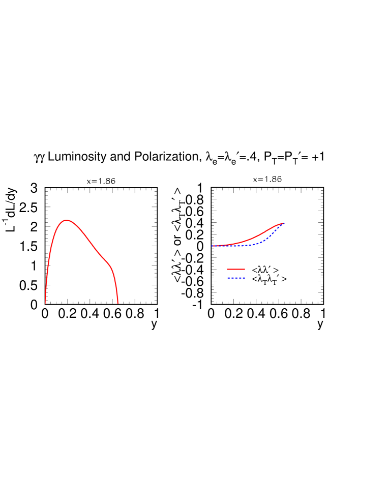
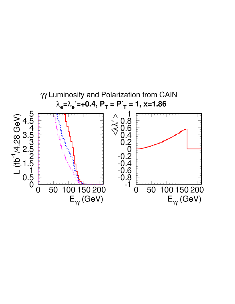
Figure 20: We plot the luminosities and corresponding $\langle\lambda\lambda^{\prime}\rangle$ and $\langle\lambda_{T}\lambda_{T}^{\prime}\rangle$ for operation at $\sqrt{s}=206~{}{\rm GeV}$ and $x=1.86$, assuming 100% transverse polarization for the laser photons and $\lambda_{e}=\lambda_{e}^{\prime}=0.4$. These plots are for the naive non-CAIN distributions.

Figure 21: We plot the luminosity, $L=d{\cal L}/dE_{\gamma\gamma}$, in units of $~{}{\rm fb}^{-1}/4.28~{}{\rm GeV}$ and corresponding $\langle\lambda\lambda^{\prime}\rangle$ predicted by CAIN for operation at $\sqrt{s}=206~{}{\rm GeV}$ and $x=1.86$, assuming 100% transverse polarization for the laser photons and $\lambda_{e}=\lambda_{e}^{\prime}=0.4$. The dashed (dotted) curve gives the component of the total luminosity that derives from the $J_{z}=0$ ($J_{z}=2$) two-photon configuration. The solid luminosity curve is the sum of these two components and $\langle\lambda\lambda^{\prime}\rangle=(L_{J_{z}=0}-L_{J_{z}=2})/(L_{J_{z}=0}+L_{J_{z}=2})$.

Using the naive analytic forms for back-scattered photon luminosities and polarizations, one finds that for 100% transverse polarization of the laser photon, the transverse polarization of the back-scattered photon is given by the electron-polarization-independent form

$$\lambda_{T}={2r^{2}\over(1-z)^{-1}+(1-z)-4r(1-r)}\,,$$ (14)

where $\lambda_{T}$ is the appropriate Stoke’s parameter and $r=zx^{-1}/(1-z)$ with $z=E_{\gamma}/E_{e^{-}}$. The maximum of $\lambda_{T}$,

$$\lambda_{T}^{\rm max}=2(1+x)/[1+(1+x)^{2}],$$ (15)

occurs at the kinematic limit, $z_{\rm max}=x/(1+x)$ (i.e. $r=1$). This can be compared to the analytic form for the longitudinal polarization:

$$\lambda={2\lambda_{e}rx[1+(1-z)(2r-1)^{2}]\over(1-z)^{-1}+(1-z)-4r(1-r)}\,.$$ (16)

At the kinematic limit, $z=z_{\rm max}=x/(1+x)$, the ratio of $\lambda$ to $\lambda_{T}$ is given by

$${\lambda\over\lambda_{T}}=\lambda_{e}x{2+x\over 1+x}\sim 1$$ (17)

for $\lambda_{e}=0.4$ and $x=1.86$. Substantial luminosity and values of $\lambda_{T}$ close to the maximum are achieved for moderately smaller $z$. From (14), operation at $x=1.86$ (corresponding to $\sqrt{s}=206~{}{\rm GeV}$ and laser wave length of $\lambda\sim 1~{}\mu$) would allow $\lambda_{T}^{\rm max}\sim\lambda^{\rm max}\sim 0.6$. Making these choices for both beams is very nearly optimal for the CP study for the following reasons. First, these choices will maximize ${d{\cal L}\over dE_{\gamma\gamma}}\langle\lambda_{T}\lambda_{T}^{\prime}\rangle$ at ${E_{\gamma\gamma}=120~{}{\rm GeV}}$. As seen from earlier equations, it is the square root of the former quantity that essentially determines the accuracy with which the CP determination can be made. Second, $\lambda_{e}=\lambda_{e}^{\prime}=0.4$ results in $\langle\lambda\lambda^{\prime}\rangle>0$. This is desirable for suppressing the background. (If there were no background, Eq. (13) implies that the optimal choice would be to employ $\lambda_{e}$ and $\lambda_{e}^{\prime}$ such that $\langle\lambda\lambda^{\prime}\rangle<0$. However, in practice the background is very substantial and it is very important to have $\langle\lambda\lambda^{\prime}\rangle>0$ to suppress it as much as possible.) In Fig. 21, we plot the naive luminosity distribution and associated values of $\langle\lambda\lambda^{\prime}\rangle$ and $\langle\lambda_{T}\lambda_{T}^{\prime}\rangle$ obtained for $\lambda_{e}=\lambda_{e}^{\prime}=0.4$ and 100% transverse polarization for the laser beams.

As discussed in [33], the asymmetry studies discussed below are not very sensitive to the polarization of the colliding $e$ beams. Thus, the studies could be performed in parasitic fashion during $e^{-}e^{+}$ operation if the $e^{+}$ polarization is small. (As emphasized earlier, substantial $e^{+}$ polarization would be needed for precision studies of other $h_{SM}$ properties.)

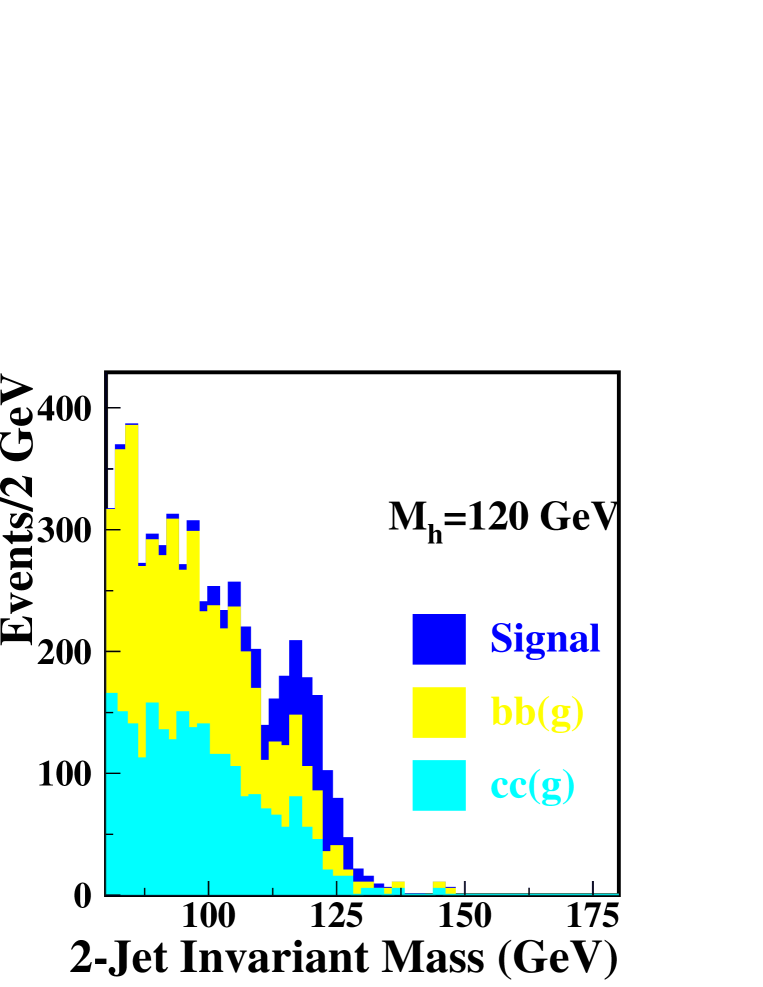
Figure 22: We plot the signal and $b\overline{b}$ and $c\overline{c}$ backgrounds for a SM Higgs boson with $m_{h_{SM}}=120~{}{\rm GeV}$ assuming $\gamma\gamma$ operation at $\sqrt{s}=206~{}{\rm GeV}$ and $x=1.86$, based on the luminosity and polarization distributions of Fig. 21 for the case of linearly polarized laser photons. The cross sections presented are those for $\delta=\pi/4$, i.e. in the absence of any contribution from the transverse polarization term in Eq. (12).

The luminosity distribution predicted by the CAIN Monte Carlo for transversely polarized laser photons and the corresponding result for $\langle\lambda\lambda^{\prime}\rangle$ are plotted in Fig. 21. We note that even though the luminosity spectrum is not peaked, it is very nearly the same at $E_{\gamma\gamma}=120~{}{\rm GeV}$ as in the circular polarization case. As expected from our earlier discussion of the naive luminosity distribution, at $E_{\gamma\gamma}=120~{}{\rm GeV}$ we find $\langle\lambda\lambda^{\prime}\rangle\sim\langle\lambda_{T}\lambda_{T}^{\prime}\rangle\sim 0.36$. Since CAIN includes multiple interactions and non-linear Compton processes, the luminosity is actually non-zero for $E_{\gamma\gamma}$ values above the naive kinematic limit of $\sim 132~{}{\rm GeV}$. Both $\langle\lambda\lambda^{\prime}\rangle$ and $\langle\lambda_{T}\lambda_{T}^{\prime}\rangle$ continue to increase as one enters this region. However, the luminosity becomes so small that we cannot make effective use of this region for this study. We employ these luminosity and polarization results in the vicinity of $E_{\gamma\gamma}=120~{}{\rm GeV}$ in a full Monte Carlo for Higgs production and decay as outlined earlier in the circular polarization case. All the same cuts and procedures are employed.

The resulting signal and background rates for $\delta=\pi/4$ are presented in Fig. 22. The width of the Higgs resonance peak is $5.0\pm 0.3~{}{\rm GeV}$ (using a Gaussian fit), only slightly larger than in the circularly polarized case. However, because of the shape of the luminosity distribution, the backgrounds rise more rapidly for $m_{b\overline{b}}$ values below $120~{}{\rm GeV}$ than in the case of circularly polarized laser beams. Thus, it is best to use a slightly higher cut on the $m_{b\overline{b}}$ values in order to obtain the best statistical significance for the signal. We find $\sim 360$ reconstructed two-jet signal events with $m_{b\overline{b}}\geq 114~{}{\rm GeV}$ in one year of operation, with roughly 440 background events in this same region. This corresponds to a precision of $\sqrt{S+B}/S\sim 0.079$ for the measurement of $\Gamma(h_{SM}\to\gamma\gamma)BR(h_{SM}\to b\overline{b})$. Not surprisingly, this is not as good as for the circularly polarized setup, but it is still indicative of a very strong Higgs signal. Turning to the CP determination, let us assume that we run 1/2 year in the parallel polarization configuration and 1/2 year in the perpendicular polarization configuration. Then, because we have only 60% linear polarization for the colliding photons for $E_{\gamma\gamma}\sim 120~{}{\rm GeV}$, $N_{\parallel}\sim 180[1+(0.6)^{2}]+273\sim 518$ and $N_{\perp}\sim 180[1-(0.6)^{2}]+273=388$. For these numbers, ${\cal A}=130/906\sim 0.14$. The error in ${\cal A}$ is $\delta{\cal A}=\sqrt{N_{\parallel}N_{\perp}/N^{3}}\sim 0.016$ ($N\equiv N_{\parallel}+N_{\perp}$), yielding ${\delta{\cal A}\over{\cal A}}={\delta{\cal CP}\over{\cal CP}}\sim 0.11$. This measurement would thus provide a fairly strong confirmation of the CP=+ nature of the $h_{SM}$ after one $10^{7}$ sec year devoted to this study.

8 Conclusions

In this paper, we have explored the various ways in which a $\gamma\gamma$ collider could contribute to our understanding of Higgs physics. We have confined our study to the $b\overline{b}$ final state. We have shown the following.

• For a SM-like Higgs boson, it will be possible to determine $\Gamma(\gamma\gamma\to h)BR(h\to b\overline{b})$ with excellent precision, e.g. $\sim 2.9\%$ accuracy for $m_{h}\sim 120~{}{\rm GeV}$. This accuracy will be achieved after just one $10^{7}$ sec year of operation, using the frequency tripler technology and a peaked $E_{\gamma\gamma}$ spectrum is the most optimal.

  By using the excellent $\sim 1\%-2\%$ measurement of $BR(h\to b\overline{b})$, one can extract a $\sim 2.9\%$ measurement for $\Gamma(h\to\gamma\gamma)$. As discussed in the introduction, deviations of this width from its SM expectations could be very revealing. In particular, at this level of accuracy, deviations that might be present as the result of the SM-like Higgs boson being part of a larger Higgs sector, such as that of the MSSM, would typically be visible if some of the other Higgs bosons were not too much heavier than $500~{}{\rm GeV}$ or so. In the MSSM context, the precise magnitude of the deviations might thus allow extraction of the crucial mass scale $m_{A^{0}}$. If $m_{A^{0}}$ is known with sufficient accuracy, one would know more or less exactly what $\sqrt{s}$ to employ so that detection of $\gamma\gamma\to A^{0},H^{0}$ at the $\gamma\gamma$ collider would be straightforward and would become a high priority.

• Even if there is no predetermination of $m_{A^{0}}$, detection of $\gamma\gamma\to H^{0},A^{0}$ is still likely to be possible for a large fraction of the problematical ‘wedge’ of moderate-$\tan\beta$ parameter space, described earlier, for which the $H^{0},A^{0}$ will not be observable either at the LHC or at a LC. For instance, for a LC of $\sqrt{s}=630~{}{\rm GeV}$, the wedge begins at $m_{A^{0}}\mathrel{\raise 1.29167pt\hbox{$>$\kern-7.5pt\lower 4.30554pt\hbox{$\sim$}}}300~{}{\rm GeV}$ (the approximate upper reach of the $e^{+}e^{-}\to H^{0}A^{0}$ pair production process) whereas the $\gamma\gamma$ collider can potentially allow detection of the $H^{0},A^{0}$ up to the $E_{\gamma\gamma}$ spectrum limit of about 500 GeV. Indeed, using just $b\overline{b}$ final states, our results show that $H^{0},A^{0}$ detection will be possible in somewhat more than 65% of the wedge after two ($10^{7}$ sec) years of operation using a broad spectrum and one year of operation using a peaked spectrum. By also considering $H^{0}\to h^{0}h^{0}$, $A^{0}\to Zh^{0}$ and $H^{0},A^{0}\to t\overline{t}$ final states, we estimate that somewhat more than 85% of the wedge parameter region with $m_{A^{0}}\mathrel{\raise 1.29167pt\hbox{$<$\kern-7.5pt\lower 4.30554pt\hbox{$\sim$}}}500~{}{\rm GeV}$ would provide a detectable signal after a total of two to three years of operation.

  Thus, by combining $\sqrt{s}=630~{}{\rm GeV}$ $\gamma\gamma$ collider operation with LC studies of $e^{+}e^{-}$ collisions and LHC searches for the MSSM Higgs bosons, we would have an excellent chance of finding all the neutral Higgs bosons of the MSSM Higgs sector (if they have mass $\mathrel{\raise 1.29167pt\hbox{$<$\kern-7.5pt\lower 4.30554pt\hbox{$\sim$}}}500~{}{\rm GeV}$), whereas without the $\gamma\gamma$ collider one would detect only the $h^{0}$ (at both the LC and LHC) in the problematical parameter space wedge. In short, if we detect supersymmetric particles at the LHC and LC consistent with the MSSM structure and find only the $h^{0}$ at the LC and LHC, $\gamma\gamma$ operation focusing on Higgs discovery will be a high priority.

• The one caveat to this very optimistic set of conclusions regarding the $H^{0},A^{0}$ is that if SUSY particles are light (masses $\mathrel{\raise 1.29167pt\hbox{$<$\kern-7.5pt\lower 4.30554pt\hbox{$\sim$}}}m_{A^{0}}/2$), they will alter the predictions for the $H^{0},A^{0}\to\gamma\gamma$ couplings and diminish the $H^{0},A^{0}\to b\overline{b}$ branching ratios. If these effects are very strong, as possible at lower $\tan\beta$, detection of the $H^{0},A^{0}$ in the $b\overline{b}$ channel could become significantly more difficult, both in $\gamma\gamma$ collisions and at the LHC — SUSY decay channels would need to be employed. However, at the larger $\tan\beta$ values in the wedge region under consideration, the $b\overline{b}$ coupling is strongly enhanced and it is unlikely that these effects would be sufficiently large to significantly alter our conclusions.

• It is important to note that the $\gamma\gamma\to H^{0},A^{0}\to b\overline{b}$ rate has a minimum at $\tan\beta\sim 15$ ($\tan\beta\sim 20$) for $m_{A^{0}}\mathrel{\raise 1.29167pt\hbox{$<$\kern-7.5pt\lower 4.30554pt\hbox{$\sim$}}}300~{}{\rm GeV}$ ($m_{A^{0}}\geq 350~{}{\rm GeV}$), i.e. $\tan\beta$ values that are just large enough to be above the wedge region at higher $m_{A^{0}}$. Thus, the $\gamma\gamma\to H^{0},A^{0}\to b\overline{b}$ rate increases for still higher $\tan\beta$ (roughly linearly for $\tan\beta$ in the $30-50$ range). Consequently, if the $H^{0},A^{0}$ are discovered at the LHC because $\tan\beta$ is large, and yet other physics considerations force $\gamma\gamma$ operation at maximal $\sqrt{s}$ (rather than at the $\sqrt{s}$ such that $E_{\rm peak}\sim m_{A^{0}}$) there is a good possibility that the $\gamma\gamma\to H^{0},A^{0}\to b\overline{b}$ signal will be quite substantial (if one chooses the appropriate, type-I or type-II, spectrum for the $m_{A^{0}}$ value found at the LHC). This would then provide an opportunity for a relatively precise measurement of the very interesting $\gamma\gamma\to H^{0},A^{0}$ couplings that will not be accessible by any other means. This in turn could lead to significant information about other SUSY parameters. In particular, as illustrated in the main part of the paper, $\tan\beta$ can be determined with reasonable accuracy from the $\gamma\gamma\to H^{0},A^{0}\to b\overline{b}$ rate if the masses and properties of the SUSY particles are known from LHC and/or LC data. Most notably, the larger $\tan\beta$ is, the more accurate will be this determination. In contrast, most other techniques for determining $\tan\beta$ (e.g. from neutralino, chargino, gluino, etc. cross sections and branching ratios) become increasingly insensitive to $\tan\beta$ as $\tan\beta$ increases.

• After three ($10^{7}$ sec) years of operation (2 with type-I spectrum and 1 with type-II spectrum), it will be possible to detect the $A^{0}$ of a general two-Higgs-double model (in particular, one with parameters such that all other Higgs bosons are heavy, including the SM-like neutral Higgs) over a substantial portion of the parameter space in which it cannot be detected in any other LC or LHC modes.

• Determination of the CP nature of any Higgs boson that can be observed will be possible in $\gamma\gamma$ collisions by employing transversely (linearly) polarized laser beam photons. In particular, we studied the case of a light SM-like Higgs boson with $m_{h}=120~{}{\rm GeV}$, and showed that the error in determination of its ${\cal CP}=+1$ would be $\delta{\cal CP}/{\cal CP}\sim 0.11$.

For these various purposes, there is no question that maximizing the luminosity will be very important. In the case of the NLC design we consider, the results stated above would require 1 $10^{7}$ sec year of operation at low $\sqrt{s}$ for the light Higgs precision study, 1 year of operation at low $\sqrt{s}$ in the linearly polarized mode for the ${\cal CP}$ study, and 3 years of operation for the $H^{0},A^{0}$ search (one in the peaked spectrum mode and two in the broad spectrum mode if one is constrained to run at the maximal $\sqrt{s}=630~{}{\rm GeV}$ assumed in our study). The extra factor of 2 in luminosity that might be achievable at TESLA would prove an advantage. Further optimization of the NLC design might also be possible and is strongly encouraged. For instance, going to a round beam configuration keeping the CP-IP separation at 1 mm might yield as much as a factor of two increase in luminosity.

We should note that our studies have only included hadronic backgrounds due to direct (QED) processes and have not yet incorporated backgrounds resulting from the hadronic structure of the photon. The photon can “resolve” into quarks or gluons plus spectator jets. Hadronic production could then occur through $\gamma\gamma^{*}$ (1-resolved) or $\gamma^{*}\gamma^{*}$ (2-resolved) processes. Resolved photon backgrounds have two contributions to the background to Higgs production. The first is that in which a quark or gluon ‘constituent’ of one of the back-scattered photons is responsible for initiating a two-body scattering process that creates a pair of high-$p_{T}$ $b$ or $c$ jets. (As discussed, for example, in Ref. [34] good $b$-tagging efficiency and purity, as employed here, is required in order to eliminate other resolved photon two-jet backgrounds, such as $gb$ or $gc$ final states.) However, it is generally the case that such contributions to the background are numerically unimportant unless the Higgs mass is far below the maximum $E_{\gamma\gamma}$. This was first concluded in Ref. [34] and more recently confirmed in Ref. [21]. In the $m_{h}=120~{}{\rm GeV}$ cases we study, the Higgs mass is quite close to the maximum $\gamma\gamma$ energy, and in the $H^{0},A^{0}$ studies the Higgs mass is at least 50% of the maximum $\gamma\gamma$ energy. For such choices, this kind of resolved photon background is not important. In addition, any residual resolved photon background of this type could be further reduced by vetoing events in which there is an extra “remnant” jet in the forward and/or backward region — such jets would tend to have transverse and longitudinal momentum of order ${\textstyle{1\over 3}}m_{h}$ to ${\textstyle{1\over 2}}m_{h}$ for the configurations we employ and would, therefore, be readily visible in the detector.

The second type of background from resolved photon processes arises when a resolved photon scattering process underlies the primary Higgs production reaction. These events arise when back-scattered photons other than those involved in the Higgs production reaction also interact. This can happen either using back scattered photons arising in the same bunch crossing or photons from two different bunch crossings within the same detector readout interval. Cross sections (before cuts) for producing relatively soft jets deriving from these resolved photon processes are several orders of magnitude larger than the corresponding direct $\gamma\gamma\to X$ cross section. Thus, such additional scatterings primarily yield additional low-$p_{T}$ jets that would underlie the $b\overline{b}$ jets arising from Higgs production. They would thus make it less efficient to isolate the true 2-$b$-jet signal using cuts that require exactly two reconstructed jets which are rather precisely back-to-back. Mass resolution could also deteriorate, as might the efficiency for $b$-tagging. The level of this background is determined by the number of back-scattered photons created in each bunch crossing as well as the number of bunch crossings over which the detector integrates. At TESLA, the bunch spacing is 337 ns and it might be possible to design the detector so that there would be only one crossing per detector readout. In this case, only the underlying $\gamma\gamma$ interactions from this single crossing would need to be considered. For the NLC parameters considered here, the bunch spacing is only 2.8 ns (as desirable for $\gamma\gamma$ operation in order to maximize the bunch charge for the same total current). In general, the detector will integrate over a number of bunch crossings and it will therefore be desirable to minimize this number. This may turn out to be an important factor in determining the NLC detector design. On the other hand, although it may only be necessary to integrate over one bunch crossing at TESLA, the bunch charge will be roughly 30% higher and there will be more back-scattered photons (that can give rise to underlying $\gamma\gamma$ interactions) per crossing than for the NLC design. Thus, a detailed examination of this background is required in both the TESLA and NLC cases. In particular, the performance of the $b$-tagging and energy flow algorithms will be critical and will depend upon the occupancies in the vertex detector and calorimeter, respectively. Overall, our ability to reconstruct the (two-jet) component of the Higgs resonance in the presence of underlying soft jet structure from resolved photon interactions is critically dependent upon detector design features. Absent the required studies in the context of a detailed detector design, we cannot currently determine whether the resulting resolved photon backgrounds will be a problem at either machine or which machine will yield the smallest resolved photon background.

We should note that our results have assumed 80% polarization for both the $e$ beams used to back-scatter the laser photons. Only the ${\cal CP}$ studies would remain little altered if one of the beams does not have substantial polarization. Because of substantially increased background levels, comparable results for the other studies/searches would require significantly more integrated luminosity if only one beam has large polarization. As a result, if one is to be able to perform these $\gamma\gamma$ studies parasitically during normal $e^{+}e^{-}$ operation of the LC, substantial $e^{+}$ polarization will be very important. Another issue related to simultaneously studying $e^{+}e^{-}$ collisions and $\gamma\gamma$ interactions is the bunch spacing. If the design $1.4$ ns bunch spacing for $e^{+}e^{-}$ is employed, then our luminosities will be decreased by about 40%.

Acknowledgments

We would like to thank M. Battaglia, T. Hill, M. Spira, V. Telnov, M. Velasco and P. Zerwas for useful discussions.

9 Appendix A

In this Appendix, we give the machine and beam parameters that we have assumed in computing $\gamma\gamma$ luminosities (using the CAIN Monte Carlo) for the various running options considered in this paper. These parameters are presented in Table 5.

Table 5: Parameters for the various beam energy and polarization options considered in this paper.

Energy (GeV)	80	103	267.5	315
$\beta_{x}/\beta_{y}$ (mm)	1.4/0.08	1.5/0.08	4/0.065	4/0.08
$\epsilon_{x}/\epsilon_{y}~{}(\times 10^{-8})$	360/7.1	360/7.1	360/7.1	360/7.1
$\sigma_{x}/\sigma_{y}~{}({\rm nm})$	179/6.0	0 164/5.3	166/3.0	153/3.0
$\sigma_{z}$ (microns)	156	156	156	156
$N~{}(\times 10^{10})$	1.5	1.5	1.5	1.5
$e^{-}~{}{\rm Polarization}~{}(\%)$	80	80	80	80
repetition rate (Hz)	120$\times$95	120$\times$95	120$\times$95	120$\times$95
Laser $\lambda$ (microns)	0.351	1.054	1.054	1.054
CP-IP distance (mm)	1	1	1	1

We note that our designs have emphasized fairly flat beams which would be most appropriate if the $\gamma\gamma$ collider interaction region is running parasitically at the same time as the main interaction region is exploring $e^{-}e^{-}$ collisions.

10 Appendix B: Higher-order corrections

Papers that have considered higher order QCD corrections to Higgs production and the background cross sections, and that have examined implications for Higgs detection include [35, 36, 22, 23, 9, 10, 37]. Some of the corrections found in these papers are large under certain circumstance. The purpose of this appendix is to explain why these corrections are relatively small for the cuts and the colliding photon luminosities and polarizations (predicted by CAIN) employed and to demonstrate that it is much more important to have as accurate a simulation as possible in a realistic experimental approach.

Let us discuss the background cross sections first. The tree-level $J_{z}=0$ and $J_{z}=\pm 2$ cross sections are given in Eqs. (3) and (4). The $m_{q}^{2}/s$ suppression of the $J_{z}=0$ background implies that radiative corrections to this component of the cross section can be large. The exact magnitude of these corrections depends critically upon the laser beam configuration (in particular, circular or linear) and the precise cuts employed. The radiative corrections are dramatically reduced by employing cuts that isolate two-jet final states. In the case of circularly polarized laser beams, if two-jet final states are isolated by employing $y_{\rm cut}=0.02$ (the first of the two-jet cuts we use) the $J_{z}=0$ background can still be increased relative to the tree-level expectation by up to a factor of 10 [16]. This factor will be reduced by the additional back-to-back cut that we employ (which also discriminates against the radiation of an additional gluon at the partonic level), but still might be large. In contrast, radiative corrections to the $J_{z}=\pm 2$ background cross sections are relatively small ($\mathrel{\raise 1.29167pt\hbox{$<$\kern-7.5pt\lower 4.30554pt\hbox{$\sim$}}}10\%$ typically [16]). For linearly polarized laser beams, the higher-order corrections to the two-jet final states are quite modest in size [37]. Thus, the most important question is whether or not we need to worry about the large corrections to the $J_{z}=0$ background in the case of circularly polarized laser beams.

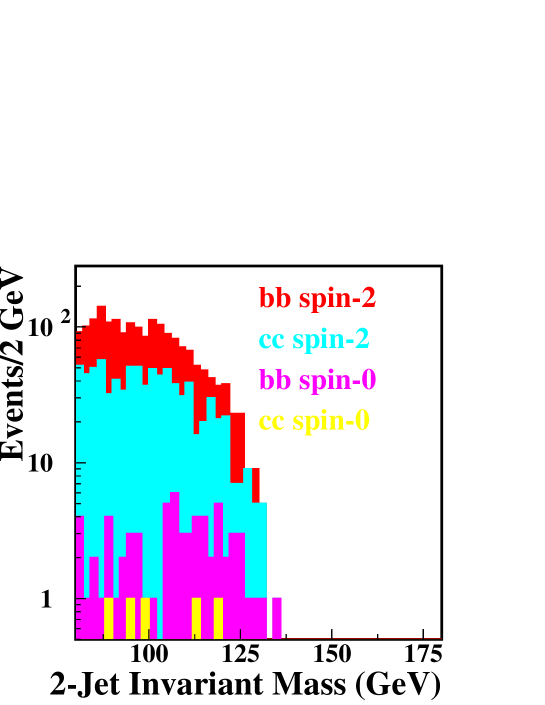
Figure 23: For $\sqrt{s}=160~{}{\rm GeV}$ and frequency tripler operation, we plot, as a function of 2-jet mass (in GeV), the $J_{z}=0$ and $J_{z}=2$ backgrounds (events per $10^{7}$ sec year per bin) for $c\overline{c}(g)$ and $b\overline{b}(g)$ production as obtained from PYTHIA (modified to incorporate correct tree-level $J_{z}=0$ and $J_{z}=2$ cross sections) with processing via JETSET and ROOT after all cuts, most especially including cuts imposed to isolate only the 2 jet final state. Colliding photon luminosities and polarizations employed are those predicted by the CAIN Monte Carlo assuming 100% circular polarization ($P_{c}=P_{c}^{\prime}=-1$) for the laser beams and 80% polarization ($\lambda_{e}=\lambda_{e}^{\prime}=0.4$) for the electron beams.

In Fig. 23, we plot the tree-level predictions for the $J_{z}=0$ and $J_{z}=\pm 2$ $c\overline{c}(g)$ and $b\overline{b}(g)$ backgrounds obtained by running PYTHIA/JETSET and processing using ROOT to impose the 2-jet final state cuts delineated in the main body of the paper. The sum of the $J_{z}=0$ and $J_{z}=\pm 2$ backgrounds plotted in this figure gives the net backgrounds displayed in Fig. 3 for the SM Higgs boson with mass of 120 GeV. These background levels include the expected luminosity from CAIN in the $J_{z}=0$ and $J_{z}=\pm 2$ initial two-photon configurations for 80% electron beam polarization. What is immediately apparent is that the background is overwhelmingly dominated by the $J_{z}=\pm 2$ backgrounds. From Fig. 23 we see that even if the QCD corrections to the $J_{z}=0$ backgrounds were as large as a factor of 10, this would affect the total background at a level no greater than 20%. This conclusion differs from that of previous works largely due to to the fact that the value of $\langle\lambda\lambda^{\prime}\rangle$ obtained in CAIN and assuming the fairly realistic 80% polarizations ($\lambda_{e}=\lambda_{e}^{\prime}=0.4$) is not sufficiently close to unity to more than partially suppress the $J_{z}=\pm 2$ background.

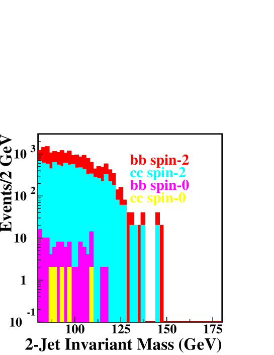
Figure 24: For $\sqrt{s}=206~{}{\rm GeV}$ and without frequency tripler operation, we plot, as a function of 2-jet mass (in GeV), the $J_{z}=0$ and $J_{z}=2$ backgrounds (events per $10^{7}$ sec year per bin) for $c\overline{c}(g)$ and $b\overline{b}(g)$ production as obtained from PYTHIA (modified to incorporate correct tree-level $J_{z}=0$ and $J_{z}=2$ cross sections) with processing via JETSET and ROOT after all cuts, most especially including cuts imposed to isolate only the 2 jet final state. Colliding photon luminosities and polarizations employed are those predicted by the CAIN Monte Carlo assuming 100% linear polarization for the laser beams and 80% polarization ($\lambda_{e}=\lambda_{e}^{\prime}=0.4$) for the electron beams.

In Fig. 24, we plot the tree-level predictions for the $J_{z}=0$ and $J_{z}=\pm 2$ $c\overline{c}(g)$ and $b\overline{b}(g)$ backgrounds in the case of linearly polarized laser beams as employed in constructing Fig. 22. As above, these were obtained by running PYTHIA/JETSET and processing using ROOT to impose the 2-jet final state cuts delineated in the main body of the paper. The sum of the $J_{z}=0$ and $J_{z}=\pm 2$ backgrounds plotted in this figure gives the net backgrounds displayed in Fig. 22 for the SM Higgs boson with mass of 120 GeV. These background levels include the expected luminosity from CAIN in the $J_{z}=0$ and $J_{z}=\pm 2$ initial two-photon configurations for 80% electron beam polarization. As for the case of circularly polarized laser beams, the background is overwhelmingly dominated by the $J_{z}=\pm 2$ backgrounds. QCD NLO and resummation corrections to the $J_{z}=0$ two-jet cross section in the case of linearly polarized laser beams are expected to be much more modest in size than in the case of circularly polarized beams [37]. But, even if these corrections were to increase the $J_{z}=0$ backgrounds by as much as a factor of 10, the background level would be only of order $3\%$ larger than that we have employed.

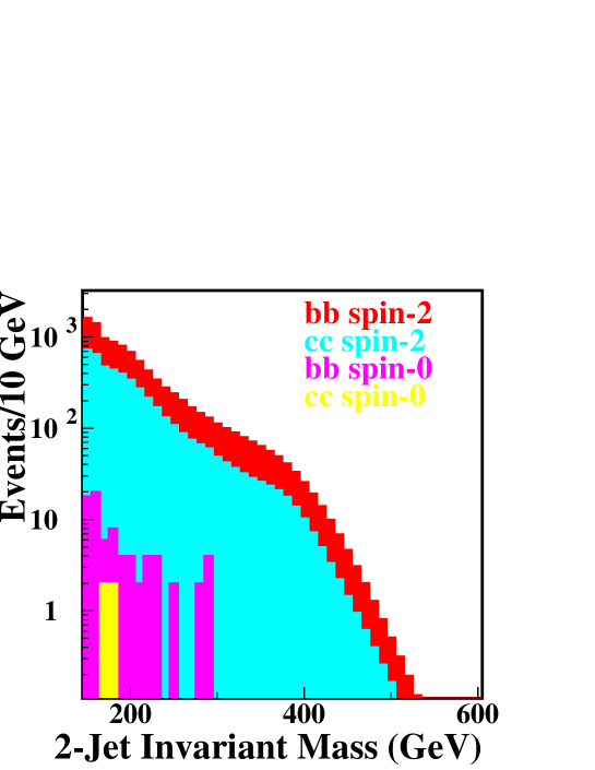
Figure 25: For $\sqrt{s}=630~{}{\rm GeV}$ and type-I (broad spectrum) polarization configuration operation, we plot, as a function of 2-jet mass (in GeV), the $J_{z}=0$ and $J_{z}=2$ backgrounds (events per $10^{7}$ sec year per bin) for $c\overline{c}(g)$ and $b\overline{b}(g)$ production as obtained from PYTHIA/JETSET/ROOT after all cuts. Colliding photon luminosities and polarizations employed are those predicted by the CAIN Monte Carlo assuming 100% circular polarization ($P_{c}=P_{c}^{\prime}=+1$) for the laser beams and 80% polarization ($\lambda_{e}=\lambda_{e}^{\prime}=0.4$) for the electron beams.

Figs. 25 and 26 give the $J_{z}=0$ and $J_{z}=\pm 2$ backgrounds incorporated in the $\sqrt{s}=630~{}{\rm GeV}$ Figs. 11 and 12 in the cases of type-I (broad spectrum) and type-II (peaked spectrum) operation, respectively; these are the results after all cuts, including the 2-jet cuts. We see that even a factor of 10 QCD correction to the $J_{z}=0$ portion of the background would result in at most a 10% correction to the total background. Let us compare this situation to [9] (see [10] for details). There, the background is dominated by the $J_{z}=0$ contribution and QCD corrections are essential for obtaining an appropriate background estimate. Although our signal cross section in the ‘without SUSY’ case is very close in value to that is plotted in Fig. 2 of [9] (if we convert our $I_{\sigma}$ to the cross section definition implicit in their figure), their background (obtained, we believe, assuming 100% electron polarization, $\lambda_{e}=\lambda_{e}^{\prime}=0.5$ — see comment below Eq. (3.61) in association with Fig. 3.12 of [10]) is much smaller than their signal. This is in sharp contrast to the background level we obtain in the CAIN simulation with 80% polarization ($\lambda_{e}=\lambda_{e}^{\prime}=0.4$), which background is quite comparable to our typical signal.

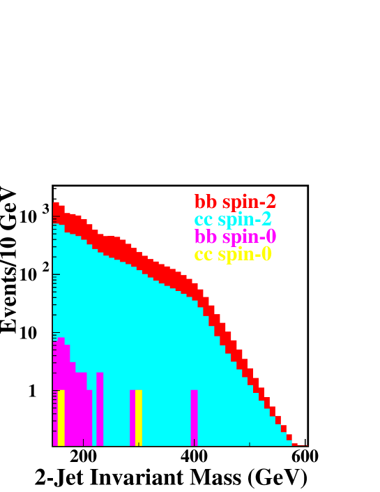
Figure 26: As in Fig. 25 except for type-II (peaked spectrum) polarization configuration ($P_{c}=P_{c}^{\prime}=-1$, $\lambda_{e}=\lambda_{e}^{\prime}=0.4$).

Another theoretical issue concerns the suppression factors associated with imposing 2-jet cuts on the signal. Our approach has been to generate the signal at tree-level but in the context of PANDORA/PYTHIA/JETSET which allows for the generation of extra jets via final state radiation. The imposition of 2-jet cuts will then give rise to a suppression factor as computed in the context of PYTHIA/JETSET, which factor is expected to be quite similar to that obtained from the analytic approaches but will also take into account experimental issues related to jet definition, detector resolutions and so forth. In this regard, it is useful to compare to Ref. [21], which follows an approach very similar to ours. Their Fig. 1 shows that before cuts about 75% of the Higgs events have more than 2 jets (using $y_{\rm cut}=0.02$). For the same Higgs mass, we obtain almost exactly the same result. Further, we find that this same percentage applies also for Higgs masses in the $300-500~{}{\rm GeV}$ range. A corresponding result is not given in [21] after imposing their cuts. In our case, after cuts, especially the back-to-back and $|\cos\theta^{*}|<0.5$ cuts, we find that roughly 90% (95%) of the events are 2-jet for Higgs masses of $120~{}{\rm GeV}$ ($400~{}{\rm GeV}$).

The final theoretical issue that requires discussion is the possible importance of interference between signal and background. Here, we refer to several discussions in [10]. First, as shown in their Eq. (3.22), we note that the interference cross section only involves the $J_{z}=0$ part of the background. Since the Higgs bosons being considered are essentially produced on-shell, and since after cuts the $J_{z}=0$ backgrounds are reduced to a level much smaller than the signal cross section, such interference will be small. For example, [10] (see below Eq. (3.64)) finds that the interference cross section is typically of order 1/100 to 1/1000 of the signal cross section after imposing cuts similar those we consider.

Grant Support

This work was supported in part by the U.S. Department of Energy contract No. DE-FG03-91ER40674 and under the auspices of the U.S. Department of Energy by the University of California, Lawrence Livermore National Laboratory under Contract No.W-7405-Eng.48.

References

- [1] J. F. Gunion and H. E. Haber, Phys. Rev. D 48, 5109 (1993).
- [2] D. L. Borden, D. A. Bauer and D. O. Caldwell, Phys. Rev. D 48, 4018 (1993).
- [3] T. Abe et al. [American Linear Collider Working Group Collaboration], hep-ex/0106058.
- [4] K. Abe et al., hep-ph/0109166.
- [5] T. Abe et al. [American Linear Collider Working Group Collaboration], SLAC-R-570 Resource book for Snowmass 2001, 30 Jun - 21 Jul 2001, Snowmass, Colorado.
- [6] J. A. Aguilar-Saavedra et al. [ECFA/DESY LC Physics Working Group Collaboration], “TESLA Technical Design Report Part III: Physics at an e+e- Linear Collider,” hep-ph/0106315.
- [7] J.F. Gunion, H. Haber, H. Logan, and S. Mrenna, work in progress.
- [8] B. Grzadkowski, J. F. Gunion and J. Kalinowski, Phys. Lett. B 480, 287 (2000) [hep-ph/0001093].
- [9] M. M. Muhlleitner, M. Kramer, M. Spira and P. M. Zerwas, Phys. Lett. B 508, 311 (2001) [arXiv:hep-ph/0101083].
- [10] M. M. Muhlleitner, arXiv:hep-ph/0008127.
- [11] P. Chankowski, T. Farris, B. Grzadkowski, J. F. Gunion, J. Kalinowski and M. Krawczyk, Phys. Lett. B 496, 195 (2000) [hep-ph/0009271].
- [12] J. F. Gunion, J. G. Kelly and J. Ohnemus, Phys. Rev. D 51, 2101 (1995) [hep-ph/9409357].
- [13] J. F. Gunion and J. Kelly, Phys. Rev. D 56, 1730 (1997) [hep-ph/9610495].
- [14] J. F. Gunion and J. Kelly, hep-ph/9610421.
- [15] J. L. Feng and T. Moroi, Phys. Rev. D 56, 5962 (1997) [hep-ph/9612333].
- [16] S. Söldner-Rembold, private communication.
- [17] I. F. Ginzburg, G. L. Kotkin, V. G. Serbo and V. I. Telnov, Nucl. Instrum. Meth. 205, 47 (1983).
- [18] I. F. Ginzburg, G. L. Kotkin, S. L. Panfil, V. G. Serbo and V. I. Telnov, Nucl. Instrum. Meth. A 219, 5 (1984).
- [19] Research aimed at improving polarization continues and could prove vital for the option. A recent discussion of possible technologies appears in Ref. [6].
- [20] P. Chen, G. Horton-Smith, T Ohgaki, A. W. Weidemann and K. Yokoya,, Nucl. Instrum. Meth. A355, 107 (1995). See http://www-acc-theory.kek.jp/members/cain/cain21b.manual/main.html.
- [21] G. Jikia and S. Soldner-Rembold, Nucl. Phys. Proc. Suppl. 82, 373 (2000) [arXiv:hep-ph/9910366].
- [22] M. Melles, W. J. Stirling and V. A. Khoze, Phys. Rev. D 61, 054015 (2000) [arXiv:hep-ph/9907238].
- [23] M. Melles and W. J. Stirling, Nucl. Phys. B 564, 325 (2000) [arXiv:hep-ph/9903507].
- [24] T. Sjostrand, hep-ph/9508391. T. Sjostrand, P. Eden, C. Friberg, L. Lonnblad, G. Miu, S. Mrenna and E. Norrbin, hep-ph/0010017. See the PYTHIA and JETSET web pages, http://www.thep.lu.se/ torbjorn/Pythia.html.
- [25] R. Brun and F. Rademakers, Nucl. Instrum. Meth. A 389, 81 (1997).
-
[26]
The PANDORA web
page is
http://www-sldnt.slac.stanford.edu/nld/new/Docs/Generators/PANDORA.htm. - [27] The results of Fig. 4 were provided by F. Gianotti and E. Richter-Was on behalf of the ATLAS collaboration. They are the preliminary results available as of September, 2001.
- [28] A. Djouadi, J. Kalinowski and M. Spira, Comput. Phys. Commun. 108, 56 (1998) [arXiv:hep-ph/9704448]. Programs are available at http://www.desy.de/ spira/proglist.html.
- [29] M. Carena, H. E. Haber, H. E. Logan and S. Mrenna, Phys. Rev. D 65, 055005 (2002) [Erratum-ibid. D 65, 099902 (2002)] [arXiv:hep-ph/0106116].
- [30] K. m. Cheung, C. H. Chou and O. C. Kong, Phys. Rev. D 64, 111301 (2001) [arXiv:hep-ph/0103183].
- [31] B. Grzadkowski and J. F. Gunion, Phys. Lett. B 294, 361 (1992) [hep-ph/9206262].
- [32] M. Kramer, J. Kuhn, M. L. Stong and P. M. Zerwas, Z. Phys. C 64, 21 (1994) [hep-ph/9404280].
- [33] J. F. Gunion and J. G. Kelly, Phys. Lett. B 333, 110 (1994) [hep-ph/9404343].
- [34] M. Baillargeon, G. Belanger and F. Boudjema, Phys. Rev. D 51, 4712 (1995) [arXiv:hep-ph/9409263].
- [35] D. L. Borden, V. A. Khoze, W. J. Stirling and J. Ohnemus, Phys. Rev. D 50, 4499 (1994) [arXiv:hep-ph/9405401].
- [36] G. Jikia and A. Tkabladze, Phys. Rev. D 54, 2030 (1996) [arXiv:hep-ph/9601384].
- [37] G. Jikia and A. Tkabladze, Phys. Rev. D 63, 074502 (2001) [arXiv:hep-ph/0004068].