DFF 376/09/2001 Statistical hadronisation model and transverse momentum spectra of hadrons in high energy collisions

Abstract

A detailed analysis of transverse momentum spectra of several identified hadrons in high energy collisions within the canonical framework of the statistical model of hadronisation is performed. The study of particle momentum spectra requires an extension of the statistical model formalism used to handle particle multiplicities, which is described in detail starting from a microcanonical treatment of single hadronising clusters. Also, a new treatment of extra strangeness suppression is presented which is based on the enforcement of fixed numbers of ${\rm s}\bar{\rm s}\;$pairs in the primary hadrons. The considered centre-of-mass energies range from $\simeq$ 10 to 30 GeV in hadronic collisions ($\pi$p, pp and Kp) and from $\simeq$ 15 to 35 GeV in e⁺e^-collisions. The effect of the decay chain following hadron generation is accurately and exhaustively taken into account by a newly proposed numerical method. The exact ${\bf p}_{T}$ conservation at low energy and the increasing hard parton emission at high energy bound the validity of the presently taken approach within a limited centre-of-mass energy range. However, within this region, a clear consistency is found between the temperature parameter extracted from the present analysis and that obtained from fits to average hadron multiplicities in the same collision systems. This finding indicates that in the hadronisation process the production of different particle species and their momentum spectra are two closely related phenomena governed by one parameter.

1 Introduction

The idea of a statistical approach to hadron production in high energy collisions dates back to ’50s fermi and ’60s hage and it has been recently revived by the observation that hadron multiplicities in e⁺e^-and pp collisions agree very well with a thermodynamical-like ansatz beca1 ; beca2 ; beca3 . This finding has also been confirmed in hadronic collisions and it has been interpreted in terms of a pure statistical filling of multi-hadronic phase space of assumed pre-hadronic clusters (or fireballs) formed in high-energy collisions, at a critical value of energy density beca3 ; heinz ; stock . In this framework, temperature and other thermodynamical quantities have a purely statistical meaning and do not involve the existence of a hadronic thermalisation process through multiple collisions on an event-by-event basis. Stated otherwise, statistical equilibrium is an intrinsic feature of the hadronisation process and hadrons are directly created in such a state beca3 ; heinz ; stock , as it was envisaged by Hagedorn hage2 .

So far, this proposed statistical cluster hadronisation model has been mainly tested against measured abundances of different hadron species for a twofold reason. Firstly, unlike momentum spectra, they are quantities which are not affected by hard (perturbative) QCD dynamical effects but are only determined by the hadronisation process; indeed, in the framework of a multi-cluster model, they are Lorentz invariant quantities which are independent of cluster’s overall momentum. Secondly, they are fairly easy to calculate and provide a very sensitive test of the model yielding an accurate determination of the temperature. However, in order to establish the validity of the model, it is necessary to test further observables and to assess their consistency with the results obtained for multiplicities. One of the best suited observables in this regard is the transverse momentum of identified hadrons (where transverse is meant to be with respect to beam line in high energy hadronic collision, and thrust or event axis in high energy e⁺e^-collisions) because, amongst all projections of particle momentum, this is supposed to be the most sensitive to hadronisation or, conversely, the least sensitive to perturbative QCD dynamics.

Actually, it has been known for a long time that transverse momentum spectra follow a Boltzmann distribution in hadronic collisions and this very observation was pointed out by Hagedorn as a major indication in favour of statistical hadron production hage3 . It must be emphasized that the prediction of a thermal-like shape in principle only applies to particles directly emitted from the hadronising source, whereas measured spectra also include particles produced by decays of heavier hadrons. Yet, due to involved calculations into play, most analyses do not take into account the distortion of primordial hadronisation spectrum induced by hadronic decays and try to fit the data straight through it. This problem has been discussed in literature hage4 and an analytical calculation has been developed to take into account the effect of two and three body decays sollfran ; sollfran2 , which has then been used both for pp sollfran2 and heavy ion collision sollfran ; sollfran2 ; wiedheinz ; peitzmann including most abundant resonances. In this paper we introduce a new method allowing to rigorously and exhaustively determine the contribution of all particle decays. Thence, by taking advantage of this technique, we have performed an analysis of many measured transverse momentum spectra of identified hadrons in a wide range of centre-of-mass energies for several kind of collisions.

The paper is organised as follows: in Sect. 2 the statistical hadronisation model is described in detail starting from a basic microcanonical treatment of clusters. In Sect. 3 the analytical formulae for transverse momentum spectra of hadrons within the statistical hadronisation model are derived whilst in Sect. 4 they are worked out for the primary and secondary component separately and the numerical method used to calculate them is described. In Sect. 5 and 6 the data analysis is presented and discussed. Conclusions are drawn in Sect. 7.

2 Statistical hadronisation model

The statistical hadronisation model assumes that in high energy collisions, as a consequence of strong interaction dynamics, a set of colour singlet clusters (or fireballs) endowed with mass, volume, internal quantum numbers and momentum, whose distribution is governed by the dynamical stage of the process, is formed. These clusters are supposed to give rise to hadrons according to a pure statistical law in the multi-hadronic phase space defined by their four-momentum, volume and quantum numbers. This approach differs from another popular cluster hadronisation model webber mainly because clusters are provided with a volume, so that hadron production is governed by proper phase space rather than relativistic momentum space. In this framework, the use of statistical mechanics and thermodynamical quantities, such as temperature, which needs spacial dimension besides momentum space in order to be meaningful, is allowed. We emphasize once more that the introduction of such quantities does not entail any thermalisation process of hadrons after their formation and that statistical equilibrium simply means that all final available quantum mechanical states are equally likely.

In refs. beca3 ; beca4 the statistical hadronisation model was described within a canonical framework, with clusters characterized by temperature and volume instead of mass and volume. Therein, it was shown that a particular choice of the probabilities of distributing quantum numbers among the clusters and the assumption of a common temperature lead to a very simple expression for particle multiplicities and global particle correlations which are in fact the same as those relevant to one cluster having as volume the sum of the volumes of all clusters in their own rest frame. Furthermore, no dependence on single cluster properties nor on their number is left. The question arises whether such clusters are actually large enough to allow a canonical description. In fact, in principle, their mass and volume might be so small to require a more appropriate microcanonical framework, enforcing the exact conservation of energy and momentum in the calculation of the available multi-hadronic phase space. In the following, we will prove that a similar reduction of the expression of particle multiplicities holds in the microcanonical case, provided that suitable clusters configuration probabilities occur.

2.1 From microcanonical to canonical ensemble

In the canonical framework of the statistical hadronisation model, the main tool to derive physical observables is the partition function $Z$, which is the sum over all physical states with fixed quantum numbers weighted by $\exp[-E/T]$, where $E$ is the energy of the state and $T$ the temperature . Similarly, in the microcanonical case, it is possible to introduce the sum over all physical states with fixed values of energy-momentum and quantum numbers, i.e. the density of states $\Omega$ which, for the $i^{\rm th}$ cluster, reads:

$$\Omega_{i} \equiv\Omega_{i}(P_{i},{\bf Q}_{i},V_{i})$$ (1)

$$=\sum_{\rm states}\delta^{4}(P_{i}-P_{i;{\rm s}})\,\,\delta_{{\bf Q}_{i},{\bf Q}_{i;{\rm s}}}\qquad i=1,...,N$$

where $P_{i}$ is the four-momentum of the cluster, $V_{i}$ is its volume in the frame where four-momentum is $P_{i}$ and ${\bf Q}_{i}=(Q_{i1},\ldots,Q_{in})$ is a vector of its $n$ relevant quantum numbers; $P_{i;{\rm s}}$ and ${\bf Q}_{i;{\rm s}}$ are the corresponding quantities of a general multi-hadronic state which, in the ideal hadron gas approximation, is described by a set $\{n_{jk}\}$ of occupation numbers for each hadronic species $j$ and for each phase space cell $k$, running from 0 to 1 for fermions and from 0 to $\infty$ for bosons. Hence:

$$P_{i;{\rm s}}=\sum_{jk}p_{jk}n_{jk}$$

$${\bf Q}_{i;{\rm s}}=\sum_{jk}{\bf q}_{j}n_{jk}$$ (2)

where ${\bf q}_{j}$ is the quantum number vector for the $j^{\rm th}$ hadron and $p_{jk}$ its four-momentum in the $k^{\rm th}$ phase space cell. The quantum numbers are supposed to be either integer-valued additive conserved quantities in strong interactions (namely electric charge, baryon number, strangeness, charm and beauty) or positive integer-valued absolute numbers of valence quarks plus antiquarks. It is worth remarking that $\Omega_{i}$ defined in Eq. (1) is a number of states per unit four-momentum cell, thus it is a Lorentz invariant quantity and has to depend on Lorentz scalars only. Otherwise stated:

$$\Omega_{i}(P_{i},{\bf Q}_{i},V_{i})=\Omega_{i}(P^{\prime}_{i},{\bf Q}_{i},V^{\prime}_{i})=\Omega_{i}(P^{*}_{i},{\bf Q}_{i},V^{*}_{i})$$ (3)

where $P^{\prime}_{i}$ is the Lorentz-transformed of $P_{i}$ and $V^{\prime}_{i}$ is the volume in the corresponding frame, while $P^{*}_{i}$ and $V^{*}_{i}$ are the four-momentum $(M_{i},{\bf 0})$ and the volume respectively in the cluster’s rest frame.

$\Omega_{i}$ in Eq. (1) can be transformed by means of the integral representations of Dirac’s and Kronecker’s delta:

$$\delta^{4}(P_{i}-P_{i;{\rm s}})=\frac{1}{(2\pi)^{4}}\int{\rm d}^{4}x_{i}\,\,\exp\,[{\rm i}(P_{i}-P_{i;{\rm s}})\cdot x_{i}]$$

$$\delta_{{\bf Q}_{i},{\bf Q}_{i;{\rm s}}}=\frac{1}{(2\pi)^{n}}\int_{-\pi}^{\pi}\ldots\int_{-\pi}^{\pi}\!\!{\rm d}^{n}\phi_{i}\,\,\exp\,[{\rm i}({\bf Q}_{i}-{\bf Q}_{i;{\rm s}})\cdot\mbox{\boldmath$\phi$}_{i}]$$

By plugging Eqs. (2.1) into Eq. (1), the density of states reads:

$$\Omega_{i} =\frac{1}{(2\pi)^{4+n}}\int{\rm d}^{4}x_{i}\int_{-\mbox{\boldmath${\scriptstyle{\pi}}$}}^{\mbox{\boldmath${\scriptstyle{\pi}}$}}\!\!\!{\rm d}^{n}\phi_{i}\;\exp\big{[}{\rm i}(P_{i}\cdot x_{i}+{\bf Q}_{i}\cdot\mbox{\boldmath$\phi$}_{i})\big{]}$$ (5)

$$\times\sum_{\{n_{jk}\}}\prod_{jk}\exp\big{[}-{\rm i}\,n_{jk}(p_{jk}\cdot x_{i}+{\bf q}_{j}\cdot\mbox{\boldmath$\phi$}_{i})\big{]}$$

The calculation now proceeds by taking advantage of the commutability between sum and product in Eq. (5). However, the sum over occupation number does not converge to a finite value for bosons as $n_{jk}$ runs from 0 to $\infty$. The convergence is recovered if the time component of $x_{i}$ is provided with a negative imaginary part $-{\rm i}\varepsilon$. If we introduce such a term in Eq. (5), then the bosonic sums can be performed and $\Omega_{i}$ reads:

$$\Omega_{i} =\lim_{\varepsilon\to 0}\frac{1}{(2\pi)^{4+n}}\int_{-\infty-{\rm i}\varepsilon}^{+\infty-{\rm i}\varepsilon}\!\!\!\!\!\!\!\!\!\!{\rm d}x^{0}_{i}\int{\rm d}^{3}{\rm x}_{i}\int_{-\mbox{\boldmath${\scriptstyle{\pi}}$}}^{\mbox{\boldmath${\scriptstyle{\pi}}$}}\!\!\!{\rm d}^{n}\phi_{i}$$ (6)

$$\times\exp\big{[}{\rm i}\,(P_{i}\cdot x_{i}+{\bf Q}_{i}\cdot\mbox{\boldmath$\phi$}_{i})+F(x_{i},\mbox{\boldmath$\phi$}_{i})\big{]}$$

where:

$$F(x_{i},\mbox{\boldmath$\phi$}_{i})=\sum_{jk}\log\{1\pm\exp\big{[}-{\rm i}\,(p_{jk}\cdot x_{i}+{\bf q}_{j}\cdot\mbox{\boldmath$\phi$}_{i})\big{]}\}^{\pm 1}$$ (7)

In the above and following equations the upper sign applies to fermions and the lower to bosons. By taking the continuum limit of the sum over phase space cell:

$$\sum_{k}\rightarrow(2J_{j}+1)\frac{V_{i}}{(2\pi)^{3}}\int{\rm d}^{3}{\rm p}$$ (8)

the function $F$ finally reads:

$$F(x_{i},\mbox{\boldmath$\phi$}_{i})=$$

$$=\frac{V_{i}}{(2\pi)^{3}}\sum_{j}(2J_{j}+1)\int{\rm d}^{3}{\rm p}\,\,\log\,[1\pm{\rm e}^{\,-{\rm i}\,(p_{j}\cdot x_{i}+{\bf q}_{j}\cdot\mbox{\boldmath${\scriptstyle{\phi}}$}_{i})}]^{\pm 1}$$

$$=\frac{V_{i}}{(2\pi)^{3}}\sum_{j}(2J_{j}+1)\sum_{n=1}^{\infty}(\mp 1)^{n+1}\!\!\!\int{\rm d}^{3}{\rm p}\,\,{\rm e}^{\,-{\rm i}\,n(p_{j}\cdot x_{i}+{\bf q}_{j}\cdot\mbox{\boldmath${\scriptstyle{\phi}}$}_{i})}$$

The density of states $\Omega_{i}$ can now be used to obtain physical quantities of interest, for instance the primary (i.e. directly emitted by the hadronising source and not by subsequent hadronic decays) average multiplicity of the $j^{\rm th}$ hadron species. Since every multi-hadronic state in the cluster has the same probability, it can be easily proved that this can be derived multiplying by a fictitious fugacity $\lambda_{j}$ the exponential factor $\exp[-{\rm i}\,(p_{jk}\cdot x_{i}+{\bf q}_{j}\cdot\mbox{\boldmath$\phi$}_{i})]$ for all $k$ in Eq. (5), taking the derivative of $\log\Omega_{i}$ with respect to $\lambda_{j}$ and finally setting $\lambda_{j}=1$:

$$\langle n_{j}^{i}\rangle=\frac{\partial}{\partial\lambda_{j}}\log\Omega_{i}(\lambda_{j})\Bigg{|}_{\lambda_{j}=1}$$ (10)

Most often, the physical quantities to be compared with experimental measurements are not those relevant to individual clusters, rather global ones, that is summed over all clusters in the event. This implies that sums over clusters with different four-momenta, quantum numbers and proper volumes must be performed and we are then led to consider all possible cluster configurations in terms of $P$, $V^{*}$ and $\bf Q$ and their probabilities. In the most general picture, one envisages the formation of a variable number $N$ of clusters with probability $P_{N}$. For a fixed $N$, there shall be a conditional probability $f_{*}(\{P_{i},{\bf Q}_{i},V^{*}_{i}\})$ relevant to the configuration $\{P_{i},{\bf Q}_{i},V^{*}_{i}\}$ of four-momenta $P_{i}$, quantum numbers ${\bf Q}_{i}$ and proper volumes $V^{*}_{i}$ ($i=1,\ldots N$); of course, any configuration must fulfill conservation laws, i.e. $\sum_{i}P_{i}=P$ and $\sum_{i}{\bf Q}_{i}={\bf Q}$ where $P$ and ${\bf Q}$ are the initial four-momentum and quantum number vector respectively. The corresponding distribution function in the variables $\{P_{i},{\bf Q}_{i},V_{i}\}$ is:

$$f(\{P_{i},{\bf Q}_{i},V_{i}\})=f_{*}(\{P_{i},{\bf Q}_{i},V_{i}\frac{P^{0}_{i}}{M_{i}}\})\prod_{i=1}^{N}\frac{P^{0}_{i}}{M_{i}}$$ (11)

where $M_{i}=\sqrt{P^{2}_{i}}$ is the mass of the $i^{\rm th}$ cluster and $P^{0}_{i}$ its energy. Thus, the overall average primary multiplicity of hadron $j$ should be written as the sum of average primary multiplicities of single clusters (see Eq. (10)), in a fixed configuration, weighted by the configuration probability $f$ and summed up over all configurations:

$$\langle n_{j}\rangle =\sum_{N}P_{N}\Big{[}\prod_{i=1}^{N}\int{\rm d}^{4}P_{i}\,{\rm d}V_{i}\sum_{{\bf Q}_{i}}\Big{]}f(\{P_{i},{\bf Q}_{i},V_{i}\})$$ (12)

$$\times\sum_{i=1}^{N}\frac{\partial}{\partial\lambda_{j}}\log\Omega_{i}(\lambda_{j},P_{i},{\bf Q}_{i},V_{i})\Bigg{|}_{\lambda_{j}=1}$$

where the symbol $[\prod_{i=1}^{N}\int{\rm d}^{4}P_{i}{\rm d}V_{i}\sum_{{\bf Q}_{i}}]$ stands for a $N^{\rm th}$-uple integration and sum. The function $f$ is in general unknown and depends on the dynamics of the cluster formation process. It can be further expanded according to the well known conditional probability decomposition $P(AB)=P(A|B)P(B)$:

$$f(\{P_{i},{\bf Q}_{i},V_{i}\})=g(\{P_{i},{\bf Q}_{i}\}|\{V_{i}\})\,H(\{V_{i}\})$$ (13)

where $H(\{V_{i}\})$ is the probability distribution for the volumes $\{V_{i}\}$ and $g(\{P_{i},{\bf Q}_{i}\}|\{V_{i}\})$ the conditional probability distribution of four-momenta and quantum numbers $\{P_{i},{\bf Q}_{i}\}$ once $\{V_{i}\}$ are fixed. A considerable simplification would occur if $g$ were equal to the $w$ function below:

$$w(\{P_{i},{\bf Q}_{i}\}|\{V_{i}\})_{P}=$$

$$=\frac{\delta^{4}(P-\Sigma_{i}P_{i})\,\,\delta_{{\bf Q},\Sigma_{i}{\bf Q}_{i}}\prod_{i}\theta(P^{0}_{i})\Omega_{i}(P_{i},{\bf Q}_{i},V_{i})}{\Big{[}\prod_{k}\sum_{{\bf Q}_{k}}\int{\rm d}^{4}P_{k}\,\theta(P^{0}_{k})\Omega_{k}\Big{]}\delta^{4}(P-\Sigma_{k}P_{k})\,\,\delta_{{\bf Q},\Sigma_{k}{\bf Q}_{k}}}$$

where $\theta$ is the Heavyside step function. Because of the identity:

$$\sum_{i=1}^{N}\frac{\partial}{\partial\lambda_{j}}\log\Omega_{i}(\lambda_{j})\Bigg{|}_{\lambda_{j}=1}=\frac{\partial}{\partial\lambda_{j}}\log\prod_{i=1}^{N}\Omega_{i}(\lambda_{j})\Big{|}_{\lambda_{j}=1}$$

$$=\frac{1}{\prod_{i=1}^{N}\Omega_{i}}\frac{\partial}{\partial\lambda_{j}}\prod_{i=1}^{N}\Omega_{i}(\lambda_{j})\Big{|}_{\lambda_{j}=1}$$ (15)

the substitution of $g$ in Eq. (13) with $w$ in Eq. (2.1), turns Eq. (12) into:

$$\langle n_{j}\rangle=\sum_{N}P_{N}\Big{[}\prod_{i=1}^{N}\int{\rm d}V_{i}\Big{]}H(\{V_{i}\})\frac{\partial}{\partial\lambda_{j}}\log\Omega(\lambda_{j})\Bigg{|}_{\lambda_{j}=1}$$ (16)

where $\Omega(\lambda_{j})$ is defined as:

$$\Omega(\lambda_{j})\equiv$$

$$\equiv\Big{[}\prod_{i=1}^{N}\sum_{{\bf Q}_{i}}\int{\rm d}^{4}P_{i}\,\theta(P^{0}_{i})\,\Omega_{i}(\lambda_{j})\Big{]}\delta^{4}(P\!-\!\!\Sigma_{i}P_{i})\,\,\delta_{{\bf Q},\Sigma_{i}{\bf Q}_{i}}$$ (17)

It is a remarkable fact that $\Omega(1)\equiv\Omega$ is exactly the density of states of a single large cluster, here defined as equivalent global cluster (EGC) with four-momentum $P=\sum_{i}P_{i}$, quantum numbers ${\bf Q}=\sum_{i}{\bf Q}_{i}$ and volume (in the reference frame where four-momentum is $P$) $V=\sum_{i}V_{i}$ and can thus be written in the same fashion as $\Omega_{i}$ in Eq. (6):

$$\Omega =\lim_{\varepsilon\to 0}\frac{1}{(2\pi)^{4+n}}\int_{-\infty-{\rm i}\varepsilon}^{+\infty-{\rm i}\varepsilon}\!\!\!\!\!\!\!\!\!\!{\rm d}x^{0}\int{\rm d}^{3}{\rm x}\int_{-\mbox{\boldmath${\scriptstyle{\pi}}$}}^{\mbox{\boldmath${\scriptstyle{\pi}}$}}\!\!\!{\rm d}^{n}\phi$$ (18)

$$\times\exp\big{[}{\rm i}\,(P\cdot x+{\bf Q}\cdot\mbox{\boldmath$\phi$})+F(x,\mbox{\boldmath$\phi$})\big{]}$$

where:

$$F(x,\mbox{\boldmath$\phi$})=$$

$$=\frac{\sum_{i}V_{i}}{(2\pi)^{3}}\sum_{j}(2J_{j}+1)\int{\rm d}^{3}{\rm p}\,\,\log\,[1\pm{\rm e}^{\,-{\rm i}\,(p_{j}\cdot x+{\bf q}_{j}\cdot\mbox{\boldmath${\scriptstyle{\phi}}$})}]^{\pm 1}$$

The fact that $\Omega$ is the density of states of the EGC can be proved in an elegant way by showing that the $w$’s in Eq. (2.1) are just the probabilities of getting a set of four-momenta $\{P_{i}\}$ and of quantum numbers $\{{\bf Q}_{i}\}$ if a cluster of volume $V$, four-momentum $P$ and quantum numbers ${\bf Q}$ is randomly split into $N$ sub-clusters with fixed volumes $\{V_{i}\}$ such that $V=\sum_{i}V_{i}$, for they maximise total entropy. We stress that the additivity of volumes in Eq. (2.1) applies to $V_{i}$’s and not to proper ones $V^{*}_{i}$’s because the splitting ideally takes place with no spacial overlap between sub-clusters and Lorentz contraction must be taken into account. Let now $w(\{P_{i},{\bf Q}_{i}\}|\{V_{i}\})_{P}$ be such unknown probabilities and let us calculate the probability $p$ of a full microscopic state assuming, for sake of simplicity, that $\{P_{i}\}$ are discrete variables. According to the basic law of statistical mechanics, $p$ turns out to be:

$$p=w(\{P_{i},{\bf Q}_{i}\}|\{V_{i}\})_{P}\prod_{i=1}^{N}\frac{\delta^{4}(P_{i}-P_{i;{\rm s}})\,\,\delta_{{\bf Q}_{i},{\bf Q}_{i;{\rm s}}}}{\Omega_{i}(P_{i},{\bf Q}_{i},V_{i})}$$ (20)

where $w(\{P_{i},{\bf Q}_{i}\}|\{V_{i}\})_{P}$ vanishes if $P\neq\sum_{i}P_{i}$ or $P^{0}_{i}<0$ or ${\bf Q}\neq\sum_{i}{\bf Q}_{i}$ and:

$$\sum_{\{P_{i},{\bf Q}_{i}\}}\!\!w(\{P_{i},{\bf Q}_{i}\}|\{V_{i}\})_{P}=1$$ (21)

The entropy $S=-\sum p\log p$ should be calculated by summing over all possible configurations $\{P_{i},{\bf Q}_{i}\}$ fulfilling the constraints on total four-momentum and quantum numbers, and, once a configuration is fixed, over all possible microscopic states of the clusters. Therefore:

$$\!\!\!\!\!\!\!\!S =-\!\!\!\!\sum_{\{P_{i},{\bf Q}_{i}\}}\!\!w\prod_{i=1}^{N}\sum_{{\rm states}_{i}}\frac{\delta^{4}(P_{i}-P_{i;{\rm s}})\delta_{{\bf Q}_{i},{\bf Q}_{i;{\rm s}}}}{\Omega_{i}}$$ (22)

$$\times\log\Bigg{[}w\prod_{i=1}^{N}\frac{\delta^{4}(P_{i}-P_{i;{\rm s}})\delta_{{\bf Q}_{i},{\bf Q}_{i;{\rm s}}}}{\Omega_{i}}\Bigg{]}=$$

$$=-\!\!\!\!\sum_{\{P_{i},{\bf Q}_{i}\}}\!\!w\Bigg{[}\log w+\log\prod_{i=1}^{N}\frac{\delta^{4}(P_{i}-P_{i;{\rm s}})\delta_{{\bf Q}_{i},{\bf Q}_{i;{\rm s}}}}{\Omega_{i}}\Bigg{]}$$

where the arguments of $w$ and $\Omega_{i}$ are implied. In the above equation advantage has been taken of the fact that logarithm’s argument is actually independent of the microscopic states of the clusters. In order to determine the $w$’s, $S$ must be maximised with respect to all of them with the constraint $\sum w=1$. This can be done by means of the Lagrange multiplier method which leads to the equation:

$$\frac{\partial S}{\partial w(\{P_{i},{\bf Q}_{i}\}|\{V_{i}\})_{P}}+\mu=$$

$$=-1-\log w-\log\prod_{i=1}^{N}\delta^{4}(P_{i}-P_{i;{\rm s}})+\log\prod_{i=1}^{N}\Omega_{i}+\mu=0$$

implying that:

$$w\propto\prod_{i=1}^{N}\Omega_{i}$$ (24)

The above equation, after a due normalization and taking into account that the $w$’s must vanish if $P\neq\sum_{i}P_{i}$ or $P_{i}^{0}<0$ or ${\bf Q}\neq\sum_{i}{\bf Q}_{i}$, coincides with Eq. (2.1) and this proves our statement. A different proof based on a direct calculation starting from Eq. (2.1) can be found in Appendix A.

By using Eq. (2.1) with $\lambda_{j}=1$, Eq. (2.1) can be written as:

$$w(\{P_{i},{\bf Q}_{i}\}|\{V_{i}\})_{P}=$$

$$=\frac{\delta^{4}(P-\Sigma_{i}P_{i})\,\,\delta_{{\bf Q},\Sigma_{i}{\bf Q}_{i}}\prod_{i}\theta(P^{0}_{i})\Omega_{i}(P_{i},{\bf Q}_{i},\Sigma_{i}V_{i})}{\Omega(P,{\bf Q},V)}$$ (25)

and Eq. (12) as:

$$\langle n_{j}\rangle =\sum_{N}P_{N}\int{\rm d}V\Big{[}\prod_{i=1}^{N}\int{\rm d}V_{i}\Big{]}H(\{V_{i}\})\delta(V-\Sigma_{i}V_{i})$$ (26)

$$\times\frac{\partial}{\partial\lambda_{j}}\log\Omega(\lambda_{j},P,{\bf Q},V)\Bigg{|}_{\lambda_{j}=1}$$

$$=\sum_{N}P_{N}\int{\rm d}V\;h_{N}(V)\,\frac{\partial}{\partial\lambda_{j}}\log\Omega(\lambda_{j},P,{\bf Q},V)\Bigg{|}_{\lambda_{j}=1}$$

where $h_{N}(V)\equiv[\prod_{i}\int{\rm d}V_{i}]H(\{V_{i}\})\delta(V-\Sigma_{i}V_{i})$ is, by definition, the probability distribution for the EGC with volume $V$ split into $N$ sub-clusters. Since there is no further effective dependence left on $N$ in the integrand of Eq. (26), one can define $h(V)=\sum_{N}P_{N}h_{N}(V)$ so that the average primary multiplicity of the $j^{\rm th}$ hadron species finally reads:

$$\langle n_{j}\rangle=\int{\rm d}V\;h(V)\,\frac{\partial}{\partial\lambda_{j}}\log\Omega(\lambda_{j},P,{\bf Q},V)\Bigg{|}_{\lambda_{j}=1}$$ (27)

This a noteworthy result because multiplicity in Eq. (27) no longer depends on the configuration of all clusters in the event nor on their number. Instead, it depends on much fewer parameters, only those of the EGC (its total four-momentum, volume and quantum numbers).

It is apparent from the previous derivation that the equivalence between a many-cluster system and one global cluster ultimately rests on the occurrence of configuration probabilities (2.1). Furthermore, it can be realised by inspecting Eqs. (12-2.1) that the equivalence holds in general for any observable $A$ (not necessarily a Lorentz scalar), which can be written, for a given event configuration $\{P_{i},{\bf Q}_{i},V_{i}\}$, as follows:

$$A(\{P_{i},{\bf Q}_{i},V_{i}\})=\frac{{\cal L}\left(\prod_{i=1}^{N}\Omega_{i}(P_{i},{\bf Q}_{i},V_{i})\right)}{\prod_{i=1}^{N}\Omega_{i}(P_{i},{\bf Q}_{i},V_{i})}$$ (28)

where ${\cal L}$ is a linear operation, e.g. derivation or integration. If this is the case, the observable averaged over all configurations with the probabilities (2.1) reads:

$$\langle A\rangle=\int{\rm d}V\;h(V)\,\frac{{\cal L}\left(\Omega(P,{\bf Q},V)\right)}{\Omega(P,{\bf Q},V)}$$ (29)

Amongst such observables, one of the most important and general is the multi-hadronic probability distribution. For a given event configuration $\{P_{i},{\bf Q}_{i},V_{i}\}$ it reads:

$$P(N_{1},\ldots,N_{K})=$$

$$=\Bigg{[}\frac{1}{2\pi{\rm i}}\prod_{j=1}^{K}\oint\frac{{\rm d}\lambda_{j}}{\lambda_{j}^{N_{j}+1}}\Bigg{]}\prod_{i=1}^{N}\frac{\Omega_{i}(\{\lambda_{j}\},P_{i},{\bf Q}_{i},V_{i})}{\Omega_{i}(P_{i},{\bf Q}_{i},V_{i})}$$ (30)

In the above expression $K$ is meant to be the total number of hadron species; $\lambda_{j}$ are complex variables and the integration is taken on a closed path around the origin; the function $\Omega_{i}(\{\lambda_{j}\})$ is a generalisation of the previously used $\Omega_{i}(\lambda_{j})$ with the insertion of fictitious fugacities of all hadron species at the same time. In fact, Eq. (2.1) has the form required in Eq. (28) for the equivalence with EGC to apply. Eq. (2.1) can be obtained by inverting $P$’s generating function $G(\lambda_{1},\ldots,\lambda_{K})$:

$$G(\lambda_{1},\ldots,\lambda_{K})\equiv\sum_{N_{1},\ldots,N_{K}}\!\!\!P(N_{1},\ldots,N_{K})\,\lambda_{1}^{N_{1}}\ldots\lambda_{K}^{N_{K}}$$

$$=\sum_{N_{1},\ldots,N_{K}}\!\!\!\Big{[}\sum_{\rm states}P({\rm state})\Big{|}_{{\rm fixed}(N_{1},\ldots,N_{K})}\Big{]}\lambda_{1}^{N_{1}}\ldots\lambda_{K}^{N_{K}}$$

$$=\sum_{\rm states}\!\!\!P({\rm state})\,\lambda_{1}^{N_{1}}\ldots\lambda_{K}^{N_{K}}\!\!=\prod_{i=1}^{N}\frac{\Omega_{i}(\{\lambda_{j}\},P_{i},{\bf Q}_{i},V_{i})}{\Omega_{i}(P_{i},{\bf Q}_{i},V_{i})}$$ (31)

The last equality follows from:

$$P({\rm state})\prod_{j=1}^{K}\lambda_{j}^{N_{j}}=\prod_{j=1}^{K}\lambda_{j}^{N_{j}}\prod_{i=1}^{N}\frac{\delta^{4}(P_{i}-P_{i;{\rm s}})\,\delta_{{\bf Q}_{i},{\bf Q}_{i;{\rm s}}}}{\Omega_{i}(P_{i},{\bf Q}_{i},V_{i})}$$ (32)

which is to be worked out thereafter as in Eqs. (1-6).

Besides the reduction in the number of parameters, the equivalence with EGC has another attracting feature: for the canonical formalism to be a sufficiently accurate approximation, only the EGC has to be large, while there is no need to enforce a similar request for each individual cluster. Therefore, one would be allowed to treat canonically (as long as cluster-integrated quantities are concerned) even hadronising systems in wich single clusters are a priori known to be too small for a canonical treatment to apply individually. In fact, the transition from microcanonical to canonical ensemble is based on an asymptotic expansion of $\Omega$ for large values of EGC volume and mass, through the saddle-point method, in which only the leading order is retained. To show this, first a rotation $z={\rm i}x$ in the complex hyperplane for the four-dimensional integration in Eq. (18) is performed:

$$\Omega=$$

$$=\lim_{\varepsilon\to 0}\frac{1}{(2\pi{\rm i})^{4}}\int_{-{\rm i}\infty+\varepsilon}^{+{\rm i}\infty+\varepsilon}\!\!\!\!\!\!\!\!\!\!\!\!{\rm d}^{4}z\int_{-\mbox{\boldmath${\scriptstyle{\pi}}$}}^{\mbox{\boldmath${\scriptstyle{\pi}}$}}\!\frac{{\rm d}^{n}\phi}{(2\pi)^{n}}\;{\rm e}^{P\cdot z+{\rm i}{\bf Q}\cdot\mbox{\boldmath${\scriptstyle{\phi}}$}+F(-{\rm i}z,\mbox{\boldmath${\scriptstyle{\phi}}$})}=$$

$$=\lim_{\varepsilon\to 0}\frac{1}{(2\pi{\rm i})^{4}}\int_{-{\rm i}\infty+\varepsilon}^{+{\rm i}\infty+\varepsilon}\!\!\!\!\!\!\!\!\!\!\!\!{\rm d}^{4}z\,\,\exp\,[P\cdot z+\log Z(z,{\bf Q})]$$ (33)

where:

$$Z(z,{\bf Q})=\frac{1}{(2\pi)^{n}}\int_{-\mbox{\boldmath${\scriptstyle{\pi}}$}}^{\mbox{\boldmath${\scriptstyle{\pi}}$}}\!\!\!{\rm d}^{n}\phi\;\exp\,[{\rm i}\,{\bf Q}\cdot\mbox{\boldmath$\phi$}+F(-{\rm i}z,\mbox{\boldmath$\phi$})]$$ (34)

One can recognize in Eq. (34), by looking at Eq. (2.1) for $F$, the expression of the canonical partition function beca2 ; beca3 ; beca4 of an ideal hadron gas calculated for a complex four-temperature $z$. Now, the saddle-point asymptotic expansion of $\Omega$ in Eq. (2.1) can be performed which, at the leading order, reads:

$$\Omega\simeq\exp\,[P\cdot\beta+\log Z(\beta,{\bf Q})]\sqrt{\frac{1}{(2\pi)^{4}\det{\sf H(\beta,{\bf Q})}}}$$ (35)

where $\beta$ is a four-vector such that:

$$\!\!\!\!\!\!\!\!\!\!\frac{\partial}{\partial z^{\mu}}\Big{[}P\cdot z+\log Z(z,{\bf Q})\Big{]}\Big{|}_{z=\beta}=$$ (36)

$$\!\!\!\!\!\!\!\!\!\!=P_{\mu}+\frac{\partial}{\partial z^{\mu}}\log Z(z,{\bf Q})\Big{|}_{z=\beta}=0\qquad\mu=0,1,2,3$$

and $\sf H$ is the hessian matrix $\partial\log Z/\partial z^{\mu}\partial z^{\nu}$ calculated for $z=\beta$. Since $F(-{\rm i}z,\mbox{\boldmath$\phi$})$ is real valued (see Eq. (2.1)) if $z$ is a real four-vector and $\log Z(z,{\bf Q})$ is real too, according to Eq. (34), then Eq. (36) states that $\beta$ must be a real four-vector. Moreover, it has to be a timelike vector for the momentum integration in Eq. (2.1) to converge. If $\beta$ is identified with the four-temperature vector $(1/T)\hat{u}$, $\hat{u}$ being a unit timelike vector, the second term in Eq. (36) is nothing but the expression, with negative sign, of the mean energy-momentum of a canonical system with four-temperature $\beta$. In other words, the temperature can be defined for a microcanonical system (at the lowest order of an asymptotic saddle-point expansion) equating the given total energy to its expression for a canonical system having same volume $V$ and the same set of quantum numbers ${\bf Q}$. The canonical expression of entropy $S=P\cdot\beta+\log Z$ can be recognized in Eq. (35) so that the well known Boltzmann formula is recovered:

$$\Omega\propto\exp S$$ (37)

The square root factor in Eq. (35) can be neglected in the derivation of most physical observables, such as multiplicities, because it depends on a fractional power of the partition function $Z$ whilst the first factor is an exponential of it. Altogether, the expressions of multiplicities, multiplicity distributions etc. in the canonical ensemble can be recovered. The canonical partition function (34) can also be written as follows:

$$Z(\beta,{\bf Q},V)=\sum_{\rm states}{\rm e}^{-\beta_{{\bar{u}}_{T}}\cdot P_{\rm state}}\,\delta_{{\bf Q},{\bf Q}_{\rm state}}$$

$$=\sum_{\rm states}\int{\rm d}^{4}P\;{\rm e}^{-\beta\cdot P}\,\delta^{4}(P-P_{\rm state})\,\,\delta_{{\bf Q},{\bf Q}_{\rm state}}$$

$$=\int{\rm d}^{4}P\;{\rm e}^{-\beta\cdot P}\,\Omega(P,{\bf Q},V)$$ (38)

As has been mentioned, the volume $V$ argument of $\Omega$ in Eq. (2.1) is measured in the frame where four-momentum is $P$. Indeed, there is a subtle difference between what is meant as proper volume in canonical and microcanonical ensemble. In the microcanonical ensemble the definition is clear because all states have a definite total momentum and the reference frame where it vanishes can be chosen. On the other hand, in the canonical ensemble, we can choose a reference frame where $\beta=(1/T,{\bf 0})$ but this does not ensure that total momentum exactly vanish for all the states (it does so on the average with a small broadening around $0$); hence, the actual proper volume (measured with ${\bf P}=0$) does not coincide with the parameter volume used in the canonical partition function (2.1) with $\beta=(1/T,{\bf 0})$. Nevertheless, if we think of a canonical ensemble as an approximation of a microcanonical ensemble in its rest frame with associated volume $V^{*}$ (according to Eq. (35)), the four-vector $\beta$ solution of Eq. (36) has vanishing spacial part. This means that the use of proper frame and proper volume $V^{*}$ in $\Omega$ and $Z$ in Eqs. (35) goes together with proper four-temperature $\beta=(1/T,{\bf 0})$.

Two major points are worth being stressed. Firstly, as we have emphasised, the reduction to an EGC possibly allows a canonical treatment for Lorentz invariant quantities even though physical cluster must be treated microcanonically and this implies that temperature may be a well defined quantity only in a global sense (at the level of EGC) while locally, at the level of single cluster, one should stick to microcanonically well defined concepts such as energy density. Secondly, a quantitative estimate of how large an EGC should be in terms of volume and mass for the canonical approximation to be satisfactory is highly desirable but it is not available by now. Nevertheless, as the hadron gas has a huge number of degrees of freedom, it can be reasonably expected that the validity of a canonical treatment should set in at relatively low values of volume and mass, though settling this issue definitely requires very involved microcanonical calculations. At present, the legitimacy of the canonical approximation essentially relies on the agreement with the data.

Figure 1: Top: the typical configuration of the momenta of clusters in an actual high energy collision. Bottom: the configuration of the momenta of the same clusters originated from the splitting of one global cluster at rest. The two configurations are indeed equivalent for Lorentz invariant observables like hadron multiciplities.

2.2 Back-boosting clusters

As we have seen, the choice of probabilities (2.1) for the configurations of the produced set of clusters is essential for the canonical approximation to apply. However, those configuration probabilities are unrealistic because hadrons emitted in a high energy e⁺e^-or hadronic collision should look like coming from one source at rest in the centre-of-mass frame whereas they typically emerge in a two (or more) jet-like structure (see Fig. 1). Nevertheless, as long as one is interested in Lorentz invariant quantities such as particle multiplicities, it is possible to rearrange cluster momenta at leisure because there is no dependence on them as demonstrated by Eqs. (3,10): the effective arguments of density of states and, consequently, average multiplicities, are mass and proper volume of the cluster. Then, the question arises whether it is possible to find a suitable rearrangements of cluster momenta so as to get expression for particle primary multiplicities equal to those obtained before in Eqs. (16,26,27) for the EGC starting from a configuration probability distribution whatsoever instead of the particular one (2.1).
This question may be restated more quantitatively as follows: whether, given a general distribution of cluster four-momenta such as $f_{*}$ in Eq. (11), it is possible to find a suitable rearrangement of cluster momenta in each event such that:

$$\Bigg{[}\prod_{i=1}^{N}\int{\rm d}^{4}P_{i}\Bigg{]}f_{*}(\{P_{i},{\bf Q}_{i},V^{*}_{i}\})\,\,O(\{M_{i},{\bf Q}_{i},V^{*}_{i}\})=$$

$$= \Bigg{[}\prod_{i=1}^{N}\int{\rm d}^{4}P_{i}\Bigg{]}u_{*}(\{P_{i},{\bf Q}_{i},V^{*}_{i}\})\,\,O(\{M_{i},{\bf Q}_{i},V^{*}_{i}\})$$ (39)

where $u_{*}$ is a known distribution, $M_{i}=\sqrt{P^{2}_{i}}$ is the mass of the $i^{\rm th}$ cluster and $O$ an arbitrary Lorentz invariant observable dependent on cluster configurations. If the answer was affirmative, the task of reducing calculations of average Lorentz invariant quantities to those of the EGC could be accomplished by choosing $u_{*}$ suitably related to conditional probabilities $w$ in Eq. (2.1). Thereby, an effective cluster back-boosting from configurations as in Fig. 1 top to Fig. 1 bottom could be achieved. It must be pointed out, however, that $f_{*}$ and $u_{*}$ cannot be completely independent of each other. In fact, since $O$ in Eq. (2.2) is an arbitrary Lorentz invariant observable depending on $\{P^{2}_{i}\}$, the marginal distributions $f_{*M}(\{M_{i},{\bf Q}_{i},V^{*}_{i}\})$ and $u_{*M}(\{M_{i},{\bf Q}_{i},V^{*}_{i}\})$ obtained by integrating out the directions of all $P_{i}$’s in Minkowski space, must be equal, i.e.:

$$f_{*M}(\{M_{i},{\bf Q}_{i},V^{*}_{i}\})=u_{*M}(\{M_{i},{\bf Q}_{i},V^{*}_{i}\})$$ (40)

and this means that the actual $f_{*}$ cannot be completely arbitrary for the reduction to EGC to apply. This point will be discussed more in detail later on.

In principle, the distributions $f_{*}$ and $u_{*}$ can be linked by a linear transformation through an unknown matrix $X$ depending only on four-momenta directions ${\hat{P}},{\hat{P}}^{\prime}$ in view of Eq. (40):

$$f_{*}(\{P_{i},{\bf Q}_{i},V^{*}_{i}\})=$$

$$=\Bigg{[}\prod_{i=1}^{N}\int{\rm d}^{4}{\hat{P}}^{\prime}_{i}\Bigg{]}X({\hat{P}}_{i},{\hat{P}}^{\prime}_{i})\,\,u_{*}(\{P^{\prime}_{i},{\bf Q}_{i},V^{*}_{i}\})$$ (41)

Provided that Eq. (40) is fulfilled, there are actually infinitely many matrices $X$ satisfying Eq. (2.2) and this enables us setting further requirements. For this purpose, it will be assumed that the dependence of $X$ on ${\hat{P}}_{i}$ and ${\hat{P}}^{\prime}_{i}$ is realised only through Lorentz transformations ${\sf L}$ of the type (see ref. group ):

$${\sf L}={\sf\hat{R}}_{3}(\varphi)\,{\sf\hat{R}}_{2}(\theta)\,{\sf\hat{L}}_{3}(\xi)$$ (42)

transforming ${\hat{P}}^{\prime}_{i}$ into ${\hat{P}}_{i}$; ${\sf\hat{L}}_{3}(\xi)$ is a Lorentz boost along the $z$ axis with positive hyperbolic sector $\xi$ and ${\sf\hat{R}}_{k}$ are rotations around $k^{\rm th}$ axis with angles $\varphi\in[0,2\pi)$ and $\theta\in[0,\pi]$ . Lorentz transformations of the type (42) allow to transform the time axis unit vector $\hat{t}=(1,0,0,0)$ into a given arbitrary timelike vector group . Conversely, there is only one Lorentz transformation of this type transforming ${\hat{P}}^{\prime}_{i}$ into ${\hat{P}}_{i}$ (see Appendix B). Hence, Eq. (2.2) is rewritten as:

$$f_{*}(\{P_{i},{\bf Q}_{i},V^{*}_{i}\})=$$

$$=\Bigg{[}\prod_{i=1}^{N}\int{\rm d}{\sf L}_{i}\Bigg{]}X(\{{\sf L}_{i}\})\,\,u_{*}(\{{\sf L}^{-1}_{i}(P_{i}),{\bf Q}_{i},V^{*}_{i}\})$$ (43)

where ${\rm d}{\sf L}$ is the group measure for the Lorentz transformations of the type (42), namely group2 :

$${\rm d}{\sf L}=\frac{{\rm d}[{\sf L}({\hat{t}})]^{1}{\rm d}[{\sf L}({\hat{t}})]^{2}{\rm d}[{\sf L}({\hat{t}})]^{3}}{{\sf L}({\hat{t}})^{0}}$$ (44)

Therefore, the problem stated at the beginning of the this subsection in Eq. (2.2) has been transformed into the quest of a solution $X$ of the multiple-integral equation (2.2), which is formally a Fredholm integral equation of the first kind. If a solution exists, then Eq. (2.2) is fulfilled for any Lorentz invariant observable $O$. It should be noted that if $X$ satisfies Eq. (2.2), then:

$$\Bigg{[}\prod_{i=1}^{N}\int{\rm d}{\sf L}_{i}\Bigg{]}X(\{{\sf L}_{i}\})=1$$ (45)

which can be obtained from Eq. (2.2) by enforcing the normalization constraints on both $f_{*}$ and $u_{*}$:

$$\Bigg{[}\prod_{i=1}^{N}\sum_{{\bf Q}_{i}}\int{\rm d}^{4}P_{i}\,{\rm d}V^{*}_{i}\Bigg{]}\left\{\begin{array}[]{l}f_{*}\\ u_{*}\end{array}\right\}(\{P_{i},{\bf Q}_{i},V^{*}_{i}\})=1$$ (46)

Henceforth, we will assume that a solution $X$ of the Fredholm integral equation (2.2) exists and that it is a positive definite function. In fact, if $X>0$, Eq. (2.2) means that $f_{*}$ is a probability distribution of cluster four-momenta obtained by boosting clusters, primordially generated with a four-momenta probability distribution $u_{*}$, with Lorentz transformations distributed with probability $X$. The requirement of positive definite $X$ makes integral equation (2.2) not always solvable and it is not difficult to devise actual examples. For instance, if $u_{*}$ is the distribution associated with the splitting of an EGC into $N$ sub-clusters and $f_{*}$ is a distribution characterized by constantly vanishing momenta of the clusters, no probability distribution $X$ is able to transform $u_{*}$ into $f_{*}$ through (2.2) because random boosts to the (small) non-vanishing momenta involved in $u_{*}$ yield non-vanishing momenta as well.

In order to accomplish the reduction of calculations of average Lorentz invariant quantities to the EGC, we now have to specify the relationship between $u_{*}$ and $w$ in Eq. (2.1). As a first step, let us define the new variables:

$$P^{\prime}_{i}={\sf L}_{i}^{-1}(P_{i})\qquad V^{\prime}_{i}=V^{*}_{i}\frac{M_{i}}{{\sf L}_{i}^{-1}(P_{i})^{0}}=V^{*}_{i}\frac{M^{\prime}_{i}}{P^{\prime 0}_{i}}$$ (47)

along with the distribution $u$ corresponding to $u_{*}$ in the $V^{\prime}_{i}$ volumes (in analogy with Eq. (11)):

$$u(\{P^{\prime}_{i},{\bf Q}_{i},V^{\prime}_{i}\})=u_{*}(\{P^{\prime}_{i},{\bf Q}_{i},V^{\prime}_{i}P^{\prime 0}_{i}/M^{\prime}_{i}\})\prod_{i=1}^{N}\frac{P^{\prime 0}_{i}}{M^{\prime}_{i}}$$ (48)

Evidently, $V^{\prime}_{i}$ are the cluster volumes measured in the frame where their four-momentum are $P^{\prime}_{i}$ and the very reason of their introduction resides in their additivity, as it will become clear later. The distribution $u$ can be expanded by means of conditional probabilities, in the same fashion as Eq. (13):

$$u(\{P^{\prime}_{i},{\bf Q}_{i},V^{\prime}_{i}\})=v(\{P^{\prime}_{i},{\bf Q}_{i}\}|\{V^{\prime}_{i}\})\,Y(\{V^{\prime}_{i}\})$$ (49)

In the second step, let us calculate the mean value of a general observable $A$ by using Eq. (2.2):

$$\!\!\!\!\langle A\rangle =\sum_{N}P_{N}\Bigg{[}\prod_{i=1}^{N}\sum_{{\bf Q}_{i}}\int{\rm d}^{4}P_{i}\,{\rm d}V^{*}_{i}\Bigg{]}f_{*}(\{P_{i},{\bf Q}_{i},V^{*}_{i}\})\,\,$$ (50)

$$\times A(\{P_{i},{\bf Q}_{i},V^{*}_{i}M_{i}/P^{0}_{i}\})$$

$$=\sum_{N}P_{N}\Bigg{[}\prod_{i=1}^{N}\sum_{{\bf Q}_{i}}\int{\rm d}^{4}P_{i}\,{\rm d}V^{*}_{i}{\rm d}{\sf L}_{i}\Bigg{]}X(\{{\sf L}_{i}\})\,\,$$

$$\times u_{*}(\{{\sf L}^{-1}_{i}(P_{i}),{\bf Q}_{i},V^{*}_{i}\})\,A(\{P_{i},{\bf Q}_{i},V^{*}_{i}M_{i}/P^{0}_{i}\})$$

where $P_{N}$ is the probability for $N$ clusters to be produced in an event, (see Sect. 1). The variables defined in Eq. (47) and Eqs. (48,49) are now used to turn previous equation into:

$$\langle A\rangle=\sum_{N}P_{N}\Bigg{[}\prod_{i=1}^{N}\sum_{{\bf Q}_{i}}\int{\rm d}^{4}P^{\prime}_{i}\,{\rm d}V^{\prime}_{i}{\rm d}{\sf L}_{i}\Bigg{]}X(\{{\sf L}_{i}\})\,Y(\{V^{\prime}_{i}\})\,$$

$$\times v(\{P^{\prime}_{i},{\bf Q}_{i}\}|\{V^{\prime}_{i}\})\,A(\{{\sf L}_{i}(P^{\prime}_{i}),{\bf Q}_{i},V^{\prime}_{i}P^{\prime 0}_{i}/{\sf L}_{i}(P^{\prime}_{i})^{0}\})$$ (51)

No weighting factor is implied in the $P^{\prime}_{i}={\sf L}_{i}^{-1}(P_{i})$ transformation as $|\det{\sf L}_{i}|=1$. If $A$ is a Lorentz invariant observable like $O$ in Eq. (2.2), then it must be independent of ${\sf L}_{i}$ and the integration of $X$ can be performed separately yielding 1 in accordance with Eq. (45). Hence:

$$\langle O\rangle =\sum_{N}P_{N}\Bigg{[}\prod_{i=1}^{N}\sum_{{\bf Q}_{i}}\int{\rm d}^{4}P^{\prime}_{i}\,{\rm d}V^{\prime}_{i}\Bigg{]}v(\{P^{\prime}_{i},{\bf Q}_{i}\}|\{V^{\prime}_{i}\})\,$$ (52)

$$\times Y(\{V^{\prime}_{i}\})\,O(\{M^{\prime}_{i},{\bf Q}_{i},V^{\prime}_{i}P^{\prime 0}_{i}/M^{\prime}_{i}\})$$

The form of Eq. (52) suggests that one should set $v=w$. Indeed, if $O$ can be written as in Eq. (28), the whole derivation in Subsect. 2.1 for average primary multiplicities can be repeated, leading to:

$$\langle O\rangle =\sum_{N}P_{N}\Bigg{[}\prod_{i=1}^{N}\sum_{{\bf Q}_{i}}\int{\rm d}^{4}P^{\prime}_{i}\,{\rm d}V^{\prime}_{i}\Bigg{]}w(\{P^{\prime}_{i},{\bf Q}_{i}\}|\{V^{\prime}_{i}\})_{P^{\prime}}\,$$ (53)

$$\times Y(\{V^{\prime}_{i}\})\,O(\{M^{\prime}_{i},{\bf Q}_{i},V^{\prime}_{i}P^{\prime 0}_{i}/M^{\prime}_{i}\})$$

$$=\Bigg{[}\prod_{i=1}^{N}\int{\rm d}V^{\prime}_{i}\Bigg{]}Y(\{V^{\prime}_{i}\})\,O(M^{\prime},{\bf Q},P^{\prime 0}\Sigma_{i}V^{\prime}_{i}/M^{\prime})$$

$$=\int{\rm d}V^{\prime}\;y(V^{\prime})\,O(M^{\prime},{\bf Q},V^{\prime}P^{\prime 0}/M^{\prime})$$

where $O$ in the last expression is meant to be the same observable calculated in an EGC with four-momentum $P^{\prime}$, mass $M^{\prime}=\sqrt{P^{\prime 2}}$, quantum numbers ${\bf Q}=\sum_{i}{\bf Q}_{i}$, volume $V^{\prime}=\sum_{i}V^{\prime}_{i}$ (in the frame where four-momentum is $P^{\prime}$) and:

$$y(V^{\prime})\equiv\sum_{N}P_{N}\Bigg{[}\prod_{i=1}^{N}\int{\rm d}V^{\prime}_{i}\Bigg{]}Y(\{V^{\prime}_{i}\})\,\delta(V^{\prime}-\Sigma_{i}V^{\prime}_{i})$$ (54)

Now we can finally write the sought relationship between $u_{*}$ and $w$ on the basis of Eqs. (48,49) and the condition $v=w$:

$$u_{*}(\{P_{i},{\bf Q}_{i},V^{*}_{i}\})=$$

$$=w(\{P_{i},{\bf Q}_{i}\}|\{V^{*}_{i}\frac{M_{i}}{P^{0}_{i}}\})_{P^{\prime}}Y(\{V^{*}_{i}\frac{M_{i}}{P^{0}_{i}}\})\prod_{i=1}^{N}\frac{M_{i}}{P^{0}_{i}}$$ (55)

Therefore, for any given $f_{*}$ configuration probability distribution, the integral equation (2.2) for the reduction to the EGC finally becomes:

$$\!\!\!\!\!\!\!\!\!\!\!f_{*}(\{P_{i},{\bf Q}_{i},V^{*}_{i}\})=\Bigg{[}\prod_{i=1}^{N}\int{\rm d}{\sf L}_{i}\frac{M_{i}}{{\sf L}_{i}^{-1}(P_{i})^{0}}\Bigg{]}X(\{{\sf L}_{i}\})$$

$$\!\!\!\!\!\!\!\!\!\!\!\!\!\times w(\{{\sf L}_{i}^{-1}(P_{i}),{\bf Q}_{i}\}|\{V^{*}_{i}\frac{M_{i}}{{\sf L}_{i}^{-1}(P_{i})^{0}}\})_{P^{\prime}}Y(\{V^{*}_{i}\frac{M_{i}}{{\sf L}_{i}^{-1}(P_{i})^{0}}\})$$

with $X$ function to be determined. Whilst $w$ is given by Eq. (2.1), $Y$ is determined by integrating both sides of above equation in the variables $P_{i}$’s and summing over the ${\bf Q}_{i}$’s. After the change of variables $P_{i}\rightarrow P^{\prime}_{i}$ in Eq. (47), one obtains:

$$\Bigg{[}\prod_{i=1}^{N}\sum_{{\bf Q}_{i}}\int{\rm d}^{4}P_{i}\Bigg{]}f_{*}(\{P_{i},{\bf Q}_{i},V^{*}_{i}\})=$$

$$\!\!\!\!\Bigg{[}\prod_{i=1}^{N}\sum_{{\bf Q}_{i}}\!\!\int{\rm d}^{4}P^{\prime}_{i}\frac{M_{i}}{P^{\prime 0}_{i}}\Bigg{]}w(\{P^{\prime}_{i},{\bf Q}_{i}\}|\{V^{*}_{i}\frac{M_{i}}{P^{\prime 0}_{i}}\})_{P^{\prime}}Y(\{V^{*}_{i}\frac{M_{i}}{P^{\prime 0}_{i}}\})$$

whose left hand side is apparently the actual marginal probability distribution for cluster proper volumes. Thus, the function $Y$ should satisfy the integral equation:

$$H_{*}(\{V^{*}_{i}\}) \equiv\frac{{\rm d}P}{{\rm d}V^{*}_{1}\ldots{\rm d}V^{*}_{N}}=\Bigg{[}\prod_{i=1}^{N}\sum_{{\bf Q}_{i}}\int{\rm d}^{4}P^{\prime}_{i}\frac{M^{\prime}_{i}}{P^{\prime 0}_{i}}\Bigg{]}$$ (58)

$$\times w(\{P^{\prime}_{i},{\bf Q}_{i}\}|\{V^{*}_{i}\frac{M^{\prime}_{i}}{P^{\prime 0}_{i}}\})_{P^{\prime}}Y(\{V^{*}_{i}\frac{M^{\prime}_{i}}{P^{\prime 0}_{i}}\})$$

Like for Eq. (2.2), we will simply assume the existence of a positive definite solution for $Y$.

We are now in a position to answer the question whether one can make a reduction of Lorentz invariants calculation to the EGC starting from a $f_{*}$ distribution whatsoever by solving the two integral equations (2.2,58). According to the discussion with respect to Eq. (40), this is not true in general because the first integral transformation through $X$ does not affect the distribution of cluster masses. Likewise, Eq. (58) only implements the accordance between the actual proper volumes distribution and that determined by the required insertion of $w$, hence it has no effect on masses. Therefore, there must be a definite constraint to be fulfilled by $f_{*}$ for the reduction to the EGC to be possible and this is concerned with the conditional probability distribution of cluster masses and quantum numbers once their volumes are fixed. This is best seen by integrating both sides of Eq. (2.2) with the usual change of variables $P_{i}\rightarrow P^{\prime}_{i}$ in Eq. (47) and taking into account the normalization condition in Eq. (45):

$$\Bigg{[}\prod_{i=1}^{N}\int{\rm d}^{4}P_{i}\;\delta\left(M_{i}-\sqrt{P^{2}_{i}}\right)\Bigg{]}f_{*}(\{P_{i},{\bf Q}_{i},V^{*}_{i}\})$$

$$\equiv f_{*M}(\{M_{i},{\bf Q}_{i},V^{*}_{i}\})\equiv g_{*M}(\{M_{i},{\bf Q}_{i}\}|\{V^{*}_{i}\})\,H_{*}(\{V^{*}_{i}\})$$

$$=\Bigg{[}\prod_{i=1}^{N}\int{\rm d}^{4}P^{\prime}_{i}\frac{M_{i}}{P^{\prime 0}_{i}}\,\,\delta\left(M_{i}-\sqrt{P^{\prime 2}_{i}}\right)\Bigg{]}$$

$$\times w(\{P^{\prime}_{i},{\bf Q}_{i}\}|\{V^{*}_{i}\frac{M_{i}}{P^{\prime 0}_{i}}\})_{P^{\prime}}\,Y(\{V^{*}_{i}\frac{M_{i}}{P^{\prime 0}_{i}}\})$$ (59)

where $f_{*}$ has been decomposed into the product of a conditional probability distribution of masses and quantum numbers $g_{*M}$ for fixed proper volumes and the probability distribution of proper volumes $H_{*}$. The above equation can be solved to determine $g_{*M}$ by using the expression of $H_{*}$ in Eq. (58). Indeed, the insertion of $H_{*}$ does but to set the due overall normalization of $g_{*M}$ to 1. Thus:

$$\!\!\!g_{*M}(\{M_{i},{\bf Q}_{i}\}|\{V^{*}_{i}\})=\frac{1}{N_{f}}\Bigg{[}\prod_{i=1}^{N}\int{\rm d}^{4}P^{\prime}_{i}\frac{M^{\prime}_{i}}{P^{\prime 0}_{i}}\,\,\delta(M_{i}-M^{\prime}_{i})\Bigg{]}$$

$$\!\!\!\times w(\{P^{\prime}_{i},{\bf Q}_{i}\}|\{V^{*}_{i}\frac{M^{\prime}_{i}}{P^{\prime 0}_{i}}\})_{P^{\prime}}\,\,Y(\{V^{*}_{i}\frac{M^{\prime}_{i}}{P^{\prime 0}_{i}}\})$$ (60)

where $N_{f}$ is the normalization factor obtained by integrating the numerator in the $M_{i}$’s and summing over ${\bf Q}_{i}$. Since $Y$ can be determined as a function of $w$ and $H_{*}$ through the integral equation (58), EQ. (2.2) states that $g_{*M}$, the actual probability distribution of cluster masses and quantum numbers for fixed proper volumes, ought to fulfill an independent constraint. This is definitely not a trivial requirement and must be taken as a further assumption to make it possible the existence of an EGC. Most likely, the actual $g_{*M}$ shall not be equal to the right hand side of Eq. (2.2) but, hopefully, close enough to it to make the equivalence with the EGC a good approximation, thus justifying the surprising accuracy of multiplicity fits performed under that assumption.

It is of utmost importance to stress that the four-vector $P^{\prime}$ in Eq. (53), whose appearance is related to the particular form of $w$ (see Eq. (2.1)), is not the initial four-momentum of the collision. Instead, $P^{\prime}$ is the four-momentum of the EGC to be set as a result of cluster back-boosting and can be taken as a free parameter. For any chosen value of $P^{\prime}$, there shall possibly be two corresponding solutions $X_{P^{\prime}}$ and $Y_{P^{\prime}}$ of the integral equations (2.2,58). There are, however, some restrictions: $M^{\prime}=\sqrt{P^{\prime 2}}$ must certainly be smaller than centre-of-mass energy $\sqrt{s}$ and greater than the actual maximum value of $\sum_{i}M_{i}$, the sum of cluster masses. The latter constraint is the most relevant, for it might spoil at once our EGC reduction scheme falsifying the relationship (2.2). For instance, a $g_{*M}$ distribution can be envisaged which is in agreement with that needed for an EGC with mass $M\ll\sqrt{s}$ except for a small tail or bump over which the sum of cluster masses is very close to $\sqrt{s}$. In this case, it is apparent that the equivalence with an EGC having one definite mass turns out to be impossible. Nevertheless, in principle, it should be possible to split collision events into suitable subsets having different values for $\max[\sum_{i}M_{i}]$ and link them to different EGC’s four-momenta $P^{\prime}$, just because $P^{\prime}$ is a free parameter. Pushing along this idea, one is led to consider a continuous distribution $\Upsilon(P^{\prime})$ to be chosen so as to restore the agreement between the actual and EGC-splitting distributions of $\sum_{i}M_{i}\equiv M_{t}$:

$$G(M_{t})\equiv\Bigg{[}\prod_{i=1}^{N}\sum_{{\bf Q}_{i}}\int{\rm d}^{4}P_{i}\,{\rm d}V^{*}_{i}\Bigg{]}f_{*}(\{P_{i},{\bf Q}_{i},V^{*}_{i}\})$$

$$\times\delta(M_{t}-\Sigma_{i}M_{i})$$

$$=\int{\rm d}^{4}P^{\prime}\;\Upsilon(P^{\prime})\Bigg{[}\prod_{i=1}^{N}\sum_{{\bf Q}_{i}}\int{\rm d}^{4}P^{\prime}_{i}\,{\rm d}V^{\prime}_{i}\Bigg{]}\delta(M_{t}-\Sigma_{i}M^{\prime}_{i})$$

$$\times w(\{P^{\prime}_{i},{\bf Q}_{i}\}|\{V^{\prime}_{i}\})_{P^{\prime}}\,Y(\{V^{\prime}_{i}\})$$ (61)

where Eq. (2.2) has been integrated by using the change of variables  (47) and the normalization condition (45). Again, we will assume that a positive definite solution $\Upsilon$ of this integral equation exists. Of course, the introduction of the function $\Upsilon(P^{\prime})$ requires Eqs. (2.2,58) to be changed accordingly:

$$f_{*}(\{P_{i},{\bf Q}_{i},V^{*}_{i}\})=\Bigg{[}\prod_{i=1}^{N}\int{\rm d}{\sf L}_{i}\frac{M_{i}}{{\sf L}_{i}^{-1}(P_{i})^{0}}\Bigg{]}X(\{{\sf L}_{i}\})$$

$$\times\int{\rm d}^{4}P^{\prime}\;\Upsilon(P^{\prime})\,w(\{{\sf L}_{i}^{-1}(P_{i}),{\bf Q}_{i}\}|\{V^{*}_{i}\frac{M_{i}}{{\sf L}_{i}^{-1}(P_{i})^{0}}\})_{P^{\prime}}$$

$$\times Y(\{V^{*}_{i}\frac{M_{i}}{{\sf L}_{i}^{-1}(P_{i})^{0}}\})$$ (62)

and:

$$H_{*}(\{V^{*}_{i}\})=\Bigg{[}\prod_{i=1}^{N}\sum_{{\bf Q}_{i}}\int{\rm d}^{4}P^{\prime}_{i}\frac{M_{i}}{P^{\prime 0}_{i}}\Bigg{]}\int{\rm d}^{4}P^{\prime}\;\Upsilon(P^{\prime})$$

$$\times w(\{P^{\prime}_{i},{\bf Q}_{i}\}|\{V^{*}_{i}\frac{M_{i}}{P^{\prime 0}_{i}}\})_{P^{\prime}}Y(\{V^{*}_{i}\frac{M_{i}}{P^{\prime 0}_{i}}\})$$ (63)

Altogether, the equations (2.2,2.2,2.2) are a system of coupled integral equations for the unknown functions $X$, $Y$ and $\Upsilon$ to be solved at the same time in order to achieve the reduction to a superposition of EGC’s with different four-momentum and volume. Note that in Eqs. (2.2,2.2,2.2) $X$ and $Y$ have been assumed to be independent of $P^{\prime}$, yet this dependence can be introduced without affecting most of previous and following arguments.
As has been discussed with regard to Eq. (2.2), these equations are not sufficient to ensure that any configurational distribution $f_{*}$ is equivalent to such a superposition, as far as the calculation of Lorentz invariant quantities is concerned. In fact, after the introduction of $\Upsilon$, the constraint (2.2) is left almost unchanged:

$$\!\!\!g_{*M}(\{M_{i},{\bf Q}_{i}\}|\{V^{*}_{i}\})=\frac{1}{N_{f}}\Bigg{[}\prod_{i=1}^{N}\int{\rm d}^{4}P^{\prime}_{i}\;\frac{M^{\prime}_{i}}{P^{\prime 0}_{i}}\,\delta(M_{i}-M^{\prime}_{i})\Bigg{]}$$

$$\!\!\!\times\int{\rm d}^{4}P^{\prime}\;\Upsilon(P^{\prime})\,w(\{P^{\prime}_{i},{\bf Q}_{i}\}|\{V^{*}_{i}\frac{M^{\prime}_{i}}{P^{\prime 0}_{i}}\})_{P^{\prime}}\,Y(\{V^{*}_{i}\frac{M^{\prime}_{i}}{P^{\prime 0}_{i}}\})$$ (64)

and should be fulfilled independently once $Y$ and $\Upsilon$ have been determined as a function of the given $f_{*}$ and $w$. Finally, the average value of a Lorentz invariant observable $O$ reads (see Eqs. (53,54)):

$$\langle O\rangle =\sum_{N}P_{N}\Bigg{[}\prod_{i=1}^{N}\int{\rm d}V^{\prime}_{i}\Bigg{]}\int{\rm d}^{4}P^{\prime}\;\Upsilon(P^{\prime})\,Y(\{V^{\prime}_{i}\})\,$$ (65)

$$\times O(M^{\prime},{\bf Q},\Sigma_{i}V^{\prime}_{i}P^{\prime 0}/M^{\prime})$$

$$\!\!\!\!\!\!\!\!\!\!\!\!=\int{\rm d}V^{\prime}\int{\rm d}^{4}P^{\prime}\;\Upsilon(P^{\prime})\,y(V^{\prime})\,O(M^{\prime},{\bf Q},V^{\prime}P^{\prime 0}/M^{\prime})$$

$$\!\!\!\!\!\!\!\!\!\!\!\!=\int{\rm d}V^{*}\int{\rm d}^{4}P^{\prime}\;\frac{M^{\prime}}{P^{\prime 0}}\,\,\Upsilon(P^{\prime})\,y(V^{*}\frac{M^{\prime}}{P^{\prime 0}})\,O(M^{\prime},{\bf Q},V^{*})$$

$$\!\!\!\!\!\!\!\!\!\!\!\!=\int{\rm d}V^{*}\int{\rm d}M^{\prime}\;\chi(M^{\prime},V^{*})\,O(M^{\prime},{\bf Q},V^{*})$$

where $V^{*}$ is the EGC’s proper volume and:

$$\chi(M^{\prime},V^{*})\equiv\int{\rm d}^{4}P^{\prime}\;\delta\left(\sqrt{P^{\prime 2}}-M^{\prime}\right)\,\Upsilon(P^{\prime})\,y(V^{*}\frac{M^{\prime}}{P^{\prime 0}})$$

If the distribution $\chi$ allows only large values of volume and mass, the canonical approximation of the last expression in Eq. (65) could be a satisfactory one. Specifically, the microcanonical average $O(M^{\prime},{\bf Q},V^{*})$ is to be replaced by the canonical average $O_{T}(T(M^{\prime},V^{*}),{\bf Q},V^{*})$ calculated for the suitable temperature $T$ dependent on mass and volume (see discussion at the end of Subsect. 2.1), so that:

$$\langle O\rangle =\int{\rm d}V^{*}\!\!\int{\rm d}M^{\prime}\;\chi(M^{\prime},V^{*})\,O(M^{\prime},{\bf Q},V^{*})$$ (66)

$$\simeq\int{\rm d}V^{*}\!\!\int{\rm d}M^{\prime}\;\chi(M^{\prime},V^{*})\,O_{T}(T(M^{\prime},V^{*}),{\bf Q},V^{*})$$

$$=\int{\rm d}V^{*}\!\!\int{\rm d}T\;\chi(M^{\prime}(T,V^{*}),V^{*})\,\frac{\partial M^{\prime}}{\partial T}\,\,O_{T}(T,{\bf Q},V^{*})$$

$$\equiv\int{\rm d}V^{*}\!\!\int{\rm d}T\;\zeta(T,V^{*})\,O_{T}(T,{\bf Q},V^{*})$$

Thereby, the actual average $\langle O\rangle$ has been written as a superposition of canonical averages at different temperatures and volumes. The last integral in Eq. (66) can be replaced with the mean value of the observable calculated for average values of $T$ ($\equiv\overline{T}$) and $V^{*}$ ($\equiv\overline{V}^{*}$), namely:

$$\int{\rm d}V^{*}\int{\rm d}T\;\zeta(T,V^{*})\,O_{T}(T,{\bf Q},V^{*})=O_{T}(\overline{T},{\bf Q},\overline{V}^{*})$$ (67)

In principle, $\overline{T}$ and $\overline{V}^{*}$ depend on the particular observable $O$ (e.g. on the hadron mass if $O$ is a multiplicity). Notwithstanding, in all previous studies beca1 ; beca2 ; beca3 on average multiplicities of hadrons in the canonical ensemble, the single temperature and volume average in the right hand side of Eq. (67) has been used, tacitly assuming that $\overline{T}$ and $\overline{V}^{*}$ were independent of $O$. This is a reasonable assumption only if $\zeta$ is a strongly peaked function of $T$ and $V^{*}$ or, in other words, $T$ and $\overline{V}$ have small fluctuations. On the other hand, one of the main results of such analyses is indeed the very good agreement between the data and single-temperature and volume fits at a fairly constant temperature value, which somehow a posteriori justifies the above assumption. That finding also provides a strong indication that hadronisation occurs at a critical value of cluster energy density beca3 .

Instead of deriving canonical formulae as a limiting case of microcanonical ones, it might be possible, in principle, to enforce the exact validity of the canonical ensemble by a suitable choice of $\Upsilon$, that is of EGC’s mass fluctuations. For this purpose, $\Upsilon$ must be set equal to the probability density $\sigma(P^{\prime})$ of getting a four-momentum $P^{\prime}$ in a canonical system with four-temperature $\beta$, volume $V^{\prime}=\sum_{i}V^{\prime}_{i}$ and quantum numbers ${\bf Q}$:

$$\sigma(P^{\prime})_{\beta,{\bf Q},V^{\prime}}=\frac{\sum_{\rm states}\delta^{4}(P^{\prime}-P_{\rm state})\,{\rm e}^{-\beta\cdot P_{\rm state}}\delta_{{\bf Q},{\bf Q}_{\rm state}}}{Z(\beta,{\bf Q},V^{\prime})}$$

$$=\frac{\Omega(P^{\prime},{\bf Q},V^{\prime})}{Z(\beta,{\bf Q},V^{\prime})}\,{\rm e}^{-\beta\cdot P^{\prime}}$$ (68)

where $Z$ is the canonical partition function. Note that in Eq. (2.2) the EGC’s four-momentum distribution function depends on $V^{\prime}=\sum_{i}V^{\prime}_{i}$ besides $P^{\prime}$, but this does not affect any of the previous and forthcoming arguments provided that integrations are performed in the appropriate order. An integral equation corresponding to equation (2.2) in the canonical ensemble can be obtained by replacing $\Upsilon(P^{\prime})$ with a superposition of $\sigma(P^{\prime})$’s for different temperatures, with $\beta=(1/T,{\bf 0})$:

$$\Upsilon(P^{\prime})=\int_{0}^{\infty}\!\!\!{\rm d}T\;\Psi(T)\,\sigma(P^{\prime})_{\beta,{\bf Q},V^{\prime}}=$$

$$=\Omega(P^{\prime},{\bf Q},V^{\prime})\int_{0}^{\infty}{\rm d}T\;\frac{\Psi(T)}{Z(T,{\bf Q},V^{\prime})}\,{\rm e}^{-P^{\prime 0}/T}$$ (69)

where $\Psi(T)$ is an unknown temperature distribution. By plugging Eq. (2.2) into Eq. (2.2) one obtains again a Fredholm integral equation of the first kind for $\Psi$:

$$\!\!\!G(M_{t})=\!\!\int_{0}^{\infty}\!\!\!\!{\rm d}T\;\Psi(T)\Bigg{[}\prod_{i=1}^{N}\sum_{{\bf Q}_{i}}\int{\rm d}^{4}P^{\prime}_{i}\,{\rm d}V^{\prime}_{i}\Bigg{]}\,\delta(M_{t}-\!\!\Sigma_{i}M^{\prime}_{i})$$

$$\!\!\!\times\int{\rm d}^{4}P^{\prime}\;\frac{\Omega(P^{\prime},{\bf Q},\Sigma_{i}V^{\prime}_{i})}{Z(T,{\bf Q},\Sigma_{i}V^{\prime}_{i})}\,{\rm e}^{-P^{\prime 0}/T}\,w(\{P^{\prime}_{i},{\bf Q}_{i}\}|\{V^{\prime}_{i}\})_{P^{\prime}}$$

$$\!\!\!\times\,Y(\{V^{\prime}_{i}\})$$ (70)

which, however, may not always have a solution for the actual $G(M_{t})$ might vanish if $M_{t}$ is less than a finite threshold value whereas the right hand side does not, regardless of $\Psi$’s shape. This is indeed one of the key properties of the canonical ensemble: for any temperature, the distribution of EGC’s invariant mass (and of $\Sigma M_{i}$ too) always has non-vanishing tails down to zero and up to infinity whilst a superposition of EGCs with definite masses may not. Therefore, the sought exact equivalence between the actual system and a canonical superposition of global clusters with finite temperature and volume has one more difficulty with respect to the microcanonical superposition. It is interesting to derive the average value of the Lorentz invariant observable $O$ in this case similarly to what has been done before in the microcanonical case. This can be done by replacing $\Upsilon(M)$ in Eq. (65) with Eq. (2.2) :

$$\!\!\!\!\!\langle O\rangle=\sum_{N}P_{N}\int_{0}^{\infty}\!\!\!{\rm d}T\,\Psi(T)\Bigg{[}\prod_{i=1}^{N}\int{\rm d}V^{\prime}_{i}\Bigg{]}Y(\{V^{\prime}_{i}\})$$

$$\!\!\!\!\!\times\int{\rm d}^{4}P^{\prime}\;{\rm e}^{-P^{\prime 0}/T}\,\frac{\Omega(P^{\prime},{\bf Q},\Sigma_{i}V^{\prime}_{i})}{Z(T,{\bf Q},\Sigma_{i}V^{\prime}_{i})}\,\,O(M^{\prime},{\bf Q},\frac{P^{\prime 0}}{M^{\prime}}\Sigma_{i}V^{\prime}_{i})$$

$$\!\!\!\!\!=\int_{0}^{\infty}\!\!\!{\rm d}T\,\Psi(T)\int{\rm d}V^{\prime}\;y(V^{\prime})\int{\rm d}^{4}P^{\prime}\;{\rm e}^{-P^{\prime 0}/T}$$

$$\!\!\!\!\!\times\frac{\Omega(P^{\prime},{\bf Q},V^{\prime})}{Z(T,{\bf Q},V^{\prime})}\;O(M^{\prime},{\bf Q},V^{\prime}P^{\prime 0}/M^{\prime})$$

$$\!\!\!\!\!=\int_{0}^{\infty}\!\!\!{\rm d}T\,\Psi(T)\int{\rm d}V^{\prime}\;y(V^{\prime})\,O_{T}(T,{\bf Q},V^{\prime})$$ (71)

where $y(V^{\prime})$ is the same function defined in Eq. (54) and:

$$\!\!\!\!\!\!\!\!\!\!\!O_{T}(T,{\bf Q},V^{\prime})=$$

$$\!\!\!\!\!\!\!\!\!\!\!=\int{\rm d}^{4}P^{\prime}\,\frac{{\rm e}^{-P^{\prime 0}/T}\Omega(P^{\prime},{\bf Q},V^{\prime})}{Z(T,{\bf Q},V^{\prime})}\,O(M^{\prime},{\bf Q},V^{\prime}P^{\prime 0}/M^{\prime})$$ (72)

is apparently the average value of the observable $O$ for an equivalent global cluster at temperature $T$, volume $V^{\prime}$ and quantum numbers ${\bf Q}$.

2.3 Summary

Before moving to the central topic of this paper, i.e. tranverse momentum spectra, it is worth summarizing the main points of this Section.

• The statistical hadronisation model assumes hadrons to be produced from a set of clusters with dynamically generated configurations in terms of quantum numbers, volumes, mass and momenta; within each cluster, all hadronic states are equally likely.

• Since cluster configurations are dynamically generated, the statistical ansatz needs a supplementary dynamical information. However, Lorentz invariant observables, such as hadron multiplicities, are unaffected by a change of cluster momenta. Then, in order to reduce the number of free parameters to a minimum, cluster momenta distribution can be modified so as to achieve an equivalence with the calculation for one global cluster (EGC); this is done through a system of integral equations.

• Provided that positive definite solutions of the aforementioned integral equations exist, the reduction to the EGC ultimately relies on a particular form (see Eqs. (2.2,2.2)) of cluster mass and charges fluctuations at fixed volumes. If this is not the case, the equivalence is spoiled. Still, the actual distribution could be close enough to that particular form to ensure a sufficiently accurate approximate equivalence.

• If mass and volume of the EGC are large, the basic microcanonical treatment can be replaced by a more manageable canonical one. Thanks to the equivalence with the EGC, this should be possible even though individual physical clusters are too small to be treated canonically. Therefore, temperature could be a well defined quantity only in a global sense and not at locally for each single cluster.

3 Transverse momentum spectra

We can now proceed the main subject of this paper, that is transverse momentum spectra. Unlike average multiplicities, this observable is not a Lorentz invariant one and a special treatment is necessary. To start with, let us consider the spectrum of the $j^{\rm th}$ hadron species relevant to the $i^{\rm th}$ cluster:

$$\frac{{\rm d}n_{ji}}{{\rm d}p_{T}}(p_{T})\Big{|}_{P_{i},{\bf Q}_{i},V^{*}_{i}}$$ (73)

The possible dependences of this spectrum on the four-momenta $P_{i}$ are crucial for forthcoming arguments. If a Lorentz transformation ${\sf\Lambda}$ is performed and the new transverse momentum is $p^{\prime}_{T}={\sf\Lambda}(p)_{T}$, the corresponding spectrum must have the same functional dependence on $p^{\prime}_{T}$ as the transverse momentum spectrum associated with the cluster whose four-momentum is Lorentz-transformed with the same ${\sf\Lambda}$. Hence (${\bf Q}_{i}$ and $V^{*}_{i}$ have been omitted):

$$\frac{{\rm d}n_{ji}}{{\rm d}p_{T}}({\sf\Lambda}^{-1}(p)_{T})\Big{|}_{P_{i}}\Big{|}\frac{{\rm d}{\sf\Lambda}^{-1}(p)_{T}}{{\rm d}p_{T}}\Big{|}=\frac{{\rm d}n_{ji}}{{\rm d}p_{T}}(p_{T})\Big{|}_{{\sf\Lambda}(P_{i})}$$ (74)

A rotation around $z$ axis does not change $p_{T}$; thus, according to the above equation, the spectrum must depend on $P_{i}^{x}$ and $P_{i}^{y}$ only through $P_{iT}$ and not on the azimuthal angle. Furthermore, $p_{T}$ is not changed by a boost along $z$ axis either, so $\rho_{ji}$ must depend on $P^{0}_{i}$ and $P_{i}^{z}$ only through the combination $P_{i}^{02}-P_{i}^{z2}=M_{i}^{2}+P_{iT}^{2}$. Therefore, the spectrum ought to have a dependence on $M_{i}$ and $P_{iT}$ only, so that:

$$\frac{{\rm d}n_{ji}}{{\rm d}p_{T}}(p_{T})\Big{|}_{P_{i},{\bf Q}_{i},V^{*}_{i}}\rightarrow\frac{{\rm d}n_{ji}}{{\rm d}p_{T}}(p_{T})\Big{|}_{M_{i},P_{iT},{\bf Q}_{i},V^{*}_{i}}$$ (75)

Indeed, what we are really interested in is the overall average transverse momentum spectrum of a given hadron species (labelled by $j$). To obtain it, the distribution of mass, volume and quantum numbers of the clusters must be folded with the sum of the single cluster spectra for a given configuration, yielding (see Eq. (50)):

$$\Big{\langle}\frac{{\rm d}n_{j}}{{\rm d}p_{T}}\Big{\rangle}=\sum_{N}P_{N}\Bigg{[}\prod_{i=1}^{N}\sum_{{\bf Q}_{i}}\int{\rm d}^{4}P_{i}\,{\rm d}V^{*}_{i}\Bigg{]}f_{*}(\{P_{i},{\bf Q}_{i},V^{*}_{i}\})$$

$$\times\sum_{i=1}^{N}\frac{{\rm d}n_{ji}}{{\rm d}p_{T}}(p_{T})\Big{|}_{M_{i},P_{iT},{\bf Q}_{i},V^{*}_{i}}$$ (76)

The distribution $f_{*}$ can be replaced with the right hand side of Eq. (2.2) and, by using the change of variables (47), Eq. (3) becomes:

$$\Big{\langle}\frac{{\rm d}n_{j}}{{\rm d}p_{T}}\Big{\rangle}=\sum_{N}P_{N}\Bigg{[}\prod_{i=1}^{N}\sum_{{\bf Q}_{i}}\int{\rm d}^{4}P^{\prime}_{i}{\rm d}V^{\prime}_{i}{\rm d}{\sf L}_{i}\Bigg{]}X(\{{\sf L}_{i}\})$$

$$\times\int{\rm d}^{4}P^{\prime}\,\Upsilon(P^{\prime})\,w(\{P^{\prime}_{i},{\bf Q}_{i}\}|\{V^{\prime}_{i}\})_{P^{\prime}}Y(\{V^{\prime}_{i}\})$$

$$\times\sum_{i=1}^{N}\frac{{\rm d}n_{ji}}{{\rm d}p_{T}}(p_{T})\Big{|}_{M_{i},{\sf L}_{i}(P^{\prime}_{i})_{T},{\bf Q}_{i},V^{\prime}_{i}\frac{P^{\prime 0}_{i}}{M_{i}}}$$ (77)

The physical meaning of this expression is essentially that the average transverse spectrum of the hadron $j$ is the convolution of a distribution $X$ of Lorentz transformation on clusters (assumed to be positive definite, see Sect. 2) with the spectra obtained from EGC splitting into $N$ sub-clusters. The integration over ${\sf L}_{i}$ can be considerably simplified by using an alternative decomposition of the Lorentz transformation ${\sf L}$ defined in Eq. (42) (see Appendix B):

$${\sf L}={\sf\hat{L}}_{3}(\eta)\,{\sf\hat{R}}_{3}(\phi)\,{\sf\hat{L}}_{1}(\zeta)$$ (78)

where ${\sf\hat{L}}_{k}$ and ${\sf\hat{R}}_{k}$ are to be understood as in Eq. (42), $\phi\in[0,2\pi)$ is an angle and $\eta\in(-\infty,+\infty)$ and $\zeta\in[0,\infty)$ are hyperbolic sectors. This particular decomposition, along with its associated measure (see again Appendix B):

$${\rm d}{\sf L}=\frac{1}{2}\,\sinh 2\zeta\,{\rm d}\eta\,{\rm d}\varphi\,{\rm d}\zeta$$ (79)

is advantegeous in that it allows to integrate away at once two parameters in Eq. (3). In fact:

$${\sf L}_{i}(P^{\prime}_{i})_{T}=({\sf\hat{L}}_{3}(\eta_{i})({\sf\hat{R}}_{3}(\phi_{i})({\sf\hat{L}}_{1}(\zeta_{i})(P^{\prime}_{i}))))_{T}=$$

$$=({\sf\hat{R}}_{3}(\phi_{i})({\sf\hat{L}}_{1}(\zeta_{i})(P^{\prime}_{i})))_{T}={\sf\hat{L}}_{1}(\zeta_{i})(P^{\prime}_{i})_{T}$$ (80)

because both ${\sf\hat{L}}_{3}$ and ${\sf\hat{R}}_{3}$ leave the transverse component of their argument unchanged. Thereby, the transverse component of the four-momentum $P^{\prime}_{i}$ undergoing a Lorentz transformation like (42) or (78), is actually the same obtained by applying one suitable Lorentz boost along $x$ axis. The parameter $\zeta_{i}>0$ is related to the four-velocity associated with this transverse boost, namely:

$$\!\!\!\!\sinh\zeta_{i}=\beta_{Ti}\gamma_{Ti}=u_{Ti}\qquad\cosh\zeta_{i}=\gamma_{Ti}=\sqrt{1+u_{Ti}^{2}}$$ (81)

while the associated measure reads:

$$\frac{1}{2}\,\sinh 2\zeta_{i}\,{\rm d}\zeta_{i}=u_{Ti}\,{\rm d}u_{Ti}$$ (82)

Therefore, Eq. (3) becomes:

$$\Big{\langle}\frac{{\rm d}n_{j}}{{\rm d}p_{T}}\Big{\rangle} =\sum_{N}P_{N}\Bigg{[}\prod_{i=1}^{N}\sum_{{\bf Q}_{i}}\int{\rm d}^{4}P^{\prime}_{i}{\rm d}V^{\prime}_{i}\;\frac{{\rm d}u^{2}_{Ti}}{2}\Bigg{]}X_{T}(\{u^{2}_{Ti}\})$$ (83)

$$\times\int{\rm d}^{4}P^{\prime}\;\Upsilon(P^{\prime})\,w(\{P^{\prime}_{i},{\bf Q}_{i}\}|\{V^{\prime}_{i}\})_{P^{\prime}}Y(\{V^{\prime}_{i}\})$$

$$\times\sum_{i=1}^{N}\frac{{\rm d}n_{ji}}{{\rm d}p_{T}}(p_{T})\Big{|}_{M_{i},\hat{\sf L}_{1}(u_{Ti})(P^{\prime}_{i})_{T},{\bf Q}_{i},V^{\prime}_{i}\frac{P^{\prime 0}_{i}}{M_{i}}}$$

where $X_{T}(\{u^{2}_{Ti}\})$ is defined as:

$$X_{T}(\{u^{2}_{Ti}\})\equiv\Bigg{[}\prod_{i=1}^{N}\int_{-\infty}^{+\infty}\!\!\!{\rm d}\eta_{i}\int_{0}^{2\pi}\!\!\!{\rm d}\phi_{i}\Bigg{]}X(\{{\sf L}_{i}(\eta_{i},\phi_{i},u_{Ti})\})$$ (84)

Before doing anything else, it is advantageous to work out the integral:

$$\Bigg{[}\prod_{i=1}^{N}\int_{0}^{\infty}\!\!\frac{{\rm d}u^{2}_{Ti}}{2}\Bigg{]}X_{T}(\{u^{2}_{Ti}\})\sum_{i=1}^{N}\frac{{\rm d}n_{ji}}{{\rm d}p_{T}}(p_{T})\Big{|}_{\hat{\sf L}_{1}(u_{Ti})(P^{\prime}_{i})_{T}}$$ (85)

in which the other arguments of ${\rm d}n_{ji}/{\rm d}p_{T}$ have been omitted. In fact, at this stage, we can take advantage of a physical information concerning the range over which the distribution $X_{T}$ is expected to be significantly different from zero. Indeed, it is well known that in high energy collisions hadrons are mostly emitted with a limited transverse momentum (with respect to event axis in e⁺e^-or beam line in hadronic collisions) of the order of few hundreds MeV, slowly increasing with centre-of-mass energy. Consequently, in the framework of a cluster hadronisation model, most clusters must have a little transverse momentum and, by taking as educated guess their mass values between 1 and 3 GeV, transverse four-velocities generally $<1$. In other words, the distribution $X_{T}(u^{2}_{T1},\ldots,u^{2}_{TN})$ is expected to be significantly different from zero only in the region $u^{2}_{Ti}<1$ $i=1,\ldots,N$ over a reasonably large centre-of-mass energy range. Certainly, at very high energy, the increase of transverse phase space (for instance, the increase of radiated gluon $p_{T}$ in e⁺e^-collisions) is likely to extend the effective transverse four-velocity domain beyond 1. Nevertheless, in the present work, we will confine our attention to a centre-of-mass energy range where the condition $u^{2}_{Ti}\ll 1$ applies. Under this circumstance, one is allowed to expand all ${\rm d}n_{ji}/{\rm d}p_{T}$’s in powers of $u^{2}_{Ti}$ starting from a suitable point $\overline{u_{T}^{2}}$ common to all of the clusters:

$$\frac{{\rm d}n_{ji}}{{\rm d}p_{T}}(p_{T})\Big{|}_{\hat{\sf L}_{1}(u_{Ti})(P^{\prime}_{i})_{T}}\equiv\tau_{ji}(u^{2}_{Ti})=\tau_{ji}(\overline{u_{T}^{2}})$$

$$+\frac{\partial\tau_{ji}}{\partial u^{2}_{Ti}}(\overline{u_{T}^{2}})\,(u^{2}_{Ti}-\overline{u_{T}^{2}})+{\cal O}((u^{2}_{Ti}-\overline{u_{T}^{2}})^{2})$$ (86)

so that the integral (85) becomes:

$$\Bigg{[}\prod_{i=1}^{N}\int_{0}^{\infty}\!\!\frac{{\rm d}u_{Ti}^{2}}{2}\Bigg{]}X_{T}(\{u_{Ti}\})\Bigg{[}\sum_{i=1}^{N}\tau_{ji}(\overline{u_{T}^{2}})$$

$$+\frac{\partial\tau_{ji}}{\partial u^{2}_{Ti}}(\overline{u_{T}^{2}})\,(u^{2}_{Ti}-\overline{u_{T}^{2}})+{\cal O}((u^{2}_{Ti}-\overline{u_{T}^{2}})^{2})\Bigg{]}$$ (87)

The $X_{T}$ distribution will be assumed to be such that even the first order term in the expansion (3) can be neglected. Then, only the zeroth order term will be retained and Eq. (83) turns into:

$$\Big{\langle}\frac{{\rm d}n_{j}}{{\rm d}p_{T}}\Big{\rangle}=\sum_{N}P_{N}\Bigg{[}\prod_{i=1}^{N}\sum_{{\bf Q}_{i}}\int{\rm d}^{4}P^{\prime}_{i}{\rm d}V^{\prime}_{i}\Bigg{]}\int{\rm d}^{4}P^{\prime}\;\Upsilon(P^{\prime})\,$$

$$\times w(\{P^{\prime}_{i},{\bf Q}_{i}\}|\{V^{\prime}_{i}\})_{P^{\prime}}Y(\{V^{\prime}_{i}\})$$

$$\times\sum_{i=1}^{N}\frac{{\rm d}n_{ji}}{{\rm d}p_{T}}(p_{T})\Big{|}_{M_{i},\hat{\sf L}_{1}({\bar{u}}_{T})(P^{\prime}_{i})_{T},{\bf Q}_{i},V^{\prime}_{i}\frac{P^{\prime 0}_{i}}{M_{i}}}$$ (88)

where ${\bar{u}}_{T}\equiv\sqrt{\overline{u_{T}^{2}}}$.
Now the reduction to the EGC may apply due to the fact that all clusters in the above equation are boosted by the same transverse four-velocity ${\bar{u}}_{T}$ along $x$ axis. In other words, the sum of transverse momentum spectra of all clusters for a given configuration of four-momenta and volumes, with subsequent integration over them weighted by $w$, must yield the transverse momentum spectrum of the given hadron in an EGC boosted with four-velocity ${\bar{u}}_{T}$. This statement can be proved not only for transverse momentum spectrum but, more generally, for the invariant four-momentum spectrum. For this purpose, the convolution equation Eq. (3) is generalised to four-momentum spectra:

$$\Big{\langle}\frac{{\rm d}n_{j}}{{\rm d}^{4}p}\Big{\rangle}=\sum_{N}P_{N}\Bigg{[}\prod_{i=1}^{N}\sum_{{\bf Q}_{i}}\int{\rm d}^{4}P^{\prime}_{i}{\rm d}V^{\prime}_{i}\Bigg{]}\int{\rm d}^{4}P^{\prime}\;\Upsilon(P^{\prime})\,$$

$$\times w(\{P^{\prime}_{i},{\bf Q}_{i}\}|\{V^{\prime}_{i}\})_{P^{\prime}}Y(\{V^{\prime}_{i}\})$$

$$\times\sum_{i=1}^{N}\frac{{\rm d}n_{ji}}{{\rm d}^{4}p}(p)\Big{|}_{\hat{\sf L}_{1}({\bar{u}}_{T})(P^{\prime}_{i}),{\bf Q}_{i},V^{\prime}_{i}\frac{P^{\prime 0}_{i}}{M_{i}}}$$ (89)

To complete the proof, four-momentum spectrum for a given configuration must be expressed as in Eq. (28), according to what has been established in Sect. 1. Since:

$$\frac{{\rm d}n_{ji}}{{\rm d}^{4}p}(p)\Big{|}_{\hat{\sf L}_{1}({\bar{u}}_{T})(P^{\prime}_{i}),{\bf Q}_{i},V^{*}_{i}}=\frac{{\rm d}n_{ji}}{{\rm d}^{4}p}(\hat{\sf L}^{-1}_{1}({\bar{u}}_{T})(p))\Big{|}_{P^{\prime}_{i},{\bf Q}_{i},V^{*}_{i}}$$ (90)

so that Eq. (3) can be rewritten as:

$$\Big{\langle}\frac{{\rm d}n_{j}}{{\rm d}^{4}p}\Big{\rangle}=\sum_{N}P_{N}\Bigg{[}\prod_{i=1}^{N}\sum_{{\bf Q}_{i}}\int{\rm d}^{4}P^{\prime}_{i}{\rm d}V^{\prime}_{i}\Bigg{]}\int{\rm d}^{4}P^{\prime}\;\Upsilon(P^{\prime})\,$$

$$\times w(\{P^{\prime}_{i},{\bf Q}_{i}\}|\{V^{\prime}_{i}\})_{P^{\prime}}Y(\{V^{\prime}_{i}\})$$

$$\times\sum_{i=1}^{N}\frac{{\rm d}n_{ji}}{{\rm d}^{4}p}(\hat{\sf L}^{-1}_{1}({\bar{u}}_{T})(p))\Big{|}_{P^{\prime}_{i},{\bf Q}_{i},V^{\prime}_{i}\frac{P^{\prime 0}_{i}}{M_{i}}}$$ (91)

Now, the contributions of primary hadrons, i.e. directly emitted from hadronising clusters, are separated from that of decay products of heavier hadrons:

$$\Big{\langle}\frac{{\rm d}n_{ji}}{{\rm d}^{4}p}\Big{\rangle}=\Big{\langle}\frac{{\rm d}n_{ji}}{{\rm d}^{4}p}\Big{\rangle}\Big{|}^{\rm primary}+\sum_{k}\Big{\langle}\frac{{\rm d}n_{ji}}{{\rm d}^{4}p}\Big{\rangle}\Big{|}^{k\rightarrow j}$$ (92)

where ${\rm d}n_{ji}/{\rm d}^{4}p|^{k\rightarrow j}$ is the four-momentum density of hadrons $j$ stemming from the decay of the primary hadron $k$ either directly or through intermediate steps (i.e. $k\rightarrow h\rightarrow\ldots\rightarrow j$). The primary part of the spectrum can be calculated by using a technique similar to that for average primary multiplicities, introduced in Eq. (10). Instead of taking the derivative of $\log\Omega_{i}$ with respect to a fictitious fugacity $\lambda_{j}$, one has to take the functional derivative of $\log\Omega_{i}$ with respect to a fictitious ’fugacity’ function $\lambda_{j}(p)$ depending on four-momentum $p$ and set to 1 thereafter:

$$\frac{{\rm d}n_{ji}}{{\rm d}^{4}p}\Big{|}^{\rm primary}=\frac{\delta\log\Omega_{i}[\lambda_{j}]}{\delta\lambda_{j}(p)}\Bigg{|}_{\lambda_{j}(p)=1}$$ (93)

The proof is similar to that for average primary multiplicities and can be conveniently carried out by using the expression of $\Omega_{i}$ in (18) with the obviously needed replacement, for single-mass-valued particles (i.e. not resonances):

$$\int{\rm d}^{3}{\rm p}=\int{\rm d}^{4}p\;\delta(p^{0}-\sqrt{{\rm p}^{2}+m^{2}})$$ (94)

It is worth emphasizing that, unlike the derivative with respect to $\lambda_{j}$, the functional derivative does not return a Lorentz invariant quantity. The secondary spectra ${\rm d}n_{ji}/{\rm d}^{4}p|^{k\rightarrow j}$ can be expressed as a convolution of a cluster-independent kernel function $K_{jk}(p,t)$ (i.e. the four-momentum density of hadron $j$ stemming from the decays of primary hadrons $k$ with four-momentum $t$) either directly or through intermediate steps, with the four-momentum density of primary hadrons $k$ expressed again as a functional derivative:

$$\frac{{\rm d}n_{ji}}{{\rm d}^{4}p}\Big{|}^{k\rightarrow j}=\int{\rm d}^{4}t\,K_{jk}(p,t)\,\frac{\delta\log\Omega_{i}[\lambda_{k}]}{\delta\lambda_{k}(t)}\Bigg{|}_{\lambda_{k}(t)=1}$$ (95)

Hence, the four-momentum spectrum of the hadron $j$ for a given configuration of clusters, i.e. the last factor on the right hand side of Eq. (3), reads:

$$\sum_{i=1}^{N}\frac{{\rm d}n_{j}}{{\rm d}^{4}p}_{ji}(\hat{\sf L}_{1}^{-1}({\bar{u}}_{T})(p))\Big{|}_{P^{\prime}_{i},{\bf Q}_{i},V^{*}_{i}}=\sum_{i=1}^{N}\frac{\delta\log\Omega_{i}[\lambda_{j}]}{\delta\lambda_{j}(\hat{\sf L}_{1}^{-1}({\bar{u}}_{T})(p))}$$

$$+\sum_{k}\int{\rm d}^{4}t\,K_{jk}(\hat{\sf L}^{-1}_{1}({\bar{u}}_{T})(p),t)\,\frac{\delta\log\Omega_{i}[\lambda_{k}]}{\delta\lambda_{k}(t)}$$

$$=\frac{1}{\prod_{i}\Omega_{i}}\Bigg{[}\frac{\delta}{\delta\lambda_{j}(\hat{\sf L}^{-1}_{1}({\bar{u}}_{T})(p))}+\sum_{k}$$

$$\int{\rm d}^{4}t\,K_{jk}(\hat{\sf L}^{-1}_{1}({\bar{u}}_{T})(p),t)\,\frac{\delta}{\delta\lambda_{k}(t)}\Bigg{]}\left(\prod_{i=1}^{N}\Omega_{i}[\{\lambda_{k}\}]\right)$$

$$=\frac{{\cal L}_{\hat{\sf L}^{-1}_{1}({\bar{u}}_{T})(p)}\left(\prod_{i=1}^{N}\Omega_{i}(P_{i},{\bf Q}_{i},V_{i})\right)}{\prod_{i=1}^{N}\Omega_{i}(P_{i},{\bf Q}_{i},V_{i})}$$ (96)

where the final setting $\lambda_{j}=1$, $\lambda_{k}=1$ are implied. The operator between square brackets in the above equation, defined as ${\cal L}_{\hat{\sf L}^{-1}_{1}({\bar{u}}_{T})(p)}$, is a linear one, so that the four-momentum spectrum of the hadron $j$ for a given configuration of clusters has the form required in Eq. (28) for the reduction to the EGC to apply. Therefore, using Eq. (3) and proceeding like for Eq. (53), the four-momentum spectrum in Eq. (3) can also be written as:

$$\!\!\!\Big{\langle}\frac{{\rm d}n_{j}}{{\rm d}^{4}p}\Big{\rangle}=\sum_{N}P_{N}\Bigg{[}\prod_{i=1}^{N}\int{\rm d}V^{\prime}_{i}\Bigg{]}Y(\{V^{\prime}_{i}\})\int{\rm d}^{4}P^{\prime}\;\Upsilon(P^{\prime})\,$$

$$\!\!\!\times\frac{{\cal L}_{\hat{\sf L}^{-1}_{1}({\bar{u}}_{T})(p)}\left(\Omega(P^{\prime},{\bf Q},\Sigma_{i}V^{\prime}_{i})\right)}{\Omega(P^{\prime},{\bf Q},\Sigma_{i}V^{\prime}_{i})}=$$

$$\!\!\!=\int{\rm d}V^{\prime}\!\!\int{\rm d}^{4}P^{\prime}\;\Upsilon(P^{\prime})\,y(V^{\prime})\,\frac{{\cal L}_{\hat{\sf L}^{-1}_{1}({\bar{u}}_{T})(p)}\left(\Omega(P^{\prime},{\bf Q},V^{\prime})\right)}{\Omega(P^{\prime},{\bf Q},V^{\prime})}$$

From now on, calculations will be carried out in the canonical ensemble only. Formally, this amounts to take the $\Upsilon$ function as in Eq. (2.2); we have mentioned in Sect. 1 that this choice might not be an appropriate one if a lower bound on the sum of cluster exists, yet we will neglect this possibility. Moreover, we will assume a temperature distribution function $\Psi$ (see again Eq. (2.2)) equal to, or at least very close, to a Dirac’s delta or, in other words, a unique temperature (see discussion at the end of Sect. 2). These assumptions amount to enforce an EGC’s four-momentum distribution function $Y$ in Eq. (3) equal to $\sigma$ in Eq. (2.2) with $\beta=(1/T,{\bf 0})$. The main justification of it is a very strong indication in favour of a critical come out from the analysis of multiplicities. Whether the same critical value is retrieved in the analysis of transverse momentum spectra, it is just the main issue to be studied in this paper. Hence:

$$\Big{\langle}\frac{{\rm d}n_{j}}{{\rm d}^{4}p}\Big{\rangle}=\int{\rm d}V^{\prime}\int{\rm d}^{4}P^{\prime}\;y(V^{\prime})\,\frac{\Omega(P^{\prime},{\bf Q},V^{\prime})}{Z(T,{\bf Q},V^{\prime})}\,{\rm e}^{-P^{\prime 0}/T}\,$$

$$\times\frac{{\cal L}_{\hat{\sf L}^{-1}_{1}({\bar{u}}_{T})(p)}\left(\Omega(P^{\prime},{\bf Q},V^{\prime})\right)}{\Omega(P^{\prime},{\bf Q},V^{\prime})}=$$

$$=\int{\rm d}V\;y(V^{\prime})\,\frac{{\cal L}_{\hat{\sf L}^{-1}_{1}({\bar{u}}_{T})(p)}\left(\int{\rm d}^{4}P^{\prime}\;{\rm e}^{-P^{\prime 0}/T}\,\Omega(P^{\prime},{\bf Q},V^{\prime})\right)}{Z(T,{\bf Q},V^{\prime})}$$

$$=\int{\rm d}V\;y(V^{\prime})\,\frac{{\cal L}_{\hat{\sf L}^{-1}_{1}({\bar{u}}_{T})(p)}\left(Z(T,{\bf Q},V^{\prime})\right)}{Z(T,{\bf Q},V^{\prime})}$$ (98)

where advantage has been taken of the linearity of ${\cal L}$ and Eq. (2.1) has been used. The integration over volumes $V^{\prime}$ weighted by the $y(V^{\prime})$ distribution is now replaced by a mean volume $\overline{V}$ which is assumed to be independent of hadron species; this would be an exact operation were not for the dependence of chemical factors on the volume (see Eq. (4) below). Thus, the final result is the four-momentum invariant spectrum of hadron $j$ in a canonical EGC with volume $\overline{V}$ and temperature $T$ evaluated at the four-momentum $\hat{\sf L}^{-1}_{1}({\bar{u}}_{T})(p)$, that is the same spectrum, evaluated at the four-momentum $p$, in a canonical EGC boosted with $\hat{\sf L}_{1}({\bar{u}}_{T})$ (see Eq. (90)):

$$\Big{\langle}\frac{{\rm d}n_{j}}{{\rm d}^{4}p}\Big{\rangle} =\frac{{\cal L}_{\hat{\sf L}^{-1}_{1}({\bar{u}}_{T})(p)}\left(Z(T,{\bf Q},\overline{V})\right)}{Z(T,{\bf Q},\overline{V})}$$ (99)

$$=\frac{{\cal L}_{p}\left(Z(\beta_{{\bar{u}}_{T}},{\bf Q},\overline{V}/{\bar{\gamma}}_{T})\right)}{Z(T,{\bf Q},\overline{V})}$$

where $\beta_{{\bar{u}}_{T}}\equiv\hat{\sf L}_{1}({\bar{u}}_{T})((1/T,{\bf 0}))=({\bar{\gamma}}_{T}/T,{\bar{\gamma}}_{T}{\bar{\beta}}_{T}/T,0,0)=(\sqrt{1+\overline{u_{T}^{2}}}/T,{\bar{u}}_{T}/T,0,0)$.

The transverse momentum spectrum can be obtained by integrating the above spectrum in mass, $p_{z}$ and $\varphi$ in cylindrical coordinates. In fact, it can be shown that this operation, from a formal point of view, amounts to a redefinition of the functional derivative and integral operator in Eqs. (3,3,3,99):

$$\Big{\langle}\frac{{\rm d}n_{j}}{{\rm d}p_{T}}\Big{\rangle}=\frac{\delta\log Z([\lambda_{j}],\beta_{{\bar{u}}_{T}},{\bf Q},\overline{V}/{\bar{\gamma}}_{T})}{\delta\lambda_{j}(p_{T})}\Bigg{|}_{\lambda_{j}=1}$$

$$+\sum_{k}\int{\rm d}^{4}t\,K_{Tjk}(p_{T},t)\,\frac{\delta\log Z([\lambda_{k}],\beta_{{\bar{u}}_{T}},{\bf Q},\overline{V}/{\bar{\gamma}}_{T})}{\delta\lambda_{k}(t)}\Bigg{|}_{\lambda_{k}=1}$$ (100)

where $K_{Tjk}$ is the transverse momentum density of hadron $j$ stemming from the decays of hadron $k$ with four-momentum $t$. We are now going to show how to perform a detailed calculation of the above expression for different temperatures and transverse velocities.

4 Calculation of primary and secondary spectra in the canonical ensemble

Before working out Eq. (3), it is worth summarizing the key assumptions that have led to that expression:

1. the reducibility of the actual set of clusters to an EGC as far as the calculation of mean values of Lorentz invariant observables is concerned; this has been extensively discussed in Sect. 2 and requires that integral equations (2.2, 58) for fixed EGC mass, or integral equations (2.2,2.2,2.2) for variable EGC mass, have positive definite solutions;

2. an EGC large enough to allow the use of canonical ensemble;

3. transverse four-velocities $u_{T}=\beta_{T}\gamma_{T}$ of the clusters much smaller than 1, making the replacement of a transverse four-velocity distribution with an average value ${\bar{u}}_{T}$ a good approximation.

Eq. (3) has two terms which are the contributions to the final spectrum of the primary and secondary (i.e. produced by hadronic decays) hadrons respectively. Taking into account that the canonical partition function reads beca3 :

$$Z([\{\lambda_{k}\}],\beta_{{\bar{u}}_{T}},{\bf Q},\frac{\overline{V}}{{\bar{\gamma}}_{T}})=\frac{1}{(2\pi)^{n}}\!\!\!\int_{-\mbox{\boldmath${\scriptstyle{\pi}}$}}^{\mbox{\boldmath${\scriptstyle{\pi}}$}}\!\!\!\!{\rm d}^{n}\phi_{i}\;{\rm e}^{{\rm i}{\bf Q}_{i}\cdot\mbox{\boldmath${\scriptstyle{\phi}}$}_{i}+F_{\rm c}([\{\lambda_{k}\}],\mbox{\boldmath${\scriptstyle{\phi}}$}_{i})}$$ (101)

where:

$$\!\!\!\!\!\!\!\!\!\!\!\!\!F_{\rm c}([\{\lambda_{j}\}],\mbox{\boldmath$\phi$}_{i})=\frac{\overline{V}}{{\bar{\gamma}}_{T}(2\pi)^{3}}\sum_{j}(2J_{j}+1)$$

$$\!\!\!\!\!\!\!\!\!\!\!\!\!\times\int{\rm d}^{3}{\rm p}\;\log\,[1\pm\lambda(p_{T})\,\exp(-\beta_{{\bar{u}}_{T}}\cdot p_{j}+{\rm i}{\bf q}_{j}\cdot\mbox{\boldmath$\phi$})]^{\pm 1}$$ (102)

the first functional derivative in the right hand side of Eq. (3) yields:

$$\!\!\!\!\!\!\!\!\!\Big{\langle}\frac{{\rm d}n_{j}}{{\rm d}p_{T}}\Big{\rangle}^{\rm primary}=\frac{\overline{V}(2J_{j}+1)}{(2\pi)^{3}\sqrt{1+\overline{u_{T}^{2}}}}\sum_{n=1}^{\infty}(\mp 1)^{n+1}$$

$$\!\!\!\!\!\!\!\!\!\times\int_{-\infty}^{+\infty}\!\!\!\!{\rm d}p_{z}\int_{-\pi}^{\pi}\!\!\!{\rm d}\varphi\;p_{T}\,e^{-n\beta_{{\bar{u}}_{T}}\cdot p_{j}}\frac{Z(T,{\bf Q}-n{\bf q}_{j},\overline{V})}{Z(T,{\bf Q},\overline{V})}$$ (103)

with ${\bar{\gamma}}_{T}=\sqrt{1+\overline{u_{T}^{2}}}$, as defined below Eq. (99). The ratios of partition functions in the above equations have been defined as chemical factors in refs. beca2 ; beca3 as they contain the dependence of the production rate of the considered hadron on its quantum numbers. The integration in $p_{z}$ and $\varphi$ can be done analytically, yielding:

$$\!\!\!\Big{\langle}\frac{{\rm d}n_{j}}{{\rm d}p_{T}}\Big{\rangle}^{\rm primary}=\frac{\overline{V}(2J_{j}+1)}{2\pi^{2}\sqrt{1+\overline{u_{T}^{2}}}}\sum_{n=1}^{\infty}(\mp 1)^{n+1}\,m_{T}\,p_{T}$$

$$\!\!\!\times{\rm K}_{1}\left(\frac{n\sqrt{1+\overline{u_{T}^{2}}}\,m_{T}}{T}\right){\rm I}_{0}\left(\frac{n{\bar{u}}_{T}p_{T}}{T}\right)\frac{Z(T,{\bf Q}-n{\bf q}_{j},\overline{V})}{Z(T,{\bf Q},\overline{V})}$$

where $m_{T}=\sqrt{p_{T}^{2}+m_{j}^{2}}$ is the transverse mass and $\rm K_{1}$, $\rm I_{0}$ are modified Bessel functions. By integrating the above spectrum, the formulae for primary multiplicities quoted in refs. beca2 ; beca3 can be recovered. At a constant temperature of about 160 MeV found in the analysis of multiplicities, the effect of quantum statistics can be neglected for all hadrons except pions and only the first term of the series in Eq. (4) can be retained. This approximation makes the spectrum shape unaffected by the chemical factor $Z({\bf Q}-{\bf q}_{j})/Z({\bf Q})$ which can be embodied in an overall normalization factor. Thus, in the Boltzmann limit:

$$\!\!\!\Big{\langle}\frac{{\rm d}n_{j}}{{\rm d}p_{T}}\Big{\rangle}^{\rm primary}=\frac{\langle n_{j}\rangle^{\rm prim}}{m^{2}_{j}T{\rm K_{2}}(m_{j}/T)\sqrt{1+\overline{u_{T}^{2}}}}\,m_{T}\,p_{T}$$

$$\!\!\!\times{\rm K}_{1}\left(\frac{\sqrt{1+\overline{u_{T}^{2}}}\,m_{T}}{T}\right){\rm I}_{0}\left(\frac{{\bar{u}}_{T}p_{T}}{T}\right)$$ (105)

where $\langle n_{j}\rangle^{\rm prim}$ is the primary multiplicity. For resonances with width $\Gamma>1$ MeV, the single mass value $m_{j}$ in Eq. (4) is replaced with a relativistic Breit-Wigner distribution over an interval $[m_{0}-\Delta m,m_{0}+\Delta m]$, where $\Delta m=\min[m-m_{\rm threshold},2\Gamma]$ and $m_{\rm threshold}$ is the minimal required mass to open all decay modes.

The calculation of the second term in Eq. (3) is much more involved as a further four-dimensional integration and up to hundreds of terms are implied in the sum for each hadron species. This troublesome problem has been dealt with in refs. sollfran ; sollfran2 and worked out by an analytical calculation of the kernels $K_{Tjk}$ for two and three body decays and performing integrations either analytically (whenever possible) or numerically for a reduced set of hadrons feeding the examined $j^{\rm th}$ hadron species. So far, this method has not allowed in practice an exhaustive computation of the resonance decay effect onto observed spectra. Therefore, we have devised a new method based on a mixing of Monte-Carlo and analytical calculations that is described in the following.

Let us first consider one term in the sum in the right hand side of Eq. (3); the Boltzmann limit is appropriate for all $k$’s as pions, the lightest hadrons, are certainly not involved and one can write:

$$\!\!\!\Big{\langle}\frac{{\rm d}n_{j}}{{\rm d}p_{T}}\Big{\rangle}^{k\rightarrow j}\simeq\int{\rm d}^{4}t\;K_{Tjk}(p_{T},t)\,\frac{\overline{V}(2J_{k}+1)}{(2\pi)^{3}}{\rm e}^{-\beta_{{\bar{u}}_{T}}\cdot p_{j}}\,$$

$$\times\frac{Z(T,{\bf Q}-{\bf q}_{j},\overline{V})}{Z(T,{\bf Q},\overline{V})}$$ (106)

The above expression is in fact the transverse momentum spectrum of hadron $j$ stemming from the decays of hadron $k$ emitted from a cluster at temperature $T$ boosted along $x$ axis. Instead of trying to calculate all kernels $K_{Tjk}$, our starting point is to express this spectrum as a function of the same spectrum in the EGC’s rest frame. Let us then consider the invariant spectrum:

$$\epsilon\Big{\langle}\frac{{\rm d}n}{{\rm d}^{3}{\rm p}}\Big{\rangle}^{k\rightarrow j}=\epsilon^{*}(p)\Big{\langle}\frac{{\rm d}n}{{\rm d}^{3}{\rm p^{*}}}\Big{\rangle}^{k\rightarrow j}\!\!\!\!\!\!(p^{*}(p))$$ (107)

where the starred quantities pertain to the cluster’s rest frame, $p=(\epsilon,{\bf p})$ is the four-momentum and $p^{*}$ is linked to $p$ through the Lorentz transformation $\hat{\sf L}_{1}({\bar{u}}_{T})^{-1}$. The transverse momentum spectrum can be obtained by integrating the cylindrical coordinates $p_{z}$ and $\varphi$, namely:

$$\Big{\langle}\frac{{\rm d}n}{{\rm d}p_{T}}\Big{\rangle}^{k\rightarrow j}=\int_{-\infty}^{+\infty}\!\!\!\!{\rm d}p_{z}\int_{-\pi}^{\pi}\!\!\!{\rm d}\varphi\;p_{T}\,\frac{\epsilon^{*}(p)}{\epsilon}\Big{\langle}\frac{{\rm d}n}{{\rm d}^{3}{\rm p^{*}}}\Big{\rangle}^{k\rightarrow j}\!\!\!\!\!\!(p^{*}(p))$$ (108)

The rest-frame spectrum $\Big{\langle}{\rm d}n/{\rm d}^{3}{\rm p^{*}}\Big{\rangle}^{k\rightarrow j}$, expressed as a function of $p^{*}$, has the remarkable feature of being isotropic. In fact, no dependence on direction is possible for the momentum of a hadron ($j$) produced by the decay of a hadron ($k$) whose primary spectrum is supposed to be, according to the prediction of the statistical model, isotropic. Therefore:

$$\Big{\langle}\frac{{\rm d}n}{{\rm d}^{3}{\rm p^{*}}}\Big{\rangle}^{k\rightarrow j}\!\!\!\!\!\!(p^{*})=\frac{\Big{\langle}\frac{{\rm d}n}{{\rm d}{\rm p^{*}}}\Big{\rangle}^{k\rightarrow j}\!\!\!\!\!\!({\rm p^{*}})}{4\pi{\rm p^{*2}}}=\frac{\Big{\langle}\frac{{\rm d}n}{{\rm d}\epsilon^{*}}\Big{\rangle}^{k\rightarrow j}\!\!\!\!\!\!({\epsilon^{*}})}{4\pi{\rm p^{*}}\epsilon^{*}}$$ (109)

By using Eq. (109), Eq. (108) can be written as an integral transform:

$$\Big{\langle}\frac{{\rm d}n}{{\rm d}p_{T}}\Big{\rangle}^{k\rightarrow j}=$$

$$=\int{\rm d}x\int_{-\infty}^{+\infty}\!\!\!\!{\rm d}p_{z}\int_{-\pi}^{\pi}\!\!\!{\rm d}\varphi\;\frac{p_{T}}{4\pi{\rm p^{*}}\epsilon}\,\Big{\langle}\frac{{\rm d}n}{{\rm d}\epsilon^{*}}\Big{\rangle}^{k\rightarrow j}\!\!\!\!\!\!(x)\,\delta(x-\epsilon^{*}(p))$$

The energy in the cluster rest frame can be calculated by using the formula for a Lorentz transformation along $x$ axis:

$$\epsilon^{*}(p)={\bar{\gamma}}_{T}\epsilon-{\bar{\beta}}_{T}{\bar{\gamma}}_{T}p_{T}\cos\varphi=\sqrt{1+\overline{u_{T}^{2}}}\epsilon-{\bar{u}}_{T}p_{T}\cos\varphi$$ (111)

The integration on the variables $p_{z}$ and $\varphi$ can be performed analytically and the result is (see Appendix C):

$$\Big{\langle}\frac{{\rm d}n}{{\rm d}p_{T}}\Big{\rangle}^{k\rightarrow j}=\frac{4p_{T}}{\sqrt{1+\overline{u_{T}^{2}}}\,m_{T}}\int_{0}^{+\infty}\!\!\!\!{\rm d}{\rm p}^{*}\Big{\langle}\frac{{\rm d}n}{{\rm d}{\rm p}^{*}}\Big{\rangle}^{k\rightarrow j}$$

$$\times\;\frac{1}{2\pi{\rm p}^{*}\sqrt{(z_{+}-z_{\rm min})(z_{\rm max}+1)}}\;{\rm F}\left(\frac{\pi}{2},r\right)$$ (112)

where ${\rm F}$ is the elliptic integral of the first kind and:

$$r=\sqrt{\frac{(z_{+}-z_{\rm max})(z_{\rm min}+1)}{(z_{+}-z_{\rm min})(z_{\rm max}+1)}}$$

$$z_{\rm max}={\rm max}(1,z_{-})\qquad z_{\rm min}={\rm min}(1,z_{-})$$

$$z_{\pm}=\frac{\epsilon^{*}\pm{\bar{u}}_{T}p_{T}}{\sqrt{1+\overline{u_{T}^{2}}}\,m_{T}}\;\;\epsilon^{*}=\sqrt{{\rm p}^{*2}+m_{j}^{2}}$$ (113)

What have we gained by expressing the secondary spectrum as in Eq. (4)? In fact, we have unfolded its dependence on ${\bar{u}}_{T}$ in an explicit form, unlike in Eq. (4), and this has a strong impact on the problem overall, since we have now to calculate only the momentum spectrum $\Big{\langle}{\rm d}n/{\rm d}{\rm p}^{*}\Big{\rangle}^{k\rightarrow j}$ in the cluster rest frame, whose shape depends only on $T$. Instead of doing this analytically, which is much too complicated for three or more body decays, we have adopted a Monte-Carlo procedure which may be summarized as follows:

1. at a fixed temperature, for each light flavoured hadron $k$ with mass $<1.8$ GeV, we have simulated 200,000 decays distributed among the known decays modes according to the known branching ratios. If the decay products of $k$ were unstable particles, the decay chain has been continued until ’stable’ states (where ’stable’ is an experiment-dependent definition) were reached. The kinematic distributions of hadronic decays have been calculated according to relativistic phase space jetset . Resonances with a width $\Gamma>1$ MeV have been given a distributed mass according to a relativistic Breit-Wigner (see discussion about Eq. (4)). The considered hadron species, their masses and widths, their decay modes and relevant branching ratios have been taken from ref. pdg . For the special case of e⁺e^-collisions, where heavy quarks are abundantly produced, also heavy flavoured hadron decays have been simulated by using known branching ratios pdg along with the predictions of the Lund model jetset for unmeasured channels. The set of heavy flavoured states included all measured ones pdg and all other states quoted in JETSET program tables jetset predicted by HQET

2. the obtained momentum spectra of the various hadrons emerging from the decay chain initiated by the hadron $k$ have been stored in 200 bins histograms ranging from 0 to 3 GeV for hadronic collisions and in 333 bins histograms ranging from 0 to 5 GeV for e⁺e^-collisions, owing to the hardness of heavy flavoured hadron decay products. Thereafter, they have been smoothed according to a quadratic interpolation procedure hbook , normalized to 1 and stored into readable files

3. the procedure described in 1) and 2) has been repeated for temperatures ranging from 140 to 190 MeV in steps of 1 MeV.

Table 1: Parameters of the statistical hadronisation model fitted with average multiplicities in hadronic and e⁺e^-collisions. Also quoted the Wroblewski factor $\lambda_{S}=2\langle{\rm s}\bar{\rm s}\rangle/(\langle{\rm u}\bar{\rm u}\rangle+\langle{\rm d}\bar{\rm d}\rangle)$ calculated with the newly produced valence quark pairs from fitted primary hadron multiplicities. The very large value of $\chi^{2}$ in pp collisions is owing to the lack of systematic errors chlia for the measurements quoted in the main reference agui91 (see also Table 2).

Collision	$\sqrt{s}$ (GeV)	$T$ (MeV)	$VT^{3}$	$\langle{\rm s}\bar{\rm s}\rangle$	$\chi^{2}/{\rm dof}$	$\lambda_{S}$
K+p	11.5	176.9 $\pm$ 2.6	5.85 $\pm$ 0.39	0.347 $\pm$ 0.020	68.0/14	0.203$\pm$0.012
K+p	21.7	175.8 $\pm$ 5.6	8.5 $\pm$ 1.1	0.578 $\pm$ 0.056	38.0/9	0.227$\pm$0.028
$\pi^{+}$p	21.7	170.5 $\pm$ 5.2	10.8 $\pm$ 1.2	0.734 $\pm$ 0.049	39.7/7	0.282$\pm$0.032
pp	27.4	162.4 $\pm$ 1.6	14.24 $\pm$ 0.66	0.653 $\pm$ 0.017	315.2/29	0.200$\pm$0.005
Collision	$\sqrt{s}$ (GeV)	$T$ (MeV)	$VT^{3}$	$\gamma_{S}$	$\chi^{2}/{\rm dof}$	$\lambda_{S}$
e+e-	14	167.4 $\pm$ 6.5	9.7 $\pm$ 1.6	0.795 $\pm$ 0.088	1.5/3	0.243$\pm$0.036
e+e-	22	172.5 $\pm$ 6.7	10.6 $\pm$ 2.2	0.767 $\pm$ 0.094	1.0/3	0.263$\pm$0.042
e+e-	29	159.0 $\pm$ 2.6	17.3 $\pm$ 1.5	0.710 $\pm$ 0.047	29.3/12	0.228$\pm$0.015
e+e-	35	158.7 $\pm$ 3.4	17.5 $\pm$ 1.8	0.746 $\pm$ 0.040	8.8/7	0.242$\pm$0.017
e+e-	43	162.5 $\pm$ 8.1	16.2 $\pm$ 3.1	0.768 $\pm$ 0.065	3.0/3	0.261$\pm$0.030

Overall, for hadronic collisions, the Monte-Carlo calculation has involved the simulation of 200,000 decays of 144 light flavoured hadronic states for 51 temperature steps, yielding a grand-total of 59,721 spectra and $\approx 1.2\,10^{7}$ stored real numbers. For e⁺e^-collisions, also the decays of 83 heavy flavoured hadron decays have been simulated yielding a grand-total of 336,447 spectra and $\approx 1.1\,10^{8}$ stored real numbers.
If $\nu_{kj}$ is the momentum spectrum for the decay $k\rightarrow\ldots\rightarrow j$, normalized to 1, and $f_{kj}$ is the mean number of hadrons $j$ produced by the decay chain started by the primary hadron $k$, the final formula obtained by adding primary (4) and secondary (4) contributions reads:

$$\!\Big{\langle}\frac{{\rm d}n_{j}}{{\rm d}p_{T}}\Big{\rangle}=\frac{\langle n_{j}\rangle^{\rm prim}}{m^{2}_{j}T{\rm K_{2}}(\frac{m_{j}}{T})}\,\frac{m_{T}\,p_{T}}{\sqrt{1+\overline{u_{T}^{2}}}}\,{\rm K}_{1}\left(\frac{\sqrt{1+\overline{u_{T}^{2}}}\,m_{T}}{T}\right)$$

$$\!\times{\rm I}_{0}\left(\frac{{\bar{u}}_{T}p_{T}}{T}\right)+\sum_{k}\frac{4\langle n_{k}\rangle^{\rm prim}f_{kj}p_{T}}{\sqrt{1+\overline{u_{T}^{2}}}\,m_{T}}$$

$$\!\times\int_{0}^{+\infty}\!\!\!\!\!\!\!{\rm d}{\rm p}^{*}\;\frac{\nu_{kj}({\rm p}^{*})\,{\rm F}(\pi/2,r)}{2\pi{\rm p}^{*}\sqrt{(z_{+}-z_{\rm min})(z_{\rm max}+1)}}$$

for all hadrons except pions, for which Bose-Einstein statistics cannot be neglected and Eq. (4) for the primary spectrum must be used. The $\langle n\rangle^{\rm prim}$’s are the primary multiplicities. The $f_{kj}$ have been computed on the basis of experimentally known branching ratios. The momentum integral in Eq. (4) has been computed numerically by taking into account that $\nu_{jk}$ are stepwise functions vanishing for ${\rm p}^{*}>3$ GeV (5 GeV for e⁺e^-collisions). This truncation introduces a further numerical error in the computation which is found to be negligible.

5 Data analysis

The main goal of data analysis is the assessment of the consistency of experimental spectra with the prediction of the statistical hadronisation model. This has a twofold implication: firstly, spectrum shapes of different hadrons at a given centre-of-mass energy should be described by essentially the same parameters $T$ and ${\bar{u}}_{T}$, as long as $\overline{u_{T}^{2}}\ll 1$, as discussed before; secondly, the best-fit $T$’s should be in agreement with the temperature fitted with hadron multiplicities. The latter statement holds provided that hadrons do not undergo significant elastic rescattering after their formation (or chemical freeze-out), a generally accepted belief in elementary collision. In view of this objective, a natural requirement for the data set for a given collision and centre-of-mass energy, is the existence of a considerably large sample of both measured transverse momentum spectra and integrated multiplicities of different hadron species. Furthermore, centre-of-mass energy must be high enough to allow the use of a canonical formalism, what is expected to occur above roughly $\sqrt{s}\approx 10$ GeV (see discussion in Sect. 1). Essentially, four collision systems fulfilling these requirementshave been found: K⁺p at $\sqrt{s}=11.5$ and $\sqrt{s}=21.7$ GeV, $\pi^{+}$p at $\sqrt{s}=21.7$ GeV and pp at $\sqrt{s}=27.4$ GeV. Though the covered energy range is not large, these points should allow to settle both of the previous issues.

Table 2: Particle multiplicities in hadronic collisions.

Particle	Measured	Fitted	Reference
K+p $\sqrt{s}$ = 11.5 GeV
$\pi^{0}$	2.50 $\pm$ 0.12	2.724	barth84
$\pi^{+}$	2.860 $\pm$ 0.087	2.802	barth81 ab
$\pi^{-}$	1.960 $\pm$ 0.025	1.973	barth81 ab
K+	0.685 $\pm$ 0.062	0.6563	barth81 ab
K-	0.087 $\pm$ 0.025	0.09420	barth81 ab
$\rho^{0}$	0.254 $\pm$ 0.020	0.3468	barth82 b
K∗0	0.249 $\pm$ 0.023	0.2150	barth82 b
$\bar{\rm K}^{*0}$	0.0685 $\pm$ 0.019	0.03225	barth82 ab
K∗+	0.253 $\pm$ 0.019	0.2749	barth82 b
K∗-	0.0180 $\pm$ 0.0093	0.02757	barth82 ab
f${}_{2}(1270)$	0.0734 $\pm$ 0.0140	0.05044	barth82 ab
K${}_{2}^{*0}$	0.0616 $\pm$ 0.0068	0.02266	barth82 ab
K${}_{2}^{*+}$	0.0653 $\pm$ 0.016	0.03292	barth82 ab
$\Lambda$	0.0678 $\pm$ 0.0031	0.06828	barth81_2 bc
$\bar{\Lambda}$	0.0404 $\pm$ 0.0025	0.04266	barth81_2 bc
$\Sigma^{*+}$	0.0124 $\pm$ 0.0037	0.01089	barth81_2 bc
$\Sigma^{*-}$	0.00436 $\pm$ 0.00310	0.005099	barth81_2 bc
K+p $\sqrt{s}$ = 21.7 GeV
charged	8.21 $\pm$ 0.12	8.228	adam86 c
$\pi^{0}$	2.93 $\pm$ 0.47	3.717	atay92 d
K${}^{0}_{S}$	0.390 $\pm$ 0.045	0.4166	azhi90
$\rho^{0}$	0.308 $\pm$ 0.037	0.4820	agab89
K∗0	0.290 $\pm$ 0.028	0.2486	agab89 a
$\bar{\rm K}^{*0}$	0.142 $\pm$ 0.027	0.06152	agab89 a
K∗+	0.319 $\pm$ 0.042	0.2980	agab89 a
f${}_{2}(1270)$	0.095 $\pm$ 0.017	0.06931	agab89 a
$\Lambda$	0.092 $\pm$ 0.008	0.1009	azhi89 a
$\bar{\Lambda}$	0.061 $\pm$ 0.009	0.06688	azhi89 a
$\Delta^{++}$	0.214 $\pm$ 0.034	0.1596	azhi89
$\Sigma^{*+}$	0.021 $\pm$ 0.009	0.01519	azhi89 a
$\pi^{+}$p $\sqrt{s}$ = 21.7 GeV
charged	8.31 $\pm$ 0.10	8.434	adam86 c
$\pi^{0}$	3.092 $\pm$ 0.47	4.003	atay92 d
K${}^{0}_{S}$	0.236 $\pm$ 0.025	0.2673	azhi90
$\rho^{0}$	0.460 $\pm$ 0.020	0.5322	agab90 a
K∗0	0.129 $\pm$ 0.014	0.09909	agab90 a
$\bar{\rm K}^{*0}$	0.148 $\pm$ 0.014	0.08879	agab90 a
$\Lambda$	0.103 $\pm$ 0.008	0.1195	azhi89 a
$\bar{\Lambda}$	0.032 $\pm$ 0.005	0.03259	azhi89 a
$\Delta^{++}$	0.221 $\pm$ 0.025	0.1707	azhi89
$\Sigma^{*+}$	0.015 $\pm$ 0.007	0.01984	azhi89 a
pp $\sqrt{s}$ = 27.4 GeV
$\pi^{0}$	3.87 $\pm$ 0.12	4.594	agui91 a
$\pi^{+}$	4.10 $\pm$ 0.11	4.479	agui91 a
$\pi^{-}$	3.34 $\pm$ 0.08	3.612	agui91 a
K+	0.331 $\pm$ 0.016	0.3085	agui91 a
K-	0.224 $\pm$ 0.011	0.1852	agui91 a
$K^{0}_{S}$	0.225 $\pm$ 0.014	0.2377	kich79 a, kass79 c
$\eta$	0.30 $\pm$ 0.02	0.4046	agui91 a
$\rho^{0}$	0.384 $\pm$ 0.018	0.5830	agui91 a
$\rho^{+}$	0.552 $\pm$ 0.082	0.6236	agui91 a
$\rho^{-}$	0.354 $\pm$ 0.058	0.4698	agui91 a
$\omega$	0.390 $\pm$ 0.024	0.4798	agui91 a
K∗0	0.120 $\pm$ 0.021	0.09458	agui91 a
$\bar{\rm K}^{*0}$	0.0902 $\pm$ 0.016	0.06278	agui91 a
K∗+	0.132 $\pm$ 0.016	0.1080	agui91 a
K∗-	0.0875 $\pm$ 0.012	0.05710	agui91 a
f${}_{0}(980)$	0.0226 $\pm$ 0.0079	0.03876	agui91 a
$\phi$	0.0189 $\pm$ 0.0018	0.02401	agui91 a
f${}_{2}(1270)$	0.0921 $\pm$ 0.012	0.06623	agui91 a
$\rho_{3}(1690)$	0.078 $\pm$ 0.049	0.009045	suzu80 a
p	1.200 $\pm$ 0.097	1.054	agui91 a
$\bar{\rm p}$	0.063 $\pm$ 0.0020	0.05277	agui91 a
$\Lambda$	0.1230 $\pm$ 0.0062	0.1461	kich79 a, kass79 c
$\bar{\Lambda}$	0.0155 $\pm$ 0.0034	0.01669	kich79 a, kass79 c
$\Sigma^{+}$	0.0479 $\pm$ 0.015	0.04369	agui91 a
$\Sigma^{-}$	0.0128 $\pm$ 0.0061	0.03252	agui91 a
$\Delta^{++}$	0.218 $\pm$ 0.003	0.2514	agui91 a
$\Delta^{0}$	0.1410 $\pm$ 0.0079	0.2057	agui91 a
$\bar{\Delta}^{--}$	0.0128 $\pm$ 0.0049	0.009645	agui91 a
$\bar{\Delta}^{0}$	0.0335 $\pm$ 0.0098	0.01426	agui91 a
$\Sigma^{*+}$	0.0204 $\pm$ 0.0024	0.02060	kich79 ad
$\Sigma^{*-}$	0.0101 $\pm$ 0.0018	0.01396	kich79 ad
$\Lambda(1520)$	0.0171 $\pm$ 0.003	0.01054	agui91 a
$a$ - Only statistical error
$b$ - The multiplicity has been calculated by dividing the quoted cross section
by the inelastic cross section $\sigma_{\rm in}=16.07\pm 0.11$ mb measured by the same
collaboration barth82_2
$c$ - Systematic error maybe not included in the quoted experimental error
$d$ - The multiplicity has been calculated by dividing the quoted cross section
by the inelastic cross section $\sigma_{\rm in}=17.53$ mb for K+p, $\sigma_{\rm in}=20.71$ mb for $\pi^{+}$p
and $\sigma_{\rm in}=32.80$ mb for pp collisions, inferred from combined quotations of
multiplicities and cross sections of other particles.

5.1 Fit to average multiplicities

The first step of the analysis is a fit to measured average multiplicities of the various hadron species. The fit procedure is very much alike that in refs. beca2 ; beca3 , though with some significant improvement. The used formula for the primary multiplicities is the integral of the spectrum (4), in which only the first term of the series is retained for all hadrons except pions. Hadron multiplicities can be reproduced only if a further suppression of hadrons with valence strange quarks is introduced. This extra strangeness suppression has been implemented in refs. beca1 ; beca2 ; beca3 by means of a phenomenological parameter $\gamma_{S}<1$ reducing the average primary multiplicities by $\gamma_{S}^{n_{S}}$, $n_{S}$ being the number of valence strange quarks, with respect to the full equilibrium values. However, in view of the constancy of the ratio between newly produced strange quarks with respect to u, d quarks becah , the extra strangeness suppression has been parametrised differently here. Indeed, the number of s+${\rm\bar{s}}$ quarks has been considered as an additional charge $N_{S}$ to be conserved into final hadrons along with electric charge $Q$, baryon number $N$ and strangeness $S$. This means that quantum number vectors actually have four components for light flavoured hadrons:

$${\bf Q}=(Q,N,S,N_{S})$$

$${\bf q}_{j}=(Q_{j},N_{j},S_{j},N_{Sj})$$ (115)

Unlike $Q$, $N$ and $S$, the number of strange quarks to be shared among the primary hadrons is not fixed by the initial conditions and may fluctuate. Hence, it is assumed that the ${\rm s}\bar{\rm s}\;$pairs are independently produced from the vacuum with fluctuations governed by Poisson distribution. The mean number of ${\rm s}\bar{\rm s}\;$pairs, $\langle{\rm s}\bar{\rm s}\rangle$, has been taken as a free parameter replacing $\gamma_{S}$. Therefore, the actual formula for average primary multiplicities reads:

$$\langle n_{j}\rangle^{\rm primary}=\frac{\overline{V}T(2J_{j}+1)}{2\pi^{2}}\sum_{K=0}^{\infty}\frac{{\rm e}^{-\langle{\rm s}\bar{\rm s}\rangle}\langle{\rm s}\bar{\rm s}\rangle^{K}}{K!}$$ (116)

$$\times\sum_{n=1}^{\infty}(\mp 1)^{n+1}\;\frac{m^{2}}{n}\;{\rm K}_{2}\left(\frac{nm}{T}\right)\,\frac{Z({\bf Q}-{\bf q}_{j})}{Z({\bf Q})}$$

with ${\bf Q}$ and ${\bf q}_{j}$ like in Eq. (5.1) and $N_{S}=2K+N_{S}^{0}$ where $N_{S}^{0}$ is the number of valence strange quarks in the colliding particles. The numerical computation of partition functions with four fixed quantum numbers, such as in Eq. (116), requires the implementation of a quite involved numerical algorithm (described in Appendix D) to keep it within practical times. Notwithstanding, it becomes extremely slow even for relatively small number of ${\rm s}\bar{\rm s}\;$pairs, say 5. Therefore, the sum over ${\rm s}\bar{\rm s}\;$pairs in Eq. (116) has been truncated to $\min[3,\langle{\rm s}\bar{\rm s}\rangle+3\sqrt{\langle}{\rm s}\bar{\rm s}\rangle]$ and the Poisson distribution renormalized accordingly. As $\langle{\rm s}\bar{\rm s}\rangle$ turns out to be $<1$ in all examined collisions (see Table 1), the truncation is essentially harmless.

Once primary average multiplicities of all (light-flavoured) hadron species up to a mass of 1.8 GeV are calculated for a given set of free parameters $T$, $\overline{V}$ and $\langle{\rm s}\bar{\rm s}\rangle$, final multiplicities to be compared with experimental data are calculated by using the known decay modes and branching ratios. The hadronic decay chain is continued until particles considered stable by the experiments are reached. For the presently examined hadronic collisions, measured at fixed target, all weakly decaying light flavoured hadrons are considered as stable. The various hadron species, their masses and widths, their decay modes and relevant branching ratios have been taken from ref. pdg .

The free parameters $T$, $\overline{V}$ and $\langle{\rm s}\bar{\rm s}\rangle$ are determined by means of a $\chi^{2}$ fit to measured average multiplicities. For each experiment, the most recent measurements have been considered. Multiple measurements from different experiments have been averaged according to the PDG’s pdg method with error rescaling in case of discrepancy. The minimisation of the $\chi^{2}$ is performed in two steps in order to also take into account the uncertainties on input parameters such as hadron masses, widths and branching ratios, according to the procedure described in ref. becah , which is summarized hereafter. Firstly a $\chi^{2}$ with only experimental errors is minimised and preliminary best-fit model parameters are determined. Then, keeping the preliminarly fitted parameters fixed, the variations $\Delta n_{j}^{l\,{\rm theo}}$ of the multiplicities corresponding to the variations of the $l^{\rm th}$ input parameter by one standard deviation are calculated. Such variations are considered as additional systematic uncertainties on the multiplicities and the following covariance matrix is formed:

$${\sf C}_{ij}^{\rm sys}=\sum_{l}\Delta n_{i}^{l}\Delta n_{j}^{l}$$ (117)

to be added to the experimental covariance matrix ${\sf C}^{\rm exp}$. Finally a new $\chi^{2}$ is minimised with covariance matrix $\sf C^{\rm exp}+{\sf C}^{\rm sys}$ from which the best-fit estimates of the parameters and their errors are obtained. Actually more than 130 among the most relevant or poorly known input parameters have been varied. This fit technique upgrades that used in a previous analysis of multiplicities in e⁺e^-, pp and ${\rm p}\bar{\rm p}\;$collisions beca1 ; beca2 ; beca3 in that also the off-diagonal elements of ${\sf C}^{\rm sys}$ are included.

The results of the fit are shown in Tables 1, 2. The $\chi^{2}$’s are not as small as it would have been expected in a statistically consistent analysis. Nevertheless, it should be taken into account that many measurements only include statistical errors and that the large $\chi^{2}$ value is often owing to a single large deviation. Moreover, it should be emphasized once more that the assumptions the existence of an EGC relies on, may not be fully realised.

The found values of temperatures and Wroblewski parameters $\lambda_{S}$ are very close to those found in previous analyses beca2 ; beca3 ; becah ; the difference between old beca2 ; beca3 and present $T$ value in pp collisions at $\sqrt{s}=27.4$ GeV (and e⁺e^-collisions as well, see Subsect. 5.3) is mainly owing to the new parametrisation ($\langle{\rm s}\bar{\rm s}\rangle$ instead of $\gamma_{S}$), to the upgraded fitting procedure taking into account correlations in the systematic errors, to the extension of hadron mass spectrum cut-off (from 1.7 to 1.8 GeV) and the use of an updated set of hadronic data pdg . A noteworthy feature is the sizeable increase of temperature as centre-of-mass energy decreases (see Table 1). Due to uncertainties relevant to the assumed physical picture and the lack of systematic errors in several measurements, it cannot be established, for the present, whether this increase is a genuine physical effect rather than a numerical artefact in the fit. However, it should be remarked that such an effect has been been advocated as a possible explanation of the constancy of ${\rm\bar{p}}/\pi$ ratio gore .

Figure 2: $\chi^{2}$ contour lines in the $T-{\bar{u}}_{T}$ plane for the fits to identified particle transverse momentum spectra in pp collisions at $\sqrt{s}=27.4$ GeV. The contours range from $\chi^{2}_{\rm min}+1$ (1 $\sigma$) to $\chi^{2}_{\rm min}+81$ (9 $\sigma$’s).

5.2 Fit to transverse momentum spectra

The measured transverse momentum spectra are fitted to the Eq. (4) for all hadron species except pions; for the latter, a special treatment was necessary, which is discussed later. A peculiar feature of the statistical model is the strong relation between multiplicities and spectra as both have a chief dependence on the same parameter $T$. However, as Eq. (4) shows, final hadron spectra have both a direct and an indirect dependence on temperature through primary multiplicities. Since we want to test the consistency between the chemical temperature $T_{ch}$ obtained from fits to multiplicities and that - denoted as $T$ - obtained from spectrum shape analysis, we have fixed the primary multiplicities $\langle n_{k}\rangle^{\rm prim}$ and $\langle n_{j}\rangle^{\rm prim}$ in Eq. (4) to the values obtained from the independent multiplicity fits as shown in Tables 1 and 2. This position also allows to disentangle the dependence on $T$ of the shapes of all spectrum components from that of their overall normalization. As far as pions are concerned, Bose- Einstein statistics cannot be neglected and the first term on the right hand side of Eq. (4) must be replaced with the series on the right hand side of Eq. (4), actually truncated at $n=5$. This is quite a special case compared with all other hadrons because chemical factors also affect the shape of the spectrum besides its normalization. Therefore, both integrated primary multiplicity and chemical factors of pions have been fixed to those calculated with the parameters $\overline{V},T_{ch},\langle{\rm s}\bar{\rm s}\rangle$ of the multiplicity fit.

Figure 3: $\chi^{2}$ contour lines in the $T-{\bar{u}}_{T}$ plane for the fits to identified particle transverse momentum spectra in K⁺p collisions at $\sqrt{s}=21.7$ GeV. The contours range from $\chi^{2}_{\rm min}+1$ (1 $\sigma$) to $\chi^{2}_{\rm min}+25$ (5 $\sigma$’s).

Figure 4: $\chi^{2}$ contour lines in the $T-{\bar{u}}_{T}$ plane for the fits to identified particle transverse momentum spectra in $\pi^{+}$p collisions at $\sqrt{s}=21.7$ GeV. The contours range from $\chi^{2}_{\rm min}+1$ (1 $\sigma$) to $\chi^{2}_{\rm min}+25$ (5 $\sigma$’s).

Each measured spectrum is fitted with three free parameters: $T$, ${\bar{u}}_{T}$ and an overall normalization factor $A$ multiplying the right hand side of Eq. (4). In principle, this factor would not be needed if the average multiplicities $\langle n_{k}\rangle$ and $\langle n_{j}\rangle$ were in perfect agreement with experimental measurements. However, this is never the case as more or less pronounced deviations from measured values usually occur and, also, transverse momentum spectrum and multiplicity may have been measured in different experiments. Therefore, the normalization parameter $A$ has to be introduced in order to ultimately decouple the dependence of spectrum shape on $T$ and ${\bar{u}}_{T}$ from that of its integral.

The fit consists of a minimisation of a $\chi^{2}$ for each measured hadron $j$:

$$\chi^{2}_{j}=\sum_{i=1}^{M}\frac{\left(\Delta n_{ji\;{\rm theo}}-\Delta n_{ji\;{\rm exp}}\right)^{2}}{\sigma_{i\;{\rm exp}}^{2}+\sigma_{i\;{\rm sys}}^{2}}$$ (118)

where the sum runs over the $M$ bins of the experimental spectrum and $\Delta n_{ji}$ are the integrals over the $i^{\rm th}$ bin of the measured spectrum:

$$\Delta n_{ji}=\int_{i^{\rm th}{\rm bin}}{\rm d}p_{T}^{k}\;\Big{\langle}\frac{{\rm d}n_{j}}{{\rm d}p_{T}^{k}}\Big{\rangle}$$ (119)

The exponent $k$ stands for the different variables used for the spectra, essentially $p_{T}$ or $p_{T}^{2}$. As far as the experimental value is concerned, the above integral is simply the product of the quoted differential spectrum times the bin width. Besides the quoted experimental error $\sigma_{i\;{\rm exp}}$, we have also included in the $\chi^{2}$ (118) the systematic error (added in quadrature) due to the uncertainty on masses, widths and branching ratios of involved hadrons. This is calculated by using the estimated systematic uncertainties $\varepsilon_{j}$ on the total multiplicity with the method described in the previous subsection:

$$\varepsilon_{j}=\sqrt{\sum_{l}(\Delta n_{j}^{l})^{2}}$$

This error is assumed to contribute to the errors of all bins independently and proportionally to the spectrum height:

$$\sigma_{i\;{\rm sys}}=\varepsilon_{j}\frac{(\Delta n_{ji\;{\rm exp}})^{2}}{\sqrt{\sum_{i=1}^{M}(\Delta n_{ji\;{\rm exp}})^{2}}}$$ (120)

so that the relative systematic error on the spectrum height in each bin is constant. With such an assumption, the correlations between different bins stemming from the correlations between uncertainties on primary multiplicities (pointed out in Subsect. 5.1) in Eq. (4) are neglected and this should lead to somewhat optimistic $\chi^{2}$ values. This effect can be seen in the residuals distributions of fits to pion spectra in Fig. 9 which show some coherent structure indicating a bin-to-bin correlation.

Figure 5: Confidence level contour lines relevant to the $\chi^{2}$ test for spectra in pp collisions at $\sqrt{s}=27.4$ GeV. The contours range from a confidence level of 31.7% (1 $\sigma$) to 5.7 10^-5 (5 $\sigma$’s) in steps of 1 $\sigma$, except K^- for which the innermost contour corresponds to a confidence level of 21.1%.

The $\chi^{2}$ minimisation yields preliminary $T$, ${\bar{u}}_{T}$ and $A$ values for each hadron. Since both $T$ and ${\bar{u}}_{T}$ parameters determine the slope of the spectrum, they are expected to be correlated variables in the fit. Hence, in order to check the fit outcome quality and assess the degree of correlation between $T$ and ${\bar{u}}_{T}$, $\chi^{2}$ contour plots in the $T-{\bar{u}}_{T}$ plane are calculated by keeping $A$ fixed equal to its preliminary best-fit value. It must be remarked that best-fit $A$ is almost entirely independent of $T$ and ${\bar{u}}_{T}$ as the full spectrum integral in Eq. (4) depend only on the multiplicities $\langle n_{j}\rangle$ and $\langle n_{k}\rangle$, which are fixed in the spectrum fit:

$$\langle n_{j}\rangle=A\left[\langle n_{j}\rangle^{\rm prim}+\langle n_{k}\rangle f_{kj}\right]$$ (121)

Indeed, a residual correlation between $A$ and $T-{\bar{u}}_{T}$ is brought about by the unmeasured portion of the spectrum at high $p_{T}$ which, however, gives a very small contribution to the overall integral. Thus, the quasi-independence of $A$ on $T$ and ${\bar{u}}_{T}$ makes the pattern of local minima of the $\chi^{2}$ in the $T-{\bar{u}}_{T}$ plane an (almost) absolute one.

Most $\chi^{2}$ contour plots exhibit a pattern of several shallow local minima along a valley in the $T-{\bar{u}}_{T}$ plane (see Figs. 2, 3, 4) demostrating a strong anticorrelation between $T$ and ${\bar{u}}_{T}$ in the fit. This feature makes the definition of a best fit quite difficult; there are indeed many local minima with sufficiently low $\chi^{2}$ or, equivalently, providing a satisfactory confidence level for the $\chi^{2}$ test (see Fig. 5).

Figure 6: Global $\chi^{2}$ contour lines (top) and confidence level contours for the test variable $p$ in Eq. (122) (bottom) in the $T-{\bar{u}}_{T}$ plane for the fits to transverse momentum spectra in pp collisions at $\sqrt{s}=27.4$ GeV. The $\chi^{2}$ contours range from $\chi^{2}_{\rm min}+1$ (1 $\sigma$) to $\chi^{2}_{\rm min}+81$ (9 $\sigma$’s) whereas the confidence level contours range from $10^{-6}$ to $10^{-14}$. Also shown the absolute minimum (top) and maximum (bottom) and the vertical 1 $\sigma$ temperature band determined by the fit to multiplicities. The local $\chi^{2}$ minimum chosen as starting point of single particle fits is the small one beside the vertical band on the left hand side.

Figure 7: Global $\chi^{2}$ contour lines (top) and confidence level contours for the test variable $p$ in Eq. (122) (bottom) in the $T-{\bar{u}}_{T}$ plane for the fits to transverse momentum spectra in K⁺p collisions at $\sqrt{s}=21.7$ GeV. The $\chi^{2}$ contours range from $\chi^{2}_{\rm min}+1$ (1 $\sigma$) to $\chi^{2}_{\rm min}+25$ (5 $\sigma$’s) whereas the confidence level contours range from $10^{-2}$ to $10^{-10}$. Also shown the absolute minimum (top) and maximum (bottom) and the vertical 1 $\sigma$ temperature band determined by the fit to multiplicities. The local $\chi^{2}$ minimum chosen as starting point of single particle fits is the absolute minimum.

Figure 8: Global $\chi^{2}$ contour lines (top) and confidence level contours for the test variable $p$ in Eq. (122) (bottom) in the $T-{\bar{u}}_{T}$ plane for the fits to transverse momentum spectra in $\pi^{+}$p collisions at $\sqrt{s}=21.7$ GeV. The $\chi^{2}$ contours range from $\chi^{2}_{\rm min}+1$ (1 $\sigma$) to $\chi^{2}_{\rm min}+25$ (5 $\sigma$’s) whereas the confidence level contours range from $10^{-5}$ to $10^{-13}$. Also shown the absolute minimum (top) and maximum (bottom) and the vertical 1 $\sigma$ temperature band determined by the fit to multiplicities. The local $\chi^{2}$ minimum chosen as starting point of single particle fits is the absolute minimum.

In order to better define the best-fit values, the search of local minima is performed in the $T-{\bar{u}}_{T}$ plane for the sum of all $\chi^{2}_{j}$’s at a given centre-of-mass energy, thereby assuming the universality of the slope parameters $T$ and ${\bar{u}}_{T}$ for different hadron species. Due to the quasi-independence between normalization parameter $A$ and $(T,{\bar{u}}_{T})$, this procedure amounts to fit the spectra of all measured hadrons at the same time, by using one $T$, one ${\bar{u}}_{T}$ and different normalization parameters $A_{1},A_{2},\ldots$ for each hadron species. A suitable minimum for $\sum_{j}\chi^{2}_{j}$ can be determined by intersecting the valley of local minima with the $1\sigma$ band of the temperature $T_{ch}$ extracted from the fit to average multiplicities for the same colliding system. This is shown in Figs. 6, 7, 8 for pp collisions at $\sqrt{s}=27.4$ GeV, K⁺p and $\pi^{+}$p collisions at $\sqrt{s}=21.7$ GeV. It should also be emphasized that for K⁺p and $\pi^{+}$p collision the local minimum located within the $T_{ch}$ band coincides with the absolute minimum and, moreover, the local minima have apparently moved towards higher $T$ with respect to pp collisions, in agreement with the same observed trend of $T_{ch}$ (see Table 1); this is a desired indication of a correlation between $T$ and $T_{ch}$. In Figs. 6, 7, 8 are also shown the confidence level contour lines for the test variable $p$ roe :

$$p=\prod_{j}P(\chi^{2}_{j}(T,{\bar{u}}_{T}),n_{j})$$ (122)

$$P(\chi^{2}_{j}(T,{\bar{u}}_{T}),n_{j})=\int_{0}^{\chi^{2}_{j}(T,{\bar{u}}_{T})}\!\!\!\!\!\!\!\!\!\!\!\!\!f(\chi^{2},n_{j})\;d\chi^{2}$$

where $f(\chi^{2},n_{j})$ is the $\chi^{2}-$distribution for $n_{j}$ degrees of freedom. This variable can be used as a suitable test for the hypothesis of consistency, with one $T$ and one ${\bar{u}}_{T}$ value, among the spectrum slopes of different species, in that it combines symmetrically the confidence levels of all particles. Conversely, the sum of $\chi^{2}$’s, albeit the most appropriate quantity to estimate the assumed common $T$ and ${\bar{u}}_{T}$, cannot be used as a consistency test variable because it favours particle spectra with more, and more accurately, measured points. The maximum confidence levels for the test variable $p$ (whose location does not need to be the same as for the global $\chi^{2}$) in Figs. 6, 7, 8 are quite poor. However, it should be reminded that the used fit model, for hadron multiplicities as well as for transverse momentum spectra, rests on several additional assumptions and approximations, besides the basic postulate of local statistical equilibrium, essentially those listed at the beginning of Sect. 4, which make theoretical formulae expected to be valid only to a certain degree of accuracy. Moreover, the use of fixed fitted relative multiplicities of parent hadrons in transverse momentum spectrum fits involves a further systematic uncertainty, which is very difficult to estimate without resorting to a global fit of spectra and multiplicities at the same time, which is beyond the scope of the present work. In view of such considerations, it should not be too surprising that rigorous statistical tests do not turn out to be fully satisfactory, especially for very accurately measured spectra. Nonetheless, it would be desirable to have a more direct and intuitive feeling whether the examined spectra are in agreement with each other within the expected accuracy of the model, whereas the measure of consistency by means of a maximum confidence level can be too criptic in this regard. This and related issues will be discussed in detail in the next section by addressing the $m_{T}$ scaling property.

Table 3: Best-fit temperatures and mean transverse four-velocities ${\bar{u}}_{T}$ for each identified hadron transverse momentum spectrum in hadronic collisions.

Particle	$T$ (MeV)	${\bar{u}}_{T}$	$\chi^{2}/{\rm dof}$	Reference
K+p $\sqrt{s}$ = 21.7 GeV
$\pi^{0}$	181.6	0.2101	19.2/17	azhi87
$\pi^{-}$	175.0	0.1485	39.3/43	adam88
K${}^{0}_{S}$	158.0	0.1631	11.2/10	azhi90
$\rho^{0}$	174.7	0.3155	3.55/3	agab89
K∗0	141.4	0.0218	1.23/4	agab89
f${}_{2}(1270)$	161.7	0.1553	1.61/3	agab89
$\pi^{+}$p $\sqrt{s}$ = 21.7 GeV
$\pi^{0}$	174.0	0.3021	13.2/17	azhi87
$\pi^{-}$	171.4	0.1178	25.3/43	adam88
K${}^{0}_{S}$	162.9	0.1251	8.00/11	azhi90
$\rho^{0}$	174.5	0.1252	1.05/2	agab90
K∗0	140.0	0.0018	4.31/3	agab90
$\bar{\rm K}^{*0}$	140.0	0.0031	5.36/2	agab90
pp $\sqrt{s}$ = 27.4 GeV
$\pi^{0}$	159.6	0.1948	22.5/22	agui91
$\pi^{+}$	161.0	0.2140	37.5/38	agui91
$\pi^{-}$	165.0	0.2179	40.2/38	agui91
K+	168.5	0.2324	26.9/38	agui91
K-	158.3	0.1960	31.2/38	agui91
$\eta$	174.4	0.2260	13.3/10	agui91
$\rho^{0}$	158.9	0.1971	1.29/6	agui91
f${}_{2}(1270)$	156.0	0.2004	0.571/1	suzu79

Figure 9: Transverse momentum spectra of identified particles in pp, K⁺p and $\pi^{+}$p collisions at $\sqrt{s}=27.4,21.7$ and 21.7 GeV respectively. For each particle, the upper plot is ${\rm d}\sigma/{\rm d}p_{T}^{2}$ (mb/GeV²) versus $p_{T}^{2}$ (GeV²) in logarithmic scale, the lower plot is the fit residuals distribution in linear scale in standard deviation units. In the spectrum plots, the upper solid lines are the best-fit ones while data are shown as full dots with error bars. Also shown as dashed or solid lines the cumulative contributions due to secondary decays for six classes of parent hadrons (from bottom to top: strange baryons, delta-like baryons, N-like baryons, strange mesons, non-strange charged mesons and completely neutral mesons).

Once that a local minimum is found through the intersection of the $T_{ch}$ band with the best-fit valley of the global $\chi^{2}$, all single spectra are refitted in turn by instructing the minimisation algorithm minuit to start from that very point with a small initial search step. This allows to determine the single-particle $\chi^{2}$’s local minimum closest to the selected initial point. The refit results are summarized in Table 3. The fitted spectra are shown in Fig. 9 along with the calculated cumulative contributions of several classes of parent hadrons and residuals distribution. Because of the closely spaced local minima in the $\chi^{2}$ graphs, the minimisation algorithm has not been able to produce a reliable error estimate. Indeed, in most cases, the found local minima are so shallow that it is not even possible to define an error on the basis of a nearby $\chi^{2}=\chi^{2}_{\rm min}+1$ closed contour line. Thus, we have decided not to quote any error on the best-fit parameters in Table 3.

We have also analysed transverse momentum spectra of hadrons in K⁺p collisions at $\sqrt{s}$ = 11.5 GeV; the relevant contour plots of $\pi^{0}$ kp70_1 and K${}^{0}_{S}$ kp70_2 are shown in Fig. 11. It can be seen that in both cases the best-fit valley does not intersect the $1\sigma$ $T_{ch}$ band. Therefore, it is not possible to find a suitable value of temperature to reproduce both integrated yields and transverse momentum spectra in this collision system. This failure of can be possibly explained by the inadequacy of the canonical framework at low centre-of-mass energy, where microcanonical effects are expected to show up. Particularly, exact total transverse momentum conservation should entail a steepening of the single inclusive transverse momentum spectra (a high $p_{T}$ suppression analogous to chemical canonical suppression), an effect which is in agreement with the observed discrepancy in Fig. 11. However, this explanation is still to be thoroughly tested by carrying out a detailed microcanonical calculation.

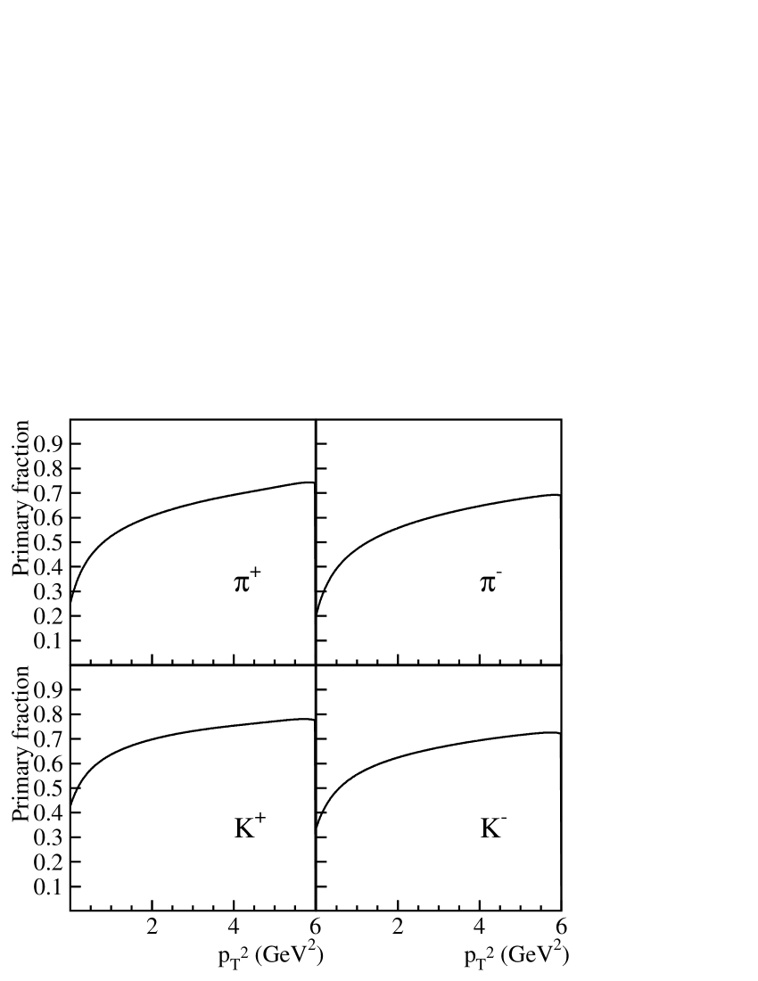
Figure 10: Fraction of primary pions and kaons in pp collisions at $\sqrt{s}=27.4$ GeV estimated by using the fitted parameters in Table 3. The relative primary component increases as a function of $p_{T}^{2}$ but does not reach a value higher than 70-80% even at $p_{T}^{2}$ as high as 6 GeV².

Figure 11: $\chi^{2}$ contour lines in the $T-{\bar{u}}_{T}$ plane for the fits to identified particle transverse momentum spectra in K⁺p collisions at $\sqrt{s}=11.5$ GeV. The contours range from $\chi^{2}_{\rm min}+1$ (1 $\sigma$) to $\chi^{2}_{\rm min}+25$ (5 $\sigma$’s).

Table 4: Particle multiplicities in e⁺e^-collisions.

Particle	Measured	Fitted	Reference
$\sqrt{s}$ = 14 GeV
$\pi^{0}$	4.69 $\pm$ 0.20	4.640	jade
$\pi^{+}$	3.6 $\pm$ 0.3	3.831	tass
K+	0.60 $\pm$ 0.07	0.5872	tass
K${}^{0}_{S}$	0.563 $\pm$ 0.045	0.5557	tass ; jade
p	0.21 $\pm$ 0.03	0.1943	tass
$\Lambda$	0.065 $\pm$ 0.020	0.07972	tass
$\sqrt{s}$ = 22 GeV
$\pi^{0}$	5.5 $\pm$ 0.4	5.488	jade
$\pi^{+}$	4.4 $\pm$ 0.5	4.611	tass
K+	0.75 $\pm$ 0.10	0.6802	tass
K${}^{0}_{S}$	0.638 $\pm$ 0.057	0.6473	tass ; jade
p	0.31 $\pm$ 0.03	0.3012	tass
$\Lambda$	0.110 $\pm$ 0.025	0.1227	tass
$\sqrt{s}$ = 29 GeV
$\pi^{0}$	5.3 $\pm$ 0.7	6.395	tpc
$\pi^{+}$	5.35 $\pm$ 0.25	5.417	tpc
K+	0.70 $\pm$ 0.05	0.7405	tpc
K${}^{0}_{S}$	0.691 $\pm$ 0.029	0.7072	jade ; tpc ; mark2 ; pluto ; hrs
$\eta$	0.584 $\pm$ 0.075	0.5636	mark2 ; hrs
$\rho^{0}$	0.90 $\pm$ 0.05	0.7604	hrs
K∗0	0.281 $\pm$ 0.022	0.2309	tpc ; mark2 ; pluto ; hrs
K∗+	0.310 $\pm$ 0.030	0.2338	tpc
$\eta^{\prime}$	0.26 $\pm$ 0.10	0.05988	mark2
$\phi$	0.084 $\pm$ 0.022	0.08672	tpc
p	0.30 $\pm$ 0.05	0.2812	tpc
$\Lambda$	0.0983 $\pm$ 0.006	0.1023	tpc ; mark2 ; hrs
$\Xi^{-}$	0.0083 $\pm$ 0.0020	0.006844	mark2 ; hrs
$\Sigma^{*+}$	0.0083 $\pm$ 0.0024	0.01030	hrs
$\Omega$	0.0070 $\pm$ 0.0036	0.0004667	mark2
$\sqrt{s}$ = 35 GeV
$\pi^{0}$	6.31 $\pm$ 0.35	6.4786	jade35 ; cello
$\pi^{+}$	5.45 $\pm$ 0.25	5.494	tass35
K+	0.88 $\pm$ 0.10	0.7789	tass35
K${}^{0}_{S}$	0.740 $\pm$ 0.017	0.7444	jade ; cello ; tass
$\eta$	0.636 $\pm$ 0.080	0.5791	jade35 ; cello
$\rho^{0}$	0.756 $\pm$ 0.077	0.7660	tass ; jade35
K∗+	0.361 $\pm$ 0.046	0.2461	tass ; jade35 ; cello
p	0.303 $\pm$ 0.033	0.2900	jade35 ; tass35
$\Lambda$	0.108 $\pm$ 0.010	0.1103	cello ; tass35
$\Xi^{-}$	0.0060 $\pm$ 0.0021	0.007783	tass35
$\sqrt{s}$ = 43 GeV
$\pi^{0}$	6.66 $\pm$ 0.65	6.561	jade35 ; tass35
$\pi^{+}$	5.55 $\pm$ 0.25	5.565	tass35
K+	0.97 $\pm$ 0.15	0.8089	tass43
K${}^{0}_{S}$	0.760 $\pm$ 0.035	0.7735	tass
K∗+	0.385 $\pm$ 0.094	0.2613	tass
$\Lambda$	0.128 $\pm$ 0.024	0.1310	tass35

5.3 Transverse momentum spectra in e⁺e^-collisions

The very definition of transverse momentum spectrum considerably changes from hadronic to e⁺e^-collisions. In the latter, the reference projection axis for $p_{T}$ is no longer the beam line but a suitably defined event or thrust axis, which is the best approximation to the direction of the primarily created q$\bar{\rm q}$ pair. However, this axis has to be determined experimentally on an event by event basis and this is generally done by minimising the sum of tranverse projections of particle momenta. Hence, the transverse momentum of a particle with respect to the event axis is a biased variable in that the same quantity has been used to determine the axis itself. Only when number of particle per event becomes very large, those spurious correlations should be negligible.

Being aware of this difficulty, we have fitted charged particle transverse momentum spectra in e⁺e^-collisions at four different centre-of- mass energies: 14, 22, 29, and 35 GeV eept . Unlike in hadronic collisions, transverse spectra have not been measured for several identified particles and this compelled us to consider only charged tracks. The fit procedure and the treatment of the data was essentially the same as for hadronic collisions except for the preliminary multiplicity fit which has been performed with the old $\gamma_{S}$ parametrisation beca2 instead of the aforementioned (see Subsect. 5.1) new method. Moreover, the hadronic decay chain has been extended to include weak decay products of K${}^{0}_{S}$ and hyperons in order to match the experimental definition of final hadrons in e⁺e^-experiments. The inclusion of heavy flavoured events has been implemented according to the procedure described in ref. beca2 and the branching ratios $R_{q}=\sigma({\rm e}^{+}{\rm e^{-}}\rightarrow q\bar{q})/\sigma_{\rm had}$ have been taken as the lowest order ones $R_{q}\propto Q^{2}_{q}$. Fit results are quoted in Tables 1 and 4.

Figure 12: $\chi^{2}$ contour lines in the $T-{\bar{u}}_{T}$ plane for the fits to charged particle transverse momentum spectra in e⁺e^-collisions at $\sqrt{s}=14,22,29$ and 35 GeV. The contours range from $\chi^{2}_{\rm min}+1$ (1 $\sigma$) to $\chi^{2}_{\rm min}+25$ (5 $\sigma$’s). Also shown the absolute minima and the vertical 1 $\sigma$ temperature band determined by the fit to multiplicities.

The $\chi^{2}$ contour plots in the $T-{\bar{u}}_{T}$ plane are shown in Fig. 12 along with the relevant $1\sigma$ $T_{ch}$ bands. Whilst there is no intersection between best-fit valley and $T_{ch}$ band for e⁺e^-collisions at $\sqrt{s}=14$ GeV, as it was found in K⁺p collisions at $\sqrt{s}=11.5$ GeV, fairly consistent local minima can be determined up to $\sqrt{s}=29$ GeV with sufficiently low ${\bar{u}}_{T}$ values. However, already at $\sqrt{s}=29$ GeV and chiefly at $\sqrt{s}=35$ GeV, the fitted ${\bar{u}}_{T}$ is maybe too large for the assumed zero-order approximation, described in Sect. 3, to hold. This is confirmed by the increasingly high $\chi^{2}$ values demonstrating the inability to fit experimental transverse momentum spectrum to the shape (4). Otherwise stated, as the centre-of-mass energy increases, transverse momentum spectra of hadrons become more and more influenced by the shape (which can no longer be parametrised with an average ${\bar{u}}_{T}$ only) of the transverse four-velocity distribution of hadronising clusters, which is related in turn to the shape of $p_{T}$ distribution of gluons radiated in the perturbative QCD shower. Conversely, the primordial $T$-dependent hadronisation spectrum becomes less and less important; at high energy, its trace is only a small sumperimposed noise smearing out original partonic distributions.

6 Discussion and $m_{T}$ scaling

As has been discussed at the beginning of previous section, two main predictions of the statistical hadronisation model have been provided concerning transverse momentum spectra: the parameters describing the shape of different species should be approximately the same and the extracted temperature should be in agreement with that obtained from fits to average multiplicities.

As far as the latter statement is concerned, a definite answer cannot be given because we have in fact used multiplicity fits to pin down the temperature in spectrum fits. Yet, an independent indication of consistency is provided by the correlation between the temperature location of the global $\chi^{2}$ minima in K⁺p and $\pi^{+}$p collisions at $\sqrt{s}=21.7$ GeV and the corresponding $1\sigma$ band of $T_{ch}$ (see Figs. 7, 8). A clearcut test would be the analysis of spectra with ${\bar{u}}_{T}\simeq 0$, a situation that, in view of the present analysis, is foreseen to occur in a small energy window below $\sqrt{s}\approx 20$ GeV. Focussing solely on the most accurately measured spectra, namely charged pions, it can be seen that ${\bar{u}}_{T}$ appreciably increases from $\sqrt{s}=21.7$ GeV to 27.4 GeV (from 0.12-0.15 to 0.21) whilst $T$ decreases like $T_{ch}$ does, not a surprising fact because the $T_{ch}$ band has been actually used to locate a suitable best-fit value for $T$. On the other hand, if pion spectra are singled out in all three examined collisions, their mimimum $\chi^{2}$ valleys in Figs. 2, 3, 4 nicely overlap and one might be led to argue that, in fact, spectra do no show any significant change of shape from 21.7 to 27.4 GeV. In the assumed statistical formalism, this lack of an observable broadening is due to an accidental compensation between a decrease in temperature and an increase in transverse four-velocity. This effect would be essentially related to a decrease in the chemical temperature $T_{ch}$ from 21.7 to 27.4 GeV and an indication of its physical genuiness would be the apparent correlation between the best-fit global $T$ and $T_{ch}$ band in Figs. 7, 8. However, for the present, such behaviour of temperatures and transverse four-velocities and the possible reason of it cannot be firmly established, as discussed in Subsect. 5.1 with regard to chemical temperature. It might well happen that, resorting to a more fundamental microcanonical description (with hadronisation occurring, for instance, at constant cluster energy density $M/V=$ const), a monotonic evolution of the parameters governing $p_{T}$ and mass slopes as a function of centre-of-mass energy is retrieved while the compensation effect between $T$ and ${\bar{u}}_{T}$ would be only the effect of enforcing a canonical approximation. In general, this topic needs a more detailed study.

Turning back to the first issue, whether statistical parameters describing spectra are sufficiently universal for different hadron species, we have seen in Sect. 5 that rigorous statistical tests would rule out this possibility, though a fully affirmative answer would have indeed been unlikely because of the various approximations inherent to the theoretical formulae. However, the implementation of a single statistical test does not tell us the main sources of the discrepancy between model and data and a further investigation is necessary. As far as pp collisions are concerned, it can be realised by looking at Table 3 and the location of $\chi^{2}$ minimum valleys in Fig. 2, 5, that the different fitted temperatures and tranverse four-velocities are indeed in good agreement with each other with the exception of K⁺ whose spectrum is seemingly harder than expected and significantly different from K^-’s. The $T$ and ${\bar{u}}_{T}$ central values extracted for $\eta$, $\rho^{0}$ and $f_{2}$ are affected by large uncertainties ($\chi^{2}$ minimum valleys are much wider, see Fig. 2) so they are essentially in agreement with the more accurate ones. The situation is slightly worse in the other two examined hadronic collisions, K⁺p and $\pi^{+}$p at $\sqrt{s}=21.7$ GeV. By inspecting Table 3 and Figs. 3, 4, several discrepancies can be noticed: $\pi^{0}$’s spectrum is harder than $\pi^{-}$’s, K${}^{0}_{S}$’s is softer and K^∗’s much too soft; these features are common to both collisions.

Figure 13: Ratio between $m_{T}$ spectra of quoted particles and $\pi^{0}$ spectrum taken as reference for primary (bottom) and final observable hadrons (top) calculated for $T=160$ MeV and ${\bar{u}}_{T}=0.2$ in pp collisions. The spectra have been normalized so as to have the same value at the threshold $m_{T}=m$.

Figure 14: Comparison between experimentally measured $p_{T}^{2}$ and corresponding $m_{T}$ spectra of pions and kaons in pp collisions at $\sqrt{s}=27.4$ GeV. The $p_{T}^{2}$ spectra have been normalized so as to have the same value in the first bin. Lines connecting data points are drawn to guide the eye.

In order to assess the universality as a function of different hadron species, a very useful property is the so-called $m_{T}$-scaling, a well known feature of statistical and thermal models hage ; hage4 : if ${\bar{u}}_{T}=0$, the shape of the primary spectrum of any hadron (except for charged pions at very low $p_{T}$, owing to quantum statistics corrections) depends on its mass only through the variable $m_{T}=\sqrt{p_{T}^{2}+m^{2}}$, as shown in Eq. (4). The $m_{T}$-scaling is broken by a non-vanishing transverse velocity and by the hadronic decay chain but both are small effects for the ${\bar{u}}_{T}$ values found in the present analysis, as it can be seen in Fig. 13: the scaling violation is limited to 25% at the top $m_{T}$ value ($\simeq 2.4$ GeV) in the analysed pp collisions. The general trend of the scaling violation can be roughly summarized with a relative softening of $m_{T}$ spectra of lighter particles with respect to heavier particles.

Figure 15: Ratio between $m_{T}$ spectra of kaons and $\pi^{+}$ spectrum taken as reference. The experimental ratios (dots with error bars) are calculated by using the measured kaon spectra and the fitted $\pi^{+}$ spectrum (parameters quoted in Table 3), which is a very good approximation to the measured one. The theoretical ratios are calculated by taking common values for the relevant parameters, namely $T=160$ MeV and ${\bar{u}}_{T}=0.2$, which are a fair average of values quoted in Table 3. The spectra have been normalized so as to have the same value at the threshold $m_{T}=m_{\rm K}$. Lines connecting data points are drawn to guide the eye.

The approximate $m_{T}$ scaling apparently holds in pp collisions, for the most accurately measured spectra of pions and kaons. That this is a non trivial fact, it is proved in Fig. 14, where the actually measured and published agui91 $p_{T}^{2}$ spectra are compared with the corresponding spectra transformed in the variable $m_{T}$. While $p_{T}^{2}$ slopes are markedly different between pions and kaons, their $m_{T}$ slopes are much closer (heavier particle spectra are affected by too large errors to allow any conclusion). To a closer look, also the aforementioned discrepancy between K⁺ and K^- and the hardness of K⁺ spectrum show up; this is better seen in Fig. 15 where predicted and measured ratios between $m_{T}$ spectra of K⁺ and K^- with respect to $\pi^{+}$’s spectrum are shown. Although the model succeeds in predicting a slight difference between the slopes of K⁺ and K^- (in the right direction) owing to different resonance feeding (the colliding system is not isospin symmetric), the observed ratios with $\pi^{+}$ spectrum are steeper in shape, particularly for K⁺, and the difference between K⁺ and K^- is larger. It is very difficult to understand the reason of this discrepancy; at present, it can attributed to deviations from the model scheme (i.e. from the assumptions listed at the beginning of Sect. 4) or to a systematic error in the estimation of relative abundances of parent hadrons.

Figure 16: Comparison between experimentally measured $p_{T}^{2}$ and corresponding $m_{T}$ spectra of identified particles in K⁺p collisions at $\sqrt{s}=21.7$ GeV. The $p_{T}^{2}$ spectra have been normalized so as to have the same value in the first bin. Lines connecting data points are drawn to guide the eye.

Figure 17: Comparison between experimentally measured $p_{T}^{2}$ and corresponding $m_{T}$ spectra of identified particles in $\pi^{+}$p collisions at $\sqrt{s}=21.7$ GeV. The $p_{T}^{2}$ spectra have been normalized so as to have the same value in the first bin. Lines connecting data points are drawn to guide the eye.

A similar behaviour is observed in K⁺p and $\pi^{+}$p collisions: as shown in Figs. 16, 17, the slopes of $m_{T}$ spectra are definitely much closer than those of $p_{T}^{2}$ spectra. However, in agreement with the previously observed contour plots in Figs. 3, 4 and to the values quoted in Table 3, $\pi^{0}$ spectrum has a remarkably different shape at low $m_{T}$ with respect to $\pi^{-}$’s and K^∗’s spectra are definitely steeper than expected. The softness of K^∗’s spectrum could be related to the presence of a valence strange quark in the initial state for K⁺p collisions; yet it is there in $\pi^{+}$p collisions too. Unfortunately, the spectra in both K⁺p and $\pi^{+}$p collisions have been measured by the same experiment, NA22, and this prevents a cross-check on the data to assess the genuiness of such similarities. Furthermore, there is little overlap between the particle sample in pp and K⁺p, $\pi^{+}$p with the exception of $\pi^{0}$ and $\pi^{-}$. In this regard, whilst in pp collisions very good agreement is found between the measured slopes of the three pion species, a considerable discrepancy is observed in in both K⁺p and $\pi^{+}$p collisions with different initial colliding particles. Indeed, this apparent violation of a nice scaling observed at a centre-of-mass energy only 6 GeV higher is quite odd.

7 Summary and conclusions

Transverse momentum spectra of identified hadrons in several high energy collisions have been compared to the predictions of statistical hadronisation model, which has been described in detail starting from a microcanonical formulation, with emphasis on the assumptions needed to introduce the usual concepts of single-cluster temperature and volume. The distortion effect due to secondary hadronic decays has been accurately and exhaustively taken into account by a newly proposed numerical method. A good agreement is found between model and data and, on top of that, the temperatures estimated by fits to average particle multiplicities and those extracted by fitting transverse momentum spectra are fully compatible with each other. This is an indication in favour of one of the key predictions of the statistical hadronisation model, namely the existence of a close relationship between the production of particles as a function of their mass and, for each particle species, the production as a function of momentum (measured in the rest frame of the cluster they belong to) at the hadronisation.

The model calculations have been performed by taking several assumptions. Firstly, the canonical framework has been used, which is expected to fail at low centre-of-mass energies where the effect of exact transverse momentum conservation must be significant and, in fact, in e⁺e^-collisions at a centre-of-mass energy of 14 GeV and K⁺p collisions at 11.5 GeV, a clear discrepancy between data and calculations shows up. Secondly, the approximation of very small average transverse velocity of the clusters has been introduced, which should break down at high centre-of-mass energy because of the increasingly large $p_{T}$ parton emission (giving rise to clusters with large tranverse velocity). At very high energy, this effect is predominant in determining the shape of transverse momentum spectra whereas hadronisation plays the role of a small superimposed smearing noise. Indeed, it is found that even at moderately high energy e⁺e^-collisions, at $\sqrt{s}=$ 35 GeV, the approximate formulae are no longer able to reproduce the shape of experimental charged particle spectrum and the resulting transverse four-velocity is not consistent with the initial requirement. In summary, the presently used parametrisation of $p_{T}$ spectra is found to work well only in a limited centre-of-mass energy range (roughly between 20 and 30 GeV).

In order to further investigate statistical features of hadronisation, the study of $p_{T}$ spectrum at lower centre-of-mass energy would be greatly interesting but full complex microcanonical calculations are required.

Appendix

Appendix A Proof of the reduction to the EGC

We want to prove by direct transformation that :

$$\Omega=\Big{[}\prod_{i=1}^{N}\sum_{{\bf Q}_{i}}\int{\rm d}^{4}P_{i}\;\theta(P^{0}_{i})\,\Omega_{i}\Big{]}\delta^{4}(P-\Sigma_{i}P_{i})\,\delta_{{\bf Q},\Sigma_{i}{\bf Q}_{i}}$$ (A.1)

is the density of states of an EGC with four-momentum $P=\sum_{i}P_{i}$, quantum numbers ${\bf Q}=\sum_{i}{\bf Q}_{i}$ and volume (in the reference frame where four-momentum is $P$) $V=\sum_{i}V_{i}$. Let us consider the integral representation of Dirac’s and Kronecker’s $\delta$:

$$\!\!\!\!\!\!\delta^{4}(P-\Sigma_{i}P_{i})=\frac{1}{(2\pi)^{4}}\int{\rm d}^{4}x\;{\rm e}^{{\rm i}\,(P-\Sigma_{i}P_{i})\cdot x}$$

$$\!\!\!\!\!\!\delta_{{\bf Q},\Sigma_{i}{\bf Q}_{i}}=\lim_{\mbox{\boldmath${\scriptstyle{\eta}}$}\to 0}\frac{1}{(2\pi)^{n}}\int_{-\mbox{\boldmath${\scriptstyle{\pi}}$}}^{\mbox{\boldmath${\scriptstyle{\pi}}$}}\!\!\!{\rm d}^{n}\phi\;{\rm e}^{{\rm i}({\bf Q}-\Sigma_{i}{\bf Q}_{i})\cdot\mbox{\boldmath${\scriptstyle{\phi}}$}-\Sigma_{i}\mbox{\boldmath${\scriptstyle{\eta}}$}_{i}\cdot{\bf Q}_{i}}$$

where $\mbox{\boldmath$\eta$}=(\eta_{1},\ldots,\eta_{n})$ is a set of real positive numbers which are introduced in order to regularize infinite sums for quantum numbers running from 0 to $+\infty$, such as the absolute number of strange quarks. By using Eq. (A) we can rewrite Eq. (A.1) as:

$$\!\!\!\!\!\!\!\!\!\!\Omega=\frac{1}{(2\pi)^{4+n}}\int{\rm d}^{4}x\int_{-\mbox{\boldmath${\scriptstyle{\pi}}$}}^{\mbox{\boldmath${\scriptstyle{\pi}}$}}\!\!\!{\rm d}^{n}\phi\;{\rm e}^{{\rm i}P\cdot x+{\rm i}{\bf Q}\cdot\mbox{\boldmath${\scriptstyle{\phi}}$}}$$

$$\!\!\!\!\!\!\!\!\!\!\Big{[}\prod_{i=1}^{N}\lim_{\mbox{\boldmath${\scriptstyle{\eta}}$}\to 0}\sum_{{\bf Q}_{i}}\int{\rm d}^{4}P_{i}\;{\rm e}^{-{\rm i}P_{i}\cdot x-{\rm i}{\bf Q}_{i}\cdot\mbox{\boldmath${\scriptstyle{\phi}}$}-\mbox{\boldmath${\scriptstyle{\eta}}$}_{i}\cdot{\bf Q}_{i}}\,\theta(P^{0}_{i})\,\Omega_{i}\Big{]}$$ (A.3)

Let us focus on the single $i^{\rm th}$ factor in the above product. If one plugs in it the expression (6) of $\Omega_{i}$ and the $\theta$ function’s integral representation:

$$\theta(P^{0}_{i})=\frac{1}{2\pi{\rm i}}\int_{-\infty-{\rm i}\varepsilon}^{+\infty-{\rm i}\varepsilon}\!\!\!\!\!\!\!\!\!\!{\rm d}\alpha\;\frac{{\rm e}^{{\rm i}\alpha P^{0}_{i}}}{\alpha}$$ (A.4)

the following expression is obtained:

$$\lim_{\mbox{\boldmath${\scriptstyle{\eta}}$}\to 0}\frac{1}{2\pi{\rm i}}\sum_{{\bf Q}_{i}}\int{\rm d}^{4}P_{i}\int_{-\infty-{\rm i}\varepsilon}^{+\infty-{\rm i}\varepsilon}\!\!\!\!\!\!\!\!\!\!{\rm d}\alpha\int{\rm d}^{4}x_{i}\int_{-\mbox{\boldmath${\scriptstyle{\pi}}$}}^{\mbox{\boldmath${\scriptstyle{\pi}}$}}\!\!\!{\rm d}^{n}\phi_{i}\;$$

$$\frac{{\rm e}^{{\rm i}\alpha P^{0}_{i}-{\rm i}P_{i}\cdot(x-x_{i})-{\rm i}{\bf Q}_{i}\cdot(\mbox{\boldmath${\scriptstyle{\phi}}$}-\mbox{\boldmath${\scriptstyle{\phi}}$}_{i})-\mbox{\boldmath${\scriptstyle{\eta}}$}_{i}\cdot{\bf Q}_{i}}}{\alpha}\,{\rm e}^{F(x_{i},\mbox{\boldmath${\scriptstyle{\phi}}$}_{i})}$$ (A.5)

where the limit $\mbox{\boldmath$\eta$}\rightarrow 0$ is implied. The integration in $P_{i}$ in Eq. (A) formally (that is, in a distributional sense) yields $(2\pi)^{4}\delta(x^{0}_{i}-x^{0}+\alpha)\delta^{3}({\bf x}_{i}-{\bf x})$. On the other hand, the sum over the quantum number vectors ${\bf Q}_{i}$ yields, for its generic $k^{\rm th}$ component:

$$\!\!\!\!\!\!\!\!\!\!\!\!2\pi\delta(\phi_{k}-\phi_{ik})\qquad{\rm if}\;\;Q_{ik}=-\infty,\ldots,+\infty$$

$$\!\!\!\!\!\!\!\!\!\!\!\!\lim_{\eta_{k}\to 0}\frac{1}{1-\exp[{\rm i}(\phi_{ik}-\phi_{k})-\eta_{k}]}\qquad{\rm if}\;\;Q_{ik}=0,\ldots,+\infty$$

In fact, the second expression in the above equation is also equivalent to a $\delta$ distribution. This can be shown through a transformation of the integration in $\phi_{i}$ over the interval $(-\pi,\pi)$ onto the unitary circle in the complex plane by setting $w=\exp[-{\rm i}\phi_{ik}]$:

$$\lim_{\eta_{k}\to 0}\int_{-\pi}^{\pi}\!\!\!{\rm d}\phi_{ik}\;\frac{1}{1-\exp[{\rm i}(\phi_{ik}-\phi_{k})-\eta_{k}]}\,{\rm e}^{F(x_{i},\mbox{\boldmath${\scriptstyle{\phi}}$}_{i})}$$

$$=\lim_{\eta_{k}\to 0}\frac{1}{{\rm i}}\oint{\rm d}w\;\frac{\exp[F_{w}(x_{i},\phi_{1},\ldots,w,\ldots,\phi_{n})]}{w-{\rm e}^{-{\rm i}\phi_{k}-\eta_{k}}}$$ (A.7)

The function $F_{w}$ (see Eq. (2.1)) is analytic with respect to the complex variable $w$ as only positive integer powers of $w$ are involved (the $q_{kj}$’s are positive integer numbers by assumption) and the pole ${\rm e}^{-{\rm i}\phi_{k}-\eta_{k}}$ lies within the unitary circle. Thus, the result of the integral in Eq. (A) is simply:

$$\lim_{\eta_{k}\to 0}2\pi\exp[F_{w}(x_{i},\phi_{i1},\ldots,{\rm e}^{-{\rm i}\phi_{k}-\eta_{k}},\ldots,\phi_{in})]$$

$$= 2\pi\exp[F(x_{i},\phi_{i1},\ldots,\phi_{k},\ldots,\phi_{in})]$$ (A.8)

which is the same result that would have been obtained by integrating with a $\delta$ distribution. Of course, the same procedure may be repeated for all components other than $k$. Eventually, the integrations in $x_{i}$ and $\mbox{\boldmath$\phi$}_{i}$ in (A) yield:

$$\lim_{\varepsilon\to 0}\frac{1}{2\pi{\rm i}}\int_{-\infty-{\rm i}\varepsilon}^{+\infty-{\rm i}\varepsilon}\!\!\!\!\!\!\!\!\!\!{\rm d}\alpha\;\frac{\exp[F(x^{0}-\alpha,{\bf x},\mbox{\boldmath$\phi$})]}{\alpha}$$ (A.9)

This integral can be calculated by closing the $z=-{\rm i}\varepsilon$ line with a semicircle lying in the upper half of the complex plane and taking the limit for the circle radius going to infinity. Since the function $F$ is analytic with respect to $\alpha$ (see Eq. (2.1)), the result is simply:

$$\exp[F(x^{0},{\bf x},\mbox{\boldmath$\phi$})]=\exp[F(x,\mbox{\boldmath$\phi$})]$$ (A.10)

which is the final form of expression (A). Now the function $F$ depends on the particular $i^{\rm th}$ cluster only through the volume $V_{i}$ with a simple linear relationship, namely $F(x,\mbox{\boldmath$\phi$})\equiv V_{i}f(x,\mbox{\boldmath$\phi$})$ (see Eq. (2.1)). Therefore, the product of all the factors (A) yields:

$$\exp[\sum_{i}V_{i}f(x,\mbox{\boldmath$\phi$})]$$ (A.11)

and this is the final form of the expression between square brackets in Eq. (A). Hence, the $\Omega$ function reads:

$$\Omega=\frac{1}{(2\pi)^{4+n}}\int{\rm d}^{4}x\int_{-\mbox{\boldmath${\scriptstyle{\pi}}$}}^{\mbox{\boldmath${\scriptstyle{\pi}}$}}\!\!\!{\rm d}^{n}\phi\;{\rm e}^{{\rm i}P\cdot x+{\rm i}{\bf Q}\cdot\mbox{\boldmath${\scriptstyle{\phi}}$}}\,{\rm e}^{(\Sigma_{i}V_{i})f(x,\mbox{\boldmath${\scriptstyle{\phi}}$})}$$ (A.12)

QED.

Appendix B Decomposition of Lorentz transformations

A general Lorentz transformation ${\sf\Lambda}$ can be uniquely decomposed as the product of a transformation like in Eq. (42) and a general rotation group :

$${\sf\Lambda}={\sf L}{\sf R}\qquad{\sf L}={\sf\hat{R}}_{3}(\varphi)\,{\sf\hat{R}}_{2}(\theta)\,{\sf\hat{L}}_{3}(\xi)$$ (B.1)

where $\varphi\in[0,2\pi)$, $\theta\in[0,\pi]$ and $\xi\geq 0$ (see Eq. (42)).
Any timelike vector can be uniquely written as ${\sf L}(\hat{t})$ where $\hat{t}=(1,0,0,0)$ is the time axis unit vector and ${\sf L}$ like in Eqs. (42,B.1) group . Hence, given two timelike vectors $P^{\prime}={\sf L}^{\prime}(\hat{t})$ and $P={\sf L}(\hat{t})$ there is only one Lorentz transformation of the type (42,B.1) transforming $P^{\prime}$ into $P$, namely ${\sf L}^{\prime\prime}$ such that ${\sf L}^{\prime\prime}(\hat{t})={\sf L}{\sf L}^{\prime-1}(\hat{t})$.

In order to prove the alternative decomposition of ${\sf L}$ in Eq. (78), it is sufficient to show that the equation:

$${\sf\hat{R}}_{3}(\varphi)\,{\sf\hat{R}}_{2}(\theta)\,{\sf\hat{L}}_{3}(\xi)(\hat{t})={\sf\hat{L}}_{3}(\eta)\,{\sf\hat{R}}_{3}(\phi)\,{\sf\hat{L}}_{1}(\zeta)(\hat{t})$$ (B.2)

with $\phi\in[0,2\pi)$, $\eta\in(-\infty,+\infty)$ and $\zeta\geq 0$, establishes a biunivocal correspondance between the two sets of coordinates. Eq. (B.2) leads to the system of equations:

$$\cosh\zeta\cosh\eta = \cosh\xi$$

$$\sinh\zeta\cos\phi = \sinh\xi\sin\theta\cos\varphi$$

$$\sinh\zeta\sin\phi = \sinh\xi\sin\theta\sin\varphi$$

$$\cosh\zeta\sinh\eta = \sinh\xi\cos\theta$$ (B.3)

whose solution is:

$$\cosh\xi = \cosh\zeta\cosh\eta$$

$$\tan\theta = \frac{\tanh\zeta}{\sinh\eta}$$

$$\varphi = \phi$$ (B.4)

and its inverse:

$$\cosh\eta = \frac{\cosh\xi}{\sqrt{1+\sinh^{2}\xi\sin^{2}\theta}}$$

$$\sinh\zeta = \sinh\xi\sin\theta$$

$$\phi = \varphi$$ (B.5)

Therefore, if Eq. (42) is a valid decomposition, Eq. (78) holds as well, within the relevant variable domains.

The associated invariant measure in the variables $\zeta$, $\eta$ and $\phi$ can be obtained by calculating the jacobian of the transformation (B) and taking into account that ${\rm d}{\sf L}=\sinh^{2}\xi\,\sin\theta\,{\rm d}\xi\,{\rm d}\theta\,{\rm d}\varphi$ group2 . It is advantegeous to rewrite the above measure as ${\rm d}{\sf L}=\sinh\xi\,{\rm d}\cosh\xi\,{\rm d}\cos\theta\,{\rm d}\varphi$ and use the following transformation formulae derived by Eqs. (B) and (B):

$$\cosh\xi = \cosh\zeta\cosh\eta$$

$$\cos\theta = \frac{\cosh\zeta\sinh\eta}{\sqrt{\cosh^{2}\zeta\cosh^{2}\eta-1}}$$

implying:

$$|\det J|=\frac{\cosh\zeta\sinh\zeta}{\sqrt{\cosh^{2}\zeta\cosh^{2}\eta-1}}$$

and, consequently:

$${\rm d}{\sf L}=\frac{\sinh 2\zeta}{2}\,{\rm d}\zeta\,{\rm d}\eta\,{\rm d}\phi$$ (B.6)

Appendix C Calculation of the secondary contribution to transverse momentum spectrum

The integration of Eq. (4) is performed by solving the $\delta$ function with respect to the $\varphi$ azimuthal angle according to the well known formula:

$$\delta(f(\varphi))=\sum_{i}\frac{1}{|f^{\prime}(\varphi_{0i})|}\delta(\varphi-\varphi_{0i})$$ (C.1)

where $\varphi_{0i}$ are the zeroes of the $f$ function. In the present case (see Eq. (111)):

$$f(\varphi)=x-{\bar{\gamma}}_{T}\epsilon-{\bar{u}}_{T}p_{T}\cos\varphi$$ (C.2)

thus:

$$\cos\varphi_{0}=\frac{{\bar{\gamma}}_{T}\epsilon-x}{{\bar{u}}_{T}p_{T}}$$ (C.3)

$$|f^{\prime}(\varphi_{0})|={\bar{u}}_{T}p_{T}\sqrt{1-\cos^{2}\varphi_{0}}$$

There are two angles fulfilling Eq. (C.3) in the $[0,2\pi)$ interval, provided that the absolute value of its right hand side is $<1$. For these angles, the absolute value of the derivatives in the lower equation are equal. Hence, the integration in Eq. (4) in the azimuthal angle yields 2 if $|{\bar{\gamma}}_{T}\epsilon-x|<{\bar{u}}_{T}p_{T}$ and 0 otherwise. Therefore, Eq. (4) turns into:

$$\Big{\langle}\frac{{\rm d}n}{{\rm d}p_{T}}\Big{\rangle}^{k\rightarrow j}\!\!\!\!=2\int_{m_{j}}^{+\infty}\!\!\!\!{\rm d}x\int_{-\infty}^{+\infty}\!\!\!\!{\rm d}p_{z}\;\frac{p_{T}}{4\pi\epsilon\sqrt{x^{2}-m_{j}^{2}}}\,\Big{\langle}\frac{{\rm d}n}{{\rm d}\epsilon^{*}}\Big{\rangle}^{k\rightarrow j}\!\!\!\!\!\!(x)\,$$

$$\times\frac{\theta({\bar{u}}_{T}p_{T}-|{\bar{\gamma}}_{T}\epsilon-x|)}{\sqrt{\overline{u_{T}^{2}}p_{T}^{2}-({\bar{\gamma}}_{T}\epsilon-x)^{2}}}$$ (C.4)

The next integration can be done with the change of variable $p_{z}=m_{T}\sinh y$, i.e. by introducing rapidity, so that $\epsilon=m_{T}\cosh y$ and Eq. (C) reads:

$$\Big{\langle}\frac{{\rm d}n}{{\rm d}p_{T}}\Big{\rangle}^{k\rightarrow j}\!\!\!\!=4\int_{m_{j}}^{+\infty}\!\!\!\!{\rm d}x\int_{0}^{+\infty}\!\!\!\!{\rm d}y\;\frac{p_{T}}{4\pi\sqrt{x^{2}-m_{j}^{2}}}\,\Big{\langle}\frac{{\rm d}n}{{\rm d}\epsilon^{*}}\Big{\rangle}^{k\rightarrow j}\!\!\!\!\!\!(x)\,$$ (C.5)

$$\times\frac{\theta({\bar{u}}_{T}p_{T}-|{\bar{\gamma}}_{T}m_{T}\cosh y-x|)}{\sqrt{\overline{u_{T}^{2}}p_{T}^{2}-({\bar{\gamma}}_{T}m_{T}\cosh y-x)^{2}}}$$

where advantage has been taken of the fact that the integrand is even in rapidity. The last needed change of variable is $z=\cosh y$, leading to:

$$\Big{\langle}\frac{{\rm d}n}{{\rm d}p_{T}}\Big{\rangle}^{k\rightarrow j}\!\!\!\!=4\int_{m_{j}}^{+\infty}\!\!\!\!{\rm d}x\int_{1}^{+\infty}\!\!\!\!{\rm d}z\;\frac{p_{T}}{4\pi\sqrt{x^{2}-m_{j}^{2}}}\,\Big{\langle}\frac{{\rm d}n}{{\rm d}\epsilon^{*}}\Big{\rangle}^{k\rightarrow j}\!\!\!\!\!\!(x)\,$$

$$\times\frac{\theta(z-z_{-})\theta(z_{+}-z)}{{\bar{\gamma}}_{T}m_{T}\sqrt{(z-1)(z+1)(z-z_{-})(z_{+}-z)}}$$ (C.6)

where $z_{+}$ and $z_{-}$ are defined in Eq. (4) and, obviously, ${\bar{\gamma}}_{T}=\sqrt{1+\overline{u_{T}^{2}}}$. The integral in the $z$ variable is an elliptic integral whose solutions depend on the sign of $z_{-}-1$; they can be found in ref. grads :

$$\int_{1}^{+\infty}\!\!\!\!{\rm d}z\;\frac{\theta(z-z_{-})\theta(z_{+}-z)}{\sqrt{(z-1)(z+1)(z-z_{-})(z_{+}-z)}}=$$

$$=\frac{2}{\sqrt{(z_{+}-z_{\rm min})(z_{\rm max}+1)}}\;{\rm F}\left(\frac{\pi}{2},r\right)$$ (C.7)

where $z_{\rm min}$, $z_{\rm max}$ and $r$ are quoted in Eq. (4) and F is the complete elliptic integral of the first kind. After the substitution of $x$ with momentum ${\rm p}^{*}=\sqrt{x^{2}-m_{j}^{2}}$ as integration variable in Eq. (C), the final result is exactly as in Eq. (4).

Appendix D Calculation of the partition function with fixed number of strange quarks

In this section we describe the technique used to handle the numerical integration of canonical partition functions with four fixed quantum numbers, namely electric charge $Q$, baryon number $B$, strangeness $S$ and number of ${\rm s}+\bar{\rm s}$ quarks $N_{S}$. This can be written as in Eq. (101) with $n=4$ and $\lambda_{j}=1$:

$$Z({\bf Q})=\frac{1}{(2\pi)^{4}}\int_{-\mbox{\boldmath${\scriptstyle{\pi}}$}}^{\mbox{\boldmath${\scriptstyle{\pi}}$}}\!\!\!{\rm d}^{4}\phi\;\exp\,[{\rm i}{\bf Q}\cdot\mbox{\boldmath$\phi$}+F_{\rm c}(\mbox{\boldmath$\phi$})]$$ (D.1)

with ${\bf Q}=(Q,B,S,N_{S})$ and:

$$F_{\rm c}(\mbox{\boldmath$\phi$})=\frac{\overline{V}}{(2\pi)^{3}}\!\sum_{j}(2J_{j}+1)\!\int\!{\rm d}^{3}{\rm p}\;\log\,[1\pm{\rm e}^{-\varepsilon_{j}/T-{\rm i}{\bf q}_{j}\cdot\mbox{\boldmath${\scriptstyle{\phi}}$}}]^{\pm 1}$$ (D.2)

Straight numerical four-dimensional integration is too time consuming to allow reasonably quick multiplicity fits: an analytical reduction of the above integral is indeed necessary. For this purpose, we first integrate out the $\phi_{B}$ variable associated with baryon number. This can be done analitically because of the presence of only single-valued baryons in the function $F_{\rm c}$ in Eq. (D.1), neglecting the corrections due to Fermi statistics which are very small. Thus:

$$F_{\rm c}(\mbox{\boldmath$\phi$})=F_{\rm c}(\phi_{Q},\phi_{S},\phi_{N_{S}})_{\rm mesons}+W_{+}{\rm e}^{-{\rm i}\phi_{B}}+W_{-}{\rm e}^{{\rm i}\phi_{B}}$$ (D.3)

where:

$$W_{\pm}=\sum_{\rm bar.\atop antibar.}z_{j}\exp\,[-{\rm i}(Q_{j}\phi_{Q}+S_{j}\phi_{S}+N_{Sj}\phi_{N_{S}})]$$ (D.4)

$$z_{j}\equiv\frac{\overline{V}(2J_{j}+1)}{(2\pi)^{3}}\int{\rm d}^{3}{\rm p}\;\exp\,[-\varepsilon_{j}/T]$$ (D.5)

It must be stressed that $W_{+}\neq W^{*}_{-}$ because the number of strange quarks is the same for both particles and antiparticles. The integration in $\phi_{B}$ in Eq. (D.1) can be performed by using the decomposition (D.3) and a series is obtained:

$$\frac{1}{2\pi}\!\!\int_{-\pi}^{\pi}\!\!\!{\rm d}\phi_{B}\;{\rm e}^{{\rm i}B\phi_{B}}\exp\,[W_{+}{\rm e}^{-{\rm i}\phi_{B}}+W_{-}{\rm e}^{{\rm i}\phi_{B}}]\!=\!\!\sum_{k=0}^{\infty}\frac{W_{+}^{k+B}W_{-}^{k}}{k!(k+B)!}$$ (D.6)

Then, the integration in $\phi_{N_{S}}$ in Eq. (D.1) is performed. It is advantegeous to set $w=\exp[-{\rm i}\phi_{N_{S}}]$ and map the interval $[-\pi,\pi)$ onto the unitary circle in the complex plane:

$$\frac{1}{2\pi{\rm i}}\oint\frac{{\rm d}w}{w}\;w^{-{N_{S}}}\Sigma(w)\exp[{\tilde{F}}_{\rm M}(w)]$$ (D.7)

where:

$${\tilde{F}}_{\rm M}(w)=F_{\rm c}(\phi_{Q},\phi_{S},\phi_{N_{S}})_{\rm mesons}$$ (D.8)

and $\Sigma$ is the series in Eq. (D.6). Since mesons can contain at most two strange quarks, the function ${\tilde{F}}_{\rm M}(w)$ can be written as the sum of three terms:

$${\tilde{F}}_{\rm M}(w)=\alpha+\beta w+\gamma w^{2}$$ (D.9)

where $\alpha$, $\beta$ and $\gamma$ are the sums $\Sigma_{j}z_{j}\exp\,[-{\rm i}Q_{j}\phi_{Q}-{\rm i}S_{j}\phi_{S}]$ over mesons with 0, 1 and 2 strange quarks respectively. As baryons may contain at most three strange quarks, the functions $W_{+}(w)$ and $W_{-}(w)$ in (D.4) are third-degree polynomials in $w$ with conjugate coefficients $A_{0},\ldots,A_{3}$ depending on $\phi_{Q}$ and $\phi_{S}$, i.e.:

$$W_{+}(w)=\sum_{n=1}^{3}A_{n}w^{n}\qquad W_{-}(w)=\sum_{n=1}^{3}A^{*}_{n}w^{n}$$ (D.10)

and, consequently, the series $\Sigma(w)$ in Eq. (D.6) is an analytic function of $w$. Hence, the integrand in Eq. (D.7) has one pole of $N_{S}^{\rm th}$ order in $w=0$ and the integral (D.7) turns out to be:

$$\frac{\exp[\alpha]}{N_{S}!}\frac{{\rm d}^{N_{S}}}{{\rm d}z^{N_{S}}}\exp\,[\beta w+\gamma w^{2}]\Sigma(w)\Big{|}_{w=0}$$ (D.11)

The derivative can be calculated along any direction and particularly along the real axis. Finally, the partition function in Eq. (D.1) reads:

$$Z({\bf Q})=\frac{1}{(2\pi)^{2}}\int_{-\pi}^{\pi}\!\!\!{\rm d}\phi_{Q}\int_{-\pi}^{\pi}\!\!\!{\rm d}\phi_{S}\;{\rm e}^{{\rm i}Q\phi_{Q}+iS\phi_{S}+\alpha(\phi_{Q},\phi_{S})}$$

$$\times\frac{{\rm D}^{N_{S}}\Sigma(x)\exp\,[\beta(\phi_{Q},\phi_{S})x+\gamma(\phi_{Q},\phi_{S})x^{2}]|_{x=0}}{N_{S}!}$$ (D.12)

which is to be integrated numerically within its two dimensional domain.
The next problem is how to calculate the derivative in the integrand in Eq. (D). We first notice that the series $\Sigma$ can be calculated analytically for a real argument because $W_{+}(x)=W^{*}_{-}(x)$ (see Eq. (D.10)):

$$\Sigma(x) = \sum_{k=0}^{\infty}\frac{W_{+}(x)^{k+B}W^{*}_{+}(x)^{k}}{k!(k+B)!}$$ (D.13)

$$= {\rm I}_{B}(2|W_{+}(x)|)\exp\,[{\rm i}B\arg W_{+}(x)]$$

$$= \frac{{\rm I}_{B}(2|W_{+}(x)|)}{(2|W_{+}(x)|)^{B}}\,(2W_{+}(x))^{B}$$

where ${\rm I}_{B}$ is the modified Bessel function of order $B$. The derivative of order ${N_{S}}$ is then expanded:

$${\rm D}^{N_{S}}\Sigma(x)\exp\,[\beta x+\gamma x^{2}]=$$

$$=\sum_{k=0}^{N_{S}}{N_{S}\choose k}{\rm D}^{k}\exp\,[\beta x+\gamma x^{2}]{\rm D}^{N_{S}-k}\Sigma(x)$$ (D.14)

It can be shown with a little algebra that:

$${\rm D}^{k}\exp[\beta x+\gamma x^{2}]\Big{|}_{x=0}=k!\sum_{j\geq k/2}^{k}\frac{\beta^{2j-k}\gamma^{k-j}}{(2j-k)!(k-j)!}$$ (D.15)

The derivative of $\Sigma(x)$ can be further expanded:

$${\rm D}^{k}\Sigma(x)=\sum_{l=0}^{k}{k\choose l}{\rm D}^{l}\frac{{\rm I}_{B}(2|W_{+}(x)|)}{(2|W_{+}(x)|)^{B}}\,{\rm D}^{k-l}(2W_{+}(x))^{B}$$ (D.16)

The derivative of the first factor in the above sum can be calculated by taking advantage of recurrence relations for Bessel function derivatives:

$${\rm D}\frac{{\rm I}_{B}(2|W_{+}(x)|)}{(2|W_{+}(x)|)^{B}}=\frac{{\rm I}_{B+1}(2|W_{+}(x)|)}{(2|W_{+}(x)|)^{B+1}}\,\,2\,{\rm D}|W_{+}(x)|^{2}$$ (D.17)

while for the second factor:

$${\rm D}(2W_{+}(x))^{B}=B(2W_{+}(x))^{B-1}\,{\rm D}W_{+}(x)$$ (D.18)

The two equations above are the starting point for the numerical calculation of the derivative in Eq. (D.16); a recursive algorithm has been implemented that computes it for $x=0$, taking into account that (see Eq. (D.10)):

$$\frac{{\rm I}_{B}(2|W_{+}(0)|)}{(2|W_{+}(0)|)^{B}}=\frac{{\rm I}_{B}(2|A_{0}|)}{(2|A_{0}|)^{B}}$$

$${\rm D}^{l}|W_{+}(x)|^{2}\Big{|}_{x=0}=l!\sum_{n=0}^{l}A_{n}A^{*}_{l-n}$$

$${\rm D}^{l}W_{+}(x)\Big{|}_{x=0}=l!\,A_{l}$$

References

• (1) E. Fermi, Progr. Theor. Phys. 5 (1950) 570.
• (2) R. Hagedorn, N. Cim. Suppl. 3 (1965) 147.
• (3) F. Becattini, Z. Phys. C 69 (1996) 485.
• (4) F. Becattini, Proc. of XXXIII Eloisatron Workshop on ”Universality Features in Multihadron Production and the leading effect” (1996) 74, hep-ph 9701275.
• (5) F. Becattini and U. Heinz, Z. Phys. C 76 (1997) 269.
• (6) U. Heinz, Nucl. Phys. A 661 (1999) 140.
• (7) R. Stock, Phys. Lett. B 456 (1999) 277.
• (8) R. Hagedorn, CERN lectures ”Thermodynamics of strong interactions” (1970) 46.
• (9) R. Hagedorn, ”Hot Hadronic Matter: Theory and Experiment” (1994) 13 and references therein.
• (10) R. Hagedorn, Riv. N. Cim. 6 (1984) 1983.
• (11) J. Sollfrank, P. Koch and U. Heinz, Phys. Lett. B 252 (1990) 256.
• (12) J. Sollfrank, P. Koch and U. Heinz, Z. Phys. C 52 (1991) 593.
• (13) U. A. Wiedemann and U. Heinz, Phys. Rev. C 56 (1997) 3265.
• (14) T. Peitzmann, Nucl. Phys. A 638 (1998) 415c.
• (15) G. Marchesini and B. Webber, Nucl. Phys. B 238 (1984) 1.
• (16) for a description of the model in the canonical approximation see F. Becattini, Proc. of XI Chris Engelbrecht summer school ”Hadrons in dense matter and hadrosynthesis” (1998) 71.
• (17) W. K. Tung, ”Group Theory in Physics”, World Scientific, Singapore.
• (18) W. Ruhl, ”The Lorentz group and harmonic analysis”, W. A. Benjamin, New York 1970.
• (19) T. Sjöstrand, ”PYTHIA 5.7 and JETSET 7.4 Physics and Manual”, CERN-TH 7112/93; T. Söstrand, Comp. Phys. Comm. 82 (1994) 74.
• (20) C. Caso et al., ”The Review of Particle Physics 1998”, Eur. Phys. J. C 3 (1998) 1.
• (21) Routine HQUAD of the package HBOOK, CERN program library long writeup Y250.
• (22) P. V. Chliapnikov, private communication.
• (23) M. Aguilar-Benitez et al., Z. Phys. C 50 (1990) 405.
• (24) M. Barth et al., Z. Phys. C 22 (1984) 23.
• (25) M. Barth. et al., Z. Phys. C 7 (1981) 187.
• (26) M. Barth et al., Nucl. Phys. B 223 (1983) 296, Erratum-ibid. B 232 (1984) 547.
• (27) M. Barth et al., Z. Phys. C 10 (1981) 205, Erratum-ibid. C 11 (1981) 271.
• (28) M. Barth et al., preprint IFVE-82-144 (1982).
• (29) M. Adamus et al., Z. Phys. C 32 (1986) 475.
• (30) M. R. Atayan et al., Z. Phys. C 54 (1992) 247.
• (31) I. V. Azhinenko et al., Z. Phys. C 46 (1990) 525.
• (32) N. M. Agababian et al., Z. Phys. C 41 (1989) 539.
• (33) I.V. Azhinenko et al., Z. Phys. C 44 (1989) 573.
• (34) N. M. Agababyan et al., Z. Phys. C 46 (1990) 387.
• (35) H. Kichimi et al., Phys. Rev. D 20 (1979) 37.
• (36) R. D. Kass et al., Phys. Rev. D 20 (1979) 605.
• (37) A. Suzuki et al., Nucl. Phys. B 172 (1980) 327.
• (38) F. Becattini, M. Gazdzicki, J. Sollfrank, Eur. Phys. J. C 5 (1998) 143.
• (39) M. I. Gorenstein, M. Gazdzicki, W. Greiner, Phys. Lett. B 483 (2000) 60.
• (40) B. P. Roe, ”Probability and Statistics in Experimental Physics”, Springer-Verlag 1992.
• (41) I. V. Azhinenko et al., Z. Phys. C 35 (1987) 7.
• (42) M. Adamus et al., Z. Phys. C 39 (1988) 311.
• (43) A. Suzuki et al., Lett. N. Cim. 24 (1979) 31.
• (44) ”MINUIT - Function minimisation and error analysis”, CERN program library long writeup D506.
• (45) M. Barth et al., Z. Phys. C 22 (1985) 23.
• (46) M. Barth et al., Nucl. Phys. B 191 (1981) 39.
• (47) JADE coll., Z. Phys. C 28 (1985) 343; Z. Phys. C 20 (1985) 187.
• (48) TASSO coll., Z. Phys. C 27 (1985) 27; Z. Phys. C 47 (1990) 167.
• (49) TPC coll., Z. Phys. C 27 (1985) 187; Phys. Lett. B 184 (1987) 299; Phys. Rev. Lett. 53 (1984) 2378; Phys. Rev. Lett. 54 (1985) 274; Phys. Rev. Lett. 52 (1984) 2201.
• (50) MARK-II coll., Phys. Rev. D 31 (1985) 3013; Phys. Rev. Lett. 61 (1988) 1057; Phys. Rev. Lett. 54 (1986) 2071; Phys. Rev. Lett. 58 (1987) 644; Phys. Rev.Lett. 59 (1987) 2412.
• (51) PLUTO coll., Phys. Lett. B 104 (1981) 79.
• (52) HRS coll., Phys. Rev. D 41 (1990) 2045; Phys. Lett. B 205 (1987) 111; Phys. Rev. D 40 (1989) 706; Phys. Rev. D 45 (1992) 3949; Phys. Rev. Lett. 58 (1987) 2627.
• (53) JADE coll., Z. Phys. C 46 (1990) 1; Phys. Lett. B 145 (1984) 441; Phys. Lett. B 104 (1981) 325.
• (54) CELLO coll., Z. Phys. C 47 (1990) 1; Z. Phys. C 46 (1990) 397.
• (55) TASSO coll., Z. Phys. C 42 (1989) 189; Z. Phys. C 45 (1989) 209.
• (56) TASSO coll., Z. Phys. C 45 (1989) 193.
• (57) TASSO coll., Z. Phys. C 22 (1984) 307; HRS coll., Phys. Rev. D 31 (1985) 1; TASSO coll., Z. Phys. C 47 (1990) 187.
• (58) The Durham reaction data database, web address: http://durpdg.dur.ac.uk/HEPDATA/REAC
• (59) I. S. Gradshteyn, I. M. Ryzhik, ”Table of integrals, series and products”, $6^{\rm th}$ edition, Ed. A. Jeffrey, Academic Press 2000, p. 272.