Phenomenology from Lattice QCD

Abstract

I review two subjects in which lattice simulations are making, or can make in the future, a significant contribution to particle physics phenomenology. The first subject is the evaluation of quantities which enter into the determination of the vertex $A$ of the unitarity triangle from experimental measurements of decay rates and mixing amplitudes. These quantities include the form-factors for semileptonic $B$-decays, the leptonic decay constants of the $B$ and $B_{s}$ mesons and the $B$-parameters for $B_{d}$-$\bar{B}_{d}$ and $B_{s}$-$\bar{B}_{s}$ mixing and the corresponding parameter for $K$-$\bar{K}$ mixing, $B_{K}$. In the second part of this talk I will review the status and prospects for the evaluation of $K\to\pi\pi$ amplitudes and for the subsequent study of the $\Delta I=1/2$ rule and the evaluation of $\varepsilon^{\prime}/\varepsilon$.

1 Introduction

In this lecture I will briefly review some of the contributions which lattice computations are making to particle physics phenomenology. The lattice formulation of quantum field theory together with large-scale numerical simulations is contributing to a wide variety of fundamental questions in particle physics, both theoretical and phenomenological. Here I will concentrate on one of the most important rôles of lattice QCD, the evaluation of non-perturbative QCD effects in physical amplitudes and other quantities. Indeed, it is frequently our inability to quantify the long-distance QCD effects in weak processes which is the dominant source of uncertainty in determining fundamental quantities from experimental measurements and lattice simulations provide an ab initio framework for the evaluation of these effects.

For many physical quantities lattice calculations have been performed for over ten years and the emphasis is on the reduction of systematic uncertainties. I will briefly outline the sources of some of the other uncertainties when presenting the results below, but let me now mention two important sources of error which the community is striving to reduce. The first of these is quenching, the neglect of vacuum polarization and other quark loop-effects. Most large-scale phenomenological calculations have been performed in the quenched approximation, although increasingly calculations are being performed with 2 flavours of sea quarks. Although it is natural to be skeptical about quenched calculations and consider full QCD (unquenched) ones as totally reliable, in my opinion neither of these views is fully justified at present. Where results from quenched calculations can be compared with experimental measurements, they typically agree to within 10% or so, which is sufficiently accurate for some quantities and not so for others. On the other hand, it should also be remembered that in unquenched simulations the masses of the sea and valence quarks are large ($m_{\pi}/m_{\rho}$ is typically about 0.6 or more) so that significant extrapolations are needed, and this also leads to uncertainties. This brings me to the second source of lattice systematic error, which is increasingly being studied in detail, the extrapolation to the chiral limit. In order to avoid unphysical effects due to the finite volume of the lattice, simulations are performed with up and down quarks with masses ($m_{u}$ and $m_{d}$) in the region of $m_{s}$, the mass of the strange quark, and the results are then extrapolated to the physical values of $m_{u}$ and $m_{d}$ (the computing cost also increases dramatically as the masses of the quarks decrease). For small values of the quark masses we can hope to exploit chiral symmetry (and chiral perturbation theory, in particular) to guide us in this extrapolation. The main question is therefore whether there is a region of overlap between the range of masses being used in simulations and those which are sufficiently light for chiral perturbation theory to apply. An added subtlety is that the chiral structure of the quenched theory is very different from full QCD. I will not describe these studies further, but they represent an important step towards the improvement of the reliability and precision of lattice computations.

I would like to stress that the material presented here represents only a small fraction of lattice results in general and lattice phenomenology in particular. The proceedings of the annual lattice conferences [1] contain detailed reviews of lattice contributions to different areas of phenomenology, as well as original contributions from the groups carrying out the studies. For a summary of the future prospects in the subject I refer you to the report of an ECFA panel which was charged with the task of considering these [2].

In this talk I will focus on two topics, the contribution that lattice simulations are making to the determination of the vertex $A$ of the unitarity triangle (section 2) and the status of lattice computations of the amplitudes for $K\to\pi\pi$ decays and the prospect for the improvement in the precision of these calculations (section 3).

The annual International Symposia on Lattice Field Theory provide an important forum for the collaborations to present their new results. This lecture was delivered before the 2001 Lattice conference (Latt2001), and in consequence the results presented in this written version were also largely compiled before Latt2001. However, the new results presented for kaon decays at Latt2001, and for $\varepsilon^{\prime}/\varepsilon$ in particular, are of considerable interest and I felt that it was necessary to present and discuss them. This is done in section 3.2.

2 Lattice QCD and the Unitarity Triangle

Table 1: Schematic table of some of the experimental quantities which are measured from which information about the unitarity triangle is deduced (from ref. [3]). Factors in bold-type represent quantities which are calculated in lattice computations.

Measurement	$V_{\textrm{CKM}}\times$ Other	Constraint
$b\to u/b\to c$	$|V_{ub}/V_{cb}|^{2}$	$\bar{\rho}^{2}+\bar{\eta}^{2}$
$\Delta m_{d}$	$|V_{td}|^{2}$$f_{B_{d}}^{2}B_{B_{d}}$$f(m_{t})$	$(1-\bar{\rho})^{2}+\bar{\eta}^{2}$
$\Delta m_{d}/\Delta m_{s}$	$|V_{td}/V_{ts}|^{2}$$(f_{B_{d}}^{2}B_{B_{d}})/(f_{B_{s}}^{2}B_{B_{s}})$	$(1-\bar{\rho})^{2}+\bar{\eta}^{2}$
$\varepsilon_{K}$	$f(A,\bar{\eta},\bar{\rho},$$B_{K}$)	$\propto\bar{\eta}(1-\bar{\rho})$

In a number of talks at this conference we have seen the current status of the determination of the vertex $A$ of the unitarity triangle. Over-determination of the position of $A$ is a convenient way of testing the consistency of the standard model of particle physics and of constraining its parameters. Theoretical inputs, and in particular quantitative estimates of non-perturbative QCD effects, are required in order to determine the possible locus of the vertex from measurements of quantities such as the amplitudes of $K^{0}-\bar{K}^{0}$ mixing or studies of $B^{0}-\bar{B}^{0}$ mixing . Lattice QCD provides the opportunity for evaluating these non-perturbative effects, and in table 1 (taken from ref. [3]) I present a number of the most important examples. The factors in bold-type in the second column of table 1 are quantities which are frequently taken from lattice calculations. In the first half of this lecture I will review the status of the determination of these quantities. In addition however, it should be noted that lattice calculations are also used in the determination of the CKM matrix elements $V_{ub}$ and $V_{cb}$ from exclusive semileptonic $B$-decays, and I start with a brief review of these calculations.

2.1 Exclusive Semi-Leptonic $B$-Decays

Figure 1: Schematic representation of semileptonic $B$-decays.

The CKM matrix elements $V_{cb}$ and $V_{ub}$ are determined from measurements of inclusive or exclusive semileptonic $B$-decays. There have been a number of lattice computations of the exclusive form-factors, which combined with the experimental measurements of the amplitudes, allows the CKM matrix elements to be determined. The quark flow diagram for exclusive semi-leptonic $B$ decays is represented in fig. 1. Lorentz and parity invariance allows us to write the decay amplitudes in terms of invariant form factors, e.g. for a decay into a pseudoscalar $P$ ($P=D$ or $\pi$ for example) we can write:

$$\langle P(p_{P})|V_{\mu}(0)|B(p_{B})\rangle = \mathbf{f_{0}(q^{2})}\frac{M_{B}^{2}-M_{P}^{2}}{q^{2}}q_{\mu}$$ (1)

$$+\mathbf{f_{+}(q^{2})}\left[(p_{B}+p_{P})_{\mu}-\frac{M_{B}^{2}-M_{P}^{2}}{q^{2}}q_{\mu}\right]\ ,$$

where in this case there are two form-factors $f_{0}$ and $f_{+}$. Parity invariance implies that only the vector component $V$ of the weak $V-A$ current contributes when the final-state hadron is a pseudoscalar. For $B\to$ vector decays, both the vector and axial-vector currents contribute and there are four form-factors ($A_{1,2},A(=A_{0}$-$A_{3}),V$).

$B\to D^{(*)}\ell\nu$-Decays: Lattice calculations could, in principle and perhaps also in practice, make a contribution to the determination of $V_{cb}$ by determining the corresponding form factors. This is a challenging task however, since, in order to make an impact, one needs to calculate small corrections to the result in the heavy quark limit. In particular, for $B\to\rho$ decays we have:

$$\frac{d\Gamma(B\to D^{\ast}l\nu)}{d\omega}=\textrm{K}\times|V_{cb}|^{2}\,{\cal F}^{2}(\omega)\ ,$$ (2)

where K is a known kinematic factor, $\omega\equiv v_{B}\cdot v_{D^{\ast}}$ ($v_{B}$ and $v_{D^{\ast}}$ are the four-velocities of the $B$ and $D^{\ast}$ mesons respectively) and ${\cal F}(1)=1+\textrm{corrections}$. In order to make a contribution one has to be able to calculate the $1/m_{Q}^{2}$ non-perturbative corrections to the distribution at zero recoil ($\omega=1$). There has been a suggestion [4] that by calculating the ratio of ratios

$$\frac{\langle D|\bar{c}\gamma_{0}b|\bar{B}\rangle\,\langle\bar{B}|\bar{b}\gamma_{0}c|D\rangle}{\langle D|\bar{c}\gamma_{0}c|D\rangle\,\langle\bar{B}|\bar{b}\gamma_{0}b|\bar{B}\rangle}$$ (3)

it may be possible to determine the form-factors sufficiently accurately. This clearly requires an excellent control of the systematic errors and it remains to be seen whether sufficient precision will be possible. I mention in passing that lattice simulations have been performed which reproduce the CLEO data on the $\omega$ distribution [5]. I will however, focus more on the $b\to u$ decays where the opportunity for lattice calculations to make a contribution to phenomenological studies is greater.

Figure 2: Recent data for the form-factors $f_{+}$ and $f_{0}$ of semileptonic $B\to\pi l\nu$ decays from C. Bernard’s review talk at Lattice 2000 [6].

$B\to\pi,\rho\ell\nu$-Decays: Simulations of $B\to\pi$ or $\rho$ semileptonic decays yield the form factors at large values of $q^{2}$. The reason for this limitation is that the momenta of the pion or $\rho$-meson must be kept small in order to avoid artefacts due to the granularity of the lattice. The calculations have been performed for many years now, and in fig. 2 I reproduce a figure from Claude Bernard’s review talk at last year’s lattice conference, showing results for the $B\to\pi$ form factors from four collaborations in the region 19 GeV${}^{2}<q^{2}<23$ GeV². The collaborations use different formulations for the $b$-quark, but the results are in reasonable agreement.

Although much effort is being devoted to extrapolating the lattice results to smaller values of $q^{2}$, using as many theoretical constraints as possible (such as heavy-quark symmetries, unitarity and analyticity, kinematical constraints and soft-pion relations), the most meaningful applications of lattice results are (and/or will be) to the experimental distributions at large values of $q^{2}$. A preliminary comparison of the UKQCD lattice data to the CLEO measurement of the contribution to the width for $B\to\rho$ decays from the region 14 GeV${}^{2}<q^{2}<20.3$ GeV² (which corresponds to CLEO’s large $q^{2}$ bin) gives:

$$\Delta\Gamma = (7.1^{+1.6}_{-1.0})\,|V_{ub}|^{2}\,10^{12}\,\textrm{s}^{-1}$$ (5)

$$\textrm{\ \ UKQCD~{}\cite[cite]{[\@@bibref{}{ukqcd_vub}{}{}]}},$$

$$= (7.1\pm 2.4)\times 10^{7}\,\textrm{s}^{-1}$$

$$\hskip 14.45377pt\textrm{CLEO~{}\cite[cite]{[\@@bibref{}{cleo_vub}{}{}]}},$$

from which one obtains $|V_{ub}|=(3.2\pm 0.6)\times 10^{-3}$. As the experimental statistics increases and lattice results get more precise, such comparisons will become the most direct way of determining $V_{ub}$ from exclusive decays.

2.2 The Decay Constants $f_{B}$ and $f_{B_{s}}$

Figure 3: Schematic representation of the leptonic decay of the $B$-meson.

In fig. 3 I show the quark-flow diagram for the leptonic decay of the $B$-meson. The non-perturbative QCD effects are contained in the matrix element

$$\langle\,0\,|\,A_{\mu}(0)\,|\,B(p)\,\rangle=if_{B}p_{\mu}\,,$$ (6)

where $A_{\mu}$ is the axial-vector current with the appropriate flavour quantum numbers. Using Lorentz and Parity Invariance we see that all the nonperturbative QCD effects are parametrized in terms of a single number $f_{B}$ the (leptonic) decay constant of the $B$-meson . Quenched calculations of $f_{B}$ have been performed for about 15 years now and a careful analysis of all the systematic errors (apart from quenching) is possible (see for example C.Bernard’s review at Lattice 2000 [6]). In fig. 4 I update Claude Bernard’s compilation of recent results using a variety of different formulations for the $b$ quark [6]. His conclusion from these results for the quenched value of $f_{B}$ (with which I concur) is:

$$f_{B\textrm{,quenched}}=175\pm 20\,\textrm{MeV}\ ,$$ (7)

and this is shown as the shaded box in fig. 3.

Figure 4: Results for $f_{B}$ from various groups in the quenched approximation [9]. Statistical and systematic errors have been combined in quadrature.

It may appear a little strange that with so many results being included in fig. 4, the final error is as large as in eq. (7) and as indicated in the shaded region of the figure. This is a manifestation of the difficulty in controlling the systematic uncertainties, many of which are common to the different determinations and the estimate of the overall error requires a careful analysis of the treatment of these uncertainties by each group . For example, we know that quenching induces errors of $O(10\%)$ in many physical quantities. In particular the value of the lattice spacing determined by using different physical quantities to set the scale (e.g. $m_{\rho}$ or $f_{\pi}$) typically also varies by this amount. Thus there is an irreducible error in the value of $f_{B}$ in the quenched approximation of about 10% (or about 20 MeV).

The emphasis is now turning to unquenched calculations, see fig.5. There is some belief that $f_{B,N_{f}=2}$ is 10-15% larger that the decay constant in the quenched approximation and C. Bernard’s conclusion is that

$$f_{B}=200\pm 30\,\textrm{MeV}\ .$$ (8)

Figure 5: Results for $f_{B}$ from 4 simulations using two flavours of sea quarks [10]. Statistical and systematic errors have been combined in quadrature.

An important parameter which appears in analyses of the Unitarity Triangle is

$$\xi\equiv\frac{f_{B_{s}}\sqrt{B_{B_{s}}}}{f_{B_{d}}\sqrt{B_{B_{d}}}}\ ,$$ (9)

where the $B$-parameters of neutral $B$-meson mixing are defined in section 2.3 below. It will be shown below that lattice simulations indicate that the $B$-parameter varies slowly with the light-quark mass and so it is interesting and instructive to consider the ratio $f_{B_{s}}/f_{B_{d}}$. The lattice results for this quantity have been very stable and C. Bernard concludes from these results that

$$\left(\frac{f_{B_{s}}}{f_{B}}\right)_{\textrm{quenched}} = 1.15\pm 0.04$$ (10)

$$\frac{f_{B_{s}}}{f_{B}} = 1.16\pm 0.04\ .$$ (11)

in the quenched theory and in full QCD respectively.

Thus the ratio in eqs. (10) and (11) is determined rather precisely. This should not be too much of a surprise since the key point to note is that for both $\xi$ and $f_{B_{s}}/f_{B_{d}}$ it is the difference from 1 which is being computed. Lattice errors of 30% (which is a conservative estimate) therefore correspond to errors of only about 5% on $\xi$.

In this short lecture I do not have the opportunity of explaining the formulations of heavy quarks on the lattice in any detail, but let me mention briefly the reason why different groups use different formulations. The number of lattice points is limited by the available computing resources and we require the volume of the lattice to be larger than the hadrons being studied. We also require the lattice spacing $a$ to be small enough to avoid discretisation errors (i.e. artefacts due to the granularity of the lattice) so that the choice of the value of $a$ is a compromise between two sources of possible error. Typically, in current simulations, one takes $a^{-1}\sim 2$ - 3 GeV. This is less than the mass of the $b$-quark, $m_{b}$, so that we cannot study the propagation of a physical $b$-quark on presently available lattices. To circumvent this difficulty, lattice results for $b$-physics are obtained by taking those obtained with the heavy-quark mass, $m_{Q}$, in the region of the mass of the charm quark ($m_{Q}\sim m_{c}$) and performing the extrapolation $m_{Q}\to m_{b}$ or by performing simulations in effective theories, such as the Heavy Quark Effective Theory or Non-Relativistic QCD or by a combination of these two approaches. There is therefore reasonable control over this source of systematic uncertainty and as computing resources increase we will be able to verify explicitly that this is indeed the case.

2.3 $B$-$\bar{B}$ Mixing

Figure 6: Schematic representation of $B^{0}$-$\bar{B}^{0}$ mixing.

The quark flow diagram for $B$-$\bar{B}$ mixing is drawn in fig.6. The non-perturbative QCD effects in this important process are contained in the single matrix element:

$$M(\mu)\equiv\langle\,\bar{B}_{q}^{0}\,|\,\bar{b}\gamma_{\mu}(1-\gamma_{5})q\ \bar{b}\gamma^{\mu}(1-\gamma_{5})q\,|\,B_{q}^{0}\,\rangle\,,$$ (12)

where $q$ represents the $d$ or $s$ quark. It is convenient and conventional to define $B$-parameters by factorizing the vacuum saturation contribution:

$$M(\mu)=\frac{8}{3}f_{B_{q}}^{2}m_{B_{q}}^{2}B_{B_{q}}(\mu).$$ (13)

The $B_{B_{q}}(\mu)$ parameters are renormalization scheme and scale-dependent and therefore it is again convenient and conventional to define scheme-independent (up to NLO) quantities

$$\hat{B}_{B_{q}}^{nlo}=\alpha_{s}(\mu)^{2/\beta_{0}}\left[1\,+\,\frac{\alpha_{s}(\mu)}{4\pi}\,J_{n_{f}}\right]\ B_{B_{q}}(\mu),$$ (14)

where $J_{n_{f}}$ is a known constant calculated in perturbation theory.

Little has changed since last year, when C. Bernard’s summary of the corresponding results at the lattice conference was [6]:

$$\hat{B}_{B_{d}} = 1.30\pm 0.12\pm 0.13$$ (15)

$$f_{B_{d}}\sqrt{\hat{B}_{B_{d}}} = 230\pm 40\,\textrm{MeV}$$ (16)

$$\frac{\hat{B}_{B_{s}}}{\hat{B}_{B_{d}}} = 1.00\pm 0.04$$ (17)

$$\xi = 1.16\pm 0.05\ .$$ (18)

2.4 $K^{0}$-$\bar{K}^{0}$ Mixing and $B_{K}$

The quark flow diagram is similar to that for $B_{B}$ above (see fig. 6). The non-perturbative QCD effects are contained in the matrix element:

$$\langle\bar{K}^{0}|(\bar{s}\gamma_{\mu}(1-\gamma_{5})d)(\bar{s}\gamma_{\mu}(1-\gamma_{5})d)|K^{0}\rangle\,.$$ (19)

Chiral symmetry plays a central rôle in the determination of the corresponding $B$-parameter $B_{K}$. This presents a relative difficulty for simulations performed using the Wilson formulation of lattice fermions (or extensions of this formulation), since in this case we don’t have explicit chiral symmetry until the extrapolation to zero quark mass is performed. Specifically, the operator in the matrix element of eq. (19) mixes with other operators of dimension 6 and the matrix elements of these operators have to be subtracted, leading to a loss of precision. Over the years however, techniques have been developed to perform these subtractions non-perturbatively and reasonably effectively.

There are two recent and related proposals to circumvent the need for the subtraction of the additional operators, based on Bernard’s observation that CPS-symmetry (where S=$s\leftrightarrow d$, the interchange of the $s$ and $d$ quarks) implies that the parity-odd component of the $\Delta S=2$ operator in eq. (19) renormalizes multiplicatively. However, it is the parity-even component which is non-zero in eq. (19).

The first proposal is to use twisted-mass QCD [11]:

$${\cal L}=\bar{\psi}(D_{W}+m_{0}+i\mu_{0}\gamma_{5}\tau^{3})\,\psi+\bar{s}(D_{W}+m_{0}^{s})s$$ (20)

where $\psi$ represents the isodoublet of light-quarks ($\tau^{3}$ is a matrix in this space), $\mu_{0}$ is a parameter and $D_{W}$ is the Wilson formulation of the Dirac operator. The (multiplicatively renormalized) parity-odd operator in this theory corresponds to the physical (parity-even) operator in QCD.

It is also possible to use a (chiral) Ward Identity to determine the physical matrix element of the parity-even $\Delta S=2$ operator from a measurement of that of the parity-odd component, $O^{\Delta S=2}_{VA}$, without the twisted mass-term [12]. A recent simulation with this formulation gives:

$$B_{K}(2\,\textrm{GeV})=0.73\pm 0.07^{+0.05}_{-0.01}.$$ (21)

Nevertheless, the most precise evaluation of $B_{K}$ comes from simulations using the staggered formulation of QCD, in which chiral symmetry is explicit at the expense of a more complicated flavour structure. The evaluation of $B_{K}$ is also an excellent testing ground for new formulations of chiral fermions based on the Ginsparg-Wilson relation and results of $\hat{B}_{K}=0.787(8)$ and $0.737(11)$ have been reported by the CP-PACS [13] and RBC [14] collaborations using Domain Wall Fermions.

Figure 7: Results for $B_{K}^{\textrm{NDR}}(2\,\textrm{GeV})$ in the continuum limit from various groups (mainly) in the quenched approximation [15]. Statistical and systematic errors have been combined in quadrature (where these have been presented).

Fig. 7 contains a compendium of recent results for $B_{K}$ compiled by L.Lellouch, the rapporteur at 2000 Lattice conference, whose conclusion from these results is [16]:

$$B_{K}^{\textrm{NDR}}(2\,\textrm{GeV}) = 0.628\pm 0.042\pm 0.099$$

$$\to\hat{B}_{K}^{\textrm{NLO}} = 0.86\pm 0.06\pm 0.14\ .$$ (22)

The errors include estimates of those due to quenching obtained using Sharpe’s analysis with quenched chiral perturbation theory [17].

In extensions of the standard model, and in particular in supersymmetric theories, $\Delta S=2$ operators other than that in eq. (19) also contribute to $B_{K}$. These can also be evaluated in lattice simulations [18, 19] thus helping to provide constraints on the properties of supersymmetric models.

3 $K\to\pi\pi$ Decays

The evaluation of the amplitudes for nonleptonic weak decays, particularly of $B$ and $K$ mesons, represents a major challenge for lattice physicists. At this conference we have heard many interesting experimental results for two-body exclusive decays of $B$-mesons such as $B\to\pi\pi$ or $B\to\pi K$ decays [20], but, at present, we are unable to perform lattice calculations of the corresponding matrix elements. Considerable progress is being made however, towards reliable calculations of $K\to\pi\pi$ decays, including quantitative studies of the $\Delta I=1/2$ rule and an evaluation of $\varepsilon^{\prime}/\varepsilon$. In this section I will outline some of this progress and attempt to convey the optimism we feel for future prospects. For a more comprehensive and detailed recent review see ref. [21] and references therein.

The lattice contribution to the evaluation of $K\to\pi\pi$ amplitudes begins with the use of the operator product expansion leading to an expression for the $\Delta S=1$ effective weak Hamiltonian in terms of Wilson coefficient functions $C_{i}$ and renormalized local operators $\hat{O}_{i}(\mu)$:

$${\cal H}_{W}^{\Delta S=1}=-\frac{G_{F}}{\sqrt{2}}\sum_{i}C_{i}(\mu)\hat{O}_{i}(\mu)\ .$$ (23)

The $C_{i}$’s contain the perturbative QCD effects which give the evolution from the mass of the $W$ to the (perturbative) renormalization scale $\mu$. The non-perturbative physics is contained in the matrix elements $\langle\pi\pi|\hat{O}_{i}|K\rangle$, and the rôle of lattice simulations is to evaluate these matrix elements.

From lattice computations one obtains the matrix elements of the bare lattice operators with the lattice spacing $a$ as the ultra-violet cut-off. From these we must construct the finite matrix elements of renormalized operators, and this ultra-violet problem is, in principle at least, fully solved [22]. Several non-perturbative techniques have been developed to determine the corresponding renormalization coefficients [23, 24, 25] (for recently calculated renormalization constants in perturbation theory for the Domain Wall formulation of lattice fermions see ref. [26]).

Two main approaches are used to determine the decay amplitudes from lattice simulations:
i) The $K\to\pi$ (and $K\to$ vacuum) matrix elements are computed directly, and the $K\to\pi\pi$ matrix elements are obtained using soft-pion theorems and (lowest order) chiral perturbation theory.
ii) The $K\to\pi\pi$ matrix elements are computed directly.
Although, at first sight, it may appear that the second approach is clearly better (and I expect that it will eventually become the standard one), it does involve a two-hadron final state which presents some subtleties [27]. We are trying to determine physical decay amplitudes from matrix elements computed in a finite Euclidean volume. Lellouch and Lüscher have initiated substantial progress towards the solution of this infrared problem and I will briefly review this in section 3.1. In section 3.2 I will review some recent numerical results and discuss prospects for future calculations of $K\to\pi\pi$ amplitudes.

3.1 $K\to\pi\pi$ Decays in a Finite Volume

The infrared problem for the evaluation of $K\to\pi\pi$ decay amplitudes arises from two sources, the unavoidable continuation of the theory to Euclidean space-time (the Maiani-Testa Theorem [27]) and the use of a finite volume in numerical simulations. An important step towards the solution of this problem has been achieved by Lellouch and Lüscher [28] who derived a relation between the $K\to\pi\pi$ matrix element in a finite volume and the physical decay amplitude:

$$|\langle\,\pi\pi\,|\,{\cal H}_{W}(0)\,|\,K\,\rangle|^{2} = |_{V}\langle\,\pi\pi\,|\,{\cal H}_{W}(0)\,|\,K\,\rangle_{V}|^{2}$$ (24)

$$\times 8\pi V^{2}\left(\frac{m_{K}}{k_{\pi}}\right)^{3}\,\{q\phi^{\prime}(q)+k\delta_{0}^{\prime}(k)\}_{k=k_{\pi}}.$$

In the first line of eq. (24), the left-hand side is the infinite-volume matrix elements and the right-hand side is the finite-volume (which might, for example, be computed in a lattice simulation). The second line is the factor relating these and the main message that I am trying to convey here is that there is a known factor which relates the physical amplitude and the finite-volume matrix element. In eq. (24) $k$ is related to the centre of mass energy $W$ by:

$$W=2\sqrt{m_{\pi}^{2}+k^{2}}\ \textrm{and}\ k_{\pi}=\frac{1}{2}\sqrt{m_{K}^{2}-4m_{\pi}^{2}}\ ;$$ (25)

$q=kL/2\pi$ where $L$ is the length of the lattice, $\phi(q)$ is a known kinematic function of $q$ and is a consequence of the cubic shape of the finite lattice and $\delta(k)$ is the physical (infinite-volume) s-wave phase-shift (the explicit formula in eq. (24) applies only to this partial wave). The remaining finite-volume corrections decrease exponentially as the volume increases.

In lattice simulations we calculate correlation functions at large (Euclidean) times so as to isolate the ground state. Most frequently, as for example in the computations used to obtain the results presented in section 2, the interpolating operators used in the correlation functions are such that the ground state corresponds to the lightest particle with some specified quantum numbers. For $K\to\pi\pi$ decays we are also interested in two-particle states. One of the consequences of the Maini-Testa theorem [27] is that such correlation functions are dominated at large times by the states in which the kaon and each of the two-pions are (almost) at rest. Such a kinematical situation is clearly unphysical. Lellouch and Lüscher [28] make the interesting and significant observation that, since energy levels in a finite box are discrete, it is possible to tune the size of the box (lattice) in such a way that the energy of the first excited two-pion state is precisely the mass of the kaon. This would require a volume of about 6 fm, somewhat larger than currently used, but one which should become accessible in quenched simulations with the next generation of dedicated computers. Although the first excited state is more difficult to extract than the ground state, this is not likely to present a major difficulty.

Lellouch and Lüscher derive the formula in eq. (24) for a lattice with a fixed large volume $V$, chosen in such a way that the decay of the kaon with physical kinematics corresponds to one of the two-pion energy levels accessible on this lattice (such as the first excited state mentioned above). We have recently rederived eq. (24), taking the $V\to\infty$ limit at fixed physics starting from the Lüscher quantization condition [29]

$$\phi(q)+\delta_{0}(k)=n\pi\,,$$ (26)

which gives the spectrum of two-particle states in a finite cubic volume [30]. We were able to establish the validity of eq. (24) for all elastic states below the inelastic threshold, with exponential accuracy in the volume, extending the derivation in ref.[28] which was presented for the lowest seven levels. We were also able to demonstrate that the formula was valid when the two-pion energy does not match the mass of the kaon $m_{K}$ and the inserted operator (e.g. one of the $\hat{O}_{i}$ in the operator product expansion for the weak Hamiltonian eq. (23) ) carries non-zero energy and momentum. This is particularly useful in attempts to determine the coefficients of the operators appearing in higher orders of the chiral expansion (see sec. 3.2 below).

3.2 Status and Prospects for the Evaluation of $K\to\pi\pi$ Decays.

In this section I present some recent lattice results of the matrix elements which contribute to $K\to\pi\pi$ decay amplitudes and discuss the exciting prospects for further progress in improving the precision. Since the delivery of this lecture in July, two groups have presented results which include the evaluation of $\Delta I=1/2$ amplitudes including the determination of $\varepsilon^{\prime}/\varepsilon$, and in view of the interest in such calculations I will also comment briefly on these results.

Figure 8: Two contributions to nonleptonic kaon decay amplitudes.

A number of different mechanisms contribute to the amplitudes for $K\to\pi\pi$ decays, and in fig. 8 I show some examples. The four-quark vertex at which there is an $s\to u$ or $s\to d$ transition represents the insertion of one of the four-quark operators appearing in the effective Hamiltonian in eq. (23). Lattice calculations have shown that it is not possible to explain the $\Delta I=1/2$ rule, i.e. the experimentally observed enhancement of the amplitudes for $\Delta I$=1/2 decays by a factor of about 22 relative to those for $\Delta I$=3/2 decays, with emission diagrams only. I start with a discussion of attempts to evaluate the penguin contractions using Wilson-like lattice fermions. In order to obtain the physical contribution from the penguin diagrams, in general we have to subtract large unphysical artefacts, terms which diverge as inverse powers of the lattice spacing (power divergences). From the diagram in fig. 8 (b) we can see that the inserted four-quark operator can mix with quark bilinears of the type $\bar{d}\Gamma s$ (where $\Gamma$ is one of the Dirac matrices) unless there are symmetries to prevent this mixing. Although lattice symmetries do soften the divergences corresponding to the mixing, large subtractions (direct or indirect) are nevertheless unavoidable. This is the reason for the absence up to now of sufficiently precise results for $\Delta I=1/2$ decays.

The excitement in the SPQ${}_{\textrm{CD}}$R (Southampton-Rome-(QCD)-Paris) collaboration, of which I am a member, is due to the fact that for the first time we have a lattice signal for the amplitudes, which we will analyse to determine $\varepsilon^{\prime}/\varepsilon$ and study the $\Delta I=1/2$ rule. This is partly due to improved theoretical techniques to reduce the subtractions and to deal with them non-perturbatively, and partly due to improved computing facilities. In fig. 9 I show the (preliminary) raw lattice data for the ratio of correlation functions as a function of the time $t$, from which one of the relevant matrix elements, ${}_{\pi\pi}\langle\pi\pi|O_{-}|K\rangle$, is determined. There is a stable region in $t$, where the matrix element can be seen to be non-zero and we will increase the statistics to reduce the error which is currently still large.

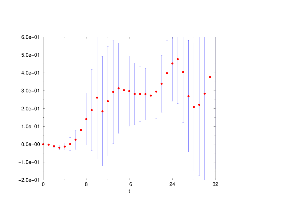
Figure 9: Raw lattice data for the matrix element ${}_{I=0}\langle\pi\pi|O^{-}|K\rangle$ as a function of the time.

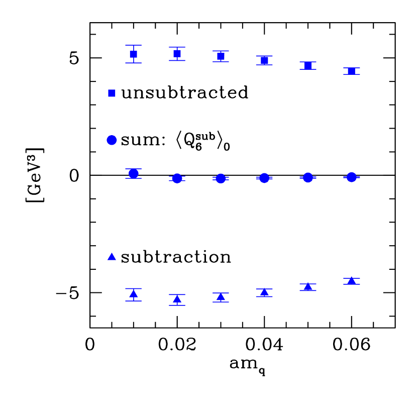
Figure 10: An example of the very large subtractions present in some lattice evaluations of the $\Delta I=1/2$ transitions. The figure shows the values of the unsubtracted and subtracted bare matrix elements ${}_{I=0}\langle\,\pi\pi|O_{6}\,|K\rangle$ as a function of the quark mass from a simulation by the CP-PACS Collaboration [31].

In fig. 10 I illustrate the huge subtractions which generally have to be performed with data from the CP-PACS collaboration for the matrix element of $O_{6}$, which is one of the important operators contributing to $\varepsilon^{\prime}/\varepsilon$.

I now turn to the matrix elements of $\Delta I=3/2$ operators between the kaon and two-pion states. These can can now be evaluated with good precision, and as an example I present in fig. 11 the $\Delta I=3/2$ matrix elements of the electroweak operator $O_{8}$ which is one of the key components in the evaluation of $\varepsilon^{\prime}/\varepsilon$. We are currently undertaking a detailed study, up to next-to-leading order in the chiral expansion for the $\Delta I=3/2$ matrix elements of these operators ($O_{4,7,8}$). Preliminary results indicate that it is possible to obtain a $\Delta I=3/2\,K\to\pi\pi$ decay amplitude, which is nevertheless consistent with a large $B_{K}$ (see sec.2.4).

Figure 11: Preliminary data for the matrix element of the electroweak penguin operator $O_{8}$ for a particular choice of the quark mass as a function of the lattice time $t$ [32].

There is a long history of lattice studies of kaon decays in which operator matrix elements of the type $\langle\pi|O|K\rangle$ are computed and combined with soft-pion theorems and chiral perturbation theory to obtain the decay amplitudes. Here I mention one such recent result, for the matrix element of the electroweak penguin operator $O_{8}$ [19], for which lattice results give significantly smaller values than other determinations, e.g.

$$|_{I=2}\langle\pi\pi|O_{8}|K^{0}\rangle|=(0.5\pm 0.1)\,\textrm{GeV}^{3}\ ,$$ (27)

in the NDR renormalization scheme at a scale of 2 GeV (such a small result was also confirmed from computations of $K\to\pi\pi$ amplitudes by the SPQ${}_{\textrm{CD}}$R collaboration in the presentation of their preliminary data at Lattice 2001 [32]). This can be compared to the larger values, e.g. 2.22$\pm$0.67 GeV³ [33] and (3.5$\pm$1.1) GeV³ [34] obtained using other (continuum) techniques such as dispersion relations and the $1/N_{c}$ expansion . There is also a recent continuum result of 1.2$\pm$0.5 Gev³ [36] obtained using spectral functions. A large value of the matrix element of $O_{8}$ would require very large values indeed for the matrix elements of $O_{6}$ in order to explain the measured value of $\varepsilon^{\prime}/\varepsilon$ and so it will be interesting to follow the developments in these calculations.

As mentioned above, two groups have recently presented results for $\varepsilon^{\prime}/\varepsilon$ and other properties of $K\to\pi\pi$ decay amplitudes, from a computation of $K\to\pi$ matrix elements using the Domain Wall Fermion formulation for lattice quarks (these results were presented since this lecture was delivered). In view of the experimental result [37] $\varepsilon^{\prime}/\varepsilon=(17.2\pm 1.8)\,10^{-4}$ these results may seem somewhat disturbing:

$$\varepsilon^{\prime}/\varepsilon = (-8\div-4)\,10^{-4}\ \ \textrm{RBC}\mbox{\,\cite[cite]{[\@@bibref{}{rbc}{}{}]}}$$ (28)

$$\varepsilon^{\prime}/\varepsilon = (-7\div-2)\,10^{-4}\ \ \textrm{CP-PACS}\mbox{\,\cite[cite]{[\@@bibref{}{cppacs}{}{}]}}.$$ (29)

Of course, it would be very exciting to be able to confidently deduce the existence of new physics from the discrepancy between the lattice results in eqs. (28) and (29) and the experimentally measured value of $\varepsilon^{\prime}/\varepsilon$. Such a conclusion remains a tantalizing possibility. Before this can be done however, we need to be reassured that the systematics of the computations are sufficiently under control. Although the results for $\varepsilon^{\prime}/\varepsilon$ from refs.[38] and [31] are consistent with each other, this is not the case for some other quantities, including some of the separate components in $\varepsilon^{\prime}/\varepsilon$. For example both groups find a large, but different, value for the ratio Re$(A_{0})/$Re$(A_{2})$, where 0 and 2 denote the isospin of the two-pion system (and hence an enhancement of $\Delta I=1/2$ decays !). The RBC collaboration find $\textrm{Re}A_{0}/\textrm{Re}A_{2}=24\div 27$ (remarkably close to the experimental value) whilst CP-PACS find $\textrm{Re}A_{0}/\textrm{Re}A_{2}=9\div 12$. Since both groups use similar methods (but with some important differences, for example in the normalisation of the operators) we need to understand the reason for discrepancies such as these.

It has to be stressed that this calculation is much more difficult and subtle than those reported in section 2. Given the huge subtraction of power divergences, illustrated in fig. 10, a good understanding of the chiral properties of the theory with the parameters used in the simulation is crucial. The computations were performed using Domain Wall Fermions with $N_{5}=16$ points (where $N_{5}$ is the number of points in the fifth direction), and although both groups claim that this is sufficient for the residual chiral symmetry breaking effects to be fully under control, it would be very reassuring to confirm this by increasing $N_{5}$ whilst keeping the other parameters fixed. We also need to be able to understand the consequences for these calculations of the recent observation by Golterman and Pallante [39] that in the quenched approximation there are additional (spurious) chiral logarithms. It should also be remembered that the results for $K\to\pi\pi$ amplitudes in eqs. eqs. (28) and (29) were obtained from the determination of $K\to\pi$ matrix elements using lowest order chiral perturbation theory, and one can ask about the precision of this procedure. Nevertheless, in spite of caveats such as these, these new results are very exciting and mark the beginning of a new era in lattice studies of kaon decays.

4 Conclusion

Lattice simulations provide the opportunity to evaluate non-perturbative QCD effects from first principles with no model assumptions or parameters. There is a large range of quantities of central importance to particle physics which are being computed in lattice simulations (indeed it is far too large a range to be considered in a review talk of 30 minutes). For some quantities, such as those which enter into the analysis of the Unitarity Triangle which were discussed in section 2, the emphasis is now on the reduction of systematic errors. For others, such as the evaluation of nonleptonic weak decays in general and $K\to\pi\pi$ decays in particular, we are still learning how best to extract the physical quantities. The range of quantities which can be studied is constantly expanding.

References

-
[1]
Proceedings of the annual International Symposia on
Lattice Field Theory: Lattice 98 Nucl. Phys. (Proc. Suppl.) 73 (1999); Lattice 99 Nucl. Phys. (Proc. Suppl.) 83
(2000); Lattice 2000 Nucl. Phys. (Proc. Suppl.) 94
(2001); Lattice 2001, copies of transparencies can be found on
http://www-zeuthen.desy.de/
latt2001/ . - [2] Report of the ECFA panel on the future requirements and prospects for Lattice QCD, F. Jegherlehner et al., ECFA-00-200 (2000).
- [3] A. Stocchi, J. Phys. G 27 (2001) 1101.
- [4] S. Hashimoto et al., Phys. Rev. D 61 (2000) 014502.
- [5] UKQCD Collaboration, K.C. Bowler et al., Phys. Rev. D 57 (1998) 6948.
- [6] C. Bernard, Nucl. Phys. Proc. Suppl. 94 (2001) 159.
- [7] UKQCD Collaboration, J. Flynn private communication and J. Gill, hep-lat/0109035.
- [8] CLEO Collaboration, B.H. Behrens et al., Phys. Rev. D 61 (2000) 052001.
- [9] E. El-Khadra et al., Phys. Rev. D 58 (1998) 014506; C.R. Allton et al., Phys.Lett. B 405 (1997) 133; S. Aoki et al., Phys. Rev. Lett. 80 (1998) 5711; C. Bernard et al., Phys. Rev. Lett. 81 (1998) 4812; A. Ali Khan et al., Phys. Lett. B 427 (1998) 132; K-I. Ishikawa et al., Phys. Rev. D 61 (2000) 074501; D. Becirevic et al., Phys.Rev. D 60 (1999) 074501; D. Becirevic et al., hep-lat/0002025; C. Maynard, Nucl. Phys. (Proc.Suppl.) 94 (2001) 367; C.W. Bernard et al., Nucl. Phys. (Proc.Suppl.) 94 (2001) 346; A. Ali Khan et al., Phys.Rev. D 64 (2001) 034505; A. Ali Khan et al., Phys.Rev. D 64 (2001) 054504; L. Lellouch and C.-J. Lin, Phys.Rev. D 64 (2001) 094501.
- [10] S. Collins et al., Phys.Rev. D 60 (1999) 074504; C.W. Bernard et al., Nucl. Phys. (Proc.Suppl.) 94 (2001) 346; A. Ali Khan et al., Phys.Rev. D 64 (2001) 034505; A. Ali Khan et al., Phys.Rev. D 64 (2001) 054504.
-
[11]
Alpha Collaboration,
R. Frezzotti,
P.A. Grassi, S. Sint and P. Weisz, Nucl. Phys. (Proc.Suppl.) 83 (2000) 941; JHEP 0108 (2001) 058. - [12] D. Becirevic, D. Meloni and A. Retico, JHEP 0101 (2001) 012.
- [13] CP-PACS collaboration, A. Ali Khan et al., hep-lat/0105020.
- [14] T. Blum, Nucl. Phys. (Proc.Suppl.) 94 (2001) 291;
- [15] T. Blum and A. Soni, Phys. Rev. Lett. 79 (1997) 3595; T. Blum, Nucl. Phys. (Proc.Suppl.) 94 (2001) 291; A. Ali Khan et al., Nucl. Phys. (Proc.Suppl.) 94 (2001) 287; G. Kilcup, R. Gupta and S.R. Sharpe, Phys. Rev. D 57 (1998) 1654; S. Aoki et al., Phys. Rev. Lett. 80 (1998) 5271; G. Kilcup, D. Pekurovsky and L. Venkataraman Nucl. Phys. (Proc. Suppl.) 53 (1997) 345; 7) S. Aoki et al., Phys. Rev. D 60 (1999) 034511.
- [16] L. Lellouch, Nucl. Phys. Proc. Suppl. 94 (2001) 142.
- [17] S. Sharpe, hep-lat/9811006.
- [18] C.R. Allton et al., Phys. Lett. B 453 (1999) 30.
- [19] A. Donini, V.Giménez, L. Giusti and G. Martinelli, Phys. Lett. B 470 (1999) 233.
- [20] See the talks by D.Cassel, J. Dorfan, J. Nash, M. Neubert, S. Olsen, H. Tajima and M. Wise in these proceedings.
- [21] G. Martinelli, hep-ph/0110023
- [22] C.W. Bernard et al., Phys. Rev. D 32 (1985) 2343; M. Bochiccio et al., Nucl. Phys. B 262 (1985) 331; L. Maiani, G. Martinelli, G.C. Rossi and M. Testa, Phys. Lett. B 176 (1986) 445 and Nucl. Phys. B 289 (1987) 505; C.W. Bernard, T. Draper, G. Hockney and A. Soni, Nucl. Phys. (Proc. Suppl.) 4 (1988) 483; C.Dawson et al., Nucl. Phys. B 514 (1998) 313.
- [23] G. Martinelli et al., Nucl. Phys B 445 (1995) 81; A. Donini et al., Phys. Lett. B 360 (1996) 83; L.Conti et al., Phys. Lett. B 421 (1998) 273.
- [24] C. Dawson et al., Nucl. Phys. (Proc. Suppl.) 94 (2001) 613.
- [25] M. Lüscher, hep-let/9802029 and references therein.
- [26] S. Aoki, T. Izubuchi, Y. Kuramashi, Y. Taniguchi, Phys. Rev. D 59 (1999) 094505 and Phys. Rev. D 60 (1999) 114504; S. Aoki and Y. Kuramashi, Phys. Rev. D 63 (2001) 054504; S. Capitani and L. Giusti, hep-lat/0011070.
- [27] L. Maiani and M. Testa, Phys. Lett. B 245 (1990) 585.
- [28] L. Lellouch and M. Lüscher, Comm. Math. Phys. 219 (2001) 31.
- [29] M. Lüscher, Comm. Math. Phys. 104 (1986) 177; Comm. Math. Phys. 105 (1986) 153; Nucl. Phys. B 354 (1991) 531; Nucl. Phys. B 364 (1991) 237.
- [30] C.-J.D. Lin, G. Martinelli, C.T. Sachrajda and M. Testa, hep-lat/0104006.
- [31] CP-PACS Collaboration, J. Noaki et al., hep-lat/0108013.
- [32] SPQR Collaboration, talks by C.-J.D. Lin, G.Martinelli and M. Papinutto at Lattice 2001.
- [33] J.F. Donoghue and E. Golowich, Phys. Lett. B 478 (2000) 172; V. Cirigliano, J.F. Donohue, E. Golowich and K. Maltman, hep-ph/0109113.
- [34] M. Knecht, S. Peris and E. de.Rafael, Phys. Lett. B 457 (1999) 227; Phys. Lett. B 508 (2001) 117.
- [35] S. Peris and E. de.Rafael, private communication.
- [36] J. Bijnens, E. Gamiz and J. Prades, hep-ph/0108240.
- [37] See the talks by R. Kessler and L. Iconomidou-Fayard in these proceedings.
- [38] RBC Collaboration, Presentations by T. Blum, C. Calin and R. Mawhinney at the 2001 International Symposium on Lattice Field Theory, Berlin, August 19-21 2001.
- [39] M. Golterman and E. Pallante, hep-lat/0108010.