Bremsstrahlung Radiation as Coherent State
in Thermal QED

Abstract

Based on fully finite temperature field theory we investigate the radiation probability in the bremsstrahlung process in thermal QED. It turns out that the infrared divergences resulting from the emission and absorption of the real photons are canceled by the virtual photon exchange processes at finite temperature. The full quantum calculation results for soft photons radiation coincide completely with that obtained in the semi-classical approximation. In the framework of Thermofield Dynamics it is shown that the bremsstrahlung radiation in thermal QED is a coherent state, the quasiclassical behavior of the coherent state leads to above coincidence.

I Introduction

An important aspect of the research on the quark gluon plasma (QGP) is the evidence for its formation in ultrarelativistic heavy ion collision. A lot of fruitful theoretical investigations have been made on the signals for the existence of the QGP, for example, $J/\Psi$ suppression [1], strangeness enhancement[2], jet quenching[3], dilepton and thermal photon production[4] etc. As the electromagnetic signal of the QGP the production of the thermal photon has been investigated by calculating the Compton scattering and $q{\bar{q}}$-annihilation processes in the QGP state[5, 6, 7, 8, 9]. Recent research[10] shows a very interesting result: the bremsstrahlung processes in the QGP state play an important role in the thermal photon production, it generates contribution of the same order of magnitude as Compton scattering and $q{\bar{q}}$-annihilation processes based on the resummation of hard thermal loops[11]. So that the investigation of the bremsstrahlung processes will be a subject of intense theoretical interest. The investigation in Ref. [10] focus on the bresstralung processes with one photon radiation induced by the parton-parton interaction inside QGP. In this paper We consider an external charged particle prepared at remote past goes through the plasma in thermal QED, which produces bresstralung radiation with $N(\geq 1)$ photon radiation by colliding with charged constituent inside the plasma. Such study will be of help to calculate the energy loss of fermion when it goes through the plasma[12].

In the semi-classical approximation (classical charged current coupled with a quantized electromagnetic field) Weldon investigated the bremsstrahlung processes in QED and emphasized on the cancellation of the infrared divergence[13]. In this paper, however, we use fully finite temperature quantum field theoretical method to analyze above bremsstrahlung processes by calculating Feynman diagrams. we will show that the same cancellation of the infrared divergence as in Ref.  [13] occurs in the quantum field theoretical calculation. An interesting result is that quantum calculation results coincide completely with the result obtained in the semi-classical approximation for the radiation probability. We will argue the reason why the quantum effects of the bremstrahlung can be ignored by analyzing the connection between the electromagnetic field in the bremsstrahlung process and coherent state at finite temperature.

This paper is organized as follows: In Sec. II we derive the radiation probability of the bremsstrahlung process by calculating the Feynman diagram in the finite temperature field theory and investigate the cancellation of the infrared divergence. In Sec. III we demonstrate that at finite temperature the radiation of soft photons in the bremsstrahlung processes is a coherent state in the framework of Thermofield Dynamics. A short summary is given in Sec. IV.

II Radiation probability and infrared divergence cancellation

Consider an electron that passes through a plasma in equilibrium state with temperature $T$. The electron accelerates by colliding with the charged constituent inside the plasma and produces the bremsstrahlung radiation.

Now we consider the outgoing electron line in which the electron radiates $n$ photons with momentum $k_{1},k_{2},\cdots,k_{n}$, respectively. Denote the initial four-momentum of the electron as $p$ and the final four-momentum as $p^{\prime}$.For the moment we don’t care whether these are external real photons or virtual photons which connect to each other or the vertices on the incoming electron line. In the calculation we should sum over all possible Feynman diagrams which correspond to $n!$ permutations for the ordering of the momenta $k_{1},k_{2},\cdots,k_{n}$ as illustrated in Fig. 1. If we denote such permutation as $\pi=(\pi(1),\pi(2),\cdots,\pi(n))$ and $\pi(i)$ is the number among $1$ and $n$, then the Dirac structure (the part related to $\gamma$ matrices in the invariant scattering amplitude) of the Feynman diagrams is

$$\sum\limits_{\{\pi\}} \bar{u}(p^{\prime})(-ie\gamma^{\mu_{1}})\frac{i({\not p}^{\prime}+{\not k}_{\pi(1)}+m)}{(p^{\prime}+k_{\pi(1)})^{2}-m^{2}}(-ie\gamma^{\mu_{2}})$$ (3)

$$\frac{i({\not p}^{\prime}+{\not k}_{\pi(1)}+{\not k}_{\pi(2)}+m)}{(p^{\prime}+k_{\pi(1)}+k_{\pi(2)})^{2}-m^{2}}\cdots(-ie\gamma^{\mu_{n}})$$

$$\frac{i({\not p}^{\prime}+{\not k}_{\pi(1)}+\cdots+{\not k}_{\pi(n)}+m)}{(p^{\prime}+k_{\pi(1)}+\cdots+k_{\pi(n)})^{2}-m^{2}}(i{\cal M}_{hard})\,,$$

where $\{\pi\}$ denotes all possible permutation $\pi$. In the following we consider only soft photons radiation. ${\cal M}_{hard}$ denotes the invariant scattering amplitude of hard processes in which no infrared divergence appears. For soft photon emission, $k_{i}$ is small, we will drop the ${\not k}_{i}$ terms in the numerators and the ${\cal O}(k^{2})$ terms in the denominators. It is shown[14] the Dirac structure (3) become

$$\frac{ep^{\prime\mu_{1}}}{p^{\prime}\cdot k_{1}}\frac{ep^{\prime\mu_{2}}}{p^{\prime}\cdot k_{2}}\cdots\frac{ep^{\prime\mu_{n}}}{p^{\prime}\cdot k_{n}}\bar{u}(p^{\prime})(i{\cal M}_{hard})\,.$$ (4)

Similar to the above derivation, for $n$ photons attache to the incoming electron line as illustrated in Fig. 2, the Dirac structure of Feynman diagrams in Fig. 2 is deduced as

$$i{\cal M}_{hard}u(p)\frac{ep^{\mu_{1}}}{-p\cdot k_{1}}\frac{ep^{\mu_{2}}}{-p\cdot k_{2}}\cdots\frac{ep^{\mu_{n}}}{-p\cdot k_{n}}\,.$$ (5)

In general case, for $n$ soft photons emission if we don’t distinguish which one comes from the outgoing or incoming electron line, the Dirac structure corresponding to the sum over all possible Feynman diagrams can be expressed as

$$\bar{u}(p^{\prime}) i{\cal M}_{hard}u(p)\cdot e(\frac{p^{\prime\mu_{1}}}{p^{\prime}\cdot k_{1}}-\frac{p^{\mu_{1}}}{p\cdot k_{1}})$$ (7)

$$e(\frac{p^{\prime\mu_{2}}}{p^{\prime}\cdot k_{2}}-\frac{p^{\mu_{2}}}{p\cdot k_{2}})\cdots e(\frac{p^{\prime\mu_{n}}}{p^{\prime}\cdot k_{n}}-\frac{p^{\mu_{n}}}{p\cdot k_{n}})\,.$$

When calculating the radiation probability of the real photon emission in the thermal equilibrium environment of the plasma, the Boson enhancement factor $1+N(|{\bf k}|)$ should be taken into account in the phase space integration. Here $N(|{\bf k}|)=1/[\exp(|{\bf k}|)-1]$ is the Bose-Einstein distribution function. For the emission of a photon with energy $\omega=|{\bf k}|$, from Eq. (7) we get the radiation probability

$$\frac{dP_{1}}{d\omega} = \int\frac{d\Omega|{\bf k}|^{2}}{(2\pi)^{3}}\frac{e^{2}}{2|{\bf k}|}[1+N(|{\bf k}|)]$$ (9)

$$\cdot\sum\limits_{\lambda}(\frac{p^{\prime\mu}}{p^{\prime}\cdot k}-\frac{p^{\mu}}{p\cdot k})(\frac{p^{\prime\nu}}{p^{\prime}\cdot k}-\frac{p^{\nu}}{p\cdot k})\epsilon_{\mu}^{*}(\lambda)\epsilon_{\nu}(\lambda)$$

$$= \frac{1}{\omega}[1+N(\omega)]A(p^{\prime},p)\,,$$ (10)

where $\epsilon_{\mu}(\lambda)$ is the polarization vector of the photon and function $A(p^{\prime},p)$ has been introduced in Ref. [13],

$$A(p^{\prime},p) = -\frac{e^{2}}{2}\int\frac{d\Omega}{(2\pi)^{3}}(\frac{p^{\prime}}{p^{\prime}\cdot\hat{k}}-\frac{p}{p\cdot\hat{k}})\cdot(\frac{p^{\prime}}{p^{\prime}\cdot\hat{k}}-\frac{p}{p\cdot\hat{k}})$$ (11)

$$= \frac{\alpha}{\pi}[\frac{1}{\upsilon}\ln(\frac{1+\upsilon}{1-\upsilon})-2]\,,$$ (12)

where $\hat{k}=(1,{\bf k}/|{\bf k}|)$ and $v$ is the relative velocity of the final electron in the rest frame of the initial electron defined by $p\cdot p^{\prime}=m^{2}/\sqrt{1-v^{2}}$.

¿From Eq. (9) we see clearly that the radiation probability of a photon can be divided into two parts, the first part is the same as obtained in quantum field theory and it is logarithmic infrared divergent[14]. The second part is the contribution of the thermal effects. As $\omega\rightarrow 0$, $N(\omega)\sim T/\omega$, then the second part

$$\frac{N(\omega)}{\omega}A(p^{\prime},p)\sim\frac{T}{\omega^{2}}A(p^{\prime},p)\,,$$ (13)

which indicates a new infrared divergence emerged in finite temperature field theory and this infrared divergence is linear.

It is different to the quantum field theory at zero temperature, at finite temperature the electron can absorb thermal photon from the heat bath. In getting the absorption probability, the phase space integration should be multiplied by a Boson absorption factor $N(|{\bf k}|)$. It is similar to the above derivation, the probability for absorbing a photon with energy $\omega=|{\bf k}|$ can be deduced as

$$\frac{dP^{\prime}_{1}}{d\omega}=\frac{1}{\omega}N(\omega)A(p^{\prime},p)\,.$$ (14)

We see again the linear infrared divergence resulting from the thermal effects as $\omega\rightarrow 0$.

As well known, in the QED theory at zero temperature the infrared divergences to all order are canceled by taking into account all possible virtual processes[15, 16, 17]. In the following we investigate whether the new infrared divergences emerged in finite temperature field theory can be canceled by the virtual processes.

By picking two photon momenta $k_{i}$ and $k_{j}$ and setting $k_{i}=-k_{j}\equiv k$, we can make a virtual photon. At finite temperature the convenient way for calculating the contribution of virtual photon to the invariant scattering amplitude is to use the real time formalism[18], for single virtual photon exchange process we have

$$X={1\over 2}\int\frac{d^{4}k}{(2\pi)^{4}}{e^{2}}(\frac{p^{\prime\mu_{i}}}{p^{\prime}\cdot k}-\frac{p^{\mu_{i}}}{p\cdot k})(\frac{p^{\prime\mu_{j}}}{-p^{\prime}\cdot k}-\frac{p^{\mu_{j}}}{-p\cdot k})\Delta^{11}_{\mu_{i}\mu_{j}}(k)\,,$$ (15)

where $1/2$ is needed because our procedure counted each Feynman diagram twice, $\Delta^{11}_{\mu_{i}\mu_{j}}(k)$ is the (11)-component of the photon matrix propagator in the real time formalism,

$$\Delta^{11}_{\mu_{i}\mu_{j}}(k)=-g_{\mu_{i}\mu_{j}}\left({i\over{k^{2}+i\eta}}+2\pi N(|k_{0}|)\delta(k^{2})\right)\,.$$ (16)

The real part of $X$ arises from $(1+2N(|k_{0}|))\pi\delta(k^{2})$ term, so that we get

$$\Re(X) = {e^{2}\over 2}\int\frac{d^{4}k}{(2\pi)^{4}}(\frac{p^{\prime}}{p^{\prime}\cdot k}-\frac{p}{p\cdot k})\cdot(\frac{p^{\prime}}{p^{\prime}\cdot k}-\frac{p}{p\cdot k})(1+2N(|k_{0}|))\pi\delta(k^{2})$$ (17)

$$= -\frac{1}{2}A(p^{\prime},p)\int\limits\frac{d|{\bf k}|}{|{\bf k}|}\bigl{(}1+2N(|{\bf k}|)\bigr{)}\,.$$ (18)

Similar to Eq. (9), $\Re(X)$ can be divided into two parts, one part is the same as obtained in quantum field theory and another part is the contribution of the thermal effects. Both parts are all infrared divergent and give negative contribution comparing to the real emission (9) and absorption (14).

The effect of adding one virtual infrared-photon correction to a diagram which does not involve any virtual processes is to multiply the amplitude by a factor $(1+X)$, and thus multiplies the rate by $|1+X|^{2}\approx 1+2\Re(X)$. For $n$ virtual photon exchange processes, each virtual photon will contribute a $X$ to the invariant scattering amplitude, sum over $n$, then the total contribution of all possible virtual photons to the radiation probability can be exponentiated as

$$\left|\sum\limits_{n=0}^{\infty}\frac{X^{n}}{n!}\right|^{2}=e^{2\Re(X)}\,,$$ (19)

where $1/n!$ is a symmetry factor because interchanging virtual photon with each other does not change the diagram.

In the practical calculation of the bremsstrahlung process, all possible emissions and absorptions of the real photons and all possible exchanges of the virtual photon should be taken into account at the same time. So that the probability of radiating a net energy $E$ is

$$\frac{dP}{dE} = \exp[2\Re(X)]\sum\limits_{n=1}^{\infty}\int\frac{1}{n!}d\Phi_{1}d\Phi_{2}\cdots d\Phi_{n}$$ (22)

$$\delta(k^{0}_{1}+k^{0}_{2}+\cdots+k^{0}_{n}-E){\prod\limits_{i=1}^{n}}\sum\limits_{\lambda}e^{2}(\frac{p^{\prime\mu}}{p^{\prime}\cdot k_{i}}-\frac{p^{\mu}}{p\cdot k_{i}})$$

$$(\frac{p^{\prime\nu}}{p^{\prime}\cdot k_{i}}-\frac{p^{\nu}}{p\cdot k_{i}})\epsilon_{\mu}^{*}(\lambda)\epsilon_{\nu}(\lambda)\,,$$

where $1/n!$ is symmetry factor because $n$ photons are identical particles, and $d\Phi_{i}$ is integration of phase space. For emission ($k^{0}_{i}=|{\bf k}_{i}|$) and absorption ($k^{0}_{i}=-|{\bf k}_{i}|$), $d\Phi_{i}$ is defined as

$$d\Phi_{i} = \frac{d^{3}|{\bf k}_{i}|}{(2\pi)^{3}}\frac{1}{2|{\bf k}_{i}|}\times\cases{1+N(|{\bf k}_{i}|),&if $k^{0}_{i}=|{\bf k}_{i}|$\cr N(|{\bf k}_{i}|),&if $k^{0}_{i}=-|{\bf k}_{i}|$\cr}$$ (23)

$$= \frac{d^{4}k_{i}}{(2\pi)^{3}}\delta(k_{i}^{2})[\theta(k_{i}^{0})+N(|{\bf k}_{i}|)]\,.$$ (24)

¿From Eq. (22) it is easy to deduce

$$\frac{dP}{dE}=\int\limits_{-\infty}^{+\infty}\frac{dt}{2\pi}e^{-iEt}e^{\bar{R}(t)}\,,$$ (25)

where

$$\bar{R}(t) = 2\Re(X)+R(t)\,,$$ (26)

$$R(t) = -e^{2}\int d\Phi_{i}e^{ik^{0}_{i}t}(\frac{p^{\prime}}{p^{\prime}\cdot k_{i}}-\frac{p}{p\cdot k_{i}})$$ (28)

$$\qquad\cdot(\frac{p^{\prime}}{p^{\prime}\cdot k_{i}}-\frac{p}{p\cdot k_{i}})\,.$$

Both $\Re(X)$ and $R(t)$ contain infrared divergence, but the sign is opposite. Inserting Eqs. (17) and (28) into Eq.(26) we get

$${\bar{R}(t)} = A(p^{\prime},p)\int\frac{d|{\bf k}|}{|{\bf k}|}\Bigl{[}\bigl{(}1+N(|{\bf k}|)\bigr{)}e^{i|{\bf k}|t}$$ (30)

$$\qquad+N(|{\bf k}|)e^{-i|{\bf k}|t}-\bigl{(}1+2N(|{\bf k}|)\bigr{)}\Bigr{]}\,.$$

If $|{\bf k}|$ is small, then $N(|{\bf k}|)\sim T/|{\bf k}|$ and $e^{i|{\bf k}|t}\sim 1+i|{\bf k}|t$. Substitute them into Eq. (30), the linear and the logarithmic divergent terms are canceled exactly, so that the radiation probability (25) is finite in the infrared region at finite temperature.

In order to perform the integration in Eq. (30) it is convenient to introduce a cutoff factor $\exp(-|{\bf k}|/\Lambda)$ to the integrand in the ultraviolet region. After introducing this cutoff factor, the radiation probability (25) coincides completely with the result,

$$\frac{dP}{dE}=\left|\Gamma\left(\frac{A}{2}+i\frac{E}{2\pi T}\right)\right|^{2}\frac{e^{E/2T}e^{-|E|/\Lambda}}{4\pi^{2}T\Gamma(A)}\left(\frac{2\pi T}{\Lambda}\right)^{A}\,,$$ (31)

which has been obtained in Ref. [13] in the semi-classical approximation.

III Connection between bremsstrahlung radiation and coherent state

In above full quantum field theoretical calculation we consider only soft photons. The full quantum calculation result is completely the same as that obtained in the semi-classical approximation. It seems that the quantum effects is unimportant for soft photon radiation in bremsstrahlung process. In the following we argue the reason.

Now we calculate the probability of producing $n$ photons in bremsstrahlung process. Suppose the energy of all photons is between $\omega$ and $\omega+\Delta\omega$. The contribution of all virtual photons to probability amplitude is

$$\Re(X^{\prime})=-\frac{1}{2}A(p^{\prime},p)\int\limits_{\omega}^{\omega+\rm\Delta\omega}\frac{d|{\bf k}|}{|{\bf k}|}\bigl{(}1+2N(|{\bf k}|)\bigr{)}\,.$$ (32)

The probability for producing $n$ photon with energy between $\omega$ and $\omega+\Delta\omega$ can be expressed as

$$P_{n}(\omega) = \exp[2\Re(X^{\prime})]\frac{1}{n!}{\prod\limits_{i=1}^{n}}\sum_{\lambda}\int\limits_{\omega}^{\omega+\rm\Delta\omega}d\Phi_{i}$$ (34)

$$e^{2}(\frac{p^{\prime\mu}}{p^{\prime}\cdot k_{i}}-\frac{p^{\mu}}{p\cdot k_{i}})(\frac{p^{\prime\nu}}{p^{\prime}\cdot k_{i}}-\frac{p^{\nu}}{p\cdot k_{i}})\epsilon_{\mu}^{*}(\lambda)\epsilon_{\nu}(\lambda)$$

$$= {{\lambda^{n}}\over n!}e^{-\lambda}\,.$$ (35)

It is a Poisson distribution. The average photon number is

$$\langle n\rangle=\lambda=A(p^{\prime},p)\int\limits_{\omega}^{\omega+\rm\Delta\omega}\frac{d|{\bf k}|}{|{\bf k}|}[1+2N(|{\bf k}|)]\,.$$ (36)

At high temperature limit $T\gg 1$, $N(|{\bf k}|)\sim T/|{\bf k}|$, we see that the average photon number increases linearly with increasing temperature.

It is known that at zero temperature the final state in the bremsstrahlung process is a coherent state and the distribution of the photon are also a Poisson distribution[19] like Eq.(34). This stimulate us to investigate whether the bremsstrahlung radiation result from a coherent state at finite temperature.

In the following we demonstrate that at finite temperature the photon radiation in the bremsstrahlung process really does come from a coherent state of the field operator in the framework of Thermofield Dynamics[20]. In the Thermofield Dynamics a so-called tilde system which is identical to the original system has been introduced in order to define the thermal vacuum state and the thermal field operator. The complete Lagrangian for the combined system describing the radiation of photons by a classical current $j_{\mu}(x)$ is

$${\hat{\cal L}}={\cal L}-{\tilde{\cal L}}\,,$$ (37)

where the Lagrangian for original and tilde system are

$${\cal L} = -\left({1\over 4}F_{\mu\nu}F^{\mu\nu}+j_{\mu}A^{\mu}\right)\,,$$ (38)

$${\tilde{\cal L}} = -\left({1\over 4}{\tilde{F}}_{\mu\nu}{\tilde{F}}^{\mu\nu}+{\tilde{j}}_{\mu}{\tilde{A}}^{\mu}\right)\,,$$ (39)

respectively. In Thermofield Dynamics we introduce the doublet field and source

$${\cal A}_{\mu}(x)=\left(\begin{array}[]{cc}A_{\mu}(x)\\ {\tilde{A}}_{\mu}(x)\end{array}\right)\,,\qquad{\cal J}_{\mu}(x)=\left(\begin{array}[]{cc}j_{\mu}(x)\\ {\tilde{j}}_{\mu}(x)\end{array}\right)\,.$$ (40)

For the bremsstrahlung process we can assume that the current ${\cal J}_{\mu}(x)$ is switched on adiabatically on a finite time interval. Use the retarded and advanced Green function the solution of the equation of motion for field ${\cal A}_{\mu}(x)$ at zero temperature can be expressed as

$${\cal A}_{\mu}(x) = {\cal A}_{\mu}^{in}(x)+\int d^{4}yG_{\mu\nu}^{ret}(x-y){\cal J}^{\nu}(y)$$ (41)

$$= {\cal A}_{\mu}^{out}(x)+\int d^{4}yG_{\mu\nu}^{adv}(x-y){\cal J}^{\nu}(y)\,.$$ (42)

The quantum free field ${\cal A}_{\mu}^{in}(x)$ and ${\cal A}_{\mu}^{out}(x)$ describe the photon field before and after its interaction with the current ${\cal J}_{\mu}$, then we have

$${\cal A}_{\mu}^{in}(x)=\lim_{x_{0}\rightarrow-\infty}{\cal A}_{\mu}(x)\,,\qquad{\cal A}_{\mu}^{out}(x)=\lim_{x_{0}\rightarrow+\infty}{\cal A}_{\mu}(x)\,.$$ (43)

At zero temperature the retarded and advanced Green function can be written as

$$iG_{\mu\nu}^{ret}(x-y) = \theta(t_{x}-t_{y})\langle 0,{\tilde{0}}|\left(\begin{array}[]{cc}[A_{\mu}^{(0)}(x),A_{\nu}^{(0)}(y)],&0\\ 0,&[{\tilde{A}}_{\mu}^{(0)}(x),{\tilde{A}}_{\nu}^{(0)}(y)]\end{array}\right)|0,{\tilde{0}}\rangle\,,$$ (46)

$$iG_{\mu\nu}^{adv}(x-y) = -\theta(t_{y}-t_{x})\langle 0,{\tilde{0}}|\left(\begin{array}[]{cc}[A_{\mu}^{(0)}(x),A_{\nu}^{(0)}(y)],&0\\ 0,&[{\tilde{A}}_{\mu}^{(0)}(x),{\tilde{A}}_{\nu}^{(0)}(y)]\end{array}\right)|0,{\tilde{0}}\rangle\,.$$ (49)

In the Thermofield Dynamics the connection between usual vacuum $|0,{\tilde{0}}\rangle$ and the thermal vacuum $|0,\beta\rangle$ is a Bogoliubov transformation[20],

$$|0,\beta\rangle = U(\theta)|0,{\tilde{0}}\rangle\,,$$ (50)

$$U(\theta) = \exp\left[-\sum_{\bf k}\theta_{\bf k}(\beta)\left({\tilde{a}}_{\bf k}a_{\bf k}-a^{{\dagger}}_{\bf k}{\tilde{a}}_{\bf k}^{{\dagger}}\right)\right]\,,$$ (51)

with

$$\cosh\theta_{\bf k}(\beta)={1\over\sqrt{1-e^{-\beta|{\bf k}|}}}\,,\qquad\sinh\theta_{\bf k}(\beta)={e^{\beta|{\bf k}/2}\over\sqrt{1-e^{-\beta|{\bf k}|}}}\,,$$ (52)

where $\beta=1/T$. From Eq.(41) corresponding thermal field can be expressed as

$${\cal A}_{\mu}(x,\beta) = U^{{\dagger}}(\theta){\cal A}_{\mu}(x)U(\theta)$$ (53)

$$= {\cal A}_{\mu}^{in}(x,\beta)+\int d^{4}yG_{\mu\nu}^{ret}(x-y,\beta){\cal J}^{\nu}(y,\beta)$$ (54)

$$= {\cal A}_{\mu}^{out}(x,\beta)+\int d^{4}yG_{\mu\nu}^{adv}(x-y,\beta){\cal J}^{\nu}(y,\beta)\,,$$ (55)

where corresponding thermal field, retarded and advanced Green function and the source are

$${\cal A}_{\mu}^{in,out}(x,\beta) = U^{{\dagger}}(\theta){\cal A}_{\mu}^{in,out}(x)U(\theta)\,,$$ (56)

$$G_{\mu\nu}^{ret,adv}(x-y,\beta) = U^{{\dagger}}(\theta)G_{\mu\nu}^{ret,adv}(x-y)U(\theta)\,,$$ (57)

$${\cal J}_{\mu}(x,\beta) = U^{{\dagger}}(\theta){\cal J}_{\mu}(x)U(\theta)\,.$$ (58)

¿From Eq.(53) we obtain

$${\cal A}_{\mu}^{out}(x,\beta) = {\cal A}_{\mu}^{in}(x,\beta)+\int d^{4}y\left[G_{\mu\nu}^{ret}(x-y,\beta)-G_{\mu\nu}^{adv}(x-y,\beta)\right]{\cal J}^{\nu}(y,\beta)$$ (59)

$$= {\cal A}_{\mu}^{in}(x,\beta)+{\cal A}_{\mu}^{cl}(x,\beta)\,,$$ (60)

where ${\cal A}_{\mu}^{cl}(x,\beta)$ is the classical thermal field radiated by the current ${\cal J}(x,\beta)$ at finite temperature.

Define the thermal in- and out-state connecting the thermal in- and out-state field as $|0,\beta\rangle_{in}$ and $|0,\beta\rangle_{out}$, respectively. They are connected by a unitary operator $S$ as

$$|0,\beta\rangle_{out}=S|0,\beta\rangle_{in}\,.$$ (61)

Then we have

$${\cal A}_{\mu}^{out}(x,\beta)=S^{-1}{\cal A}_{\mu}^{in}(x,\beta)S\,.$$ (62)

The thermal vacuum state $|0,\beta\rangle_{in}$ is an eigenvector of the annihilation part ${\cal A}_{\mu}^{in(+)}(x,\beta)$ with positive frequency,

$${\cal A}_{\mu}^{in(+)}(x,\beta)|0,\beta\rangle_{in}=0\,.$$ (63)

¿From Eq.(59) we have

$${\cal A}_{\mu}^{out(+)}(x,\beta)|0,\beta\rangle_{in} = S^{-1}{\cal A}_{\mu}^{in(+)}(x,\beta)S|0,\beta\rangle_{in}$$ (64)

$$= {\cal A}_{\mu}^{cl(+)}(x,\beta)|0,\beta\rangle_{in}\,.$$ (65)

This expression lead to

$${\cal A}_{\mu}^{in(+)}(x,\beta)|0,\beta\rangle_{out}={\cal A}_{\mu}^{cl(+)}(x,\beta)|0,\beta\rangle_{out}\,.$$ (66)

Eq.(66) indicate that at finite temperature the final state in bremsstrahlung process is a coherent state because it is just the eigenstate of annihilation thermal field operator.

The main features of the coherent state are that the coherent state is represented by a minimum uncertainty wave packet, the quantum correlation in these states is absent, so that the coherent state behaves as a quasiclassical state. It is the quasiclassical property of the coherent state which leads to that our full quantum calculation results coincides completely with that obtained in the semi-classical approximation.

IV Conclusion

By directly calculating the Feynman diagram, we use fully finite temperature field theoretical method to derive the radiation probability of the bremsstrahlung processes in thermal QED. It is shown that the infrared divergence are canceled to each other by taking into account the real photon emission, absorption and virtual photon exchange processes at the same time. The radiation probability for soft photons coincides completely with the result obtained in the semi-classical approximation. At zero temperature it is known that the bremsstrahlung radiation comes from the coherent state, we generalize this argument to the finite temperature case. Based on the Thermofield Dynamics it is shown that the final state in bremsstrahlung process is a coherent state at finite temperature. Because the coherent state is a state which is the most approachable to classical limit and is permitted to exist in quantum theory, this quasiclassical features makes that the semi-classical approximation produces same result as the quantum calculation.

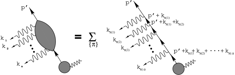
FIG. 1.: Feynman diagram for the outgoing electron line radiating $n$ photons.

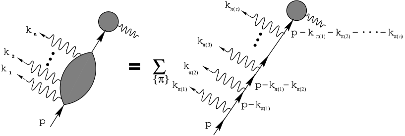
FIG. 2.: Same as Fig. 1 but for incoming electron line.

- [1] T. Matsui and H. Satz, Phys. Lett. B178 (1986) 416.
- [2] J. Rafelski and B. Müller, Phys. Rev. Lett. 48 (1982) 1066.
- [3] X.-N. Wang and M. Gyulassy, Phys. Rev. Lett. 68 (1992) 1480; M. Gyulassy, M. Plümer, M. H. Thoma and X.-N. Wang, Nucl. Phys. A538 (1992) 37c.
- [4] P.V. Ruuskanen, Nucl. Phys. A544 (1992) 169c.
- [5] J. Kapusta, P. Lichard and D. Seibert, Phys. Rev. D44 (1991) 2774.
- [6] R. Baier, H. Nakkagawa, A. Niegawa and K. Redlich, Z. Phys. C53 (1992) 433.
- [7] N. Arbex, U. Ornik, M. Plümer, A. Timmermann and R. M. Weiner, Phys. Lett. B345 (1995) 307.
- [8] J. Sollfrank, P. Huovinen, M. Kataja, P. V. Ruskanen, M. Prakash and R. Venugopalan, Phys. Rev. C55 (1997) 392.
- [9] J. Cleymans, K. Redlich and D. K. Srivastava, Phys. Rev. C55 (1997) 1431.
- [10] P. Aurenche, F. Gelis, R. Kobes and H. Zaraket, Phys. Rev. D58 (1998) 085003; P. Aurenche, F. Gelis, H. Zaraket, hep-ph/0003326.
- [11] R. D. Pisarski, Phys. Rev. Lett. 63 (1989) 1129; E. Braaten, R. D. Pisarski, Nucl. Phys. B337 (1990), 569; Nucl. Phys. B339 (1990), 310.
- [12] X.-N. Wang, Phys. Rep. 280 (1997) 287; E. Wang and X.-N. Wang, Nucl-th/0106043.
- [13] H. A. Weldon, Phys. Rev. D49 (1994) 1579.
- [14] See, for example, M. E. Peskin and D. V. Schroeder, An Introduction to Quantum Field Theory (Addison-Wesley Publishing Company, 1995).
- [15] F. Bloch and A. Nordsieck, Phys. Rev. 52 (1937) 54.
- [16] D. Yennie, S. Frautschi and H. Suura, Ann. Phys. 13 (1961) 379.
- [17] S. Weinberg, Phys. Rev. 140 (1965) B516.
- [18] See, for example, M. Le Bellac, Thermal Field Theory (Cambridge University Press, 1996).
- [19] See, for example, C. Itzykson and J.-B. Zuber Quantum Field Theory (McGraw-Hill Inc. Newyork, 1980).
- [20] Y. Takahashi and H. Umezawa, Collective Phenomena 2 (1975) 55; H. Umezawa, H. Matsumoto and M. Tachiki, Thermofield Dynamics and Condensed Matter (North-Holland, 1982).