The spontaneous generation of magnetic and chromomagnetic fields at high temperature in the Standard Model

Abstract

The spontaneous generation of the magnetic and chromomagnetic fields at high temperature is investigated in the Standard Model. The consistent effective potential including the one-loop and the daisy diagrams of all boson and fermion fields is calculated. The mixing of the generated fields due to the quark loop diagram is studied in detail. It is found that the quark contribution increases the magnetic and chromomagnetic field strengths as compared with the separate generation of fields. The magnetized vacuum state is stable due to the magnetic gauge field masses included in the daisy diagrams. Some applications of the results obtained are discussed.

1 Introduction

One of interesting problems of nowadays high energy phy- sics is generation of strong magnetic fields in the early universe. Different mechanisms of producing the fields at different stages of the universe evolution have been proposed (see, for instance, the surveys Ken ; Ken2 ; Dar ) and the influence of fields on various processes was discussed. In particular, the primordial magnetic fields, being implemented in cosmic plasma, may serve as the seed source of the present extra galaxy fields.

One of the mechanisms is a spontaneous vacuum magnetization at high temperature. It was investigated already for the case of pure $SU(2)$ gluodynamics in Refs. Enq ; Sta ; Once , where it has been shown the possibility of this phenomenon. The stability of the magnetized vacuum was also studied Once . As it is well known, the magnetization takes place for the non-abelian gauge fields due to a vacuum dynamics Sv . In fact, this is one of the distinguishable features of asymptotically free theories. In the papers mentioned the fermions were not taken into consideration. However, they may affect the vacuum state due to loop corrections in strong magnetic fields at high temperature.

In the present paper the spontaneous vacuum magnetization is investigated in the standard model (SM) of elementary particles. All boson and fermion fields are taken into consideration. In the SM there are two kind of non-abelian gauge fields - the $SU(2)$ weak isospin gauge fields responsible for weak interactions and the $SU(3)$ gluons mediating strong interactions. The quarks possess both the electric and colour charges. So, they have to mix the chromomagnetic and the ordinary magnetic fields due to vacuum loops. Because of this mixing some specific configurations of the fields must be produced at high temperature. To elaborate this picture quantitatively, we calculate the effective potential (EP) including the one-loop and the daisy diagram contributions in the constant abelian chromomagnetic and magnetic fields, $H_{c}=const$ and $H=const$, at high temperatures. This type of resummations guarantees a vacuum stability if one takes into consideration the one-loop temperature masses of the transversal gauge fields in the external fields considered Once . So, we will used this approximation in what follows. Since an abelian magnetic hypercharge field is not generated spontaneously, in what follows we shall consider the non-abelian component of the magnetic field. The mechanisms of hypermagnetic field generation has been discussed in Refs. Gio ; Jo . It will be shown that at high temperatures either the strong magnetic or the chromomagnetic fields are generated. They are stable in the approximation adopted due to the magnetic masses of $m^{2}_{transversal}\sim(gH)^{1/2}T$ of the gauge field transversal modes SkSt . In this way the consistent picture of the magnetized vacuum state in the SM at high temperature can be derived.

The paper content is as follows. In sect. 2 the contributions of bosons and fermions to the EP $v^{\prime}(H,T)$ of external magnetic and chromomagnetic fields are calculated in the form convenient for numeric investigations. In sect. 3 the field strengths are calculated. Discussion and concluding remarks are given in sect. 4.

2 Basic Formulae

The SM Lagrangian of the gauge boson sector is (see, for example, Cheng )

$$L=-\frac{1}{4}F^{\alpha}_{\mu\nu}F^{\mu\nu}_{\alpha}-\frac{1}{4}G_{\mu\nu}G^{\mu\nu}-\frac{1}{4}{\bf F}^{\alpha}_{\mu\nu}{\bf F}^{\mu\nu}_{\alpha},$$ (1)

where the standard notations are introduced

$$F^{\alpha}_{\mu\nu}=\partial_{\mu}A^{\alpha}_{\nu}-\partial_{\nu}A^{\alpha}_{\mu}+g\epsilon^{abc}A^{b}_{\mu}A^{c}_{\nu},$$ (2)

$$G_{\mu\nu}=\partial_{\mu}B_{\nu}-\partial_{\nu}B_{\mu},$$

$${\bf F}^{\alpha}_{\mu\nu}=\partial_{\mu}{\bf A}^{\alpha}_{\nu}-\partial_{\nu}{\bf A}^{\alpha}_{\mu}+g_{s}f^{abc}{\bf A}^{b}_{\mu}{\bf A}^{c}_{\nu}.$$

The fields corresponding to the $W-$, $Z-$bosons and photons, respectively, are

$$W_{\mu}^{\pm}=\frac{1}{\sqrt{2}}(A^{1}_{\mu}\pm iA^{2}_{\mu}),$$ (3)

$$Z_{\mu}=\frac{1}{\sqrt{g^{2}+g^{\prime 2}}}(gA^{3}_{\mu}-g^{\prime}B_{\mu}),$$

$$A_{\mu}=\frac{1}{\sqrt{g^{2}+g^{\prime 2}}}(g^{\prime}A^{3}_{\mu}+gB_{\mu})$$

and ${\bf A^{\alpha}_{\mu}}$ is the gluon field.

To introduce an interaction with the magnetic and chromomagnetic fields we replace all derivatives in the Lagrangian by the covariant ones,

$$\partial_{\mu}\to{\cal D}_{\mu}=\partial_{\mu}+ig\frac{\tau^{\alpha}}{2}A^{\alpha}_{\mu}+ig_{s}\frac{\lambda^{\alpha}}{2}{\bf A}_{\mu}^{\alpha}.$$ (4)

Here $\tau^{\alpha}$ and $\lambda^{\alpha}$ stand for the Pauli and the Gell-Mann matrices, respectively.

In the $SU(2)$ sector of the SM there is only one magnetic field - the third projection of the gauge field. In the $SU(3)_{c}$ sector there are two possible chromomagnetic fields connected with the third and eighth generators of the $SU(3)$.

For simplicity, in what follows we shall consider the field associated with the third generator of the $SU(3)_{c}$.

The introduction of an interaction with classical magnetic and chromomagnetic fields as usually is doing by splitting the potentials in two parts

$$A_{\mu}=\bar{A}_{\mu}+A^{R}_{\mu},$$ (5)

$${\bf A}_{\mu}=\bar{\bf A}_{\mu}+{\bf A}^{R}_{\mu},$$

where $A^{R}$ and ${\bf A}^{R}$ describe the radiation fields and $\bar{A}=$ $(0,0,Hx^{1},0)$ and $\bar{\bf A}=(0,0,{\bf H}_{3}x^{1},0)$ correspond to the constant magnetic   and   chromomagnetic fields directed along the third axes in the space and in the internal colour and isospin spaces.

We used the general relativistic renormalizable gauge which is set by the following gauge-fixing conditions VVk

$$\partial_{\mu}W^{\pm\mu}\pm ie\bar{A}_{\mu}W^{\pm\mu}\mp i\frac{g\phi_{c}}{2\xi}\phi^{\pm}=C^{\pm}(x),$$ (6)

$$\partial_{\mu}Z^{\mu}-\frac{i}{\xi^{\prime}}(g^{2}+g^{\prime 2})^{1/2}\phi_{c}\phi_{Z}=C^{Z}(x),$$

$$\partial_{\mu}{\bf A}^{\mu}+ig_{s}\bar{\bf A}={\bf C}(x),$$

where $e=g~{}sin\theta_{W}$, $tan\theta_{W}=g^{\prime}/g$, $\phi^{\pm}$ and $\phi_{Z}$ are the Goldstone fields, $\xi$ and $\xi^{\prime}$ are the gauge fixing parameters, $C^{\pm}$ and $C^{Z}$ are arbitrary functions and $\phi_{c}$ is a value of the scalar field condensate. Setting $\xi,\xi^{\prime}=0$ we choose the unitary gauge. In the restored phase the scalar field condensate $\phi_{c}=0$ and the equations (6) are simplified.

The values of the macroscopic magnetic and chromomagnetic fields generated at high temperature will be calculated by minimization of the thermodynamics potential.

The thermodynamic potential $\Omega$ of the model is

$$\Omega=-\frac{1}{\beta}log~{}Z,$$ (7)

$$Z=Tr~{}exp(-\beta{\cal{H}}),$$ (8)

where $Z$ is the partition function, ${\cal{H}}$ is the Hamiltonian of the system. The trace is calculated over all physical states.

To obtain the EP one has to rewrite (7) as a sum in quantum states calculated near the nontrivial classical solutions $A^{ext}$ and ${\bf A}^{ext}$. This procedure is well-described in literature (see, for instance, Once ; Kap ; Carr ) and the result can be written in the form:

$$V=V^{(1)}(H,{\bf H}_{3},T)+V^{(2)}(H,{\bf H}_{3},T)+...$$ (9)

$$+V_{daisy}(H,{\bf H}_{3},T)+...,$$

where $V^{(1)}$ is the one-loop EP, the other terms present the contributions of two-, three-, etc. loop corrections.

Among these terms there are ones responsible for dominant contributions of long distances at high temperature - so-called daisy or ring diagrams (see, for example, Kap ). This part of the EP, $V_{daisy}(H,{\bf H}_{3},T)$, is nonzero in the case when massless states appear in a system. The ring diagrams have to be calculated when the vacuum magnetization at finite temperature is investigated. Really, one first must assume that the fields are nonzero, calculate EP $V(H,{\bf H}_{3},T)$ and after that check whether its minimum is located at nonzero $H$ and ${\bf H}_{3}$. On the other hand, if one investigates problems in the applied external fields, the charged fields become massive with the masses depending on $\sim(gH)^{1/2}$, $\sim(g_{s}{\bf H}_{3})^{1/2}$ and have to be omitted.

The one-loop contribution into EP is given by the expression

$$V^{(1)}=-\frac{1}{2}Tr~{}log~{}G^{ab},$$ (10)

where $G^{ab}$ stands for the propagators of all quantum fields $W^{\pm}$, ${\bf A}$, $\ldots$ in the background fields $H$ and ${\bf H}_{3}$. In the proper time formalism, $s$-representation, the calculation of the trace can be carried out in accordance with the formula Schw

$$Tr~{}log~{}G^{ab}=-\int_{0}^{\infty}\frac{ds}{s}tr~{}exp(-isG^{-1}_{ab}).$$ (11)

Details of calculations based on the $s$-representation and formula (2) can be found in Refs. Cab , Rez and Ska .

We make use the method of Ref. Cab allowing in a natural way to incorporate the temperature into this formalism. A basic formula of Ref. Cab connecting the Matsubara Green functions with the Green functions at zero temperature is needed,

$$G^{ab}_{k}(x,x^{\prime}; T)=$$

$$\sum^{+\infty}_{-\infty}(-1)^{(n+[x])\sigma_{k}}G^{ab}_{k}(x-[x]\beta u,x^{\prime}-n\beta u),$$

where $G^{ab}_{k}$ is the corresponding function at $T=0$, $\beta=1/T$, $u=(0,0,0,1)$, $[x]$ denotes an integer part of $x_{4}/\beta$, $\sigma_{k}=1$ in the case of physical fermions and $\sigma_{k}=0$ for boson and ghost fields. The Green functions in the right-hand side of (2) are the matrix elements of the operators $G_{k}$ computed in the states $|x^{\prime},a\rangle$ at $T=0$, and in the left-hand side the operators are averaged over the states with $T\neq 0$. The corresponding functional spaces $U^{0}$ and $U^{T}$ are different but in the limit of $T\to 0$ $U^{T}$ transforms into $U^{0}$.

The terms with $n=0$ in Eqs. (2), (10) give the zero temperature expressions for the Green functions and the effective potential $V^{\prime}$, respectively. So, we can split it into two parts:

$$V^{\prime}(H,{\bf H}_{3},T)=V^{\prime}(H,{\bf H}_{3})+V^{\prime}_{\tau}(H,{\bf H}_{3},T).$$ (13)

The standard procedure to account for the daisy diagrams is to substitute the tree level Matsubara Green functions in (10) $[G^{(0)}_{i}]^{-1}$ by the full propagator $G^{-1}_{i}=[G^{(0)}_{i}]^{-1}+\Pi(H,T)$ (see for details Once , Kap , Carr ), where the last term is polarization operator at finite temperature in the field taken at zero longitudinal momentum $k_{l}=0$.

Passing the detailed calculations we can notice that the exact one-loop EP will transformed into EP, which contains the daisy diagrams as well as one-loop diagrams, by adding term contained the temperature dependent mass of particle to the exponent.

It is convenient for what follows to introduce the dimensionless quantities: $x=H/H_{0}$ $(H_{0}=M_{W}^{2}/e)$, $y={\bf H}_{3}/{\bf H}_{3}^{0}$ $({\bf H}_{3}^{0}=M_{W}^{2}/g_{s})$, $B=\beta M_{W}$, $\tau=1/B=T/M_{W}$, $v=V/H_{0}^{2}$.

The total EP in our consideration consists of the several terms

$$v^{\prime} = \frac{x^{2}}{2}+\frac{y^{2}}{2}+v^{\prime}_{leptons}+v^{\prime}_{quarks}$$

$$+v^{\prime}_{W-bosons}+v^{\prime}_{gluons}.$$

These terms can be exactly written for SM fields (in dimensionless variables):

- leptons

$$v^{\prime}_{leptons}=-\frac{1}{4\pi^{2}}\sum_{n=1}^{\infty}(-1)^{n}\int_{0}^{\infty}\frac{ds}{s^{3}}$$ (15)

$$\cdot e^{-(m_{leptons}^{2}s+\frac{\beta^{2}n^{2}}{4s})}(xs~{}Coth(xs)-1);$$

- quarks

$$v^{\prime}_{quarks}=-\frac{1}{4\pi^{2}}\sum_{f=1}^{6}\sum_{n=1}^{\infty}(-1)^{n}\int_{0}^{\infty}\frac{ds}{s^{3}}e^{-(m_{f}^{2}s+\frac{\beta^{2}n^{2}}{4s})}$$ (16)

$$\cdot(q_{f}xs~{}Coth(q_{f}xs)\cdot ys~{}Coth(ys)-1);$$

- $W$-bosons (see EW )

$$v^{\prime}_{W}=-\frac{x}{8\pi^{2}}\sum_{n=1}^{\infty}\int_{0}^{\infty}\frac{ds}{s^{2}}e^{-(m_{W}^{2}s+\frac{\beta^{2}n^{2}}{4s})}$$ (17)

$$\cdot\left[\frac{3}{Sinh(xs)}+4Sinh(xs)\right];$$

- gluons (see Once )

$$v^{\prime}_{gluons}=-\frac{y}{4\pi^{2}}\sum_{n=1}^{\infty}\int_{0}^{\infty}\frac{ds}{s^{2}}e^{-(m_{gluons}^{2}s+\frac{\beta^{2}n^{2}}{4s})}$$ (18)

$$\cdot\left[\frac{1}{Sinh(ys)}+2Sinh(ys)\right].$$

Here, $m_{leptons}$, $m_{f}$, $m_{W}$ and $m_{gluons}$ are the temperature masses of leptons, quarks, W-bosons and gluons, respectively; $q_{f}=\left(\frac{2}{3},-\frac{1}{3},-\frac{1}{3},\frac{2}{3},-\frac{1}{3},\frac{2}{3}\right)$ - the charges of quarks.

Since we investigate the dynamics of high-temperature effects connected with the presence of external fields, we used only the leading in temperature terms of the Debye masses of the particles (Once , EW ).

The temperature masses of leptons and quarks are

$$\begin{array}[]{cc}m_{leptons}^{2}=\left(\frac{e}{\beta}\right)^{2},&m_{f}^{2}=\left(\frac{e}{\beta}\right)^{2}.\end{array}$$ (20)

As it is known Once , the transversal components of the charged gluons and $W$-bosons have no temperature masses of order $\sim g_{s}{\bf H}_{3}$ and $\sim gH$. Only the longitudinal components have the Debye masses, but they are $H$- and ${\bf H}_{3}$-independent, therefore, they can be omitted in our consideration. Instead, the transversal component masses, which depend on the Landau level number, must be used. So, the transversal temperature masses of $W-$bosons and charged gluons

$$\begin{array}[]{cc}m_{W}^{2}=15\alpha_{e.w.}\frac{h^{1/2}}{\beta},&m_{gluons}^{2}=15\alpha_{s}\frac{h^{1/2}}{\beta}\end{array}$$ (22)

are to be substituted. Here, $\alpha_{e.w.}$ and $\alpha_{s}$ are the electroweak and the strong interaction couplings, correspondingly.

In the approximation adopted in the present investigation we take as the masses the ground state energies of the transversal modes SkSt .

In the one-loop order the neutral gluon contribution is trivial ${\bf H}_{3}-$independent constant which can be omitted. However, these fields are long-range states and they do give ${\bf H}_{3}-$dependent EP through the correlation corrections depending on the temperature and field. We included only the longitudinal neutral modes because their Debye’s masses $\Pi^{0}(y,\beta)$ are nonzero. The corresponding EP is Once

$$v_{ring}=\frac{1}{24\beta^{2}}\Pi^{0}(y,\beta)-\frac{1}{12\pi\beta}\left(\Pi^{0}(y,\beta)\right)^{3/2}$$ (23)

$$+\frac{\left(\Pi^{0}(y,\beta)\right)^{2}}{32\pi^{2}}\left[log\left(\frac{4\pi}{\beta(\Pi^{0}(y,\beta))^{1/2}}\right)+\frac{3}{4}-\gamma\right],$$

$\gamma$ is Euler’s constant, $\Pi^{0}(y,\beta)=\Pi^{0}_{00}(k=0,y,\beta)$ is the zero-zero component of the neutral gluon field polarization operator calculated in the external field at finite temperature and taken at zero momentum Once

$$\Pi^{0}(y,\beta)=\frac{2g^{2}}{3\beta^{2}}-\frac{y^{1/2}}{\pi\beta}-\frac{y}{4\pi^{2}}.$$ (24)

Equations (2)-(18), (23) will be used in numeric calculations.

3 Generation of magnetic and chromomagnetic fields

In order to find the strengths of generated magnetic and chromomagnetic fields we have to find the minima of the EP in the presence both of them. First of all we will find the strengths $x$ and $y$ of fields, when the quark contribution is divided in two parts

$$v^{\prime}_{quarks}(x,\beta)=v^{\prime}_{quarks}|_{y\to 0}$$ (25)

$$=-\frac{1}{4\pi^{2}}\sum_{f=1}^{6}\sum_{n=1}^{\infty}(-1)^{n}\int_{0}^{\infty}\frac{ds}{s^{3}}e^{-(m_{f}^{2}s+\frac{\beta^{2}n^{2}}{4s})}$$

$$\cdot(q_{f}xs~{}Coth(q_{f}xs)-1)$$

and

$$v^{\prime}_{quarks}(y,\beta)=v^{\prime}_{quarks}|_{x\to 0}$$ (26)

$$=-\frac{1}{4\pi^{2}}\sum_{f=1}^{6}\sum_{n=1}^{\infty}(-1)^{n}\int_{0}^{\infty}\frac{ds}{s^{3}}e^{-(m_{f}^{2}s+\frac{\beta^{2}n^{2}}{4s})}$$

$$\cdot(ys~{}Coth(ys)-1),$$

where   $v^{\prime}_{quarks}(x,\beta)$ is that one in the magnetic field, $v^{\prime}_{quarks}(y,\beta)$ - in the presence of the chromomagnetic field.

Let us rewrite the $v^{\prime}$ in (2) as follows

$$v^{\prime}(\bar{x},\bar{y})=v_{1}(\bar{x})+v_{2}(\bar{y})+v_{3}(\bar{x},\bar{y}),$$ (27)

where $\bar{x}=x+\delta x$, $\bar{y}=y+\delta y$, $\delta x$ and $\delta y$ are the field corrections connected with the effect of fields interfusion in the quark sector.

Since the mixing of fields due to a quark loop is weak (that will be justified by numeric calculations) we can assume that $\delta x<<1$ and $\delta y<<1$, and write

$$\cases{v_{1}(\bar{x})=v_{1}(x+\delta x)=v_{1}(x)+\frac{\partial v_{1}(x)}{\partial x}\delta x,\cr v_{2}(\bar{y})=v_{2}(y+\delta y)=v_{2}(y)+\frac{\partial v_{2}(y)}{\partial y}\delta y,\cr v_{3}(\bar{x},\bar{y})=v_{3}(x+\delta x,y+\delta y)=v_{3}(x,y).}$$ (28)

After simple transformations we can find the $\delta x$ and $\delta y$

$$\cases{\delta x=\frac{\frac{\partial v_{3}(x,0)}{\partial x}-\frac{\partial v_{3}(x,y)}{\partial x}}{\frac{\partial^{2}v_{1}(x)}{\partial x^{2}}},\cr\partial y=\frac{\frac{\partial v_{3}(0,y)}{\partial y}-\frac{\partial v_{3}(x,y)}{\partial y}}{\frac{\partial^{2}v_{2}(y)}{\partial y^{2}}}.}$$ (29)

Hence we may obtain $\bar{x}=x+\delta x$ and $\bar{y}=y+\delta y$.

The results on the field strengths determined by numeric investigation of the total EP are summarized in Tables 1, 2.

In the first column of Tables 1 and 2 we show the inverse temperature. In the second one the strength of magnetic and chromomagnetic fields are adduced in the case of quark EP, which describes each field separately. Next column gives the field corrections in the case of total quark EP. The fourth column presents the relative value of corrections. And the last column gives the resulting strength of magnetic and chromomagnetic fields, correspondingly.

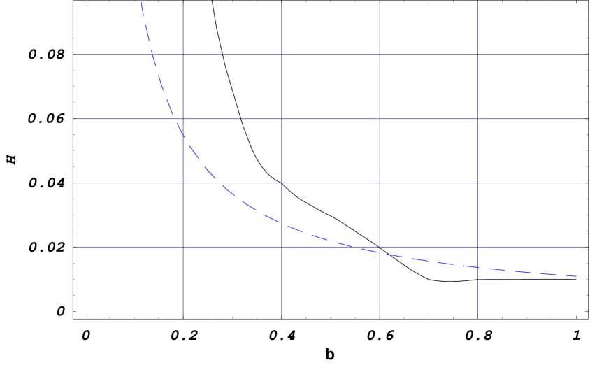
Figure 1: The dependence of the strengths of generated magnetic field ($H$) on inverse temperature ($b$). The dashed line is the theoretical position in the case of single magnetic field and the solid is calculated one in presence of both fields.

$\beta$	$x$	$\delta x$	$\delta x/x$, %	$\bar{x}$
0.1	0.7	$0.0000165$	$0.002$	$0.7000165$
0.2	0.2	$0.000745$	$0.373$	$0.200745$
0.3	0.07	$-0.0000549$	$-0.079$	$0.0699451$
0.4	0.04	$-0.0000358$	$-0.090$	$0.0399642$
0.5	0.03	$-0.0000467$	$-0.156$	$0.0299533$
0.6	0.02	$-0.0000492$	$-0.246$	$0.0199508$
0.7	0.01	$-0.0000380$	$-0.380$	$0.0099620$
0.8	0.01	$-0.0000619$	$-0.619$	$0.0099381$
0.9	0.01	$-0.0000241$	$-0.241$	$0.0099759$
1.0	0.01	$-0.0000357$	$-0.357$	$0.0099643$

Table 1. The strength of generated magnetic field.

As it is seen, the increase of inverse temperature leads to decreasing the strengths of generated fields. This dependence is well accorded with the picture of the universe cooling.

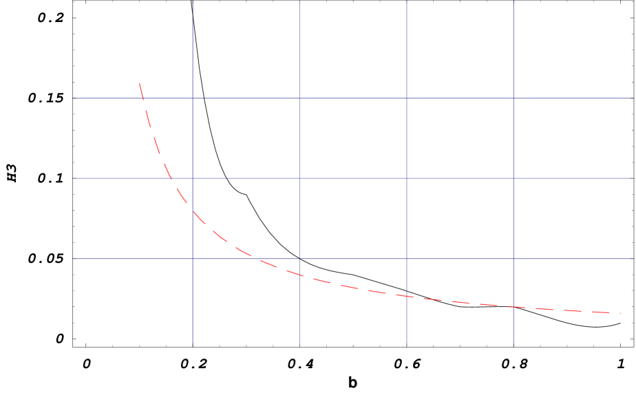
Figure 2: The dependence of the strengths of generated chromomagnetic field ($H3$) on inverse temperature ($b$). The dashed line is the theoretical position in the case of single chromomagnetic field and the solid one is calculated in the presence of both fields.

$\beta$	$y$	$\delta y$	$\delta y/y$, %	$\bar{y}$
0.1	0.8	$0.000301$	$0.038$	$0.800301$
0.2	0.2	$-0.000239$	$-0.119$	$0.199761$
0.3	0.09	$-0.0000988$	$-0.110$	$0.0899012$
0.4	0.05	$-0.0000884$	$-0.177$	$0.0499116$
0.5	0.04	$-0.000112$	$-0.280$	$0.039888$
0.6	0.03	$-0.0000982$	$-0.327$	$0.0299018$
0.7	0.02	$-0.0000442$	$-0.221$	$0.0199558$
0.8	0.02	$-0.0000733$	$-0.367$	$0.0199267$
0.9	0.01	$-0.000117$	$-1.166$	$0.009883$
1.0	0.01	$-0.000175$	$-1.749$	$0.009825$

Table 2. The strengths of generated chromomagnetic field.

From the above analysis it follows that at high temperatures the value of the each type magnetic field is increased when other one is taken into account. With temperature decreasing this effect becomes less pronounced and disappears at comparably low temperatures $\beta\sim 1$.

4 Discussion

Let us discuss the results obtained. As it was elaborated in the approximation to the EP including the one-loop and the daisy diagrams, in the SM at high temperatures both the magnetic and chromomagnetic fields have to be generated. These states are stable, as it follows from the absence of the imaginary terms in the EP minima.

If the quark loops are discarded, both of the fields can be generated in the system, separately. All these states are stable, due to magnetic mass $\sim g^{2}(gH)^{1/2}T$ of transversal gauge field modes. Here it worth to mention that the one-loop transversal gauge field mass is of order $\sim g^{4}T^{2}$ as nonperturbative calculations predict. This estimate is because the magnetic field strength of the spontaneously generated fields is of order $(gH)^{1/2}\sim g^{2}T$ Sta , Once . The possibility to calculate the magnetic mass in perturbation theory is due to the approach when an external field is taken into consideration exactly when the polarization operator of gauge field is calculated SkSt . If one accounts for the magnetic field perturbatively, zero value will be obtained Pers .

As it is seen from the Figures 1,2, presenting the results of numeric computations within the exact EP, the strengths of generated fields are increasing with the temperature rising. It is also found that the curves obtained in high temperature expansion of the EP Once are in good agreement with our numeric calculations.

The ground state possessing the magnetic and chromomagnetic fields makes advantage for existing of these fields in the electroweak transition epoch. The state with the fields is stable in the whole considered temperature interval. The imaginary part in the EP exists for the external fields much stronger then the strengths of the spontaneously generated ones. The interfusion of magnetic and chromomagnetic fields arisen from the quark sector of the EP is weak. The change of the field minima in inclusion of the fields mixing does not exceed $2$ per cents.

During the cooling of the universe the strengths of generated fields are decreasing that is in an agreement with what is expected in cosmology.

One of the consequences on the results obtained is the presence of strong chromomagnetic field in the early universe, in particular, at the electroweak phase transition and, probably, till the deconfinement temperature. Influence of this field on the transitions may bring new insight on these problems. As our estimate showed, the chromomagnetic field is as strong as magnetic one. So, the role of strong interactions in the early universe in the field presence needs more detailed investigations as compared to what is usually assumed Dar .

References

- (1) K.Enqvist, Int.J.Mod.Phys. D7, (1998) 331-350, astro-ph/9803196.
- (2) K.Enqvist, Invited Talk at the Strong and Electroweak Matter ’97, Hungary, astro-ph/9707300.
- (3) D.Grasso, H.R.Rubinstein, Phys.Rept. 348, (2001) 163-266, astro-ph/0009061 v.2.
- (4) K.Enquist, P.Olesen, Phys. Lett. B329, (1994) 195.
- (5) A.O.Starinets, A.S.Vshivtsev, V.Ch.Zhukovsky, Phys. Lett. 322, (1994) 403.
- (6) V.Skalozub, M.Bordag, Nucl.Phys. B576, (2000) 430.
- (7) G.K.Savvidy, Phys.Lett. 71B, (1977) 133.
- (8) M.Gionannini, M.Shaposhnikov, Phys.Rev. D57, (1998) 2186.
- (9) M.Joyce, M.Shaposhnikov, Phys. Rev.Lett. 79, (1997) 1192.
- (10) V.V.Skalozub, A.V.Strelchenko, Physics of Atomic Nuclei 63 No.11, (2000) 1956-1962.
- (11) Ta-Pie Cheng, Ling-Fong Li, Clarendon Press-Oxford, 1984.
- (12) V.V.Skalozub, Sov.J.Part.Nucl. 16, (1985) 445.
- (13) J.I. Kapusta, Cambridge university Press, (1989).
- (14) M.E.Carrington, Phys.Rev. D45, (1992) 2933.
- (15) J.Schwinger, Phys.Rev. 82 N5, (1951) 664.
- (16) A.Cabo, Fortschr.Phys. 29, (1981) 495.
- (17) Yu.Yu.Reznikov, V.V.Skalozub, Sov. J. Nucl. Phys. 46, (1987) 1085.
- (18) V.V.Skalozub, Int.J.Mod.Phys. A11, (1996) 5643.
- (19) V.Skalozub, M.Bordag, V.Demchik, hep-th/9912071.
- (20) P.Elmfors, D.Persson, Nucl.Phys. B538, (1999) 309-320, hep-ph/9806335 v.2.