January, 2002

Charmful Baryonic $B$ Decays $\bar{B}^{0}\to\Lambda_{c}\,\bar{p}$ and $\overline{B}\to\Lambda_{c}\,\bar{p}\,\pi(\rho)$

Hai-Yang Cheng^1,2,3 and Kwei-Chou Yang⁴

¹ Institute of Physics, Academia Sinica

Taipei, Taiwan 115, Republic of China

² Physics Department, Brookhaven National Laboratory

Upton, New York 11973

³ C.N. Yang Institute for Theoretical Physics, State University of New York

Stony Brook, New York 11794

⁴ Department of Physics, Chung Yuan Christian University

Chung-Li, Taiwan 320, Republic of China

Abstract

We study the two-body and three-body charmful baryonic $B$ decays: $\overline{B}^{0}\to\Lambda_{c}\,\bar{p}$ and $\overline{B}\to\Lambda_{c}\,\bar{p}\,\pi(\rho)$. The factorizable $W$-exchange contribution to $\overline{B}^{0}\to\Lambda_{c}\,\bar{p}$ is negligible. Applying the bag model to evaluate the baryon-to-baryon weak transition matrix element, we find ${\cal B}(\overline{B}^{0}\to\Lambda_{c}\,\bar{p}){\ \lower-1.2pt\vbox{\hbox{\hbox to0.0pt{$<$\hss}\lower 5.0pt\vbox{\hbox{$\sim$} }}}\ }1.1\times 10^{-5}|g_{B^{0}p\Sigma_{b}^{+}}/6|^{2}$ with $g_{B^{0}p\Sigma_{b}^{+}}$ being a strong coupling for the decay $\Sigma_{b}^{+}\to\overline{B}^{0}p$ and hence the predicted branching ratio is well below the current experimental limit. The factorizable contributions to $B^{-}\to\Lambda_{c}\,\bar{p}\pi^{-}$ can account for the observed branching ratio of order $6\times 10^{-4}$. The branching ratio of $B^{-}\to\Lambda_{c}\,\bar{p}\rho^{-}$ is larger than that of $B^{-}\to\Lambda_{c}\,\bar{p}\pi^{-}$ by a factor of about 2.6 . We explain why the three-body charmful baryonic $B$ decay has a larger rate than the two-body one, contrary to the case of mesonic $B$ decays.

I Introduction

Inspired by the claim of the observation of the decay modes $p\bar{p}\pi^{\pm}$ and $p\bar{p}\pi^{+}\pi^{-}$ in $B$ decays by ARGUS [2] in the late 1980s, baryonic $B$ decays were studied extensively around the early 1990s [3, 4, 5, 6, 7, 8, 9, 10, 11, 12, 13, 14] with the focus on the two-body decay modes, e.g. $B\to p\bar{p},~{}\Lambda\bar{\Lambda}$. Up to now, none of the two-body baryonic $B$ decays have been observed. Indeed, most of the earlier predictions based on the pole model or QCD sum rule or the diquark model are too large compared to experiment [15, 16] (see Table I).

TABLE I.: Predictions of branching ratios for some two-body baryonic $B$ decays in various models. We have normalized the branching ratios to $|V_{ub}/V_{cb}|=0.085\,$. The predictions given in [11] are carried out in two different quark-pair-creation models: local and nonlocal. Experimental limits are taken from [14,15].

					[11]
	[4]	[8]	[10]	[11]	non-local	local	experiment
$\overline{B}^{0}\to\Lambda_{c}\bar{p}$		$4\times 10^{-4}$	$8.5\times 10^{-4}$	$1.1\times 10^{-3}$	$1.7\times 10^{-3}$	$1.9\times 10^{-3}$	$<2.1\times 10^{-4}$
$\overline{B}^{0}\to p\bar{p}$	$4.2\times 10^{-6}$	$1.2\times 10^{-6}$	$5.9\times 10^{-6}$	$7.0\times 10^{-6}$	$2.9\times 10^{-6}$	$2.7\times 10^{-5}$	$<1.6\times 10^{-6}$
$\overline{B}^{0}\to\Lambda\bar{\Lambda}$			$3.0\times 10^{-6}$		$1.2\times 10^{-6}$	$2.3\times 10^{-5}$	$<2.3\times 10^{-6}$
$B^{-}\to\bar{\Delta}^{--}p$	$1.5\times 10^{-4}$	$2.9\times 10^{-7}$		$3.2\times 10^{-4}$	$7.2\times 10^{-7}$	$8.7\times 10^{-6}$	$<1.5\times 10^{-4}$

In order to understand why the momentum spectrum of produced $\Lambda_{c}$ in inclusive $B$ decays is soft and why the two-body decay modes, e.g. $\overline{B}\to\{\Lambda_{c},\Sigma_{c}\}\{\bar{p},\bar{\Delta}\}$, have not been observed, Dunietz [17] argued that a straightforward Dalitz plot for the dominant $b\to c\bar{u}d$ transition predicts the $c\,d$ invariant mass to be very large. The very massive $c\,d\,q$ objects would be usually seen as $\Lambda_{c}n\pi(n\geq 1)$ if the $c\,d$ forms a charmed baryon. This explains the observed soft $\Lambda_{c}$ momentum spectrum and the non-observation of $\Lambda_{c}\bar{p}$ decay. Since the very massive $c\,d\,q$ could also be seen as $D^{(*)}NX$, the baryonic processes $\overline{B}\to D^{(*)}N\bar{N}^{\prime}X$ would be likely sizable. Indeed, CLEO has recently reported the observation of $B^{0}\to D^{*-}p\bar{n}$ at the $10^{-3}$ level and $B^{0}\to D^{*-}p\bar{p}\pi^{+}$ at the $10^{-4}$ level [18]. Theoretically, the three-body decay modes $B\to D^{*-}N\bar{N}$ and $B^{0}\to\rho^{-}(\pi^{-})p\bar{n}$ have been recently studied in [19, 20].

A similar observation has been made by Hou and Soni [21]. They pointed out that the smallness of the two-body baryonic decay $B\to{\cal B}_{1}\overline{\cal B}_{2}$ has to do with the large energy release. They conjectured that in order to have larger baryonic $B$ decays, one has to reduce the energy release and at the same time allow for baryonic ingredients to be present in the final state. Under this argument, the three-body decay, for example $B\to\rho p\bar{n}$, will dominate over the two-body mode $B\to p\bar{p}$ since the ejected $\rho$ meson in the former decay carries away much energy and the configuration is more favorable for baryon production because of reduced energy release compared to the latter [20]. This is in contrast to the mesonic $B$ decays where two-body decay rates are usually comparable to the three-body modes. The large rate of $B^{0}\to D^{*-}p\bar{n}$ and $B^{0}\to D^{*-}p\bar{p}\pi^{+}$ observed by CLEO indicates that the decays $B\to$ baryons receive comparable contributions from $\overline{B}\to\Lambda_{c}\bar{p}X$ and $\overline{B}\to[D]N\bar{N}^{\prime}X$, where $[D]$ denotes any charmed meson. By the same token, it is expected that for charmless baryonic $B$ decays, $\overline{B}\to\rho(\pi){\cal B}_{1}\overline{\cal B}_{2}$ are the dominant modes induced by tree operators and $\overline{B}\to(\pi,\eta^{\prime},\rho){\cal B}_{1(s)}\overline{B}_{2}$, e.g. $\overline{B}\to\rho\Lambda\bar{p}$, are the leading modes induced by penguin diagrams.

In this work we focus on charmful baryonic decays $\overline{B}\to\Lambda_{c}\bar{p}X$. The experimental results are summarized as [22]:

$${\cal B}(B^{-}\to\Lambda_{c}\bar{p}\pi^{-})=(6.2\pm 2.7)\times 10^{-4}, \qquad{\cal B}(\overline{B}^{0}\to\Lambda_{c}\bar{p}\pi^{0})<5.9\times 10^{-4},$$ (1)

$${\cal B}(\overline{B}^{0}\to\Lambda_{c}\bar{p}\pi^{+}\pi^{-})=(1.3\pm 0.6)\times 10^{-3}, \qquad{\cal B}(B^{-}\to\Lambda_{c}\bar{p}\pi^{-}\pi^{0})<3.12\times 10^{-3},$$ (2)

together with the upper limit ${\cal B}(\overline{B}^{0}\to\Lambda_{c}\bar{p})<2.1\times 10^{-4}$. It is evident that the two-body mode is suppressed. Specifically, we shall study $\overline{B}^{0}\to\Lambda_{c}\,\bar{p}$ and $B^{-}\to\Lambda_{c}\,\bar{p}\,\pi^{-}(\rho^{-})$ in detail in order to understand their underlying decay mechanism. It has been advocated that the $B$ decay to $\Lambda_{c}\bar{p}+\pi$’s is suppressed relative to $\Lambda_{c}\bar{p}$ [11]. We shall see that this is not the case.

The layout of the present paper is organized as follows. In Sec. II we first study the two-body charmful decay $\overline{B}^{0}\to\Lambda_{c}\,\bar{p}$ to update the prediction of its branching ratio. We then turn to the three-body decays $\overline{B}\to\Lambda_{c}\,\bar{p}\,\pi(\rho)$ in Sec. III. A detail of the MIT bag model for the evaluation of baryon-to-baryon weak transition matrix elements is presented in the Appendix.

II Two-body charmful baryonic decay $\overline{B}^{0}\to\Lambda_{c}\,\bar{p}$

We first study the two-body baryonic decay $\overline{B}^{0}\to\Lambda_{c}\,\bar{p}$ to update its prediction and understand why it is suppressed compared to three-body modes. To proceed, we first write down the relevant Hamiltonian

$${\cal H}_{\rm eff} = {G_{F}\over\sqrt{2}}V_{cb}V_{ud}^{*}[c_{1}(\mu)O_{1}(\mu)+c_{2}(\mu)O_{2}(\mu)]+h.c.,$$ (3)

where $O_{1}=(\bar{c}b)(\bar{d}u)$ and $O_{2}=(\bar{c}u)(\bar{d}b)$ with $(\bar{q}_{1}q_{2})\equiv\bar{q}_{1}\gamma_{\mu}(1-\gamma_{5})q_{2}$. In order to ensure that the physical amplitude is renormalization scale and $\gamma_{5}$-scheme independent, we include vertex corrections to hadronic matrix elements. This amounts to modifying the Wilson coefficients by [23]:

$$c_{1}(\mu)\to c_{1}^{\rm eff} = c_{1}(\mu)+{\alpha_{s}\over 4\pi}\left(\gamma^{(0)T}\ln{m_{b}\over\mu}+\hat{r}^{T}\right)_{1i}c_{i}(\mu),$$ (4)

$$c_{2}(\mu)\to c_{2}^{\rm eff} = c_{2}(\mu)+{\alpha_{s}\over 4\pi}\left(\gamma^{(0)T}\ln{m_{b}\over\mu}+\hat{r}^{T}\right)_{2i}c_{i}(\mu),$$ (5)

where the anomalous dimension matrix $\gamma^{(0)}$ and the constant matrix $\hat{r}$ in the naive dimensional regularization and ’t Hooft-Veltman schemes can be found in [23]. The superscript $T$ in Eq. (4) denotes a transpose of the matrix. Numerically we have $c_{1}^{\rm eff}=1.168$ and $c_{2}^{\rm eff}=-0.365$ [23]. It should be stressed that $c_{1}^{\rm eff}$ and $c_{2}^{\rm eff}$ are renormalization scale and scheme independent. For later purposes we write

$${\cal H}_{\rm eff} = {G_{F}\over\sqrt{2}}V_{cb}V_{ud}^{*}[c_{+}O_{+}+c_{-}O_{-}]+h.c.,$$ (6)

with $O_{\pm}=O_{1}\pm O_{2}$ and $c_{\pm}={1\over 2}(c_{1}^{\rm eff}\pm c_{2}^{\rm eff})$.

The decay amplitude of $\overline{B}^{0}\to\Lambda_{c}\,\bar{p}$ consists of factorizable and nonfactorizable parts:

$$A(\overline{B}^{0}\to\Lambda_{c}\,\bar{p})=A(\overline{B}^{0}\to\Lambda_{c}\,\bar{p})_{\rm fact}+A(\overline{B}^{0}\to\Lambda_{c}\,\bar{p})_{\rm nonfact},$$ (7)

with

$$A(\overline{B}^{0}\to\Lambda_{c}\,\bar{p})_{\rm fact}={G_{F}\over\sqrt{2}}V_{cb}V_{ud}^{*}\,a_{2}\langle\Lambda_{c}\bar{p}|(\bar{c}u)|0\rangle\langle 0|(\bar{d}b)|\overline{B}^{0}\rangle,$$ (8)

where $a_{2}=c_{2}^{\rm eff}+c_{1}^{\rm eff}/N_{c}$. The short-distance factorizable contribution is nothing but the $W$-exchange diagram. This $W$-exchange contribution has been estimated and is found to be very small and hence can be neglected [6, 14]. However, a direct evaluation of nonfactorizable contributions is very difficult. This is the case in particular for baryons, which being made out of three quarks, in contrast to two quarks for mesons, bring along several essential complications. In order to circumvent this difficulty, it is customary to assume that the nonfactorizable effect is dominated by the pole diagram with low-lying baryon intermediate states; that is, nonfactorizable $s$- and $p$-wave amplitudes are dominated by ${1\over 2}^{-}$ low-lying baryon resonances and ${1\over 2}^{+}$ ground-state intermediate states, respectively [11]. For $\overline{B}^{0}\to\Lambda_{c}\,\bar{p}$, we consider the strong-interaction process $\overline{B}^{0}\to\Sigma_{b}^{+(*)}\,\bar{p}$ followed by the weak transition $\Sigma_{b}^{+(*)}\to\Lambda_{c}$, where $\Sigma_{b}^{*}$ is a ${1\over 2}^{-}$ baryon resonance (see Fig. 1). Considering the strong coupling

$$ig_{Bp\Sigma_{b}}\overline{\psi}_{\Sigma_{b}}\gamma_{5}\psi_{p}\phi_{B}+g_{Bp\Sigma_{b}^{*}}\overline{\psi}_{\Sigma_{b}^{*}}\psi_{p}\phi_{B},$$ (9)

the pole-diagram amplitude has the form

$$A(\overline{B}^{0}\to\Lambda_{c}\bar{p})_{\rm nonfact}=\bar{u}_{\Lambda_{c}}(A+B\gamma_{5})v_{p},$$ (10)

where

$$A=-{g_{B^{0}p\Sigma_{b}^{+*}}b_{\Sigma_{b}^{*}\Lambda_{c}}\over m_{\Lambda_{c}}-m_{\Sigma_{b}^{*}}},\qquad\qquad B=\,{g_{B^{0}p\Sigma_{b}^{+}}a_{\Sigma_{b}\Lambda_{c}}\over m_{\Lambda_{c}}-m_{\Sigma_{b}}}$$ (11)

correspond to $s$-wave parity-violating (PV) and $p$-wave parity-conserving (PC) amplitudes, respectively, and

$$\langle\Lambda_{c}|{\cal H}_{\rm eff}^{\rm PC}|\Sigma_{b}^{+}\rangle=\bar{u}_{\Lambda_{c}}a_{\Sigma_{b}\Lambda_{c}}u_{\Sigma_{b}},\qquad\quad\langle\Lambda_{c}|{\cal H}_{\rm eff}^{\rm PV}|\Sigma_{b}^{*+}\rangle=i\bar{u}_{\Lambda_{c}}b_{\Sigma_{b}^{*}\Lambda_{c}}u_{\Sigma_{b}^{*}}.$$ (12)

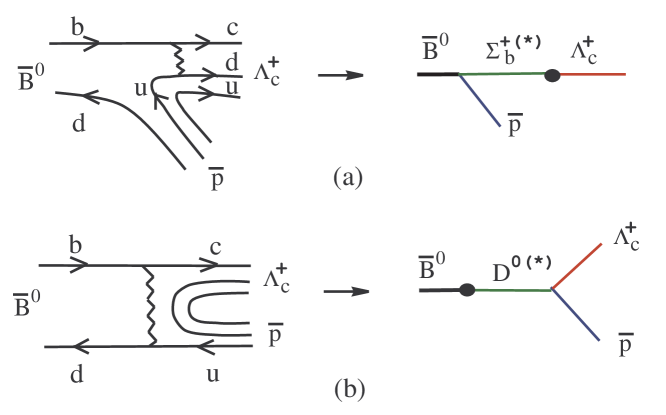
FIG. 1.: Some pole diagrams for $\overline{B}^{0}\to\Lambda_{c}\bar{p}$ where the symbol $\bullet$ denotes the weak vertex. (a) corresponds to nonfactorizable internal $W$ emission, while (b) to the $W$-exchange contribution.

The main task is to evaluate the weak matrix elements and the strong coupling constants. We shall employ the MIT bag model [24] to evaluate the baryon matrix elements (see e.g. [25, 26] for the method). Since the quark-model wave functions best resemble the hadronic states in the frame where both baryons are static, we thus adopt the static bag approximation for the calculation. Note that because the four-quark operator $O_{+}$ is symmetric in color indices, it does not contribute to the baryon-baryon matrix element since the baryon-color wave function is totally antisymmetric. From Eq. (6) and the Appendix we obtain the PC matrix element

$$a_{\Sigma_{b}\Lambda_{c}}=-{G_{F}\over\sqrt{2}}V_{cb}V_{ud}^{*}\,c_{-}{4\over\sqrt{6}}(X_{1}+3X_{2})(4\pi),$$ (13)

where

$$X_{1} = \int^{R}_{0}r^{2}dr[u_{c}(r)v_{u}(r)-v_{c}(r)u_{u}(r)][u_{d}(r)v_{b}(r)-v_{d}(r)u_{b}(r)],$$ (14)

$$X_{2} = \int^{R}_{0}r^{2}dr[u_{c}(r)u_{u}(r)+v_{c}(r)v_{u}(r)][u_{d}(r)u_{b}(r)+v_{d}(r)v_{b}(r)],$$ (15)

are four-quark overlap bag integrals (see the Appendix for notation). In principle, one can also follow [25] to tackle the low-lying negative-parity $\Sigma_{b}^{*}$ state in the bag model and evaluate the PV matrix element $b_{\Sigma^{*}_{c}\Lambda_{c}}$. However, it is known that the bag model is less successful even for the physical non-charm and non-bottom ${1\over 2}^{-}$ resonances [24], not mentioning the charm or bottom ${1\over 2}^{-}$ resonances. In short, we know very little about the ${1\over 2}^{-}$ state. Therefore, we will not evaluate the PV matrix element $b_{\Sigma_{b}^{*}\Lambda_{c}}$ as its calculation in the bag model is much involved and is far more uncertain than the PC one [25].

Using the bag wave functions given in the Appendix, we find, numerically,

$$X_{1}=-1.49\times 10^{-5}\,{\rm GeV}^{3},\qquad\quad X_{2}=1.81\times 10^{-4}\,{\rm GeV}^{3}.$$ (16)

The decay rate of $B\to{\cal B}_{1}\overline{\cal B}_{2}$ is given by

$$\Gamma(B\to{\cal B}_{1}\overline{\cal B}_{2}) = {p_{c}\over 4\pi}\Bigg{\{}|A|^{2}\,{(m_{B}+m_{1}+m_{2})^{2}p_{c}^{2}\over(E_{1}+m_{1})(E_{2}+m_{2})m_{B}^{2}}$$ (17)

$$+ |B|^{2}\,{[(E_{1}+m_{1})(E_{2}+m_{2})+p_{c}^{2}]^{2}\over(E_{1}+m_{1})(E_{2}+m_{2})m_{B}^{2}}\Bigg{\}},$$ (18)

where $p_{c}$ is the c.m. momentum, and $E_{i}$ and $m_{i}$ are the energy and mass of the baryon ${\cal B}_{i}$, respectively. Putting everything together we obtain

$${\cal B}(\overline{B}^{0}\to\Lambda_{c}\bar{p})_{\rm PC}=7.2\times 10^{-6}\left|{g_{B^{0}p\Sigma_{b}^{+}}\over 6}\right|^{2}.$$ (19)

The PV contribution is expected to be smaller. For example, it is found to be $\Gamma^{\rm PV}/\Gamma^{\rm PC}=0.59$ in [11]. Therefore, we conclude that

$${\cal B}(\overline{B}^{0}\to\Lambda_{c}\bar{p}){\ \lower-1.2pt\vbox{\hbox{\hbox to0.0pt{$<$\hss}\lower 5.0pt\vbox{\hbox{$\sim$} }}}\ }1.1\times 10^{-5}\left|{g_{B^{0}p\Sigma_{b}^{+}}\over 6}\right|^{2}.$$ (20)

The strong coupling $g_{B^{0}p\Sigma_{b}^{+}}$ has been estimated in [11] using the quark-pair-creation model and it is found to lie in the range $g_{B^{0}p\Sigma_{b}^{+}}=-(6\sim 10)$, recalling that $g_{\pi NN}\approx 14$. We shall see in Sec. III.A that the measurement of $B^{-}\to\Lambda_{c}\bar{p}\pi^{-}$ can be used to extract the coupling $g_{B^{+}p\Lambda_{b}}$ which in turn provides information on $g_{B^{0}p\Sigma_{b}^{+}}$. At any rate, the prediction (20) is consistent with the current experimental limit $2.1\times 10^{-4}$ [22]. Note that all earlier predictions based on the QCD sum rule [8] or the pole model [11] or the diquark model [12] are too large compared to experiment (see Table I). In the pole-model calculation in [11], the weak matrix element is largely overestimated.

III Three-body charmful baryonic decays

A $B^{-}\to\Lambda_{c}\,\bar{p}\,\pi^{-}$

The quark diagrams and the corresponding pole diagrams for $B^{-}\to\Lambda_{c}\,\bar{p}\,\pi^{-}$ are shown in Fig. 2. There exist two distinct internal $W$ emissions and only one of them is factorizable, namely Fig. 2(b). The external $W$ emission diagram Fig. 2(a) is of course factorizable. Therefore, unlike the two-body decay $\overline{B}^{0}\to\Lambda_{c}\bar{p}$, the three-body mode $B^{-}\to\Lambda_{c}\,\bar{p}\,\pi^{-}$ does receive sizable factorizable contributions

$$A(B^{-}\to\Lambda_{c}\bar{p}\pi^{-})_{\rm fact} = {G_{F}\over\sqrt{2}}V_{cb}V_{ud}^{*}\Big{\{}a_{1}\langle\pi^{-}|(\bar{d}u)|0\rangle\langle\Lambda_{c}\bar{p}|(\bar{c}b)|B^{-}\rangle$$ (21)

$$+ a_{2}\langle\pi^{-}|(\bar{d}b)|B^{-}\rangle\langle\Lambda_{c}\bar{p}|(\bar{c}u)|0\rangle\Big{\}}\equiv A_{1}+A_{2},$$ (22)

where naively $a_{1}=c_{1}^{\rm eff}+c_{2}^{\rm eff}/N_{c}$ and $a_{2}=c_{2}^{\rm eff}+c_{1}^{\rm eff}/N_{c}$, to which we will come back later. Unfortunately, in practice we do not know how to evaluate the 3-body hadronic matrix element $\langle\Lambda_{c}\bar{p}|(\bar{c}b)|B^{-}\rangle$. Thus we will instead evaluate the corresponding low-lying pole diagrams for external $W$-emission, namely, the strong process $B^{-}\to\Lambda_{b}^{(*)}\bar{p}$, followed by the weak decay $\Lambda_{b}^{(*)}\to\Lambda_{c}\pi^{-}$ [see Fig. 2(a)]. Its amplitude is given by

$$A_{1} = -{G_{F}\over\sqrt{2}}V_{ud}V_{cb}^{*}\,g_{B^{+}p\Lambda_{b}}f_{\pi}\,a_{1}\,\bar{u}_{\Lambda_{c}}\Big{\{}f_{1}^{\Lambda_{b}\Lambda_{c}}(m_{\pi}^{2})[2p_{\pi}\cdot p_{\Lambda_{c}}+p\!\!\!/_{\pi}(m_{\Lambda_{b}}-m_{\Lambda_{c}})]\gamma_{5}$$ (24)

$$+g_{1}^{\Lambda_{b}\Lambda_{c}}(m_{\pi}^{2})[2p_{\pi}\cdot p_{\Lambda_{c}}-p\!\!\!/_{\pi}(m_{\Lambda_{b}}+m_{\Lambda_{c}})]\Big{\}}v_{\bar{p}}\times{1\over(p_{\Lambda_{c}}+p_{\pi})^{2}-m_{\Lambda_{b}}^{2}},$$

where we have applied factorization to the weak decay $\Lambda_{b}\to\Lambda_{c}\pi$ and employed the form factors defined by

$$\langle\Lambda_{c}^{+}(p_{\Lambda_{c}})|(\bar{c}b)|\Lambda_{b}^{0}(p_{\Lambda_{b}})\rangle = \bar{u}_{\Lambda_{c}}\Bigg{\{}f_{1}^{\Lambda_{b}\Lambda_{c}}(p_{\pi}^{2})\gamma_{\mu}+i{f_{2}^{\Lambda_{b}\Lambda_{c}}(p_{\pi}^{2})\over m_{\Lambda_{b}}}\sigma_{\mu\nu}p_{\pi}^{\nu}+{f_{3}^{\Lambda_{b}\Lambda_{c}}(p_{\pi}^{2})\over m_{\Lambda_{b}}}p_{\pi\mu}$$ (26)

$$-[g_{1}^{\Lambda_{b}\Lambda_{c}}(p_{\pi}^{2})\gamma_{\mu}+i{g_{2}^{\Lambda_{b}\Lambda_{c}}(p_{\pi}^{2})\over m_{\Lambda_{b}}}\sigma_{\mu\nu}p_{\pi}^{\nu}+{g_{3}^{\Lambda_{b}\Lambda_{c}}(p_{\pi}^{2})\over m_{\Lambda_{b}}}p_{\pi\mu}]\gamma_{5}\Bigg{\}}u_{\Lambda_{b}},$$

where $p_{\pi}=p_{\Lambda_{b}}-p_{\Lambda_{c}}$. Note that the ${1\over 2}^{-}$ intermediate state $\Lambda_{b}^{*}$ makes no contribution as the matrix element $\langle\Lambda_{c}|(\bar{c}b)|\Lambda_{b}^{*}\rangle$ vanishes. Likewise, the intermediate states $\Sigma_{b}^{0}$ and $\Sigma_{b}^{0*}$ also do not contribute to $A_{1}$ under the factorization approximation because the weak transition $\langle\Lambda_{c}|(\bar{c}b)|\Sigma_{b}^{0(*)}\rangle$ is prohibited as $\Sigma_{b}$ and $\Sigma_{b}^{*}$ are sextet bottom baryons whereas $\Lambda_{c}$ is a anti-triplet charmed baryon.

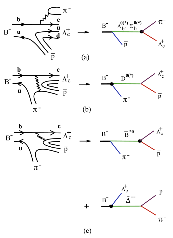
FIG. 2.: Some pole diagrams for $B^{-}\to\Lambda_{c}\bar{p}\pi^{-}$ where the symbol $\bullet$ denotes the weak vertex. (a) and (b) correspond to factorizable external and internal $W$-emission contributions, respectively, while (c) to nonfactorizable internal $W$-emission diagrams. There are two pole diagrams corresponding to the quark diagram in (c).

To evaluate the fcatorizable amplitude $A_{2}$, as shown in Fig. 2(b), we apply the parametrization for the $B-\pi$ matrix element

$$\langle\pi^{-}(p_{\pi})|(\bar{d}b)|B^{-}(p_{B})\rangle=F_{1}^{B\pi}(q^{2})(p_{B}+p_{\pi})_{\mu}+\left(F_{0}^{B\pi}(q^{2})-F_{1}^{B\pi}(q^{2})\right){m_{B}^{2}-m_{\pi}^{2}\over q^{2}}q_{\mu},$$ (27)

and obtain

$$A_{2}={G_{F}\over\sqrt{2}}V_{ud}V_{cb}^{*}\,a_{2}\bar{u}_{\Lambda_{c}}\left[(ap\!\!\!/_{\pi}+b)-(cp\!\!\!/_{\pi}+d)\gamma_{5}\right]v_{p},$$ (28)

where

$$a = 2f_{1}^{\Lambda_{c}p}(t)F_{1}^{B\pi}(t)+2f_{2}^{\Lambda_{c}p}(t)F_{1}^{B\pi}(t)(m_{\Lambda_{c}}+m_{p})/m_{\Lambda_{c}},$$ (29)

$$b = (m_{\Lambda_{c}}-m_{p})f_{1}^{\Lambda_{c}p}(t)\left[F_{1}^{B\pi}(t)+(F^{B\pi}_{0}(t)-F^{B\pi}_{1}(t)){m_{B}^{2}-m_{\pi}^{2}\over t}\right]$$ (31)

$$-2f_{2}^{\Lambda_{c}p}(t)F_{1}^{B\pi}(t)(p_{\Lambda_{c}}-p_{p})\cdot p_{\pi}/m_{\Lambda_{c}}+f_{3}^{\Lambda_{c}p}(t)F_{0}^{B\pi}(t)(m_{B}^{2}-m_{\pi}^{2})/m_{\Lambda_{c}},$$

$$c = 2g_{1}^{\Lambda_{c}p}(t)F_{1}^{B\pi}(t)+2g_{2}^{\Lambda_{c}p}(t)F_{1}^{B\pi}(t)(m_{\Lambda_{c}}-m_{p})/m_{\Lambda_{c}},$$ (32)

$$d = (m_{\Lambda_{c}}+m_{p})g_{1}^{\Lambda_{c}p}(t)\left[F_{1}^{B\pi}(t)+(F^{B\pi}_{0}(t)-F^{B\pi}_{1}(t)){m_{B}^{2}-m_{\pi}^{2}\over t}\right]$$ (34)

$$-2g_{2}^{\Lambda_{c}p}(t)F_{1}^{B\pi}(t)(p_{\Lambda_{c}}-p_{p})\cdot p_{\pi}/m_{\Lambda_{c}}+g_{3}^{\Lambda_{c}p}(t)F_{0}^{B\pi}(t)(m_{B}^{2}-m_{\pi}^{2})/m_{\Lambda_{c}},$$

and $t\equiv q^{2}=(p_{B}-p_{\pi})^{2}=(p_{\Lambda_{c}}+p_{p})^{2}$.

The form factors $f_{i}$ and $g_{i}$ for the heavy-to-heavy and heavy-to-light baryonic transitions at zero recoil have been computed using the non-relativistic quark model [27]. In principle, HQET puts some constraints on these form factors. However, it is clear that HQET is not adequate for our purposes: the predictive power of HQET for the baryon form factors at order $1/m_{Q}$ is limited only to the antitriplet-to-antitriplet heavy baryonic transition. Hence, we will follow [27] to apply the nonrelativistic quark model to evaluate the weak current-induced baryon form factors at zero recoil in the rest frame of the heavy parent baryon, where the quark model is most trustworthy. This quark model approach has the merit that it is applicable to heavy-to-heavy and heavy-to-light baryonic transitions at maximum $q^{2}$ and that it becomes meaningful to consider $1/m_{q}$ corrections as long as the recoil momentum is smaller than the $m_{q}$ scale. It has been shown in [27] that the quark model predictions agree with HQET for the antitriplet-to-antitriplet (e.g., $\Lambda_{b}\to\Lambda_{c},~{}\Xi_{b}\to\Xi_{c}$) form factors to order $1/m_{Q}$. For sextet $\Sigma_{b}\to\Sigma_{c}$ and $\Omega_{b}\to\Omega_{c}$ transitions, the quark-model results are also in accord with the HQET predictions (for details see [28]). Numerically we have [28]

$$f_{1}^{\Lambda_{b}\Lambda_{c}}(q^{2}_{m})=g_{1}^{\Lambda_{b}\Lambda_{c}}(q^{2}_{m})=1.02,\quad f_{2}^{\Lambda_{b}\Lambda_{c}}(q^{2}_{m})=g_{3}^{\Lambda_{b}\Lambda_{c}}(q^{2}_{m})=-0.23,$$ (35)

$$f_{3}^{\Lambda_{b}\Lambda_{c}}(q^{2}_{m})=g_{2}^{\Lambda_{b}\Lambda_{c}}(q^{2}_{m})=-0.03,$$ (36)

for the $\Lambda_{b}-\Lambda_{c}$ transition at zero recoil $q_{m}^{2}=(m_{\Lambda_{b}}-m_{\Lambda_{c}})^{2}$, and [27]

$$f_{1}^{\Lambda_{c}p}(q^{2}_{m})=g_{1}^{\Lambda_{c}p}(q^{2}_{m})=0.80,\quad f_{2}^{\Lambda_{c}p}(q^{2}_{m})=g_{3}^{\Lambda_{c}p}(q^{2}_{m})=-0.21,$$ (37)

$$f_{3}^{\Lambda_{c}p}(q^{2}_{m})=g_{2}^{\Lambda_{c}p}(q^{2}_{m})=-0.07,$$ (38)

for the $\Lambda_{c}-p$ transition at $q^{2}_{m}=(m_{\Lambda_{c}}-m_{p})^{2}$.

Since the calculation for the $q^{2}$ dependence of form factors is beyond the scope of the non-relativistic quark model, we will follow the conventional practice to assume a pole dominance for the form-factor $q^{2}$ behavior:

$$f(q^{2})=f(q^{2}_{m})\left({1-q^{2}_{m}/m^{2}_{V}\over 1-q^{2}/m_{V}^{2}}\right)^{n}\,,\qquad g(q^{2})=g(q^{2}_{m})\left({1-q^{2}_{m}/m^{2}_{A}\over 1-q^{2}/m_{A}^{2}}\right)^{n}\,,$$ (39)

where $m_{V}$ ($m_{A}$) is the pole mass of the vector (axial-vector) meson with the same quantum number as the current under consideration. The function

$$G(q^{2})=\left({1-q^{2}_{m}/m^{2}_{\rm pole}\over 1-q^{2}/m_{\rm pole}^{2}}\right)^{n}$$ (40)

plays the role of the baryon Isgur-Wise function $\zeta(\omega)$ for the $\Lambda_{Q}\to\Lambda_{Q^{\prime}}$ transition, namely, $G=1$ at $q^{2}=q^{2}_{m}$. The function $\zeta(\omega)$ has been calculated in the literature in various different models [29, 30, 31, 32, 33, 34]. Using the pole masses $m_{V}=6.34$ GeV, $m_{A}=6.73$ GeV for the $\Lambda_{b}\to\Lambda_{c}$ transition, it is found that $G(q^{2})$ is consistent with the earlier soliton model [29] and MIT bag model [30] calculation of $\zeta(\omega)$ for $n=2$ [27]. However, a recent calculation of $\zeta(\omega)$ in [34] yields

$$\zeta(\omega)=\left({2\over 1+\omega}\right)^{1.23+0.4/\omega}$$ (41)

and this favors $n=1$. Therefore, whether the $q^{2}$ dependence is monopole or dipole for heavy-to-heavy transitions is not clear. Hence we shall use both monopole and dipole dependence in ensuing calculations. Moreover, one should bear in mind that the $q^{2}$ behavior of form factors is probably more complicated and it is likely that a simple pole dominance only applies to a certain $q^{2}$ region, especially for the heavy-to-light transition. For the $\Lambda_{c}-p$ transition, we will use the pole masses $m_{V}=2.01$ GeV and $m_{A}=2.42$ GeV and assume dipole $q^{2}$ dependence.

For the form factors $F_{0,1}^{B\pi}(q^{2})$ we consider the recently proposed Melikhov-Stech (MS) model based on the constituent quark picture [35]. Although the form factor $q^{2}$ dependence is in general model dependent, it should be stressed that $F_{1}^{B\pi}(q^{2})$ increases with $q^{2}$ more rapidly than $F_{0}^{B\pi}(q^{2})$ as required by heavy quark symmetry. We shall see below that the predicted decay rates are insensitive to the choice of form-factor models.

Thus far we have only discussed factorizable contributions. The nonfactorizable effects are conventionally estimated by evaluating the corresponding pole diagrams. The processes

$$B^{-}\to\pi^{-}+ \overline{B}^{*0}$$ (42)

$$\hookrightarrow \bar{p}+\Lambda_{c}$$ (43)

$$B^{-}\to\Lambda_{c}+ \bar{\Delta}^{--}$$ (44)

$$\hookrightarrow \bar{p}+\pi^{-}$$ (45)

are some examples of the pole diagrams shown in Figs. 2(c) and 2(d); they correspond to nonfactorizable internal $W$-emission. Presumably these nonfactorizable contributions will affect the parameter $a_{2}$ substantially.

The total decay rate for the process $B^{-}(p_{B})\to\Lambda_{c}(p_{1})+\bar{p}(p_{2})+\pi^{-}(p_{3})$ is computed by

$$\Gamma={1\over(2\pi)^{3}}\,{1\over 32m_{B}^{3}}\int|A|^{2}dm_{12}^{2}dm_{23}^{2},$$ (46)

or

$$\Gamma={1\over(2\pi)^{3}}\,{1\over 16m_{B}^{2}}\int|A|^{2}dE_{\pi}dm_{23}^{2},$$ (47)

where $E_{\pi}$ is the energy of the outgoing pion, and $m_{ij}^{2}=(p_{i}+p_{j})^{2}$ with $p_{3}=p_{\pi}$. For a given $E_{\pi}$, the range of $m_{23}^{2}$ is fixed by kinematics. Under naive factorization, the parameter $a_{2}$ appearing in Eq. (21) is numerically equal to 0.024, which is very small compared to the value of $a_{2}=0.40-0.55$ extracted from $\overline{B}^{0}\to D^{0(*)}\pi^{0}$ decays [36] and $|a_{2}|=0.26\pm 0.02$ in $B\to{J/\psi}K$ decay [37]. As stated before, $a_{2}$ may receive sizable contributions from nonfactorizable pole diagrams Figs. 2(c) and 2(d). Therefore, we will treat $a_{2}$ as a free parameter and take $a_{2}=0.30$ as an illustration. For strong coupling constants a simple quark-pair-creation model yields (see Appendix C of [11] for detail)

$$|g_{B^{+}p\Lambda_{b}}|=3\sqrt{3/2}\,|g_{B^{0}p\Sigma_{b}^{+}}|.$$ (48)

Hence, the strong coupling constant $|g_{B^{+}p\Lambda_{b}}|$ is much larger than $|g_{B^{0}p\Sigma_{b}^{+}}|$. Putting everything together we obtain numerically

$${\cal B}(B^{-}\to\Lambda_{c}\bar{p}\pi^{-}) = \cases{(10.0r^{2}+0.04-0.8r)\times 10^{-4}&for~{}$n=1$\cr(5.5r^{2}+0.04-0.6r)\times 10^{-4}&for~{}$n=2$}$$ (49)

$$= \cases{9.2\times 10^{-4}&for~{}$n=1$~{}and~{}$g_{B^{+}p\Lambda_{b}}=16$\cr 4.9\times 10^{-4}&for~{}$n=2$~{}and~{}$g_{B^{+}p\Lambda_{b}}=16$},$$ (50)

where $r=g_{B^{+}p\Lambda_{b}}/16$ and the first two lines show explicitly the contributions from external $W$-emission, internal $W$-emission and their interference, respectively. We find that the external $W$-emission and internal $W$-emission contribute destructively (constructively) if the $\Lambda_{c}-p$ baryonic form factor $q^{2}$ dependence is of the dipole (monopole) form. From Eq. (49) we find that the strong coupling constant $g_{B^{+}p\Lambda_{b}}$ in the vicinity of order 16 can accommodate the observed branching ratio of $B^{-}\to\Lambda_{c}\bar{p}\pi^{-}$ [see Eq. (1)]. It follows from Eq. (48) that $|g_{B^{0}p\Sigma_{b}^{+}}|\sim 4.3$, which is close to the model estimate of $6\sim 10$ given in [11]. It is likely that the quark-pair-creation-model calculation of strong couplings is more reliable for their ratios than their absolute values.

We have checked explicitly that the results are fairly insensitive to the choice of $B-\pi$ form factors. For example, we have computed the branching ratios using the three different form-factor models given in [38] and found that the difference in rates is at most at the level of 5%.

Evidently, the calculated branching ratios are in agreement with experiment (1). There are several reasons why the three-body decay rate of $B^{-}\to\Lambda_{c}\bar{p}\pi^{-}$ is larger than that of the two-body one $\overline{B}^{0}\to\Lambda_{c}\bar{p}$. (i) The former decay receives external and internal $W$-emission contributions, whereas the color-suppressed factorizable $W$-exchange contribution to the latter is greatly suppressed. (ii) At the pole-diagram level, the $\Sigma_{b}$ propagator in the pole amplitude for the latter is of order $1/(m_{b}^{2}-m_{c}^{2})$, while the invariant mass of the $(\Lambda_{c}\bar{p})$ system can be large enough in the former decay so that its propagator in the pole diagram is not subject to the same $1/m_{b}^{2}$ suppression. (iii) The strong coupling constant for $\Lambda_{b}\to B^{-}p$ is larger than that for $\Sigma_{b}^{+}\to\overline{B}^{0}p$.

B $B^{-}\to\Lambda_{c}\,\bar{p}\,\rho^{-}$

Naively it is expected that $\Lambda_{c}\bar{p}\rho^{-}$ has a larger rate than $\Lambda_{c}\bar{p}\pi^{-}$ due to the three polarization states for the $\rho$ meson. The calculation for $B^{-}\to\Lambda_{c}\,\bar{p}\,\rho^{-}$ is the same as that for $B^{-}\to\Lambda_{c}\,\bar{p}\,\pi^{-}$ except that two of the matrix elements are replaced by

$$\langle\rho^{-}|(\bar{d}u)|0\rangle = f_{\rho}m_{\rho}\varepsilon_{\mu}^{*},$$ (51)

and

$$\langle\rho^{-}|(\bar{d}b)|B^{-}\rangle = {2\over m_{B}+m_{\rho}}\epsilon_{\mu\nu\alpha\beta}\varepsilon^{*\nu}p^{\alpha}_{B}p^{\beta}_{\rho}V^{B\rho}(q^{2})-i\Bigg{\{}(m_{B}+m_{\rho})\varepsilon^{*}_{\mu}A_{1}^{B\rho}(q^{2})$$ (52)

$$- {\varepsilon^{*}\cdot p_{B}\over m_{B}+m_{\rho}}(p_{B}+p_{\rho})_{\mu}A_{2}^{B\rho}(q^{2})-2m_{\rho}{\varepsilon^{*}\cdot p_{B}\over q^{2}}q_{\mu}\left[A_{3}^{B\rho}(q^{2})-A_{0}^{B\rho}(q^{2})\right]\Bigg{\}},$$ (53)

where $q=p_{B}-p_{\rho}=p_{\Lambda_{c}}+p_{p}$ and

$$A_{3}^{B\rho}(q^{2})={m_{B}+m_{\rho}\over 2m_{\rho}}A_{1}^{B\rho}(q^{2})-{m_{B}-m_{\rho}\over 2m_{\rho}}A_{2}^{B\rho}(q^{2}).$$ (54)

Obviously the calculation is much more involved owing to the presence of the four form factors $V,~{}A_{0},~{}A_{1},~{}A_{2}$ compared to the pion case where there are only two form factors $F_{0}$ and $F_{1}$.

A straightforward but tedious calculation yields

$${\cal B}(B^{-}\to\Lambda_{c}\,\bar{p}\,\rho^{-}) = \cases{(2.6r^{2}+0.02-0.3r)\times 10^{-3}&for~{}$n=1$\cr(1.5r^{2}+0.02-0.2r)\times 10^{-3}&for~{}$n=2$}$$ (55)

$$= \cases{2.3\times 10^{-3}&for~{}$n=1$~{}and~{}$g_{B^{+}p\Lambda_{b}}=16$\cr 1.3\times 10^{-3}&for~{}$n=2$~{}and~{}$g_{B^{+}p\Lambda_{b}}=16$},$$ (56)

where we have used the decay constant $f_{\rho}=216$ MeV and the MS model [35] for the $B-\rho$ form factors. As in the previous case, the contributions from external $W$-emission, internal $W$-emission and their interference are shown explicitly in the first two lines of the above equation. Again we have checked explicitly that the predictions are insensitive to the form-factor models for the $B-\rho$ transition. Note that the predicted branching ratio is consistent with the current limit on $B^{-}\to\Lambda_{c}\bar{p}\pi^{-}\pi^{0}$ [see Eq. (1)]. The ratio

$${\Gamma(B^{-}\to\Lambda_{c}\,\bar{p}\,\rho^{-})\over\Gamma(B^{-}\to\Lambda_{c}\,\bar{p}\,\pi^{-})}=2.6$$ (57)

for $n=1$ or 2 is independent of the strong coupling $g_{B^{+}p\Lambda_{c}}$ and hence its prediction should be more trustworthy. Experimentally it is important to search for the $B$ decay into $\Lambda_{c}\bar{p}\rho^{-}$ and have a refined measurement of $\Lambda_{c}\bar{p}\pi^{-}$ in order to understand their underlying decay mechanism.

IV Conclusions

We have studied the two-body and three-body charmful baryonic $B$ decays: $\overline{B}^{0}\to\Lambda_{c}\,\bar{p}$ and $B^{-}\to\Lambda_{c}\,\bar{p}\,\pi^{-}(\rho^{-})$. The factorizable $W$-exchange contribution to $\overline{B}^{0}\to\Lambda_{c}\,\bar{p}$ is negligible. Applying the bag model to evaluate the weak $\Sigma_{b}-\Lambda_{c}$ transition, we find ${\cal B}(\overline{B}^{0}\to\Lambda_{c}\,\bar{p}){\ \lower-1.2pt\vbox{\hbox{\hbox to0.0pt{$<$\hss}\lower 5.0pt\vbox{\hbox{$\sim$} }}}\ }1.1\times 10^{-5}|g_{B^{0}p\Sigma_{b}^{+}}/6|^{2}$ with $g_{B^{0}p\Sigma_{b}^{+}}$ being a strong coupling for the decay $\Sigma_{b}^{+}\to\overline{B}^{0}p$ and the predicted branching ratio is well below the current experimental limit $2.1\times 10^{-4}$. Contrary to the two-body mode, the three-body decay $B^{-}\to\Lambda_{c}\,\bar{p}\pi^{-}$ receives factorizable external and internal $W$-emission contributions. The external $W$-emission amplitude involves a three-body hadronic matrix element that cannot be evaluated directly. Instead we consider the corresponding pole diagram that mimics the external $W$-emission at the quark level. It is found that the factorizable contributions to $B^{-}\to\Lambda_{c}\,\bar{p}\pi^{-}$ can account for the observed branching ratio of order $6\times 10^{-4}$. The strong coupling $|g_{B^{+}p\Lambda_{b}}|$ is extracted to be of order 16, which in turn implies $|g_{B^{0}p\Sigma_{b}^{+}}|\sim 4.3$ under the quark-pair-creation model assumption. The decay rate of $B^{-}\to\Lambda_{c}\,\bar{p}\rho^{-}$ is larger than that of $B^{-}\to\Lambda_{c}\,\bar{p}\pi^{-}$ by a factor of $2.6$. We have shown and explained why the 3-body charmful baryonic $B$ decay in general has a larger rate than the 2-body one.

Finally, our present study is ready to generalize to other charmful baryonic $B$ decays, e.g. $B\to\Lambda_{c}\bar{\Delta},~{}\Sigma_{c}\bar{N}$, $B\to\Lambda_{c}\bar{\Delta}\pi(\rho),~{}\Sigma_{c}\bar{N}\pi(\rho),\cdots,$ etc. Experimentally it would be interesting and important to measure these hadronic decays.

APPENDIX

In this Appendix we evaluate the baryon matrix elements in the MIT bag model [24]. In this model the quark spatial wave function is given by

$$\psi_{{}_{S_{1/2}}} = \,{N_{-1}\over(4\pi R^{3})^{1/2}}\left(\matrix{ij_{0}(xr/R)\chi\cr-\sqrt{\epsilon}j_{1}(xr/R)\vec{\sigma}\cdot\hat{r}\chi\cr}\right)$$ (A1)

$$\equiv \left(\matrix{iu(r)\chi\cr v(r)\vec{\sigma}\cdot\hat{r}\chi\cr}\right)$$ (A2)

for the quark in the ground $(1S_{1/2})$ state, where $j_{0}$ and $j_{1}$ are spherical Bessel functions. The normalization factor reads

$$N_{-1}=\,{x^{2}\over[2\omega(\omega-1)+mR]^{1/2}\sin x},$$ (A3)

where $\epsilon=(\omega-mR)/(\omega+mR),~{}x=(\omega^{2}-m^{2}R^{2})^{1/2}$ for a quark of mass $m$ existing within a bag of radius $R$ in mode $\omega$. For convenience, we have dropped in Eq. (A3) the subscript $-1$ for $x,~{}\omega$ and $R$. The eigenvalue $x$ is determined by the transcendental equation

$$\tan x=\,{x\over 1-mR-(x^{2}+m^{2}R^{2})^{1/2}}.$$ (A4)

In terms of the large and small components $u(r)$ and $v(r)$ of the $1S_{1/2}$ quark wave function, the matrix elements of the two-quark operators $V_{\mu}(x)=\bar{q}^{\prime}\gamma_{\mu}q$ and $A_{\mu}(x)=\bar{q}^{\prime}\gamma_{\mu}\gamma_{5}q$ are given by

$$\langle{q^{\prime}}|V_{0}|{q}\rangle = u^{\prime}u+v^{\prime}v,$$ (A5)

$$\langle{q^{\prime}}|A_{0}|{q}\rangle = -i(u^{\prime}v-v^{\prime}u)\vec{\sigma}\cdot\hat{r},$$ (A6)

$$\langle{q^{\prime}}|\vec{V}|{q}\rangle = -(u^{\prime}v+v^{\prime}u)\vec{\sigma}\times\hat{r}-i(u^{\prime}v-v^{\prime}u)\hat{r},$$ (A7)

$$\langle{q^{\prime}}|\vec{A}|{q}\rangle = \,(u^{\prime}u-v^{\prime}v)\vec{\sigma}+2v^{\prime}v\,\hat{r}\vec{\sigma}\cdot\hat{r}.$$ (A8)

The four-quark operators $O_{1}=(\bar{c}b)(\bar{d}u)$ and $O_{2}=(\bar{c}u)(\bar{d}b)$ can be written as $O_{1}(x)=6(\bar{c}b)_{1}(\bar{d}u)_{2}$ and $O_{2}=6(\bar{c}u)_{1}(\bar{d}b)_{2}$, where the subscript $i$ on the r.h.s. of $O_{1,2}$ indicates that the quark operator acts only on the $i$th quark in the baryon wave function. It follows from Eq. (A5) that the PC matrix elements have the form

$$\int r^{2}dr\langle q_{1}^{\prime}q_{2}^{\prime}|(\bar{c}b)_{1}(\bar{d}u)_{2}|q_{1}q_{2}\rangle = (-X_{1}+X_{2})-{1\over 3}(X_{1}+3X_{2})\vec{\sigma}_{1}\cdot\vec{\sigma}_{2},$$ (A9)

$$\int r^{2}dr\langle q_{1}^{\prime}q_{2}^{\prime}|(\bar{d}b)_{1}(\bar{c}u)_{2}|q_{1}q_{2}\rangle = (X_{1}+X_{2})-{1\over 3}(-X_{1}+3X_{2})\vec{\sigma}_{1}\cdot\vec{\sigma}_{2},$$ (A10)

where the bag integrals are defined in Eq. (14) and use has been made of

$$\int d\Omega\,\hat{r}_{i}\hat{r}_{j}={\delta_{ij}\over 3}\int d\Omega,$$ (A11)

and those terms odd in $\hat{r}$ have been dropped since they vanish after spatial integration. Note that we have applied the isospin symmetry on the quark wave functions, namely $u_{d}(r)=u_{u}(r)$ and $v_{d}(r)=v_{u}(r)$, to derive Eq. (A9).

We also need the spin-flavor wave functions of the baryons involved such as

$$\Lambda_{c}^{+}\uparrow = {1\over\sqrt{6}}[(cud-cdu)\chi_{A}+(12)+(13)],$$ (A12)

$$\Sigma_{b}^{+}\uparrow = {1\over\sqrt{3}}[buu\chi_{s}+(12)+(13)],$$ (A13)

$$p^{+}\uparrow = {1\over\sqrt{3}}[duu\chi_{s}+(12)+(13)],$$ (A14)

where $abc\chi_{s}=(2a^{\downarrow}b^{\uparrow}c^{\uparrow}-a^{\uparrow}b^{\uparrow}c^{\downarrow}-a^{\uparrow}b^{\downarrow}c^{\uparrow})/\sqrt{6}$, $abc\chi_{A}=(a^{\uparrow}b^{\uparrow}c^{\downarrow}-a^{\uparrow}b^{\downarrow}c^{\uparrow})/\sqrt{2}$, and $(ij)$ means permutation for the quark in place $i$ with the quark in place $j$. Applying Eq. (A12) yields

$$\langle\Lambda_{c}^{+}\uparrow|b_{1c}^{\dagger}b_{1b}b_{2d}^{\dagger}b_{2u}|\Sigma_{b}^{+}\uparrow\rangle = 0,$$ (A15)

$$\langle\Lambda_{c}^{+}\uparrow|b_{1c}^{\dagger}b_{1b}b_{2d}^{\dagger}b_{2u}(\vec{\sigma}_{1}\cdot\vec{\sigma}_{2})|\Sigma_{b}^{+}\uparrow\rangle = {1\over\sqrt{6}},$$ (A16)

$$\langle\Lambda_{c}^{+}\uparrow|b_{1c}^{\dagger}b_{1u}b_{2d}^{\dagger}b_{2b}|\Sigma_{b}^{+}\uparrow\rangle = {1\over 2\sqrt{6}},$$ (A17)

$$\langle\Lambda_{c}^{+}\uparrow|b_{1c}^{\dagger}b_{1u}b_{2d}^{\dagger}b_{2b}(\vec{\sigma}_{1}\cdot\vec{\sigma}_{2})|\Sigma_{b}^{+}\uparrow\rangle = -{1\over 2\sqrt{6}}.$$ (A18)

In the above equation $b^{\dagger}_{1q^{\prime}}~{}(b_{1q})$ denotes a quark creation (destruction) operator acting on the first quark in the baryon wave function. It is easily seen that $\langle\Lambda_{c}^{+}|O_{1}|\Sigma_{b}^{+}\rangle=-\langle\Lambda_{c}^{+}|O_{2}|\Sigma_{b}^{+}\rangle$ and hence $\langle\Lambda_{c}^{+}|O_{+}|\Sigma_{b}^{+}\rangle=0$, as it should be. The PC matrix element in Eq. (13)

$$\langle\Lambda_{c}^{+}|O_{-}^{\rm PC}|\Sigma_{b}^{+}\rangle=-{4\over\sqrt{6}}(X_{1}+3X_{2})(4\pi)$$ (A19)

then follows from (A9) and (A15).

For numerical estimates of the bag integrals $X_{1}$ and $X_{2}$, we use the bag parameters

$$m_{u}=m_{d}=0,~{}~{}~{}m_{s}=0.279\,{\rm GeV},~{}~{}~{}m_{c}=1.551\,{\rm GeV},~{}~{}~{}m_{b}=5.0\,{\rm GeV},$$ (A20)

$$x_{u}=2.043\,,~{}~{}~{}x_{s}=2.488\,,~{}~{}~{}x_{c}=2.948\,,~{}~{}~{}x_{b}=3.079\,,~{}~{}~{}R=5.0\,{\rm GeV}^{-1}.$$ (A21)

REFERENCES

- [1]
- [2] ARGUS Collaboration, H. Albrecht, Phys. Lett. B209, 119 (1988).
- [3] N.G. Deshpande, J. Trampetic, and A. Soni, Mod. Phys. Lett. A3, 749 (1988).
- [4] N. Paver and Riazuddin, Phys. Lett. B201, 279 (1988).
- [5] M. Gronau and J.L. Rosner, Phys. Rev. D37, 688 (1988); G. Eilam, M. Gronau, and J.L. Rosner, Phys. Rev. D39, 819 (1989).
- [6] J.G. Körner, Z. Phys. C43, 165 (1989).
- [7] A.V. Dobrovol’skaya and A.B. Kaidalov, JETP Lett. 49, 25 (1989).
- [8] V. Chernyak and I. Zhitnitsky, Nucl. Phys. B345, 137 (1990).
- [9] X.G. He, B.H.J. McKellar, and D-d. Wu, Phys. Rev. D41, 2141 (1990).
- [10] G. Lu, X. Xue, and J. Liu, Phys. Lett. B259, 169 (1991).
- [11] M. Jarfi et al., Phys. Rev. D43, 1599 (1991); Phys. Lett. B237, 513 (1990).
- [12] P. Ball and H.G. Dosch, Z. Phys. C51, 445 (1991).
- [13] S.M. Sheikholeslami and M.P. Khanna, Phys. Rev. D44, 770 (1991); S.M. Sheikholeslami, G.K. Sindana, and M.P. Khanna, Int. J. Mod. Phys. A7, 1111 (1992).
- [14] G. Kaur and M.P. Khanna, Phys. Rev. D46, 466 (1992).
- [15] CLEO Collaboration, T.E. Coan et al., Phys. Rev. D59, 111101 (1999).
- [16] Belle Collaboration, K. Abe et al., BELLE-CONF-0116.
- [17] I. Dunietz, Phys. Rev. D58, 094010 (1998).
- [18] CLEO Collaboration, S. Anderson et al., Phys. Rev. Lett. 86, 2732 (2001).
- [19] C.K. Chua, W.S. Hou, and S.Y. Tsai, hep-ph/0107110.
- [20] C.K. Chua, W.S. Hou, and S.Y. Tsai, hep-ph/0108068.
- [21] W.S. Hou and A. Soni, Phys. Rev. Lett. 86, 4247 (2001).
- [22] Particle Data Group, D.E. Groom et al., Eur. Phys. J, C15, 1 (2000).
- [23] Y.H. Chen, H.Y. Cheng, B. Tseng, and K.C. Yang, Phys. Rev. D60, 094014 (1999); A. Ali, G. Kramer, and C.D. Lü, Phys. Rev. D58, 094009 (1998).
- [24] A. Chodos, R.L. Jaffe, K. Johnson, and C.B. Thorn, Phys. Rev. D10, 2599 (1974); T. DeGrand, R.L. Jaffe, K. Johnson, and J. Kisis, ibid 12, 2060 (1975).
- [25] H.Y. Cheng and B. Tseng, Phys. Rev. D46, 1042 (1992); 55, 1697(E) (1997).
- [26] H.Y. Cheng and B. Tseng, Phys. Rev. D48, 4188 (1993).
- [27] H.Y. Cheng and B. Tseng, Phys. Rev. D53, 1457 (1996).
- [28] H.Y. Cheng, Phys. Rev. D56, 2799 (1997).
- [29] E. Jenkins, A. Manohar, and M.B. Wise, Nucl. Phys. B396, 38 (1993).
- [30] M. Sadzikowski and K. Zalewski, Z. Phys. C59, 677 (1993).
- [31] X.-H. Guo and P. Kroll, Z. Phys. C59, 567 (1993); X.-H. Guo and T. Muta, Mod. Phys. Lett. A11, 1523 (1996); Phys. Rev. D54, 4629 (1996).
- [32] Y.B. Dai, C.S. Huang, M.Q. Huang, and C. Liu, Phys. Lett. B387, 379 (1996).
- [33] M.A. Ivanov, V.E. Lyubovitskij, J.G. Körner, and P. Kroll, Phys. Rev. D56, 348 (1997).
- [34] M.A. Ivanov, J.G. Körner, V.E. Lyubovitskij, and A.G. Rusetsky, Phys. Rev. D59, 074016 (1999).
- [35] D. Melikhov and B. Stech, Phys. Rev. D62, 014006 (2001).
- [36] H.Y. Cheng, hep-ph/0108096.
- [37] H.Y. Cheng and K.C. Yang, Phys. Rev. D59, 092004 (1999).
- [38] M. Wirbel, B. Stech, and M. Bauer, Z. Phys. C29, 637 (1985); M. Neubert, V. Rieckert, B. Stech, and Q.P. Xu, in Heavy Flavours, 1st edition, edited by A.J. Buras and M. Lindner (World Scientific, Singapore, 1992), p.286.