Preprint WU B 01-09 Accessing transversity with
interference fragmentation functions

Abstract

We discuss in detail the option to access the transversity distribution function $h_{1}(x)$ by utilizing the analyzing power of interference fragmentation functions in two-pion production inside the same current jet. The transverse polarization of the fragmenting quark is related to the transverse component of the relative momentum of the hadron pair via a new azimuthal angle. As a specific example, we spell out thoroughly the way to extract $h_{1}(x)$ from a measured single spin asymmetry in two-pion inclusive lepton-nucleon scattering. To estimate the sizes of observable effects we employ a spectator model for the fragmentation functions. The resulting asymmetry of our example is discussed as arising in different scenarios for the transversity.

I Introduction

At leading power in the hard scale $Q$, the quark content of a nucleon state is completely characterized by three distribution functions (DF). They describe the quark momentum and spin with respect to a preferred longitudinal direction induced by a hard scattering process. Two of them, the momentum distribution $f_{1}$ and the longitudinal spin distribution $g_{1}$, have been reliably extracted from experiments and accurately parametrized. Their knowledge has deeply contributed to the studies of the quark-gluon substructure of the nucleon. The third one, the transversity distribution $h_{1}$, measures the probability difference to find the quark polarization parallel versus antiparallel to the transverse polarization of a nucleon target. Therefore, it correlates quarks with opposite chiralities and is usually referred to as a “chiral-odd” function. Since hard scattering processes in QCD preserve chirality at leading twist, the $h_{1}$ is difficult to measure and is systematically suppressed like ${\cal O}(1/Q)$, for example, in inclusive deep inelastic scattering (DIS). A chiral-odd partner is needed to filter the transversity out of the cross section.

Historically, the so-called double spin asymmetry (DSA) in Drell-Yan processes with two transversely polarized protons ($p^{\uparrow}$) was suggested first [1]. However, the transversity distribution $h_{1}$ for antiquarks in the proton is presumably small [2]. Moreover, an upper limit for the DSA derived in a next-to-leading order analysis by using the Soffer bounds on transversity was found to be discouraging low [3].

As for DIS, semi-inclusive reactions need to be considered in order to provide the chiral-odd partner to $h_{1}$. In fact, in this case new functions enter the game, the fragmentation functions (FF), which give information on the hadronic structure complementary to the one delivered by the DF. At leading twist, the FF describe the hadron content of quarks and, more generally, they contain information on the hadronization process leading to the detected hadrons; as such, they give information also on the quark content of hadrons that are not (or even do not exist as) stable targets. The FF are also universal, but are presently less known than the DF because a very high resolution and good particle identification are required in the detection of the final state.

Since pions are the most abundant particles detected in the calorimeter, it would be natural to consider semi-inclusive processes where a single collinear pion is detected together with the final lepton inelastically scattered from a transversely polarized nucleon target. However, the $h_{1}$ would appear convoluted with a chiral-odd fragmentation function only at twist three and, therefore, suppressed like ${\cal O}(1/Q)$ [4]. It seems more convenient to select the more rare final state where a polarized $\Lambda$ decays into protons and pions [5]. The analysis of the decay products reveals the $\Lambda$ polarization and a DSA isolates at leading twist a contribution proportional to the product of $h_{1}$ and a chiral-odd FF, $H_{1}$, which describes how a transversely polarized quark $q^{\uparrow}$ fragments into a transversely polarized $\Lambda^{\uparrow}$. But again, as in the case of the Drell-Yan DSA, low rates are expected here too because of the few $\Lambda$ particles produced in a hard reaction. Moreover, the theoretical knowledge of the mechanisms that determine the polarization transfer $q^{\uparrow}\rightarrow\Lambda^{\uparrow}$ (i.e. of $H_{1}$) is not yet firmly established.

For all these reasons, building single spin asymmetries (SSA) seems to be a better strategy, i.e. considering DIS or $p-p$ processes where only one particle (the target) is transversely polarized, but selecting more complicated final states. The most famous example is the Collins effect: the analyzing power of the transverse polarization of the fragmenting quark is represented by the transverse component of the momentum of the detected hadron with respect to the current jet axis. The typical reactions would be, therefore, a semi-inclusive DIS, $ep^{\uparrow}\rightarrow e^{\prime}\pi X$, or $p^{\uparrow}p\rightarrow\pi X$, where the pion is detected not collinear with the jet axis. At leading twist, a specific SSA allows for the deconvolution of $h_{1}$ from the so-called Collins function $H_{1}^{\perp}$, the prototype of a new class of FF, the interference FF, which are not only chiral-odd, but also naive T-odd: in absence of two or more reaction channels with a significant relative phase, they are forbidden by time-reversal invariance [6].

From the experimental point of view, extraction of $h_{1}$ via the Collins effect is quite a demanding task, because it requires the complete determination of the transverse momentum of the detected hadron (though first observations of a non-zero SSA have been reported [7]). On the other side, it is not sufficient to limit the theoretical analysis at leading order. Because of the explicit dependence on an intrinsic transverse momentum, some soft gluon divergencies (introduced by loop corrections to the tree level result) do not cancel and must be summed up in Sudakov form factors. The net result is a dilution of the transverse momentum distribution of the fragmenting quark and a final suppression of the SSA, particularly when in the fragmentation process there is another scale very different from the hard one $Q$, as for instance the transverse momentum of the produced hadron in the Collins effect. The same phenomenon happens “squared” in $e^{+}e^{-}$ processes, that, consequently, do not help in determining the Collins function [8]. Moreover, modelling this interference FF by definition requires the ability of giving a microscopic description of the relevant phase produced by the quantum interference of different channels leading to the same detected hadron: a very difficult task that implies a description of the structure of the residual jet (as discussed in [9]), or the introduction of dressed quark propagators [6] which may be effectively modelled, for instance, by pion loop corrections [10].

As a better alternative, the SSA with detection of two unpolarized leading hadrons inside the same jet was suggested [11, 12, 13]. In a previous work, we have discussed the general framework for the interference FF arising in this case [9]. Assuming that the residual interactions between each leading hadron and the undetected jet is of higher order than the one between the two hadrons themselves, the main result was that $h_{1}$ gets factorized at leading twist through a novel interference FF, $H_{1}^{{<\kern-2.10002pt{\scriptscriptstyle)}}}$, that relates the transverse polarization of the fragmenting $q^{\uparrow}$ to the relative motion of the two detected hadrons. This new analyzing power, $H_{1}^{{<\kern-2.10002pt{\scriptscriptstyle)}}}$, filters out the $h_{1}$ in a very advantageous way, because collinear factorization holds, which leads to an exact cancellation of all collinear divergences, and makes the evolution equations much simpler. Moreover, it is also easier to model the residual interaction between the two hadrons only.

In another previous work, we have presented a model calculation for the case of the two hadrons being a $\pi$ and a $p$ with invariant mass close to the Roper resonance [14]. In the present paper we carry the calculation on to the experimentally more relevant case of $\pi^{+}\pi^{-}$ production with invariant mass close to the $\rho$ resonance, and we discuss some of the practical details for the extraction of $h_{1}$ from a spin asymmetry in semi-inclusive lepton-nucleon DIS. This observable should be accessible, for instance, at HERMES (when the transversely polarized target will be operative) or even better at COMPASS (because of higher counting rates); it will also be a very interesting quantity for the future options in hadronic physics like ELFE, TESLA-N and EIC. However, as we like to emphasize, the calculation of the $\pi^{+}\pi^{-}$ fragmentation is process independent and could be most useful also for the spin physics program at RHIC, where the extraction of transversity is planned via a SSA in $p-p$ reactions.

The rest of the paper is organized as follows. In Sec. II A we briefly recall the kinematics and the properties of the FF arising when a transversely polarized quark fragments into two unpolarized leading hadrons in the same current jet. Then, in Sec. II B we specialize the formulae to the case of semi-inclusive lepton-nucleon DIS and detail the strategy for building a SSA that allows for the extraction of $h_{1}$ at leading twist. In Sec. III we consider the two hadrons to be two charged pions with invariant mass around the $\rho$ resonance and we explicitly calculate both the (process independent) interference FF and the SSA (for semi-inclusive lepton-nucleon DIS) in the spectator model approximation. In Sec. IV results are presented and commented. Conclusions and outlooks are given in Sec. V.

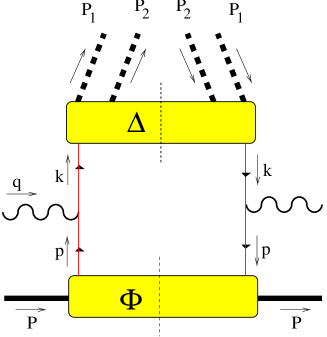
FIG. 1.: Quark diagram contributing in leading order to two-hadron inclusive DIS when both hadrons are in the same quark current jet. There is a similar diagram for anti-quarks.

II Single spin asymmetry for two hadron-inclusive lepton-nucleon DIS

In this Section, we discuss the general properties of two-hadron interference FF when the kinematics is specialized to semi-inclusive DIS, and for this process we work out the formula for a SSA that isolates the transversity at leading twist. However, we emphasize that under the assumption of factorization the soft parts of the process, i.e. the DF and the interference FF, are universal objects and, therefore, the results can be generalized to other hard processes, such as proton-proton scattering.

A Interference Fragmentation Functions in semi-inclusive DIS

At leading order, the hadron tensor for two unpolarized hadron-inclusive lepton-nucleon DIS reads [9]

$$2M\,{\cal W}^{\mu\nu} = \int{\rm d}p^{-}\,{\rm d}k^{+}\,{\rm d}^{2}{\vec{p}}_{\scriptscriptstyle T}\,{\rm d}^{2}{\vec{k}}_{\scriptscriptstyle T}\;\delta^{2}\!\left({\vec{p}}_{\scriptscriptstyle T}+{\vec{q}}_{\scriptscriptstyle T}-{\vec{k}}_{\scriptscriptstyle T}\right)\mbox{Tr}\big{[}\;\Phi(p;P,S)\;\gamma^{\mu}\;\Delta(k;P_{1},P_{2})\;\gamma^{\nu}\;\big{]}\Big{|}_{\begin{array}[]{c}p^{+}=xP^{+}\\ k^{-}=P_{h}^{-}/z\end{array}}$$ (6)

$${}+\left(\begin{array}[]{c}q\leftrightarrow-q\\ \mu\leftrightarrow\nu\end{array}\right)\;,$$

where $M$ is the target mass. The kinematics, also depicted in Fig. 1, represents a nucleon with momentum $P(P^{2}=M^{2})$ and a virtual hard photon with momentum $q$ that hits a quark carrying a fraction $p^{+}=xP^{+}$ of the parent hadron momentum. We describe a 4-vector $a$ as $\left[\;a^{-}\;,\;a^{+}\;,\;{\vec{a}}_{\scriptscriptstyle T}\;\right]$ in terms of its light-cone components $a^{\pm}=(a^{0}\pm a^{3})/\sqrt{2}$ and a transverse bidimensional vector ${\vec{a}}_{\scriptscriptstyle T}$. Because of momentum conservation in the hard vertex, the scattered quark has momentum $k=p+q$, and it fragments into two unpolarized hadrons, which carry a fraction $(P_{1}+P_{2})^{-}\equiv P_{h}^{-}=zk^{-}$ of the “parent quark” momentum, and the rest of the jet.

The quark-quark correlator $\Phi$ describes the nonperturbative processes that make the parton $p$ emerge from the spin-1/2 target, and it is symbolized by the lower shaded blob in Fig. 1. Using Lorentz invariance, hermiticity and parity invariance, the partly-integrated $\Phi$ can be parametrized at leading twist in terms of DF as

$$\Phi(x,{\vec{p}}_{\scriptscriptstyle T}) \equiv \left.\int{\rm d}p^{-}\;\Phi(p;P,S)\right|_{p^{+}=xP^{+}}\!\!\!\!=\frac{1}{2}\,\Biggl{\{}f_{1}\,{\kern 1.99997ptn\kern-4.49997pt/}_{+}+f_{1T}^{\perp}\,\epsilon_{\mu\nu\rho\sigma}\gamma^{\mu}\frac{n_{+}^{\nu}p_{\scriptscriptstyle T}^{\rho}S_{{\scriptscriptstyle T}}^{\sigma}}{M}-\left(\lambda\,g_{1L}+\frac{({\vec{p}}_{\scriptscriptstyle T}\cdot{\vec{S}}_{{\scriptscriptstyle T}})}{M}\,g_{1T}\right){\kern 1.99997ptn\kern-4.49997pt/}_{+}\gamma_{5}$$ (8)

$${}-h_{1T}\,i\sigma_{\mu\nu}\gamma_{5}S_{{\scriptscriptstyle T}}^{\mu}n_{+}^{\nu}-\left(\lambda\,h_{1L}^{\perp}+\frac{({\vec{p}}_{\scriptscriptstyle T}\cdot{\vec{S}}_{{\scriptscriptstyle T}})}{M}\,h_{1T}^{\perp}\right)\,\frac{i\sigma_{\mu\nu}\gamma_{5}p_{\scriptscriptstyle T}^{\mu}n_{+}^{\nu}}{M}+h_{1}^{\perp}\,\frac{\sigma_{\mu\nu}p_{\scriptscriptstyle T}^{\mu}n_{+}^{\nu}}{M}\Biggl{\}}\;,$$

where the DF depend on $x,{\vec{p}}_{\scriptscriptstyle T}$ and the polarization state of the target is fully specified by the light-cone helicity $\lambda=MS^{+}/P^{+}$ and the transverse component ${\vec{S}}_{\scriptscriptstyle T}$ of the target spin. Similarly, the correlator $\Delta$, symbolized by the upper shaded blob in Fig. 1, represents the fragmentation of the quark into the two detected hadrons and the rest of the current jet and can be parametrized as [9]

$$\Delta \equiv \left.\frac{1}{4z}\int{\rm d}k^{+}\;\Delta(k;P_{1},P_{2})\right|_{k^{-}=P_{h}^{-}/z}$$ (9)

$$= \frac{1}{4}\left\{D_{1}\,\kern 1.99997ptn\kern-4.49997pt/_{-}-G_{1}^{\perp}\,\frac{\epsilon_{\mu\nu\rho\sigma}\,\gamma^{\mu}\,n_{-}^{\nu}\,k_{\scriptscriptstyle T}^{\rho}\,R_{\scriptscriptstyle T}^{\sigma}}{M_{1}M_{2}}\,\gamma_{5}+H_{1}^{{<\kern-2.10002pt{\scriptscriptstyle)}}}\,\frac{\sigma_{\mu\nu}\,R_{\scriptscriptstyle T}^{\mu}\,n_{-}^{\nu}}{M_{1}M_{2}}+H_{1}^{\perp}\,\frac{\sigma_{\mu\nu}\,k_{\scriptscriptstyle T}^{\mu}\,n_{-}^{\nu}}{M_{1}M_{2}}\right\}\;,$$ (10)

where $n_{\pm}=\left[\;1\mp 1\;,\;1\pm 1\;,\;{\vec{0}}_{\scriptscriptstyle T}\;\right]/2$ are light-cone versors and $R\equiv(P_{1}-P_{2})/2$ is the relative momentum of the hadron pair.

For convenience, we will choose a frame where, besides $\vec{P}_{\scriptscriptstyle T}=0$, we have also $\vec{P}_{h{\scriptscriptstyle T}}=0$. By defining the light-cone momentum fraction $\xi=P_{1}^{-}/P_{h}^{-}$, we can parametrize the final-state momenta as

$$k = \left[\;\frac{P_{h}^{-}}{z}\;,\;z\frac{k^{2}+{\vec{k}}_{\scriptscriptstyle T}^{2}}{2P_{h}^{-}}\;,\;{\vec{k}}_{\scriptscriptstyle T}\;\right]\;,$$ (11)

$$P_{1} = \left[\;\xi\,P_{h}^{-}\;,\;\frac{M_{1}^{2}+{\vec{R}}_{\scriptscriptstyle T}^{2}}{2\,\xi\,P_{h}^{-}}\;,\;{\vec{R}}_{\scriptscriptstyle T}\;\right]\;,$$ (12)

$$P_{2} = \left[\;(1-\xi)\,P_{h}^{-}\;,\;\frac{M_{2}^{2}+{\vec{R}}_{\scriptscriptstyle T}^{2}}{2\,(1-\xi)\,P_{h}^{-}}\;,\;-{\vec{R}}_{\scriptscriptstyle T}\;\right]\;.$$ (13)

From the definition of the invariant mass of the hadron pair, i.e. $M_{h}^{2}\equiv P_{h}^{2}=2P_{h}^{+}P_{h}^{-}$, and the on-shell condition for the two hadrons themselves, $P_{1}^{2}=M_{1}^{2},P_{2}^{2}=M_{2}^{2}$, we deduce the relation

$${\vec{R}}_{\scriptscriptstyle T}^{2}=\xi\,(1-\xi)\,M_{h}^{2}-(1-\xi)\,M_{1}^{2}-\xi\,M_{2}^{2}$$ (14)

which in turn puts a constraint on the invariant mass from the positivity requirement ${\vec{R}}_{\scriptscriptstyle T}^{2}\geq 0$:

$$M_{h}^{2}\geq\frac{M_{1}^{2}}{\xi}+\frac{M_{2}^{2}}{1-\xi}\;.$$ (15)

After having given all the details of the kinematics, we can specify the actual dependence of the quark-quark correlator $\Delta$ and of the FF. From the frame choice $\vec{P}_{h{\scriptscriptstyle T}}=0$, the on-shell condition for both hadrons, Eq. (14), the constraint on $k^{-}$ and the integration over $k^{+}$ implied by the definition of $\Delta$ in Eq. (10), we deduce that the actual number of independent components of the three 4-vectors $k,P_{1},P_{2}$ is five (cf. [9]). They can conveniently be chosen as the fraction of quark momentum carried by the hadron pair, $z$, the subfraction in which this momentum is further shared inside the pair, $\xi$, and the “geometry” of the pair in the momentum space. Namely, the “opening” of the pair momenta, ${\vec{R}}_{\scriptscriptstyle T}^{2}$, the relative position of the jet axis and the hadron pair axis, ${\vec{k}}_{\scriptscriptstyle T}^{2}$, and the relative position of hadron pair plane and the plane formed by the jet axis and the hadron pair axis, ${\vec{k}}_{\scriptscriptstyle T}\cdot{\vec{R}}_{\scriptscriptstyle T}$ (see Fig. 2).

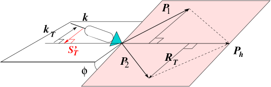
FIG. 2.: The kinematics for the final state where a quark fragments into two leading hadrons inside the same current jet.

Both DF and FF can be deduced from suitable projections of the corresponding quark-quark correlators. In particular, by defining

$$\Delta^{[\Gamma]}(z,\xi,{\vec{k}}_{\scriptscriptstyle T}^{2},{\vec{R}}_{\scriptscriptstyle T}^{2},{\vec{k}}_{\scriptscriptstyle T}\cdot{\vec{R}}_{\scriptscriptstyle T})\equiv\frac{1}{4z}\left.\int{\rm d}k^{+}\;\mbox{Tr}[\Gamma\,\Delta(k,P_{1},P_{2})]\right|_{k^{-}=P_{h}^{-}/z}\;,$$ (16)

we can deduce

$$\Delta^{[\gamma^{-}]} = D_{1}(z_{h},\xi,{\vec{k}}_{\scriptscriptstyle T}^{\,2},{\vec{R}}_{\scriptscriptstyle T}^{\,2},{\vec{k}}_{\scriptscriptstyle T}\cdot{\vec{R}}_{\scriptscriptstyle T})$$ (18)

$$\Delta^{[\gamma^{-}\gamma_{5}]} = \frac{\epsilon_{\scriptscriptstyle T}^{ij}\,R_{{\scriptscriptstyle T}i}\,k_{{\scriptscriptstyle T}j}}{M_{1}\,M_{2}}\;G_{1}^{\perp}(z_{h},\xi,{\vec{k}}_{\scriptscriptstyle T}^{\,2},{\vec{R}}_{\scriptscriptstyle T}^{\,2},{\vec{k}}_{\scriptscriptstyle T}\cdot{\vec{R}}_{\scriptscriptstyle T})$$ (19)

$$\Delta^{[i\sigma^{i-}\gamma_{5}]} = {\epsilon_{\scriptscriptstyle T}^{ij}R_{{\scriptscriptstyle T}j}\over M_{1}+M_{2}}\,H_{1}^{{<\kern-2.10002pt{\scriptscriptstyle)}}}(z_{h},\xi,{\vec{k}}_{\scriptscriptstyle T}^{\,2},{\vec{R}}_{\scriptscriptstyle T}^{\,2},{\vec{k}}_{\scriptscriptstyle T}\cdot{\vec{R}}_{\scriptscriptstyle T})+{\epsilon_{\scriptscriptstyle T}^{ij}k_{{\scriptscriptstyle T}j}\over M_{1}+M_{2}}\,H_{1}^{\perp}(z_{h},\xi,{\vec{k}}_{\scriptscriptstyle T}^{\,2},{\vec{R}}_{\scriptscriptstyle T}^{\,2},{\vec{k}}_{\scriptscriptstyle T}\cdot{\vec{R}}_{\scriptscriptstyle T})\;.$$ (20)

The leading-twist projections give a nice probabilistic interpretation of FF related to the Dirac operator $\Gamma$ used. Hence, $D_{1}$ is the probability for a unpolarized quark to fragment into the unpolarized hadron pair, $G_{1}^{\perp}$ is the probability difference for a longitudinally polarized quark with opposite chiralities to fragment into the pair, both $H_{1}^{\perp}$ and $H_{1}^{{<\kern-2.10002pt{\scriptscriptstyle)}}}$ give the same probability difference but for a transversely polarized fragmenting quark. A different interpretation for $H_{1}^{\perp}$ and $H_{1}^{{<\kern-2.10002pt{\scriptscriptstyle)}}}$ comes only from the possible origin for a non-vanishing probability difference, which is induced by the direction of $k_{\scriptscriptstyle T}$ and $R_{\scriptscriptstyle T}$, respectively. $G_{1}^{\perp},H_{1}^{\perp},H_{1}^{{<\kern-2.10002pt{\scriptscriptstyle)}}}$ are all naive T-odd and $H_{1}^{\perp},H_{1}^{{<\kern-2.10002pt{\scriptscriptstyle)}}}$ are further chiral-odd. $H_{1}^{{<\kern-2.10002pt{\scriptscriptstyle)}}}$ represents a genuine new effect with respect to the Collins one, because it relates the transverse polarization of the fragmenting quark to the orbital angular motion of the transverse component of the pair relative momentum ${\vec{R}}_{\scriptscriptstyle T}$ via the new angle $\phi$ defined by

$$\sin\phi=\frac{{\vec{S}}^{\prime}_{\scriptscriptstyle T}\cdot{\vec{P}}_{2}\times{\vec{P}}_{1}}{|{\vec{S}}^{\prime}_{\scriptscriptstyle T}||{\vec{P}}_{2}\times{\vec{P}}_{1}|}=\frac{{\vec{S}}^{\prime}_{\scriptscriptstyle T}\cdot{\vec{P}}_{h}\times{\vec{R}}}{|{\vec{S}}^{\prime}_{\scriptscriptstyle T}||{\vec{P}}_{h}\times{\vec{R}}|}\equiv\frac{{\vec{S}}^{\prime}_{\scriptscriptstyle T}\cdot{\vec{P}}_{h}\times{\vec{R}}_{\scriptscriptstyle T}}{|{\vec{S}}^{\prime}_{\scriptscriptstyle T}||{\vec{P}}_{h}\times{\vec{R}}_{\scriptscriptstyle T}|}=\cos\left(\phi_{S^{\prime}_{\scriptscriptstyle T}}-\frac{\pi}{2}-\phi_{R_{\scriptscriptstyle T}}\right)=\sin(\phi_{S_{\scriptscriptstyle T}}+\phi_{R_{\scriptscriptstyle T}})\;,$$ (21)

where we have used the condition ${\vec{P}}_{h{\scriptscriptstyle T}}=0$ and $\phi_{S_{\scriptscriptstyle T}}$ ($\phi_{S^{\prime}_{\scriptscriptstyle T}}$), $\phi_{R_{\scriptscriptstyle T}}$ are the azimuthal angles of the initial (final) quark transverse polarization and of ${\vec{R}}_{\scriptscriptstyle T}$ with respect to the scattering plane, respectively (see also Fig. 2).

B Isolating transversity from the SSA

Usually, the analysis of experimental observables is better accomplished in the frame where the target momentum $P$ and the momentum transfer $q$ are collinear and with no transverse components. Using a different notation, we have ${\vec{P}}_{\perp}={\vec{q}}_{\perp}=0$ and ${\vec{P}}_{h\perp}\neq 0$. An appropriate transverse Lorentz boost transforms this frame to the previous one where ${\vec{P}}_{\scriptscriptstyle T}={\vec{P}}_{h{\scriptscriptstyle T}}=0$ and ${\vec{q}}_{\scriptscriptstyle T}=-{\vec{P}}_{h\perp}/z$ [9]. However, the difference between the components of vectors in each frame is suppressed like ${\cal O}(1/Q)$. Since we are here considering expressions for the observables at leading twist only, this difference can be safely neglected.

By using Eq. (14), the complete cross section at leading twist for the two-hadron inclusive DIS of a unpolarized beam on a transversely polarized target, where two unpolarized hadrons are detected in the same quark current jet, is given by

$$\frac{{\rm d}\sigma}{{\rm d}\Omega\,{\rm d}x\,{\rm d}z\,{\rm d}\xi\,{\rm d}^{2}{\vec{P}}_{h\perp}\,{\rm d}M_{h}^{2}\,{\rm d}\phi_{R_{\perp}}}\,=\frac{\xi(1-\xi)}{2}\,\frac{{\rm d}\sigma}{{\rm d}\Omega\,{\rm d}x\,{\rm d}z\,{\rm d}\xi\,{\rm d}^{2}{\vec{P}}_{h\perp}\,{\rm d}^{2}{\vec{R}}_{\perp}}$$ (22)

$$\phantom{\frac{{\rm d}\sigma}{{\rm d}\Omega\,{\rm d}x\,{\rm d}z\,{\rm d}\xi\,{\rm d}^{2}{\vec{P}}_{h\perp}\,{\rm d}M_{h}^{2}\,{\rm d}\phi_{R_{\perp}}}\,}=\frac{{\rm d}\sigma_{OO}}{{\rm d}\Omega\,{\rm d}x\,{\rm d}z\,{\rm d}\xi\,{\rm d}^{2}{\vec{P}}_{h\perp}\,{\rm d}M_{h}^{2}\,{\rm d}\phi_{R_{\perp}}}\,+\,|{\vec{S}}_{\perp}|\,\frac{{\rm d}\sigma_{OT}}{{\rm d}\Omega\,{\rm d}x\,{\rm d}z\,{\rm d}\xi\,{\rm d}^{2}{\vec{P}}_{h\perp}\,{\rm d}M_{h}^{2}\,{\rm d}\phi_{R_{\perp}}}$$ (23)

$$= \frac{\alpha_{em}sx}{(2\pi)^{3}2Q^{4}}\,\Bigg{\{}{}A(y)\;{\cal F}\left[f_{1}\,D_{1}\right]$$ (27)

$${}+|{\vec{R}}_{\perp}|\;B(y)\;\sin(\phi_{h}+\phi_{R_{\perp}})\;{\cal F}\left[\,{\hat{g}}\!\cdot\!\vec{p}_{\scriptscriptstyle T}\,\frac{h_{1}^{\perp}\,H_{1}^{{<\kern-2.10002pt{\scriptscriptstyle)}}}}{M(M_{1}+M_{2})}\right]{}-|{\vec{R}}_{\perp}|\;B(y)\;\cos(\phi_{h}+\phi_{R_{\perp}})\;{\cal F}\left[\,{\hat{h}}\!\cdot\!\vec{p}_{\scriptscriptstyle T}\,\frac{h_{1}^{\perp}\,H_{1}^{{<\kern-2.10002pt{\scriptscriptstyle)}}}}{M(M_{1}+M_{2})}\right]$$

$${}-B(y)\;\cos(2\phi_{h})\;{\cal F}\left[\left(2\,{\hat{h}}\!\cdot\!\vec{p}_{\scriptscriptstyle T}\,\,{\hat{h}}\!\cdot\!\vec{k}_{\scriptscriptstyle T}\,-\,\vec{p}_{\scriptscriptstyle T}\!\cdot\!\vec{k}_{\scriptscriptstyle T}\,\right)\frac{h_{1}^{\perp}\,H_{1}^{\perp}}{M(M_{1}+M_{2})}\right]$$

$${}-B(y)\;\sin(2\phi_{h})\;{\cal F}\left[\left(\,{\hat{h}}\!\cdot\!\vec{p}_{\scriptscriptstyle T}\,\,{\hat{g}}\!\cdot\!\vec{k}_{\scriptscriptstyle T}\,+\,{\hat{h}}\!\cdot\!\vec{k}_{\scriptscriptstyle T}\,\,{\hat{g}}\!\cdot\!\vec{p}_{\scriptscriptstyle T}\,\right)\frac{h_{1}^{\perp}\,H_{1}^{\perp}}{M(M_{1}+M_{2})}\right]\Bigg{\}}$$

$$+ \frac{\alpha_{em}sx}{(2\pi)^{3}2Q^{4}}\,|{\vec{S}}_{\perp}|\,\Bigg{\{}A(y)\;\sin(\phi_{h}-\phi_{S_{\perp}})\;{\cal F}\left[\,{\hat{h}}\!\cdot\!\vec{p}_{\scriptscriptstyle T}\,\frac{f_{1T}^{\perp}\,D_{1}}{M}\right]\,+\,A(y)\;\cos(\phi_{h}-\phi_{S_{\perp}})\;{\cal F}\left[\,{\hat{g}}\!\cdot\!\vec{p}_{\scriptscriptstyle T}\,\frac{f_{1T}^{\perp}\,D_{1}}{M}\right]$$ (41)

$$\quad{}+B(y)\;\sin(\phi_{h}+\phi_{S_{\perp}}){\cal F}\left[\,{\hat{h}}\!\cdot\!\vec{k}_{\scriptscriptstyle T}\,\frac{h_{1}\,H_{1}^{\perp}}{M_{1}+M_{2}}\right]\,+\,B(y)\;\cos(\phi_{h}+\phi_{S_{\perp}}){\cal F}\left[\,{\hat{g}}\!\cdot\!\vec{k}_{\scriptscriptstyle T}\,\frac{h_{1}\,H_{1}^{\perp}}{M_{1}+M_{2}}\right]$$

$$\quad{}+|{\vec{R}}_{\perp}|\;B(y)\;\sin(\phi_{R_{\perp}}+\phi_{S_{\perp}})\;{\cal F}\left[\frac{h_{1}\,H_{1}^{{<\kern-2.10002pt{\scriptscriptstyle)}}}}{M_{1}+M_{2}}\right]$$

$$\quad{}-|{\vec{R}}_{\perp}|\;A(y)\;\cos(\phi_{h}-\phi_{S_{\perp}})\;\sin(\phi_{h}-\phi_{R_{\perp}})\;{\cal F}\left[\,{\hat{h}}\!\cdot\!\vec{k}_{\scriptscriptstyle T}\,\,{\hat{h}}\!\cdot\!\vec{p}_{\scriptscriptstyle T}\,\frac{g_{1T}\,G_{1}^{\perp}}{MM_{1}M_{2}}\right]$$

$$\quad{}+|{\vec{R}}_{\perp}|\;A(y)\;\sin(\phi_{h}-\phi_{S_{\perp}})\;\sin(\phi_{h}-\phi_{R_{\perp}})\;{\cal F}\left[\,{\hat{h}}\!\cdot\!\vec{k}_{\scriptscriptstyle T}\,\,{\hat{g}}\!\cdot\!\vec{p}_{\scriptscriptstyle T}\,\frac{g_{1T}\,G_{1}^{\perp}}{MM_{1}M_{2}}\right]$$

$$\quad{}-|{\vec{R}}_{\perp}|\;A(y)\;\cos(\phi_{h}-\phi_{S_{\perp}})\;\cos(\phi_{h}-\phi_{R_{\perp}})\;{\cal F}\left[\,{\hat{g}}\!\cdot\!\vec{k}_{\scriptscriptstyle T}\,\,{\hat{h}}\!\cdot\!\vec{p}_{\scriptscriptstyle T}\,\frac{g_{1T}\,G_{1}^{\perp}}{MM_{1}M_{2}}\right]$$

$$\quad{}+|{\vec{R}}_{\perp}|\;A(y)\;\sin(\phi_{h}-\phi_{S_{\perp}})\;\cos(\phi_{h}-\phi_{R_{\perp}})\;{\cal F}\left[\,{\hat{g}}\!\cdot\!\vec{k}_{\scriptscriptstyle T}\,\,{\hat{g}}\!\cdot\!\vec{p}_{\scriptscriptstyle T}\,\frac{g_{1T}\,G_{1}^{\perp}}{MM_{1}M_{2}}\right]$$

$$\quad{}+B(y)\;\cos(3\phi_{h}-\phi_{S_{\perp}})\;{\cal F}\left[\,{\hat{h}}\!\cdot\!\vec{k}_{\scriptscriptstyle T}\,\,{\hat{h}}\!\cdot\!\vec{p}_{\scriptscriptstyle T}\,\,{\hat{g}}\!\cdot\!\vec{p}_{\scriptscriptstyle T}\,\frac{h_{1T}^{\perp}\,H_{1}^{\perp}}{M^{2}(M_{1}+M_{2})}\right]$$

$$\quad{}+B(y)\;\sin(2\phi_{h})\,\cos(\phi_{h}-\phi_{S_{\perp}})\;{\cal F}\left[\,{\hat{h}}\!\cdot\!\vec{k}_{\scriptscriptstyle T}\,\left(\,{\hat{h}}\!\cdot\!\vec{p}_{\scriptscriptstyle T}\,\right)^{2}\frac{h_{1T}^{\perp}\,H_{1}^{\perp}}{M^{2}(M_{1}+M_{2})}\right]$$

$$\quad{}-B(y)\;\cos(2\phi_{h})\,\sin(\phi_{h}-\phi_{S_{\perp}})\;{\cal F}\left[\,{\hat{h}}\!\cdot\!\vec{k}_{\scriptscriptstyle T}\,\left(\,{\hat{g}}\!\cdot\!\vec{p}_{\scriptscriptstyle T}\,\right)^{2}\frac{h_{1T}^{\perp}\,H_{1}^{\perp}}{M^{2}(M_{1}+M_{2})}\right]$$

$$\quad{}-B(y)\;\sin(3\phi_{h}-\phi_{S_{\perp}})\;{\cal F}\left[\,{\hat{g}}\!\cdot\!\vec{k}_{\scriptscriptstyle T}\,\,{\hat{h}}\!\cdot\!\vec{p}_{\scriptscriptstyle T}\,\,{\hat{g}}\!\cdot\!\vec{p}_{\scriptscriptstyle T}\,\frac{h_{1T}^{\perp}\,H_{1}^{\perp}}{M^{2}(M_{1}+M_{2})}\right]$$

$$\quad{}+B(y)\;\cos(2\phi_{h})\,\cos(\phi_{h}-\phi_{S_{\perp}})\;{\cal F}\left[\,{\hat{g}}\!\cdot\!\vec{k}_{\scriptscriptstyle T}\,\left(\,{\hat{h}}\!\cdot\!\vec{p}_{\scriptscriptstyle T}\,\right)^{2}\frac{h_{1T}^{\perp}\,H_{1}^{\perp}}{M^{2}(M_{1}+M_{2})}\right]$$

$$\quad{}+B(y)\;\sin(2\phi_{h})\,\sin(\phi_{h}-\phi_{S_{\perp}})\;{\cal F}\left[\,{\hat{g}}\!\cdot\!\vec{k}_{\scriptscriptstyle T}\,\left(\,{\hat{g}}\!\cdot\!\vec{p}_{\scriptscriptstyle T}\,\right)^{2}\frac{h_{1T}^{\perp}\,H_{1}^{\perp}}{M^{2}(M_{1}+M_{2})}\right]$$

$$\quad{}+|{\vec{R}}_{\perp}|\;B(y)\;\sin(2\phi_{h}+\phi_{R_{\perp}}-\phi_{S_{\perp}}){\cal F}\left[\left(({\hat{h}}\!\cdot\!\vec{p}_{\scriptscriptstyle T})^{2}-({\hat{g}}\!\cdot\!\vec{p}_{\scriptscriptstyle T})^{2}+2\,{\hat{h}}\!\cdot\!\vec{p}_{\scriptscriptstyle T}\,\,{\hat{g}}\!\cdot\!\vec{p}_{\scriptscriptstyle T}\,\right)\frac{h_{1T}^{\perp}\,H_{1}^{{<\kern-2.10002pt{\scriptscriptstyle)}}}}{2M^{2}(M_{1}+M_{2})}\right]\Bigg{\}}\,,$$

where $\alpha_{em}$ is the fine structure constant, $s=Q^{2}/xy=-q^{2}/xy$ is the total energy in the center-of-mass system and

$$A(y)=\left(1-y+\frac{1}{2}y^{2}\right)\quad,\quad B(y)=(1-y)\quad,\quad C(y)=y(2-y)$$ (42)

with the lepton invariant $y=(P\cdot q)/(P\cdot l)\approx q^{-}/l^{-}$. The convolution of distribution and fragmentation functions is defined as

$${\cal F}\left[w({\vec{p}}_{\scriptscriptstyle T},{\vec{k}}_{\scriptscriptstyle T})\;f\,D\right]\equiv\;\sum_{a}e_{a}^{2}\;\int{\rm d}^{2}{\vec{p}}_{\scriptscriptstyle T}\;{\rm d}^{2}{\vec{k}}_{\scriptscriptstyle T}\;\delta^{2}({\vec{k}}_{\scriptscriptstyle T}-{\vec{p}}_{\scriptscriptstyle T}+\frac{{\vec{P}}_{h\perp}}{z})\;w({\vec{p}}_{\scriptscriptstyle T},{\vec{k}}_{\scriptscriptstyle T})\;f^{a}(x,{\vec{p}}_{\scriptscriptstyle T}^{\;2})\,D^{a}(z_{h},\xi,{\vec{k}}_{\scriptscriptstyle T}^{\,2},{\vec{R}}_{\scriptscriptstyle T}^{\,2},{\vec{k}}_{\scriptscriptstyle T}\cdot{\vec{R}}_{\scriptscriptstyle T})\;,$$ (43)

where $w({\vec{p}}_{\scriptscriptstyle T},{\vec{k}}_{\scriptscriptstyle T})$ is a weight function and the sum runs over all quark (and anti-quark) flavors, with $e_{a}$ the electric charges of the quarks. The versors appearing in the weight function $w$ are defined as ${\hat{h}}={\vec{P}}_{h\perp}/|{\vec{P}}_{h\perp}|$ and ${\hat{g}}^{i}=\epsilon_{\scriptscriptstyle T}^{ij}\,{\hat{h}}^{j}$ (with $\epsilon_{\scriptscriptstyle T}^{ij}\equiv\epsilon^{-+ij}$), respectively, and they represent the two independent directions in the $\perp$ plane perpendicular to ${\hat{z}}\parallel{\vec{q}}/|{\vec{q}}|$. All azimuthal angles $\phi_{S_{\perp}},\phi_{R_{\perp}}$ and $\phi_{h}$ (relative to ${\vec{P}}_{h\perp}$) lie in the $\perp$ plane and are measured with respect to the scattering plane (see Fig. 3). Eq. (41) corresponds to the sum of Eqs. (B1) and (B4) in Ref. [9], where, however, the expressions are simpler because they rely on the assumption of a symmetrical cylindrical distribution of hadron pairs around the jet axis, in order to have fragmentation functions depending on even powers of ${\vec{k}}_{\scriptscriptstyle T}$ only (this assumption would make all terms including the ${\hat{g}}$ versor disappear from Eq. (41); see also Ref. [15] for a comparison).

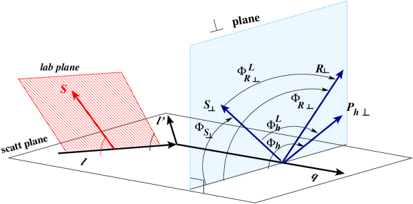
FIG. 3.: The definition of azimuthal angles, in the frame where $q_{\perp}=0$, with respect to the scattering plane and the laboratory plane, whose relative oriented angle is $\phi^{L}=-\phi_{S_{\perp}}$.

During experiments the scattering plane changes (different scales $Q$ imply different positions of the scattered beam). Therefore, it is better to define the laboratory frame as the plane formed by the beam and the direction of the target polarization. All azimuthal angles are conveniently reexpressed with respect to the laboratory frame as

$$\phi_{R_{\perp}} = \phi_{R_{\perp}}^{L}-\phi^{L}$$ (44)

$$\phi_{S_{\perp}} = -\phi^{L}$$ (45)

$$\phi_{h} = \phi_{h}^{L}-\phi^{L}\,,$$ (46)

where the superscript ^L indicates the new reference frame. The oriented angle between the scattering plane and the laboratory frame is $\phi^{L}$ (see Fig. 3). At leading order, the azimuthal angle of Eq. (21) becomes $\phi=\phi_{R_{\perp}}^{L}-2\phi^{L}$ in the new frame.

The new expression for the cross section is obtained by simply replacing Eq. (46) inside the angular dependence of Eq. (41). After replacement and apart from phase space coefficients, each term of the cross section will look like

$$d\sigma^{tw}\,\propto\,t(\phi_{R_{\perp}}^{L},\phi^{L},\phi_{h}^{L})\;{\cal F}\left[w\;\mbox{DF}\;\mbox{FF}\right]\,=\,t(\phi_{R_{\perp}}^{L},\phi^{L},\phi_{h}^{L})\;I(z,\xi,{\vec{R}}_{\scriptscriptstyle T}^{\,2})\,,$$ (47)

where $t$ is a trigonometric function, $w$ is the specific weight function for each combination of distribution and fragmentation functions (DF and FF, respectively), and $I$ is the result of the convolution integral. It is easy to verify that folding the cross section by

$$\frac{1}{2\pi}\int_{0}^{2\pi}{\rm d}\phi^{L}{\rm d}\phi_{R_{\perp}}^{L}\;\sin(\phi_{R_{\perp}}^{L}-2\phi^{L})\;\frac{{\rm d}\sigma}{{\rm d}\Omega\,{\rm d}x\,{\rm d}z\,{\rm d}\xi\,{\rm d}^{2}{\vec{P}}_{h\perp}\,{\rm d}M_{h}^{2}\,{\rm d}\phi_{R_{\perp}}}$$ (48)

makes only those $d\sigma^{tw}$ terms survive where $H_{1}^{{<\kern-2.10002pt{\scriptscriptstyle)}}}$ shows up in the convolution, i.e. for the following combinations

$$t=\cos(\phi_{h}^{L}+\phi_{R_{\perp}}^{L}-2\phi^{L}) \quad, \quad w={\hat{h}}\cdot{\vec{p}}_{\scriptscriptstyle T}\quad;$$ (50)

$$t=\sin(\phi_{h}^{L}+\phi_{R_{\perp}}^{L}-2\phi^{L}) \quad, \quad w={\hat{g}}\cdot{\vec{p}}_{\scriptscriptstyle T}\quad;$$ (51)

$$t=\sin(\phi_{R_{\perp}}^{L}-2\phi^{L}) \quad, \quad w=1\quad;$$ (52)

$$t=\sin(2\phi_{h}^{L}+\phi_{R_{\perp}}^{L}-2\phi^{L}) \quad, \quad w=\left(({\hat{h}}\cdot{\vec{p}}_{\scriptscriptstyle T})^{2}-({\hat{g}}\cdot{\vec{p}}_{\scriptscriptstyle T})^{2}+2\,{\hat{h}}\cdot{\vec{p}}_{\scriptscriptstyle T}\,{\hat{g}}\cdot{\vec{p}}_{\scriptscriptstyle T}\right)\,.$$ (53)

Similarly, it is straightforward to proof that integrating these surviving terms upon ${\rm d}^{2}{\vec{P}}_{h\perp}$, and performing the integrals in the convolution ${\cal F}[w\;\mbox{DF}\;\mbox{FF}]$, makes only the combination (52) to survive presenting the transversity in a factorized form. In fact, by integrating also upon ${\rm d}\xi$ we finally have

$$\frac{<{\rm d}\sigma_{OT}>}{{\rm d}y\,{\rm d}x\,{\rm d}z\,{\rm d}M_{h}^{2}} \equiv \frac{1}{2\pi}\,\int_{0}^{2\pi}{\rm d}\phi^{L}\,{\rm d}\phi_{R_{\perp}}^{L}\int{\rm d}^{2}{\vec{P}}_{h\perp}\;\int{\rm d}\xi\;\sin(\phi_{R_{\perp}}^{L}-2\phi^{L})\;\frac{{\rm d}\sigma}{{\rm d}\Omega\,{\rm d}x\,{\rm d}z\,{\rm d}\xi\,{\rm d}M_{h}^{2}\,{\rm d}\phi_{R_{\perp}}^{L}\,{\rm d}^{2}{\vec{P}}_{h\perp}}$$ (54)

$$= \frac{\pi\alpha_{em}^{2}sx}{(2\pi)^{3}Q^{4}}\;\frac{B(y)\,|{\vec{S}}_{\perp}|}{2(M_{1}+M_{2})}\;\sum_{a}e_{a}^{2}\;\int{\rm d}^{2}{\vec{p}}_{\scriptscriptstyle T}\;h_{1}^{a}(x,{\vec{p}}_{\scriptscriptstyle T}^{\;2})$$ (56)

$$\times\int{\rm d}\xi\;|{\vec{R}}_{\perp}|\int_{0}^{2\pi}{\rm d}\phi_{R_{\perp}}^{L}\int{\rm d}^{2}{\vec{k}}_{\scriptscriptstyle T}\;H_{1}^{{<\kern-2.10002pt{\scriptscriptstyle)}}\,a}(z,\xi,M_{h}^{2},{\vec{k}}_{\scriptscriptstyle T}^{\;2},{\vec{k}}_{\scriptscriptstyle T}\cdot{\vec{R}}_{\scriptscriptstyle T})$$

$$= \frac{\pi\alpha_{em}^{2}s}{(2\pi)^{3}Q^{4}}\;\frac{B(y)\,|{\vec{S}}_{\perp}|}{2(M_{1}+M_{2})}\;\sum_{a}e_{a}^{2}\;x\;h_{1}^{a}(x)\;H_{1\,(R)}^{{<\kern-2.10002pt{\scriptscriptstyle)}}\,a}(z,M_{h}^{2})\,,$$ (57)

where, for sake of simplicity, the same notations are kept for DF and FF before and after integration, distinguished by the explicit arguments only; the subscript _(R) reminds of the additional weighting factor $|\vec{R}_{\perp}|$. Analogously,

$$\frac{<{\rm d}\sigma_{OO}>}{{\rm d}y\,{\rm d}x\,{\rm d}z\,{\rm d}M_{h}^{2}} \equiv \frac{1}{2\pi}\,\int_{0}^{2\pi}{\rm d}\phi^{L}\,{\rm d}\phi_{R_{\perp}}^{L}\int{\rm d}^{2}{\vec{P}}_{h\perp}\;\int{\rm d}\xi\;\frac{{\rm d}\sigma}{{\rm d}\Omega\,{\rm d}x\,{\rm d}z\,{\rm d}\xi\,{\rm d}M_{h}^{2}\,{\rm d}\phi_{R_{\perp}}^{L}\,{\rm d}^{2}{\vec{P}}_{h\perp}}$$ (58)

$$= \frac{\pi\alpha_{em}^{2}sx}{(2\pi)^{3}Q^{4}}\,A(y)\,\sum_{a}e_{a}^{2}\;\int{\rm d}^{2}{\vec{p}}_{\scriptscriptstyle T}\;f_{1}^{a}(x,{\vec{p}}_{\scriptscriptstyle T}^{\;2})$$ (60)

$$\times\int{\rm d}\xi\int_{0}^{2\pi}{\rm d}\phi_{R_{\perp}}^{L}\int{\rm d}^{2}{\vec{k}}_{\scriptscriptstyle T}\;D_{1}^{a}(z,\xi,M_{h}^{2},{\vec{k}}_{\scriptscriptstyle T}^{\;2},{\vec{k}}_{\scriptscriptstyle T}\cdot{\vec{R}}_{\scriptscriptstyle T})$$

$$= \frac{\pi\alpha_{em}^{2}s}{(2\pi)^{3}Q^{4}}\,A(y)\,\sum_{a}e_{a}^{2}\;x\;f_{1}^{a}(x)\;D_{1}^{a}(z,M_{h}^{2})\,,$$ (61)

from which we can build the single spin asymmetry

$$A^{\sin\phi}(y,x,z,M_{h}^{2}) \equiv \frac{<{\rm d}\sigma_{OT}>}{{\rm d}y\,{\rm d}x\,{\rm d}z\,{\rm d}M_{h}^{2}}\,\left[\frac{<{\rm d}\sigma_{OO}>}{{\rm d}y\,{\rm d}x\,{\rm d}z\,{\rm d}M_{h}^{2}}\right]^{-1}$$ (62)

$$= \frac{B(y)}{A(y)}\;\frac{|{\vec{S}}_{\perp}|}{2(M_{1}+M_{2})}\;\frac{\sum_{a}e_{a}^{2}\;x\,h_{1}^{a}(x)\,H_{1\,(R)}^{{<\kern-2.10002pt{\scriptscriptstyle)}}\,a}(z,M_{h}^{2})}{\sum_{a}e_{a}^{2}\;x\,f_{1}^{a}(x)\,D_{1}^{a}(z,M_{h}^{2})}\,.$$ (63)

III Spectator model for $\pi^{+}\pi^{-}$ fragmentation

In the field theoretical description of hard processes, the FF represent the soft processes that connect the hard quark to the detected hadrons via fragmentation, i.e. they are hadronic matrix elements of nonlocal operators built from quark (and gluon) fields [16]. For a quark fragmenting into two hadrons inside the same current jet, the appropriate quark-quark correlator (in the light-cone gauge) reads [12, 11]

$$\Delta_{ij}(k,P_{1},P_{2})=\kern 1.99997pt{\textstyle\sum}\kern-11.00008pt\int_{X}\;\int\frac{{\rm d}^{4\!}\zeta}{(2\pi)^{4}}\;e^{ik\cdot\zeta}\;\langle 0|\psi_{i}(\zeta)|P_{1},P_{2},X\rangle\langle X,P_{2},P_{1}|\overline{\psi}_{j}(0)|0\rangle\,,$$ (64)

where the sum runs over all the possible intermediate states containing the hadron pair.

FIG. 4.: The diagrams considered for the quark fragmentation into $\pi^{+}\pi^{-}$ at leading twist and leading order in $\alpha_{s}$ in the context of the spectator model.

The basic idea of the spectator model is to make a specific ansatz for this spectral decomposition by replacing the sum with an effective spectator state with a definite mass and quantum numbers [17, 18, 14]. By specializing the model to the case of $\pi^{+}\pi^{-}$ fragmentation with $P_{1}=P_{\pi^{+}}$ and $P_{2}=P_{\pi^{-}}$, the spectator has the quantum numbers of an on-shell valence quark with a constituent mass $m_{q}=340$ MeV. Consequently, the quark-quark correlator (64) simplifies to

$$\Delta_{ij}(k,P_{\pi^{+}},P_{\pi^{-}}) \approx \frac{\theta\!\left((k-P_{h})^{+}\right)}{(2\pi)^{3}}\;\delta\left((k-P_{h})^{2}-m_{q}^{2}\right)\;\langle 0|\psi_{i}(0)|P_{\pi^{+}},P_{\pi^{-}},q\rangle\langle q,P_{\pi^{-}},P_{\pi^{+}}|\overline{\psi}_{j}(0)|0\rangle$$ (65)

$$\equiv \widetilde{\Delta}_{ij}(k,P_{\pi^{+}},P_{\pi^{-}})\;\delta(\tau_{h}-\sigma_{h}+M_{h}^{2}-m_{q}^{2})\;,$$ (66)

where $\tau_{h}=k^{2}$ and $\sigma_{h}=2k\cdot P_{h}$. When inserting Eq. (66) into Eq. (16), the projections drastically simplify to

$$\Delta^{[\Gamma]}(z_{h},\xi,{\vec{k}}_{\scriptscriptstyle T}^{\,2},\vec{R}_{\scriptscriptstyle T}^{\,2},{\vec{k}}_{\scriptscriptstyle T}\cdot{\vec{R}}_{\scriptscriptstyle T})=\left.\frac{\mbox{Tr}[\Gamma\,\widetilde{\Delta}]}{8(1-z)P_{h}^{-}}\right|_{\tau_{h}=\tau_{h}(z,{\vec{k}}_{\scriptscriptstyle T}^{\,2})}\;,$$ (67)

with

$$\tau_{h}(z,{\vec{k}}_{\scriptscriptstyle T}^{\,2})=\frac{z}{1-z}{\vec{k}}_{\scriptscriptstyle T}^{\,2}+\frac{m_{q}^{2}}{1-z}+\frac{M_{h}^{2}}{z}\;.$$ (68)

We will consider the $\pi^{+}\pi^{-}$ system with an invariant mass $M_{h}$ close to the $\rho$ resonance, specifically $m_{\rho}-\Gamma_{\rho}/2\leq M_{h}\leq m_{\rho}+\Gamma_{\rho}/2$, where $\Gamma_{\rho}$ is the width of the $\rho$ resonance. Hence, the most appropriate and simplest diagrams that can replace the quark decay of Fig. 1 at leading twist, and leading order in $\alpha_{s}$, are represented in Fig. 4: the $\pi^{+}\pi^{-}$ can be produced from the $\rho$ decay or directly via a quark exchange in the $t$-channel (the background diagram); the quantum interference of the two processes generates the naive T-odd FF described in Sec. II A. A suitable selection of “Feynman” rules for the vertices and propagators of the diagrams in Fig. 4 allows for the analytic calculation of the matrix elements defining $\widetilde{\Delta}$ in Eq. (66) and, consequently, of the projections $\Delta^{[\Gamma]}$ defining the FF.

A Propagators

The propagators involved in the diagrams of Fig. 4 are:

• quark with momentum $\kappa$

  

  $$\left(\frac{i}{\kern 1.99997pt\kappa\kern-4.49997pt/-m_{q}}\right)_{ij}$$

  The propagator occurs with $\kappa^{2}=\tau_{h}\equiv k^{2}$ or $\kappa^{2}=(k-P_{\pi^{+}})^{2}$. In both cases, the off-shell condition $k^{2}\neq m_{q}^{2}$ is guaranteed by Eq. (68).

• $\rho$ with momentum $P_{h}$

  

  $$\frac{i}{P_{h}^{2}-m_{\rho}^{2}+im_{\rho}\Gamma_{\rho}}\left(-g^{\mu\nu}+\frac{P_{h}^{\mu}\,P_{h}^{\nu}}{P_{h}^{2}}\right)$$

  where $\Gamma_{\rho}=\displaystyle{\frac{f^{2}_{\rho\pi\pi}}{4\pi}\frac{m_{\rho}}{12}\left(1-\frac{4m_{\pi}^{2}}{m_{\rho}^{2}}\right)^{\frac{3}{2}}}$ [19].

B Vertices

In analogy with previous works on spectator models [18, 14], we choose the vertex form factors to depend on one invariant only, generally denoted $\kappa^{2}$, that represents the virtuality of the external entering quark line. Therefore, we can have $\kappa^{2}=\tau_{h}\equiv k^{2}$ or $\kappa^{2}=(k-P_{\pi^{+}})^{2}$. The power laws are such that the asymptotic behaviour is in agreement with the expectations based on dimensional counting rules. Finally, the normalization coefficients have dimensions such that $\int{\rm d}^{2}{\vec{k}}_{\scriptscriptstyle T}\int{\rm d}^{2}{\vec{R}}_{\scriptscriptstyle T}\,D_{1}(z,\xi,{\vec{k}}_{\scriptscriptstyle T}^{2},{\vec{R}}_{\scriptscriptstyle T}^{2},{\vec{k}}_{\scriptscriptstyle T}\cdot{\vec{R}}_{\scriptscriptstyle T})$ is a pure number to be interpreted as the probability for the hadron pair to carry a $z$ fraction of the valence quark momentum and to share it in $\xi$ and $1-\xi$ parts.

• $\rho\pi\pi$ vertex

  

  $$\Upsilon^{\rho\pi\pi,\mu}=f_{\rho\pi\pi}R^{\mu}$$

  where $\displaystyle{\frac{f_{\rho\pi\pi}^{2}}{4\pi}}=2.84\pm 0.50$ [19].

• $q\rho q$ vertex

  

  $$\Upsilon^{q\rho q,\mu}_{ij} = \frac{f_{q\rho q}(\kappa^{2})}{\sqrt{2}}\;[\gamma^{\mu}]_{ij}$$

  $$= \frac{N_{q\rho}}{\sqrt{2}}\;\frac{1}{|\kappa^{2}-\Lambda_{\rho}^{2}|^{\alpha}}\;[\gamma^{\mu}]_{ij}$$

  where $\Lambda_{\rho}$ excludes large virtualities of the quark. The power $\alpha$ is determined consistently with the quark counting rule that determines the asymptotic behaviour of the FF at large $z$ [19], i.e.

  $$(1-z)^{2\alpha-1}=(1-z)^{-3+2r+2|\lambda|}\,,$$ (69)

  where $r$ is the number of constituent quarks in the considered hadron, and $\lambda$ is the difference between the quark and the hadron helicities. Thus, here we have $\alpha=3/2$. The normalization $N_{q\rho}$ is such that the sum rule

  $$\int_{0}^{1}{\rm d}z\;z\,D_{1}(z)\leq 1$$ (70)

  is satisfied. In fact, in the infinite momentum frame the integral in Eq. (70) represents the total fraction $z$ of the quark energy taken by all hadron pairs of the type under consideration. Since in this frame low-energy mass effects can be neglected, we estimate that charged pion pairs with an invariant mass inside the $\rho$ resonance width represent $\sim 50\%$ of the total pions detected in the calorimeter, which in turn can be considered $\sim 80\%$ of all particles detected. Neglecting mass effects, we may assume that the fraction of quark energy taken by charged pions, relative to the energy taken by other hadrons, follows their relative numbers. Therefore, we chose two values, $N_{q\rho}=0.9$ GeV³ and $1.6$ GeV³, which correspond to rather extreme scenarios where the integral Eq. (70) amounts to 0.14 and 0.48, respectively.

• $q\pi q$ vertex

  

  $$\Upsilon^{q\pi q}_{ij} = \frac{f_{q\pi q}(\kappa^{2})}{\sqrt{2}}\;[\gamma_{5}]_{ij}$$

  $$= \frac{N_{q\pi}}{\sqrt{2}}\,\frac{1}{|\kappa^{2}-\Lambda_{\pi}^{2}|^{\alpha}}\;[\gamma_{5}]_{ij}$$

  where $\Lambda_{\pi}$ excludes large virtualities of the quark, as well. From quark counting rules, still $\alpha=3/2$. The normalization $N_{q\pi}$ can be deduced from $N_{q\rho}$ by generalizing the Goldberger-Treiman relation to the $\rho$-quark coupling [20]:

  $$\frac{g_{\pi qq}^{2}}{4\pi} = \left(\frac{g_{q}^{A}}{g_{N}^{A}}\right)^{2}\left(\frac{m_{q}}{m_{N}}\right)^{2}\frac{g_{\pi NN}^{2}}{4\pi}=\left(\frac{3}{5}\right)^{2}\left(\frac{340}{939}\right)^{2}14.2=0.67$$ (71)

  $$\frac{(g_{\rho qq}^{V}+g_{\rho qq}^{T})^{2}}{4\pi} = \left(\frac{g_{q}^{A}}{g_{N}^{A}}\right)^{2}\left(\frac{m_{q}}{m_{N}}\right)^{2}\frac{(g_{\rho NN}^{V}+g_{\rho NN}^{T})^{2}}{4\pi}=\left(\frac{3}{5}\right)^{2}\left(\frac{340}{939}\right)^{2}27.755=1.31\,,$$ (72)

  where $g^{A}_{N},m_{N}$ are the nucleon axial coupling constants and mass, respectively, as well as $g^{A}_{q},m_{q}$ the quark ones. The $\pi NN$ coupling is $g_{\pi NN}^{2}/4\pi=14.2$; the vector $\rho NN$ coupling is $(g_{\rho NN}^{V})^{2}/4\pi=0.55$ and its ratio to the tensor coupling is $g_{\rho NN}^{T}/g_{\rho NN}^{V}=6.105$ [21]. From the above relations, we deduce

  $$\frac{g_{\pi qq}}{(g_{\rho qq}^{V}+g_{\rho qq}^{T})}\equiv\frac{N_{q\pi}}{N_{q\rho}}=0.715\,.$$ (73)

As a final comment, we have explicitly checked that with the above rules the background diagram leads to a cross section that qualitatively shows the same $s$ dependence of experimental data for $\pi\pi$ production in the relative $L=0$ channel when $s$ is inside the $\rho$ resonance width, in any case below the first dip corresponding to the resonance $f_{0}(980)$ [22]. If we reasonably assume that the resonant diagram exhausts almost all of the $\pi\pi$ production in the relative $L=1$ channel and we also assume that in the given energy interval the $L=0,1$ channels approximate the whole strength for $\pi\pi$ production, we can safely state that the diagrams of Fig. 4 give a satisfactory reproduction of the $\pi\pi$ cross section, with invariant mass in the given interval, without invoking any scalar $\sigma$ resonance (cf. [11, 13]).

C Interference FF

With the above rules applied to the diagrams of Fig. 4, we can calculate all the matrix elements of Eq. (66) and, consequently, all the projections (67) leading to the FF. The naive T-odd $G_{1}^{\perp},H_{1}^{\perp},H_{1}^{{<\kern-2.10002pt{\scriptscriptstyle)}}}$ receive contributions from the interference diagrams only. In particular, they result proportional to the imaginary part of the $\rho$ propagator ($\sim m_{\rho}\Gamma_{\rho}$), while the real part ($\sim M_{h}^{2}-m_{\rho}^{2}$) contributes to $D_{1}$. Therefore, contrary to the findings of Ref. [13], a complex amplitude with a resonant behaviour is needed here to produce nonvanishing interference FF. For a $u$ quark fragmenting into $\pi^{+}\pi^{-}$, we have at leading twist

$$D_{1}^{u\rightarrow\pi^{+}\pi^{-}}(z,\xi,M_{h}^{2},k_{\scriptscriptstyle T}^{2},{\vec{k}}_{\scriptscriptstyle T}\cdot{\vec{R}}_{\scriptscriptstyle T})\;=\;\frac{N_{q\rho}^{2}\,f_{\rho\pi\pi}^{2}\,z^{2}\,(1-z)^{2}}{4(2\pi)^{3}\,[(M_{h}^{2}-m_{\rho}^{2})^{2}+m_{\rho}^{2}\,\Gamma_{\rho}^{2}]\,a^{2}\,|a+b|^{3}}$$ (80)

$$\qquad\qquad\times\Bigg{\{}\frac{c}{4}[\,c-za(2\xi-1)]+z^{2}(1-z)\left(\frac{M_{h}^{2}}{4}-m_{\pi}^{2}\right)[\,a-(1-z)M_{h}^{2}\,]\Bigg{\}}$$

$${}+\frac{N_{q\pi}^{4}\,z^{7}\,(1-z)^{7}}{8(2\pi)^{3}\,a^{2}\,d^{2}\,|d+{\tilde{b}}|^{3}\,|a+{\tilde{b}}|^{3}}$$

$$\qquad\times\Bigg{\{}-az\,[z\xi(1-z)+(1-\xi)d]-z(1-z)m_{\pi}^{2}\,\frac{a-c-z(1-z)M_{h}^{2}}{2}\,+\,d\,\frac{a-c+z(1-z)M_{h}^{2}}{2}\Bigg{\}}$$

$${}+\frac{\sqrt{2}\,(M_{h}^{2}-m_{\rho}^{2})\,z^{\frac{9}{2}}\,(1-z)^{\frac{9}{2}}\,N_{q\pi}^{2}\,N_{q\rho}\,f_{\rho\pi\pi}}{8(2\pi)^{3}[(M_{h}^{2}-m_{\rho}^{2})^{2}+m_{\rho}^{2}\,\Gamma_{\rho}^{2}]\,a^{2}\,d\,|a+b|^{\frac{3}{2}}\,|a+{\tilde{b}}|^{\frac{3}{2}}\,|d+{\tilde{b}}|^{\frac{3}{2}}}$$

$$\qquad\times\Bigg{\{}az(1-z)\left(2m_{\pi}^{2}-\frac{M_{h}^{2}}{2}\right)+\frac{a(1-2z\xi)+c+z(1-z)M_{h}^{2}}{4}\,[\,d+z(1-z)(M_{h}^{2}-5m_{\pi}^{2})]$$

$$\qquad\qquad{}+\,\frac{a\,[2z(1-\xi)-1]+c-z(1-z)M_{h}^{2}}{4}\,[\,3d-a+z(1-z)m_{\pi}^{2}\,]\Bigg{\}}$$

$$H_{1}^{{<\kern-2.10002pt{\scriptscriptstyle)}}\,u\rightarrow\pi^{+}\pi^{-}}(z,\xi,M_{h}^{2},k_{\scriptscriptstyle T}^{2},{\vec{k}}_{\scriptscriptstyle T}\cdot{\vec{R}}_{\scriptscriptstyle T})=$$ (82)

$${}-\,\frac{m_{\rho}\,\Gamma_{\rho}\,m_{\pi}\,m_{q}\,z^{\frac{13}{2}}\,(1-z)^{\frac{11}{2}}\,N_{q\pi}^{2}\,N_{q\rho}\,f_{\rho\pi\pi}}{2\sqrt{2}(2\pi)^{3}[(M_{h}^{2}-m_{\rho}^{2})^{2}+m_{\rho}^{2}\Gamma_{\rho}^{2}]\,a\,d\,|a+b|^{\frac{3}{2}}\,|a+{\tilde{b}}|^{\frac{3}{2}}\,|d+z(1-z)(m_{q}^{2}-\Lambda_{\pi}^{2})|^{\frac{3}{2}}}$$

$$H_{1}^{\perp\,u\rightarrow\pi^{+}\pi^{-}}(z,\xi,M_{h}^{2},k_{\scriptscriptstyle T}^{2},{\vec{k}}_{\scriptscriptstyle T}\cdot{\vec{R}}_{\scriptscriptstyle T})=0$$ (84)

$$G_{1}^{\perp\,u\rightarrow\pi^{+}\pi^{-}}(z,\xi,M_{h}^{2},k_{\scriptscriptstyle T}^{2},{\vec{k}}_{\scriptscriptstyle T}\cdot{\vec{R}}_{\scriptscriptstyle T})=-\frac{m_{\pi}}{2m_{q}}\,H_{1}^{{<\kern-2.10002pt{\scriptscriptstyle)}}\,u\rightarrow\pi^{+}\pi^{-}}(z,\xi,M_{h}^{2},k_{\scriptscriptstyle T}^{2},{\vec{k}}_{\scriptscriptstyle T}\cdot{\vec{R}}_{\scriptscriptstyle T})\,,$$

where

$$a = z^{2}(k_{\scriptscriptstyle T}^{2}+m_{q}^{2})+(1-z)M_{h}^{2}\quad,\quad b=z(1-z)(m_{q}^{2}-\Lambda_{\rho}^{2})\quad,\quad{\tilde{b}}=z(1-z)(m_{q}^{2}-\Lambda_{\pi}^{2})$$ (85)

$$c = (2\xi-1)[z^{2}(k_{\scriptscriptstyle T}^{2}+m_{q}^{2})-(1-z)^{2}M_{h}^{2}]-4z(1-z){\vec{k}}_{\scriptscriptstyle T}\cdot{\vec{R}}_{\scriptscriptstyle T}$$ (86)

$$d = z^{2}(1-\xi)(k_{\scriptscriptstyle T}^{2}+m_{q}^{2})+\xi(1-z)^{2}M_{h}^{2}+z(1-z)(m_{\pi}^{2}+2{\vec{k}}_{\scriptscriptstyle T}\cdot{\vec{R}}_{\scriptscriptstyle T})\,.$$ (87)

The simplifications induced by the spectator model reduce the number of independent FF, Eq. (84), and make $H_{1}^{\perp}$ vanish, i.e. the analogue of the Collins effect in this context turns out to be a higher-order effect. The structure induced by the model is simply not rich enough to produce a non-vanishing $H_{1}^{\perp}$. Moreover, the FF do not depend on the flavor of the fragmenting valence quark, provided that the charges of the final detected pions are selected according to the diagrams of Fig. 4. Hence, the FF are the same for $u\rightarrow\pi^{+}\pi^{-}$ and for $d\rightarrow\pi^{-}\pi^{+}$, where the final state differs only by the interchange of the two pions, i.e. by leaving everything unaltered but ${\vec{R}}_{\scriptscriptstyle T}\rightarrow-{\vec{R}}_{\scriptscriptstyle T}$ and $\xi\rightarrow(1-\xi)$:

$$D_{1}^{\,u\rightarrow\pi^{+}\pi^{-}}(z,\xi,M_{h}^{2},k_{\scriptscriptstyle T}^{2},{\vec{k}}_{\scriptscriptstyle T}\cdot{\vec{R}}_{\scriptscriptstyle T}) = D_{1}^{\,d\rightarrow\pi^{-}\pi^{+}}(z,\xi,M_{h}^{2},k_{\scriptscriptstyle T}^{2},{\vec{k}}_{\scriptscriptstyle T}\cdot{\vec{R}}_{\scriptscriptstyle T})$$ (88)

$$= D_{1}^{\,d\rightarrow\pi^{+}\pi^{-}}(z,(1-\xi),M_{h}^{2},k_{\scriptscriptstyle T}^{2},{\vec{k}}_{\scriptscriptstyle T}\cdot(-{\vec{R}}_{\scriptscriptstyle T}))$$ (89)

$$H_{1}^{{<\kern-2.10002pt{\scriptscriptstyle)}}\,u\rightarrow\pi^{+}\pi^{-}}(z,\xi,M_{h}^{2},k_{\scriptscriptstyle T}^{2},{\vec{k}}_{\scriptscriptstyle T}\cdot{\vec{R}}_{\scriptscriptstyle T}) = H_{1}^{{<\kern-2.10002pt{\scriptscriptstyle)}}\,d\rightarrow\pi^{-}\pi^{+}}(z,\xi,M_{h}^{2},k_{\scriptscriptstyle T}^{2},{\vec{k}}_{\scriptscriptstyle T}\cdot{\vec{R}}_{\scriptscriptstyle T})$$ (90)

$$= H_{1}^{{<\kern-2.10002pt{\scriptscriptstyle)}}\,d\rightarrow\pi^{+}\pi^{-}}(z,(1-\xi),M_{h}^{2},k_{\scriptscriptstyle T}^{2},{\vec{k}}_{\scriptscriptstyle T}\cdot(-{\vec{R}}_{\scriptscriptstyle T}))\,.$$ (91)

When integrating the FF over ${\rm d}^{2}{\vec{k}}_{\scriptscriptstyle T}$ and ${\rm d}\xi$, the dependence on the direction of ${\vec{R}}_{\scriptscriptstyle T}$ is lost

$$D_{1}^{\,u\rightarrow\pi^{+}\pi^{-}}(z,M_{h}^{2}) \equiv \int_{0}^{1}{\rm d}\xi\int{\rm d}^{2}{\vec{k}}_{\scriptscriptstyle T}\;D_{1}^{\,u\rightarrow\pi^{+}\pi^{-}}(z,\xi,M_{h}^{2},k_{\scriptscriptstyle T}^{2},{\vec{k}}_{\scriptscriptstyle T}\cdot{\vec{R}}_{\scriptscriptstyle T})$$ (92)

$$= \int_{0}^{1}{\rm d}\xi\int{\rm d}^{2}{\vec{k}}_{\scriptscriptstyle T}\;D_{1}^{\,d\rightarrow\pi^{+}\pi^{-}}(z,(1-\xi),M_{h}^{2},k_{\scriptscriptstyle T}^{2},{\vec{k}}_{\scriptscriptstyle T}\cdot(-{\vec{R}}_{\scriptscriptstyle T}))$$ (93)

$$= \int_{0}^{1}{\rm d}\xi\int{\rm d}^{2}{\vec{k}}_{\scriptscriptstyle T}\;D_{1}^{\,d\rightarrow\pi^{+}\pi^{-}}(z,\xi,M_{h}^{2},k_{\scriptscriptstyle T}^{2},{\vec{k}}_{\scriptscriptstyle T}\cdot(-{\vec{R}}_{\scriptscriptstyle T}))$$ (94)

$$\equiv D_{1}^{\,d\rightarrow\pi^{+}\pi^{-}}(z,M_{h}^{2})\,,$$ (95)

and similarly for $H_{1}^{{<\kern-2.10002pt{\scriptscriptstyle)}}}$. Therefore, we can conclude that the integrated FF do not depend in general on the flavor of the fragmenting quark.

Consequently, the SSA of Eq. (63) simplifies to

$$A^{\sin\phi}(y,x,z,M_{h}^{2})=\frac{B(y)}{A(y)}\;\frac{|{\vec{S}}_{\perp}|}{4m_{\pi}}\;\frac{\left[\displaystyle{\frac{8}{9}x\,h_{1}^{u}(x)+\frac{1}{9}x\,h_{1}^{d}(x)}\right]\;H_{1\,(R)}^{{<\kern-2.10002pt{\scriptscriptstyle)}}\,u}(z,M_{h}^{2})}{\left[\displaystyle{\frac{8}{9}x\,f_{1}^{u}(x)+\frac{1}{9}x\,f_{1}^{d}(x)}\right]\;D_{1}^{u}(z,M_{h}^{2})}\,.$$ (96)

In the following, we will discuss the SSA without the inessential $|{\vec{S}}_{\perp}|B(y)/A(y)$ factor and after integrating away the $z$ dependence and, in turn, the $x$ or $M_{h}$ dependence according to

$$A^{\sin\phi}_{x}(x) \equiv \frac{1}{4m_{\pi}}\;\frac{\displaystyle{\left[\frac{8}{9}x\,h_{1}^{u}(x)+\frac{1}{9}x\,h_{1}^{d}(x)\right]\;\int{\rm d}z\,{\rm d}M_{h}^{2}}\;H_{1\,(R)}^{{<\kern-2.10002pt{\scriptscriptstyle)}}\,u}(z,M_{h}^{2})}{\displaystyle{\left[\frac{8}{9}x\,f_{1}^{u}(x)+\frac{1}{9}x\,f_{1}^{d}(x)\right]\;\int{\rm d}z\,{\rm d}M_{h}^{2}}\;D_{1}^{u}(z,M_{h}^{2})}$$ (97)

$$A^{\sin\phi}_{M_{h}}(M_{h}) \equiv \frac{1}{4m_{\pi}}\;\frac{\displaystyle{\int{\rm d}x\,\left[\frac{8}{9}x\,h_{1}^{u}(x)+\frac{1}{9}x\,h_{1}^{d}(x)\right]\;\int{\rm d}z}\;H_{1\,(R)}^{{<\kern-2.10002pt{\scriptscriptstyle)}}\,u}(z,M_{h}^{2})}{\displaystyle{\int{\rm d}x\,\left[\frac{8}{9}x\,f_{1}^{u}(x)+\frac{1}{9}x\,f_{1}^{d}(x)\right]\;\int{\rm d}z}\;D_{1}^{u}(z,M_{h}^{2})}\,.$$ (98)

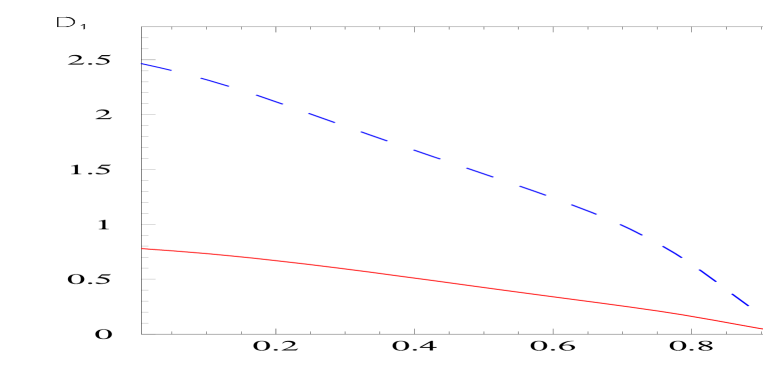
FIG. 5.: The FF $D_{1}(z)$ (left) and $H_{1\,(R)}^{{<\kern-2.10002pt{\scriptscriptstyle)}}}(z)$ (right). Solid line for $N_{q\rho}=0.9$ GeV³, and the integral (70) amounting to 0.14; dashed line for $N_{q\rho}=1.6$ GeV³, and the integral equals 0.48.

IV Numerical Results

In the remainder of the paper, we present numerical results in the context of the spectator model for both the process-independent FF and the SSA of Eqs. (97) and (98) for semi-inclusive lepton-nucleon DIS. Considering different possible scenarios for $h_{1}$, we discuss the implications for an experimental search for transversity.

The input parameters of the calculation can basically be grouped in three classes:

• values of masses and coupling constants taken from phenomenology, as $m_{\pi}=0.139$ GeV, $m_{\rho}=0.785$ GeV, with $f_{\rho\pi\pi}$ and $\Gamma_{\rho}$ as described in Sec. III B and Sec. III A, respectively;

• values consistent with other works on the spectator model and the constituent quark model, as $\Lambda_{\pi}=0.4$ GeV, $\Lambda_{\rho}=0.5$ GeV and $m_{q}=0.34$ GeV [18, 14];

• parameters, such as $N_{q\pi}$ and $N_{q\rho}$, without constraints that are firmly established, or at least usually adopted, in the literature.

As previously anticipated in Sec. III B, the last ones are constrained using the integral (70) and the proportionality (73) derived from the Goldberger-Treiman relation. All results will be plotted according to two extreme scenarios, where the integral (70) amounts to 0.14 ($N_{q\rho}=0.9$ GeV³, corresponding to solid lines in the figures) and 0.48 ($N_{q\rho}=1.6$ GeV³, corresponding to dashed lines in the figures). Because of the high degree of arbitrariness due to the lack of any data, the results should be interpreted as the indication not only of the sensitivity of the considered observables to the input parameters, but also of the degree of uncertainty that can be reached within the spectator model. In the same spirit, when dealing with the SSA of Eqs. (97,98), $f_{1}$ and $h_{1}$ are calculated consistently within the spectator model [18] or, alternatively, $f_{1}$ and $g_{1}$ are taken from consistent parametrizations and $h_{1}$ is calculated again according to two extreme scenarios: the nonrelativistic prediction $h_{1}=g_{1}$ or the saturation of the Soffer inequality, $h_{1}=(f_{1}+g_{1})/2$. The parametrizations for $f_{1},g_{1},$ are extracted at the same lowest possible scale ($Q^{2}=0.8$ GeV²), consistently with the valence quark approximation assumed for the calculation of the FF.

In Fig. 5 the integrated $D_{1}^{u}(z)$ and $H_{1\,(R)}^{{<\kern-2.10002pt{\scriptscriptstyle)}}\,u}(z)$ are shown. Again, we recall that the solid line corresponds to a weaker $q\rho q$ coupling than the dashed line. The choice of the form factors at the vertices also guarantees the regular behaviour at the end points $z=0,1$. The strongest asymmetry in the fragmentation (recall that $H_{1}^{{<\kern-2.10002pt{\scriptscriptstyle)}}}$ is defined as the probability difference for the fragmentation to proceed from a quark with opposite transverse polarizations) is reasonably reached at $z\sim 0.4$. Once again, we stress that this result, particularly its persistent negative sign, does not depend on a specific hard process and can influence the corresponding azimuthal asymmetry.

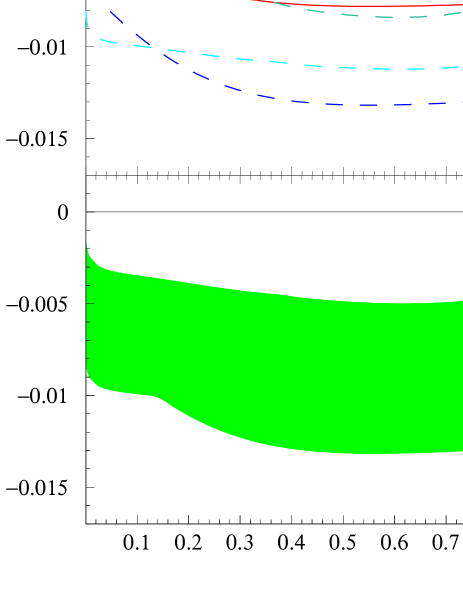
FIG. 6.: The SSA of Eq. (97). In the upper plot, solid lines and dashed lines as in Fig. 5. Label SP stands for DF calculated in the spectator model [18]. Labels NR and SO indicate $f_{1}$ from Ref. [23] and $g_{1}$ from Ref. [24], but with $h_{1}=g_{1}$ and $h_{1}=(f_{1}+g_{1})/2$, respectively. In the lower plot, the corresponding uncertainty band is shown (see text).

In fact, the SSA (97) and (98) for two-pion inclusive lepton-nucleon DIS as shown in Figs. 6 and 7, respectively, turn out to be negative due to the sign of $H_{1}^{{<\kern-2.10002pt{\scriptscriptstyle)}}\,u}$. The solid and dashed lines again refer to the weaker or stronger $q\rho q$ couplings in the FF, respectively. For each parametrization, three different choices of DF are shown. The label SP refers to the DF calculated in the spectator model [18]. The label NR indicates that $f_{1}$ and $g_{1}$ are taken consistently from the leading-order parametrizations of Ref. [23] and Ref. [24], respectively, with $h_{1}=g_{1}$. The label SO indicates the same parametrizations but with the Soffer inequality saturated, i.e. $h_{1}=(f_{1}+g_{1})/2$. In the lower plot of each figure the “uncertainty band” is shown as a guiding line. It is built by taking, for each $z$ or $M_{h}$, the maximum and the minimum among the six curves displayed in the corresponding upper plot. The first obvious comment is that even the simple mechanism described in Fig. 4 produces a measurable asymmetry. For the HERMES experiment the size of the asymmetry may be at the lower edge of possible measurements, given the observed rather small average multiplicity which does not favor the detection of two pions in the final state. On the other hand, the planned transversely polarized target clearly will improve the situation of azimuthal spin-asymmetry measurements compared to the present one. COMPASS or possible future experiments at the ELFE, TESLA-N, or EIC facilities will have less problems because of higher counting rates. The second important result is that the sensitivity of the SSA to the parameters of the model calculation for the FF and to the different parametrizations for the DF is weak enough that the unambigous message of a negative asymmetry emerges through all the range of both $x$ and $m_{\rho}-\Gamma_{\rho}/2=0.69$ GeV $\leq M_{h}\leq m_{\rho}+\Gamma_{\rho}/2=0.84$ GeV. In particular, we do not find any change in sign for $A^{\sin\phi}_{M_{h}}$, contrary to what is predicted in Ref. [13].

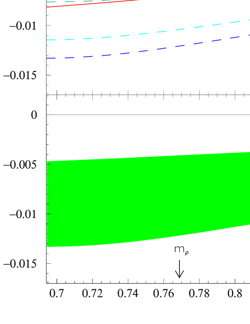
FIG. 7.: The SSA of Eq. (98). In the upper plot, solid lines and dashed lines as in Fig. 5. Labels and meaning of lower plot as in Fig. 6.

V Outlooks

In this paper we have discussed a way for addressing the transversity distribution $h_{1}$ that we consider most advantageous compared to other strategies discussed in the literature. At present, the SSA seem anyway preferable to the DSA. But the fragmentation of a transversely polarized quark into two unpolarized leading hadrons in the same current jet looks less complicated than the Collins effect, both experimentally and theoretically. Collinear factorization implies an exact cancellation of the soft divergencies, avoiding any dilution of the asymmetry because of Sudakov form factors, and in principle makes the QCD evolution simpler, though we have not addressed this subject in the present paper. The new effect, that allows for the extraction of $h_{1}$ at leading twist through the new interference FF $H_{1}^{{<\kern-2.10002pt{\scriptscriptstyle)}}}$, relates the transverse polarization of the quark to the transverse component of the relative momentum of the hadron pair via a new azimuthal angle. This is the only key quantity to be determined experimentally, while the Collins effect requires the determination of the complete transverse momentum vector of the detected hadron.

We have shown also quantitative results for $H_{1}^{{<\kern-2.10002pt{\scriptscriptstyle)}}}$ in the case of $\pi^{+}\pi^{-}$ detection, and the related SSA for the example of lepton-nucleon scattering, because modelling the interference between different channels leading to the same final state is simpler than describing the Collins effect, where a microscopic knowledge of the structure of the residual jet is required. We have adopted a spectator model approximation for $\pi^{+}\pi^{-}$ with an invariant mass inside the $\rho$ resonance width, limiting the process to leading-twist mechanisms. The interference between the decay of the $\rho$ and the direct production of $\pi^{+}\pi^{-}$ is enough to produce sizeable and measurable asymmetries. Despite the theoretical uncertainty due to the arbitrariness in fixing the input parameters of the calculation of FF and in choosing the parametrizations for the DF, the unambigous result emerges that in the explored ranges in $x$ and invariant mass $M_{h}$ the SSA are always negative and almost flat.

Anyway, it should be stressed again that, even if there are good arguments for considering the mechanisms depicted in Fig. 4 a good representation of $\pi^{+}\pi^{-}$ production in the considered energy range, still the calculation has been performed at leading twist and in a valence-quark scenario. Therefore, higher-twist corrections and QCD evolution need to be explored before any realistic comparison with experiments could be attempted.

REFERENCES

- [1] J. P. Ralston and D. E. Soper, Nucl. Phys. B 152, 109 (1979).
- [2] R. L. Jaffe, hep-ph/9710465.
- [3] O. Martin, A. Schafer, M. Stratmann and W. Vogelsang, Phys. Rev. D 57, 3084 (1998).
- [4] R. L. Jaffe and X. Ji, Nucl. Phys. B 375, 527 (1992).
-
[5]
R. L. Jaffe and X. Ji,
Phys. Rev. Lett. 71, 2547 (1993);
D. Boer, hep-ph/0007047. - [6] J. Collins, Nucl. Phys. B 396, 161 (1993).
-
[7]
A. Airapetian et al. [HERMES Collaboration],
Phys. Rev. Lett. 84 (2000) 4047;
A. Airapetian et al. [HERMES Collaboration], Phys. Rev. D 64 (2001) 097101;
A. Bravar [Spin Muon Collaboration], Nucl. Phys. Proc. Suppl. 79 (1999) 520. - [8] D. Boer, Nucl. Phys. B 603, 195 (2001); and private communications.
- [9] A. Bianconi, S. Boffi, R. Jakob and M. Radici, Phys. Rev. D 62, 034008 (2000).
- [10] A. Bacchetta, R. Kundu, A. Metz and P. J. Mulders, Phys. Lett. B 506 (2001) 155
- [11] J. C. Collins and G. A. Ladinsky, hep-ph/9411444.
- [12] J. C. Collins, S. F. Heppelmann and G. A. Ladinsky, Nucl. Phys. B 420, 565 (1994).
- [13] R. L. Jaffe, Xuemin Jin and Jian Tang, Phys. Rev. Lett. 80, 1166 (1998).
- [14] A. Bianconi, S. Boffi, R. Jakob and M. Radici, Phys. Rev. D 62, 034009 (2000).
- [15] V. Barone, A. Drago and P. G. Ratcliffe, hep-ph/0104283.
-
[16]
D. E. Soper,
Phys. Rev. D 15, 1141 (1977);
D. E. Soper, Phys. Rev. Lett. 43, 1847 (1979);
J. C. Collins and D. E. Soper, Nucl. Phys. B 194, 445 (1982);
R. L. Jaffe, Nucl. Phys. B 229, 205 (1983). -
[17]
H. Meyer and P. J. Mulders,
Nucl. Phys. A 528, 589 (1991);
W. Melnitchouk, A. W. Schreiber and A. W. Thomas, Phys. Rev. D 49, 1183 (1994);
J. Rodrigues, A. Henneman and P. J. Mulders, nucl-th/9510036. - [18] R. Jakob, P. J. Mulders and J. Rodrigues, Nucl. Phys. A 626, 937 (1997).
- [19] B. L. Ioffe, V. A. Khoze and L. N. Lipatov, Hard Processes, Vol. 1 (Elsevier, Amsterdam, 1984).
-
[20]
L. Y. Glozman, Z. Papp, W. Plessas, K. Varga and R. F. Wagenbrunn,
Phys. Rev. C 57 (1998) 3406;
R. F. Wagenbrunn, L. Y. Glozman, W. Plessas and K. Varga, Nucl. Phys. A 663&664 (2000) 703. - [21] T. E. Ericson and W. Weise, Pions in Nuclei (Clarendon Press, Oxford, 1988).
- [22] M. R. Pennington, hep-ph/9905241.
- [23] M. Glück, E. Reya and A. Vogt, Eur. Phys. J. C 5, 461 (1998).
- [24] M. Glück, E. Reya, M. Stratmann and W. Vogelsang, Phys. Rev. D 53, 4775 (1996).