PARAMETRIZATION OF THE ENERGY SPECTRUM IN THE TRITIUM BETA DECAY.
J. STUDNIK AND M. ZRAŁEK
Department of Field Theory and Particle Physics,
Institute of Physics, University of Silesia,
Uniwersytecka 4, PL-40-007 Katowice, Poland
Abstract
Taking into account
mixings among neutrino states, the end of the energy spectrum of the electron in the tritium beta decay is investigated.
It is shown that for real energy resolutions of a spectrometer, eV, the effective electron neutrino mass
should [not] be taken in the
form
.
Last atmospheric and solar experiments convince us that neutrinos are massive particles. However, the problem of absolute values of
their masses is still waiting for a solution. Apparently three kinds of neutrino experiments have a chance to determine the light neutrino masses.
These are:
1.
neutrino oscillation experiments,
2.
the tritium beta decay experiment,
3.
neutrinoless double beta decay experiments.
Among them the tritium decay
(1)
is of great importance. Here the end of the electron energy spectrum in the absence of the lepton mixing is described by [1]
(2)
is the electron kinematic energy , eV,
and
(3)
where is the Fermi constant, is the Cabibbo angle and M is the nuclear matrix element. is neutrino mass independent,
smooth function of , which takes into account radiative corrections to the produced final state electron
(see [1] for details). The effective mass of the produced neutrino is determined,
regardless of the fact if it is a Dirac or a Majorana particle.
Presently only the upper limit on is available. Two experiments in Mainz [2] and Troitsk [3] have recently found
(4)
(5)
The real problem is how this effective mass , extracted from the experiment, is connected to the realistic neutrino masses .
In the case of three light neutrinos (i=1,2,3) which mix (),
the spectrum of the electron energy is given by [4]
(6)
is the step function.
This formula
depends on five parameters, namely three neutrino masses and two mixings because .
If only the upper bound on is determined (present situation, Eq. 4) then a precise relation
(7)
is not so important. However, future experiments, as KATRIN [5] with the sensitivity
have a chance to find and then a form of Eq. 7 becomes
crucial for neutrinos mass determination.
Two parametrizations have been suggested in literature.
The first one [6]
(8)
is a result of Taylor expansion of the spectrum ( 6) around the point
follows from the approximation of the precise distribution (Eq. 6) by the effective one (Eq. 2) near
the end of the electron energy spectrum . We would like to elucidate the situation and decide which parametrization,
( 8) or ( 10) is better and should be used for future neutrinos mass determination.
Among five parameters and only one is actually unknown, it is the mass of the lightest one .
From neutrino oscillation experiments the mixing matrix elements , (i=1,2,3) and
are determined. For the LMA MSW solution of the solar neutrino problem the best fit values are [8]
(11)
and . Atmospheric neutrino oscillations give [8],
[9]. Uncertainties in the determination of the oscillation parameters from solar neutrino experiments are large [8],
but our main conclusions depend only weakly on them. The masses of heavier neutrinos are the function of the lightest neutrino
(12)
(13)
As is a smooth function of at the end of spectrum,
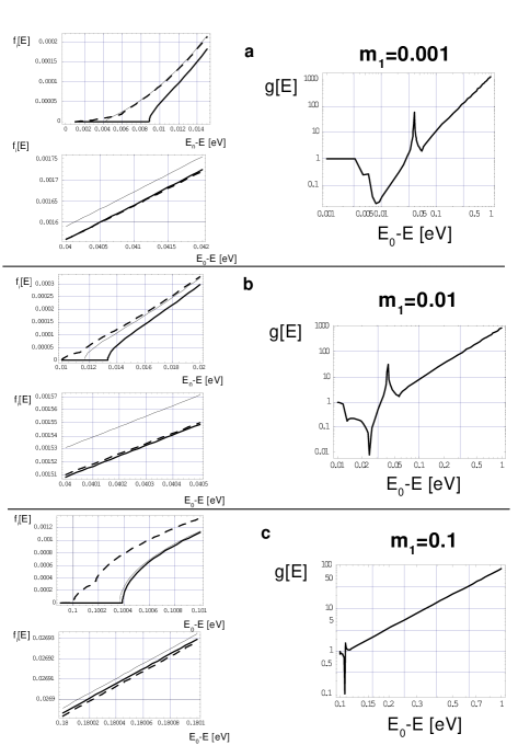
we can approximate . Then we can plot scaled energy distribution as:
(14)
In Fig. 1 the full (Eq. 6) and two effective distributions
( with and with ) are depicted as a function of energy for three particular values of the lightest neutrino
masses ( and ).
To compare both approximations, the ratio
(15)
is also shown.
We can see that for small values of the effective distribution with approximates the full spectrum in a better way
. For larger , , and gives better result. This conclusion is general, independent of the lightest neutrino mass
and values of the other oscillation parameters.
To answer the question which effective neutrino mass or should be used in future experimental searches,
the number of events in a possible small interval which still can be resolved by a detector
(16)
should be calculated. The integral
(17)
can be done analytically,
(18)
(19)
and
(20)
with
(21)
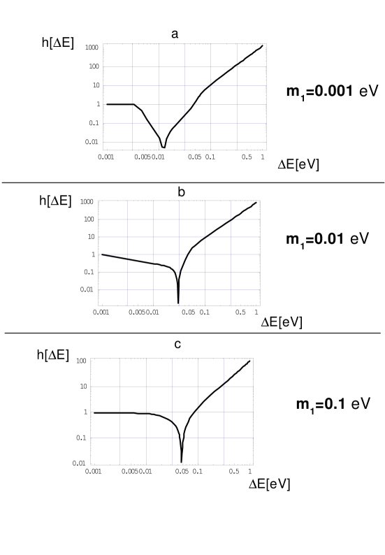
To compare both approximate spectra the ratio
(22)
is plotted on Fig. 2
for three different neutrino masses and .
We can see that independently of chosen and for , .
We know that [10]. It will be very difficult to get such a small energy spectrum resolution.
So, let us conclude. In practice , and approximate spectrum with should be used
in future searches of neutrino masses in the tritium decay.
FIG. 1.: The scaled electron energy distribution at the end of the spectrum for decay for three different masses of the lightest neutrino (a) eV, (b) eV, (c) eV. descibes the full (dashed line) and (i=1,2) describes approximate effective energy distribution for (tick solid line) and (thin solid line). The function g(E) compare both approximations (see text).FIG. 2.: h() as a function of for minimal neutrino mass (a) , (b) , (c) .
Acknowledgments
This work was supported by the Polish Committee for Scientific Research under Grant Nos. 2P03B05418 and 5P03B08921.
REFERENCES
[1] see e.g W. Kuandig et al., in “Neutrino Physics” ed. by K. Winter, Cambridge Univ. Press 1991, p. 144; F. Boehm, P. Vogel “ Physics of massive neutrinos”, Published by Press Syndicate of the University of Cambridge 1987, 1992 .
[2]J. Bonn, et al, Nucl. Phys.B 91 (2001)273.
[3]V. M. Lobashev, Nucl. Phys.B 91 (2001)273.
[4]R. E. Shrock, Phys. Lett.B 96 (1980) 159.
[5]V. Aseev et al. http://www.hep.anl.gov/ndk/hypertext/mumi/html, A. Osipowicz at.al. [hep-ex/0109033]
[6]F. Vissani,
hep-ph/0102235.
[7]Y. Farzan, O. L. Peres and A. Y. Smirnov,
hep-ph/0105105.
[8]
M. C. Gonzalez-Garcia, M. Maltoni, C. Pena-Garay and J. W. Valle,
Phys. Rev. D 63, 033005 (2001)
[hep-ph/0009350].