Light-front quark model analysis of rare $B\to K\ell^{+}\ell^{-}$ decays

Abstract

Using the light-front quark model, we calculate the transition form factors, decay rates, and longitudinal lepton polarization asymmetries for the exclusive rare $B\to K\ell^{+}\ell^{-}$($\ell=e,\mu,\tau$) decays within the standard model. Evaluating the timelike form factors, we use the analytic continuation method in $q^{+}=0$ frame to obtain the form factors $F_{+}$ and $F_{T}$, which are free from zero-mode. The form factor $F_{-}$ which is not free from zero-mode in $q^{+}=0$ frame and contaminated by the higher(or nonvalence) Fock states in $q^{+}\neq 0$ frame is obtained from an effective treatment for handling the nonvalence contribution based on the Bethe-Salpeter formalism. The covariance(i.e. frame-independence) of our model calculation is discussed. We obtain the branching ratios for ${\rm BR}(B\to K\ell^{+}\ell^{-})$ as $4.96\times 10^{-7}|V_{ts}/V_{cb}|^{2}$ for $\ell=e,\mu$ and $1.27\times 10^{-7}|V_{ts}/V_{cb}|^{2}$ for $\ell=\tau$.

I Introduction

The upcoming and currently operating B factories BaBar at SLAC, Belle at KEK, LHCB at CERN and B-TeV at Fermilab as well as the planned $\tau$-Charm factory CLEO at Cornell make the precision test of standard model(SM) and beyond SM ever more promising [1]. Especially, a stringent test on the unitarity of Cabibbo-Kobayashi-Maskawa (CKM) mixing matrix in SM will be made by these facilities. Accurate analyses of exclusive semileptonic B-decays as well as rare B-decays are thus strongly demanded for such precision tests. One of the physics programs at the B factories is the exclusive rare B decays induced by the flavor-changing neutral current(FCNC) transition. Since in the standard model they are forbidden at tree level and occur at the lowest order only through one-loop (Penguin) diagrams [2, 3, 4, 5, 6], the rare B decays are well suited to test the SM and search for physics beyond the SM. While the experimental tests of exclusive decays are much easier than those of inclusive ones, the theoretical understanding of exlcusive decays is complicated mainly due to the nonperturbative hadronic form factors entered in the long distance nonperturbative contributions. The calculations of hadronic form factors for rare B decays have been investigated by various theoretical approaches, such as relativistic quark model [7, 8, 9, 10], heavy quark theory [11], three point QCD sum rules [12], light cone QCD sum rule [13, 14, 15, 16], and chiral perturbation theory [17, 18]. Perhaps, one of the most well-suited formulations for the analysis of exclusive processes involving hadrons may be provided in the framework of light-front quantization [19].

The aim of the present work is to calculate the hadronic form factors, decay rates and the longitudinal lepton polarization asymmetries for $B\to K\ell^{+}\ell^{-}$($\ell=e,\mu$, and $\tau$) decays within the framework of the SM, using our light-front constituent quark model(LFCQM or simply LFQM)) [20, 21, 22, 23] based on the LF quantization. The longitudinal lepton polarization, as another parity-violating observable, is an important asymmetry [24] and could be measured by the above mentioned B factories. In particular, the $\tau$ channel would be more accessible experimentally than $e$- or $\mu$-channels since the lepton polarization asymmetries in the SM are known to be proportional to the lepton mass. Although some recent works [25] have studied the lepton polarizations using the general form of the effective Hamiltonian including all possible forms of interactions, we shall analyze them within the SM as many others did.

Our LFQM [20, 21, 22, 23] used in the present analysis has several salient features compared to other LFQM [7, 8] analysis: (1) We have implemented the variational principle to the QCD motivated effective LF Hamiltonian to enable us to analyze the meson mass spectra as well as various wavefunction-related observables such as decay constants, electromagnetic form factors of mesons in spacelike ($q^{2}<0$) region [20]. (2) We have performed the analytical continuation of the weak form factors from spacelike region to the entire (physical) timelike region to obtain the weak form factors for the exclusive semileptonic decays of pseudoscalar mesons [21]. (3) We have recently presented in [22] an effective treatment of handling the higher Fock state (or nonvalence) contribution to the weak form factor in $q^{+}>0$ frames, based on the Bethe-Salpeter(BS) formalism (see also [23]).

The explicit demonstration of our analytic continuation method using the exactly solvable model of ($3+1$)-dimensional scalar field theory model can be found in [26]. The Drell-Yan-West ($q^{+}$=$q^{0}$+$q^{z}$=0) frame is useful because only valence contributions are needed as far as the “$+$”-component of the current is used. Our analytic solution in the $q^{+}$=0 frame as a direct application to the timelike region differs from the method used in [7, 8] where the authors used a simple parametric formula extracted from the small $q^{2}$ behavior of a form factor. However, some of the form factors in timelike exclusive processes receive higher Fock state contributions(i.e. zero-mode in $q^{+}=0$ frame or nonvalence contribution in $q^{+}\neq 0$ frame) within the framework of LF quantization. Thus, it is necessary to include either zero-mode contribution(if working in $q^{+}=0$ frame) or the nonvalence contribution (if working in $q^{+}\neq 0$ frame) to obtain such form factors. Specifically, in the present analysis of exclusive rare $B\to K\ell^{+}\ell^{-}$ decays, three independent hadronic form factors, i.e. $F_{+}(q^{2})$, $F_{-}(q^{2})$ from the $V$-$A$(vector-axial vector) current, and $F_{T}(q^{2})$ from the tensor current, are needed. While the two form factors $F_{+}$ and $F_{T}$ can be obtained from only valence contribution in $q^{+}=0$ frame without encountering the zero-mode complication [27], it is necessary to include the nonvalence contribution for the calculation of the form factor $F_{-}$. Our effective method[22] of calculating novalence contributions has been shown to be quite reliable by checking the covariance of the model. Thus, we utilize both the analytic method in $q^{+}=0$ frame to obtain ($F_{+},F_{T}$) and the effective method in $q^{+}>0$ frame to obtain $F_{-}$, respectively.

The paper is organized as follows. In Sec. II, we discuss the standard model effective Hamiltonian for the exclusive rare $B\to K\ell^{+}\ell^{-}$ decays and reproduce the QCD Wilson coefficients necessary in our analysis. The formulas of the hadronic form factors, differential decay rates, and the longitudinal lepton polarization asymmetries are also introduced in this section. In Sec. III, we calculate the weak form factors $F_{+}(q^{2}),F_{-}(q^{2})$ and $F_{T}(q^{2})$ using our LFQM. To obtain $F_{+}(q^{2})$ and $F_{T}(q^{2})$, we use the $q^{+}=0$ frame (i.e. $q^{2}=-\vec{q}^{2}_{\perp}<0$) and then analytically continue the results to the timelike $q^{2}>0$ region by changing $q_{\perp}$ to $iq_{\perp}$ in the form factors. The form factor $F_{-}(q^{2})$ is obtained from our effective method [22] in purely longitudinal $q^{+}>0$ frames (i.e. $q^{2}=q^{+}q^{-}>0$). In Sec. IV, our numerical results, i.e. the form factors, decay rates, and the longitudinal lepton polarization asymmetries for $B\to K\ell^{+}\ell^{-}$ decays, are presented and compared with the experimental data as well as other theoretical results. Summary and discussion of our main results follow in Sec. V. In the Appendix A, we list the QCD Wilson coefficients necessary for the rare $B\to K$ transition. In the Appendix B, we show the derivation of the differential decay rate for $B\to K\ell^{+}\ell^{-}$ in the case of nonzero lepton($m_{\ell}\neq 0$) mass. In Appendix C, we show the generic form of our analytic solutions for the weak form factors in timelike region.

II Overview of Effective Hamiltonian in Operator Basis

The rare $b\to s\ell^{+}\ell^{-}$ decay process can be represented in terms of the Wilson coefficients of the effective Hamiltonian obtained after integrating out the heavy top quark and the $W^{\pm}$ bosons [2], i.e.

$${\cal H}_{\rm eff}=\frac{4G_{F}}{\sqrt{2}}V_{tb}V^{*}_{ts}\sum_{i}C_{i}(\tilde{\mu})O_{i}(\tilde{\mu}),$$ (1)

where $G_{F}$ is the Fermi constant, $V_{ij}$ are the CKM matrix elements and $C_{i}(\tilde{\mu})$ are the Wilson coefficients. It is known that the Wilson coefficients $C_{3}-C_{6}$ of QCD penguin operators $O_{3}-O_{6}$ are small enough to be neglected and also the operator $O_{8}$($\sim G^{a}_{\mu\nu}$, strong interaction field strength tensor) does not contribute to $b\to s\ell^{+}\ell^{-}$ transition. Thus, the relevant basis operators $O_{i}(\tilde{\mu})$ to the rare $b\to s\ell^{+}\ell^{-}$ decay are

$$O_{1} = (\bar{s}_{\alpha}\gamma^{\mu}P_{L}b_{\alpha})(\bar{c}_{\beta}\gamma^{\mu}P_{L}c_{\beta}),$$ (2)

$$O_{2} = (\bar{s}_{\alpha}\gamma^{\mu}P_{L}b_{\beta})(\bar{c}_{\beta}\gamma^{\mu}P_{L}c_{\alpha}),$$ (3)

$$O_{7} = \frac{e}{16\pi^{2}}m_{b}(\bar{s}_{\alpha}\sigma_{\mu\nu}P_{R}b_{\alpha})F^{\mu\nu},$$ (4)

$$O_{9} = \frac{e^{2}}{16\pi^{2}}(\bar{s}_{\alpha}\gamma^{\mu}P_{L}b_{\alpha})(\bar{\ell}\gamma_{\mu}\ell),$$ (5)

$$O_{10} = \frac{e^{2}}{16\pi^{2}}(\bar{s}_{\alpha}\gamma^{\mu}P_{L}b_{\alpha})(\bar{\ell}\gamma_{\mu}\gamma_{5}\ell),$$ (6)

where $P_{L(R)}=(1\mp\gamma_{5})/2$ is the chiral projection operator and $F^{\mu\nu}$ is the electromagnetic interaction field strength tensor. The Lorentz and color indices are denoted as $\mu$(and $\nu$) and $\alpha$(and $\beta$), respectively. The renormalization scale $\tilde{\mu}$ in Eq. (1) is usually chosen to be $\tilde{\mu}\simeq m_{b}$ in order to avoid large logarithms, ln($M_{W}/m_{b}$), in the matrix elements of the operators $O_{i}$. The Wilson coefficients $C_{i}(m_{b})$ determined by the renormalization group equations(RGE) from the perturbative values $C_{i}(M_{W})$ are given in the literature(see, for example [3, 4]).

Since the operators $O_{1}$ and $O_{2}$ contribute to $b\to s\ell^{+}\ell^{-}$ through $c\bar{c}$-loops which again couple to $\ell^{+}\ell^{-}$ through virtual photon, they can be incorporated into an “effective” $O_{9}$. The resulting effective Hamiltonian in Eq. (1) has the following structure(neglecting the strange quark mass)

$${\cal H}^{\ell^{+}\ell^{-}}_{\rm eff} = \frac{4G_{F}}{\sqrt{2}}\frac{e^{2}}{16\pi^{2}}V^{*}_{ts}V_{tb}\biggl{[}-\frac{2iC_{7}(m_{b})m_{b}}{q^{2}}\bar{s}\sigma_{\mu\nu}q^{\nu}P_{R}b\bar{\ell}\gamma^{\mu}\ell$$ (7)

$$+ C^{\rm eff}_{9}(m_{b})\bar{s}\gamma_{\mu}P_{L}b\bar{\ell}\gamma^{\mu}\ell+C_{10}(m_{b})\bar{s}\gamma_{\mu}P_{L}b\bar{\ell}\gamma^{\mu}\gamma_{5}\ell\biggr{]}.$$ (8)

The effective Wilson coefficient $C^{\rm eff}_{9}$($\hat{s}$=$q^{2}/m^{2}_{b}$) is given by [6, 28, 29]

$$C^{\rm eff}_{9}(\hat{s}) \equiv \tilde{C}^{\rm eff}_{9}(\hat{s})+Y_{\rm LD}(\hat{s}),$$ (10)

$$= C_{9}\biggl{(}1+\frac{\alpha_{s}(\mu)}{\pi}\omega(\hat{s})\biggr{)}+Y_{\rm SD}(\hat{s})+Y_{\rm LD}(\hat{s}),$$ (11)

where the function $Y_{\rm SD}(\hat{s})$ is the one-loop matrix element of $O_{9}$, $Y_{\rm LD}(\hat{s})$ describes the long distance contributions due to the charmonium vector $J/\psi,\psi^{\prime},\cdots$ resonances via $B\to K(J/\psi,\psi^{\prime},\cdots)\to K\ell^{+}\ell^{-}$, and $\omega(\hat{s})$ represents the one-gluon correction to the matrix element of $O_{9}$. Their explicit forms are given in the literature [3, 4, 28, 29, 30] and also in the Appendix A of this work. For the numerical values of the Wilson coefficients and relevant parameters in obtaining Eq. (10), we use the results given by Refs. [29, 30]: $m_{t}=175$ GeV, $m_{b}=4.8$ GeV, $m_{c}=1.4$ GeV, $\alpha_{s}(M_{W})=0.12$, $\alpha_{s}(m_{b})=0.22$, $C_{1}=-0.26$, $C_{2}=1.11$, $C_{3}=0.01$, $C_{4}=-0.03$, $C_{5}=0.008$, $C_{6}=-0.03$, $C_{7}=-0.32$, $C_{9}=4.26$, and $C_{10}=-4.62$.

In Fig. 1, we plot the effective Wilson coefficient $C^{\rm eff}_{9}$ as a function of $\hat{s}$. As the real part of $C^{\rm eff}_{9}$, the thick(thin) solid line represents the result with(without) LD contribution, i.e. ${\rm Re}(C^{\rm eff}_{9})({\rm Re}(\tilde{C}^{\rm eff}_{9}))$. The imaginary (dotted line) part of $C^{\rm eff}_{9}$ is the result without LD contribution, ${\rm Im}(\tilde{C}^{\rm eff}_{9})$. In our numerical calculation of $C^{\rm eff}_{9}$(thick solid lines), we include two charmonium vector $J/\psi(1S)$ and $\psi^{\prime}(2S)$ resonances(see Appendix A). The cusp of Re($\tilde{C}^{\rm eff}_{9}$) at $\hat{s}=4(m_{c}/m_{b})^{2}\simeq 0.34$ as shown in Fig. 1 (thin line) is due to the $c\bar{c}$-loop contribution from $Y_{SD}(\hat{s})$[see Eqs. (A4) and (A8) in Appendix A]. In Fig. 1, one can also find that ${\rm Re}(\tilde{C}^{\rm eff}_{9})\gg{\rm Im}(\tilde{C}^{\rm eff}_{9})$.

FIG. 1.: The effective Wilson coefficient $C^{\rm eff}_{9}$ as a function of $\hat{s}=q^{2}/M^{2}_{B}$. As the real part of $C^{\rm eff}_{9}$, the thick(thin) solid line represents the results with(without) LD contribution, i.e. $C^{\rm eff}_{9}(\tilde{C}^{\rm eff}_{9})$. The imaginary (dotted line) part of $C^{\rm eff}_{9}$ is the result without LD contribution.

The long-distance contribution to the exclusive $B\to K$ decay is contained in the meson matrix elements of the bilinear quark currents appearing in ${\cal H}^{\ell^{+}\ell^{-}}_{\rm eff}$ given by Eq. (7). The matrix elements of the hadronic currents for $B\to K$ transition can be parametrized in terms of hadronic form factors as follows

$$J^{\mu} \equiv \langle K|\bar{s}\gamma^{\mu}P_{L}b|B\rangle=\frac{1}{2}[F_{+}(q^{2})P^{\mu}+F_{-}(q^{2})q^{\mu}],$$ (12)

and

$$J^{\mu}_{T} \equiv \langle K|\bar{s}i\sigma^{\mu\nu}q_{\nu}P_{R}b|B\rangle$$ (13)

$$= \frac{1}{2(M_{B}+M_{K})}[q^{2}P^{\mu}-(M^{2}_{B}-M^{2}_{K})q^{\mu}]F_{T}(q^{2}),$$ (14)

where $P=P_{B}+P_{K}$ and $q=P_{B}-P_{K}$ is the four-momentum transfer to the lepton pair and $4m^{2}_{l}\leq q^{2}\leq(M_{B}-M_{K})^{2}$. We use the convention $\sigma^{\mu\nu}=(i/2)[\gamma^{\mu},\gamma^{\nu}]$ for the antisymmetric tensor. Sometimes it is useful to express Eq. (12) in terms of $F_{+}(q^{2})$ and $F_{0}(q^{2})$, which are related to the exchange of $1^{-}$ and $0^{+}$, respectively, and satisfy the following relations:

$$F_{+}(0)=F_{0}(0),\;F_{0}(q^{2})=F_{+}(q^{2})+\frac{q^{2}}{M^{2}_{B}-M^{2}_{K}}F_{-}(q^{2}).$$ (15)

With the help of the effective Hamiltonian in Eq. (7) and Eqs. (12) and (13), the transition amplitude for the $B\to K\ell^{+}\ell^{-}$ decay can be written as

$${\cal M} = \langle K\ell^{+}\ell^{-}|{\cal H}_{\rm eff}|B\rangle$$ (16)

$$= \frac{4G_{F}}{\sqrt{2}}\frac{\alpha}{4\pi}V^{*}_{ts}V_{tb}\biggl{\{}\biggl{[}C^{\rm eff}_{9}J_{\mu}-\frac{2m_{b}}{q^{2}}C_{7}J^{T}_{\mu}\biggr{]}\bar{\ell}\gamma^{\mu}\ell$$ (18)

$$\hskip 71.13188pt+C_{10}J_{\mu}\bar{\ell}\gamma^{\mu}\gamma_{5}\ell\biggr{\}},$$

where $\alpha=e^{2}/4\pi$ is the fine structure constant. The differential decay rate for the exlcusive rare $B\to K\ell^{+}\ell^{-}$ with nonzero lepton mass($m_{\ell}\neq 0$) is given by (see Appendix B for the detailed derivation)

$$\frac{d\Gamma}{d\hat{s}} = \frac{M^{5}_{B}G^{2}_{F}}{3\cdot 2^{9}\pi^{5}}\alpha^{2}|V^{*}_{ts}V_{tb}|^{2}\hat{\phi}^{1/2}\biggl{(}1-4\frac{\hat{m}_{\ell}}{\hat{s}}\biggr{)}^{1/2}$$ (20)

$$\times\biggl{[}\hat{\phi}\biggl{(}1+2\frac{\hat{m}_{\ell}}{\hat{s}}\biggr{)}F_{T+}+6\frac{\hat{m}_{\ell}}{\hat{s}}F_{0+}\biggr{]},$$

where

$$F_{T+} = |C^{\rm eff}_{9}F_{+}-\frac{2C_{7}}{1+\sqrt{\hat{r}}}F_{T}|^{2}+|C_{10}|^{2}|F_{+}|^{2},$$ (21)

$$F_{0+} = |C_{10}|^{2}[(1-\hat{r})^{2}|F_{0}|^{2}-\hat{\phi}|F_{+}|^{2}],$$ (22)

$$\hat{\phi} = (\hat{s}-1-\hat{r})^{2}-4\hat{r},$$ (23)

with $\hat{s}=q^{2}/M^{2}_{B}$, $\hat{m}_{\ell}=m^{2}_{\ell}/M^{2}_{B}$, and $\hat{r}=M^{2}_{K}/M^{2}_{B}$. We used $m_{b}\simeq M_{B}$ in derivation of Eq. (20). Note also from Eqs. (20) and (21) that the form factor $F_{-}(q^{2})$(or $F_{0}(q^{2})$) contributes only in the nonzero lepton($m_{\ell}\neq 0$) mass limit. Dividing Eq. (20) by the total width of the $B$ meson, which is estimated to be [7, 34]

$$\Gamma_{\rm tot}=\frac{fM^{5}_{B}G^{2}_{F}}{192\pi^{3}}|V_{cb}|^{2},\;f\simeq 3.0,$$ (24)

one can obtain the differential branching ratio $dBR(B\to K\ell^{+}\ell^{-})/d\hat{s}=(d\Gamma(B\to K\ell^{+}\ell^{-})/\Gamma_{\rm tot})/d\hat{s}$ .

As another interesting observable, the longitudinal lepton polarization asymmetry(LPA), is defined as

$$P_{L}(\hat{s})=\frac{d\Gamma_{h=-1}/d\hat{s}-d\Gamma_{h=1}/d\hat{s}}{d\Gamma_{h=-1}/d\hat{s}+d\Gamma_{h=1}/d\hat{s}},$$ (25)

where $h=+1(-1)$ denotes right (left) handed $\ell^{-}$ in the final state. From Eq. (20), one obtains for $B\to K\ell^{+}\ell^{-}$

$$P_{L}(\hat{s})=\frac{2\biggl{(}1-4\frac{\hat{m}_{\ell}}{\hat{s}}\biggr{)}^{1/2}\hat{\phi}C_{10}F_{+}\biggl{[}F_{+}{\rm Re}C^{\rm eff}_{9}-\frac{2C_{7}}{1+\sqrt{\hat{r}}}F_{T}\biggr{]}}{\biggl{[}\hat{\phi}\biggl{(}1+2\frac{\hat{m}_{\ell}}{\hat{s}}\biggr{)}F_{T+}+6\frac{\hat{m}_{\ell}}{\hat{s}}F_{0+}\biggr{]}}.$$ (26)

Note that our formulas for the differential decay rate in Eq. (20) and the LPA in Eq. (26) are written in terms of ($F_{+},F_{0},F_{T}$) instead of ($F_{+},F_{-},F_{T}$) as obtained in Refs. [8, 10]. However, our formulas and those in [8, 10] are equivalent with each other once we rearrange our formulas in terms of ($F_{+},F_{-},F_{T}$). One nice feature of using $F_{0}$ in the decay rate formula is to separate the $F_{0}$ contribution from the total rate as we shall show later.

III Form Factor Calculation in Light-Front Quark Model

A Analytic calculation in $q^{+}=0$ frame

As shown in Eq. (20), only two weak form factors $F_{+}(q^{2})$ and $F_{T}(q^{2})$ are necessary for the massless($m_{\ell}=0$) rare exclusive semileptonic $b\to s\ell^{+}\ell^{-}$ process. The form factors $F_{+}(q^{2})$ and $F_{T}(q^{2})$ can be obtained in $q^{+}=0$ frame with the “good” component of currents, i.e. $\mu=+$, without encountering zero-mode contributions [27]. Thus, we shall perform our light-front quark model calculation in the $q^{+}=0$ frame, where $q^{2}=q^{+}q^{-}-{\vec{q}_{\perp}}^{2}=-\vec{q}^{2}_{\perp}<0$, and then analytically continue the form factors $F_{i}(\vec{q}^{2}_{\perp})(i=+,T)$ in spacelike region to the timelike $q^{2}>0$ region by changing $\vec{q}_{\perp}$ to $i\vec{q}_{\perp}$ in the form factor.

The quark momentum variables for $P_{B}(q_{1}\bar{q})\to P_{K}(q_{2}\bar{q})$ transitions in the $q^{+}=0$ frame are given by

$$p^{+}_{1} = (1-x)P^{+}_{1},\hskip 42.67912ptp^{+}_{\bar{q}}=xP^{+}_{1},$$ (27)

$${\vec{p}}_{1\perp} = (1-x){\vec{P}}_{1\perp}+{\vec{k}}_{\perp},\hskip 14.22636pt{\vec{p}}_{\bar{q}\perp}=x{\vec{P}}_{1\perp}-{\vec{k}}_{\perp},$$ (28)

$$p^{+}_{2} = (1-x)P^{+}_{2},\hskip 42.67912ptp^{\prime+}_{\bar{q}}=xP^{+}_{2},$$ (29)

$${\vec{p}}_{2\perp} = (1-x){\vec{P}}_{2\perp}+{\vec{k}^{\prime}}_{\perp},\hskip 14.22636pt{\vec{p}^{\prime}}_{\bar{q}\perp}=x{\vec{P}}_{2\perp}-{\vec{k}^{\prime}}_{\perp},$$ (30)

which require that $p^{+}_{\bar{q}}=p^{\prime+}_{\bar{q}}$ and ${\vec{p}}_{\bar{q}\perp}={\vec{p}^{\prime}}_{\bar{q}\perp}$. For $B\to K$ transitions, one has $m_{1}=m_{b}$, $m_{2}=m_{s}$, and $m_{\bar{q}}=m_{u}$. Our analysis for $b\to s\ell^{+}\ell^{-}$ decays will be carried out in this $q^{+}=0$ frame and the decaying hadron (B-meson) is at rest, i.e. ${\vec{P}}_{1\perp}=0$.

The matrix elements of the currents $J^{\mu}$ in Eq. (12) and $J^{\mu}_{T}$ in Eq. (13) are obtained by the convolution formula of the initial and final state light-front wave functions as follows

$$\langle P_{2}|\bar{q}_{2}\Gamma^{\mu}q_{1}|P_{1}\rangle = \sum_{{\lambda}^{\prime}s}\int d^{3}\vec{p}_{\bar{q}}\;\phi_{2}(x,{\vec{k}^{\prime}}_{\perp})\phi_{1}(x,{\vec{k}}_{\perp})$$ (32)

$$\times{\cal R}^{00^{\dagger}}_{\lambda_{2}\bar{\lambda}}\frac{\bar{u}_{\lambda_{2}}(p_{2})}{\sqrt{p^{+}_{2}}}\Gamma^{\mu}\frac{u_{\lambda_{1}}(p_{1})}{\sqrt{p^{+}_{1}}}{\cal R}^{00}_{\lambda_{1}\bar{\lambda}},$$

where $\Gamma^{\mu}=\gamma^{\mu}P_{L}$ for $J^{\mu}$ in Eq. (12) and $i\sigma^{\mu\nu}q_{\nu}P_{R}$ for $J^{\mu}_{T}$ in Eq. (13), respectively. The measure $[d^{3}\vec{p}_{\bar{q}}]$ in Eq. (32) is written in terms of light-front variables as

$$d^{3}\vec{p}_{\bar{q}} = P^{+}_{1}dxd^{2}\vec{k}_{\perp}\sqrt{\frac{\partial k^{\prime}_{z}}{\partial x}}\sqrt{\frac{\partial k_{z}}{\partial x}},$$ (33)

where ${\partial k_{z}}/{\partial x}$ is the Jacobian of the variable transformation $\{x,{\vec{k}}_{\perp}\}\to{\vec{k}}=(k_{z},{\vec{k}}_{\perp})$ defined by

$$\frac{\partial k_{z}}{\partial x} = \frac{M_{0}}{4x(1-x)}\biggl{[}1-\biggl{(}\frac{m^{2}_{q}-m^{2}_{\bar{q}}}{M^{2}_{0}}\biggr{)}^{2}\biggr{]},$$ (34)

$$M^{2}_{0} = \frac{m^{2}_{q}+\vec{k}^{2}_{\perp}}{1-x}+\frac{m^{2}_{\bar{q}}+\vec{k}^{2}_{\perp}}{x}.$$ (35)

The spin-orbit wave function ${\cal R}^{JJ_{z}}_{\lambda_{q},\lambda_{\bar{q}}}(x,{\vec{k}}_{\perp})$ is obtained by the interaction-independent Melosh transformation. The explicit covariant form for a pseudoscalar($J=0,J_{z}=0$) meson is given by

$${\cal R}^{J=0,J_{z}=0}_{\lambda_{q},\lambda_{\bar{q}}}(x,{\vec{k}}_{\perp})=\frac{\bar{u}(p_{q},\lambda_{q})\gamma^{5}v(p_{\bar{q}},\lambda_{\bar{q}})}{\sqrt{2}\sqrt{M^{2}_{0}-(m^{2}_{q}-m^{2}_{\bar{q}})^{2}}},$$ (36)

where ${\lambda}^{\prime}s$ are light-front helicities. Our radial wave function is given by the gaussian trial function for the variational principle to the QCD-motivated effective light-front Hamiltonian [20]:

$$\phi(x,{\vec{k}}_{\perp})=\biggl{(}\frac{1}{\pi^{3/2}\beta^{3}}\biggr{)}^{1/2}\exp(-\vec{k}^{2}/2\beta^{2}),$$ (37)

which is normalized as $\int d^{3}k|\phi(x,{\vec{k}}_{\perp})|^{2}=1$, where $\vec{k}^{2}=\vec{k}^{2}_{\perp}+k^{2}_{z}$ and $k_{z}$ is given by

$$k_{z}=(x-\frac{1}{2})M_{0}+\frac{m^{2}_{q}-m^{2}_{\bar{q}}}{2M_{0}}.$$ (38)

Then, the sum of the light-front spinors over the helicities in Eq. (32) are obtained as

$$\sum_{{\lambda}^{\prime}s}v_{\lambda_{\bar{q}}}^{\dagger}(p_{\bar{q}})\gamma^{5}\bar{u}_{\lambda_{2}}^{\dagger}(p_{2})\bar{u}_{\lambda_{2}}(p_{2})\Gamma^{\mu}u_{\lambda_{1}}(p_{1})\bar{u}_{\lambda_{1}}(p_{1})\gamma^{5}v_{\lambda_{\bar{q}}}(p_{\bar{q}})$$ (39)

$$={\rm Tr}\biggl{[}(\not\!p_{\bar{q}}-m_{\bar{q}})\gamma^{5}(\not\!p_{2}+m_{2})\Gamma^{\mu}(\not\!p_{1}+m_{1})\gamma^{5}\biggr{]}.$$ (40)

Using the matrix element of the “$+$” component of the currents($\mu=+$), and the particle on-mass shell condition, i.e. the light-front energy $p^{-}_{i}=(\vec{p}^{2}_{i\perp}+m^{2}_{i})/p^{+}_{i}$($i=1,2$ and $\bar{q}$) in Eq. (39), we obtain the weak form factors $F_{+}(\vec{q}_{\perp}^{2})$ and $F_{T}(\vec{q}_{\perp}^{2})$ as follows

$$F_{+}(\vec{q}_{\perp}^{2}) = \int^{1}_{0}dx\int d^{2}{\vec{k}}_{\perp}\sqrt{\frac{\partial k^{\prime}_{z}}{\partial x}}\sqrt{\frac{\partial k_{z}}{\partial x}}\phi_{2}(x,{\vec{k}^{\prime}}_{\perp})\phi_{1}(x,{\vec{k}}_{\perp})$$ (42)

$$\times\frac{A_{1}A_{2}+{\vec{k}}_{\perp}\cdot{\vec{k}^{\prime}}_{\perp}}{\sqrt{A_{1}^{2}+\vec{k}^{2}_{\perp}}\sqrt{A_{2}^{2}+\vec{k^{\prime}}^{2}_{\perp}}},$$

and

$$F_{T}(\vec{q}_{\perp}^{2}) = -\int^{1}_{0}dx\int d^{2}{\vec{k}}_{\perp}\sqrt{\frac{\partial k^{\prime}_{z}}{\partial x}}\sqrt{\frac{\partial k_{z}}{\partial x}}\phi_{2}(x,{\vec{k}^{\prime}}_{\perp})\phi_{1}(x,{\vec{k}}_{\perp})$$ (44)

$$\times\frac{M_{B}+M_{K}}{(1-x)\tilde{M}_{0}\tilde{M^{\prime}}_{0}}\biggl{[}(m_{2}-m_{1})\frac{\vec{k}_{\perp}\cdot\vec{q}_{\perp}}{\vec{q}^{2}_{\perp}}+A_{1}\biggr{]},$$

where $A_{i}=xm_{i}+(1-x)m_{\bar{q}}(i=1,2)$, $\tilde{M}_{0}=\sqrt{M^{2}_{0}-(m_{q}-m_{\bar{q}})^{2}}$, and ${\vec{k}^{\prime}}_{\perp}={\vec{k}}_{\perp}-x{\vec{q}}_{\perp}$. The primed factors in Eqs. (42) and (44) are the functions of final state momenta, e.g. $k^{\prime}_{z}=k^{\prime}_{z}(x,\vec{k^{\prime}}_{\perp})$ and $\tilde{M^{\prime}}_{0}=\tilde{M^{\prime}}_{0}(x,\vec{k^{\prime}}_{\perp})$. Since the weak form factors $F_{+}(\vec{q}^{2}_{\perp})$ in Eq. (42) and $F_{T}({\vec{q}_{\perp}}^{2})$ in Eq. (44) are defined in the spacelike($q^{2}<0$) region, we then analytically continue them to the timelike $q^{2}>0$ region by replacing $q_{\perp}$ with $iq_{\perp}$ in the form factors. We describe in Appendix C our procedure of analytic continuation of the weak form factors.

Our analytic solutions will be compared with the following parametric form used by many others [7, 8, 9, 13, 29]

$$F(q^{2})=\frac{F(0)}{1-\sigma_{1}q^{2}+\sigma_{2}q^{4}},$$ (46)

where the parameters $\sigma_{1}$ and $\sigma_{2}$ are determined by the first and second derivatives of $F(q^{2})$ at $q^{2}=0$.

B Effective calculation in $q^{+}>0$ frame

Our effective calculation of weak form factors is performed in the purely longitudinal momentum frame [22, 27] where $q^{+}>0$ and ${\vec{P}}_{1\perp}={\vec{P}}_{2\perp}=0$ so that the momentum transfer square $q^{2}=q^{+}q^{-}>0$ is timelike.

One can then easily obtain $q^{2}$ in terms of the momentum fraction $\alpha=P^{+}_{2}/P^{+}_{1}=1-q^{+}/P^{+}_{1}$ as $q^{2}=(1-\alpha)(M^{2}_{1}-M^{2}_{2}/\alpha)$. Accordingly, the two solutions for $\alpha$ are given by

$$\alpha_{\pm}=\frac{M_{2}}{M_{1}}\biggl{[}\frac{M^{2}_{1}+M^{2}_{2}-q^{2}}{2M_{1}M_{2}}\pm\sqrt{\biggl{(}\frac{M^{2}_{1}+M^{2}_{2}-q^{2}}{2M_{1}M_{2}}\biggr{)}^{2}-1}\biggr{]}.$$ (47)

The $+(-)$ sign in Eq. (47) corresponds to the daughter meson recoiling in the positive(negative) $z$-direction relative to the parent meson. At zero recoil($q^{2}=q^{2}_{\rm max}$) and maximum recoil($q^{2}=0$), $\alpha_{\pm}$ are given by

$$\alpha_{+}(q^{2}_{\rm max})=\alpha_{-}(q^{2}_{\rm max})=\frac{M_{2}}{M_{1}},$$ (48)

$$\alpha_{+}(0)=1,\hskip 14.22636pt\alpha_{-}(0)=\biggl{(}\frac{M_{2}}{M_{1}}\biggr{)}^{2}.$$ (49)

The quark momentum variables in the $q^{+}>0$ frame are similar to Eq. (27) in the $q^{+}=0$ frame but the momentum transfer $q^{2}$ in $q^{+}>0$ frames flows through only longitudinal component of quark and antiquark momenta, i.e.

$$p^{+}_{1} = (1-x)P^{+}_{1},\;p^{+}_{\bar{q}}=xP^{+}_{1},\;{\vec{p}}_{1\perp}=-{\vec{p}}_{\bar{q}\perp}={\vec{k}}_{\perp},$$ (50)

$$p^{+}_{2} = (1-x^{\prime})P^{+}_{2},\;p^{\prime+}_{\bar{q}}=x^{\prime}P^{+}_{2},\;{\vec{p}}_{2\perp}=-{\vec{p}^{\prime}}_{\bar{q}\perp}={\vec{k}}_{\perp},$$ (51)

where $x^{\prime}=x/\alpha$ and ${\vec{P}}_{1\perp}={\vec{P}}_{2\perp}=0$ has been used (see Fig. 2).

The $\alpha_{\pm}$-independent form factors $F_{\pm}(q^{2})$ defined in $q^{+}>0$ frames are then obtained as follows

$$F_{\pm}(q^{2})=\pm\frac{(1\mp\alpha_{-})j^{+}(\alpha_{+})-(1\mp\alpha_{+})j^{+}(\alpha_{-})}{\alpha_{+}-\alpha_{-}},$$ (52)

where $j^{+}(\alpha_{\pm})=\langle K|\bar{s}\gamma^{+}P_{L}b|B\rangle|_{\alpha_{\pm}}/P^{+}_{1}$ from Eq. (12).

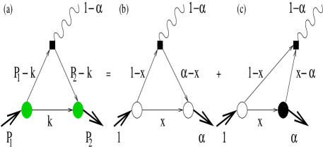
FIG. 2.: The covariant diagram (a) corresponds to the sum of the LF valence diagram (b) defined in $0<x<\alpha$ region and the nonvalence diagram (c) defined in $\alpha<x<1$ region. The large white and black blobs at the meson-quark vertices in (b) and (c) represent the ordinary LF wave function and the nonvalence wave function vertices, respectively. The small black box at the quark-gauge boson vertex indicates the insertion of the relevant Wilson operator.

As shown in Fig. 2, the $q^{+}$$>$0 frame requires not only the particle-number-conserving (valence) Fock state contribution in Fig. 2(b) but also the particle-number-nonconserving (nonvalence) Fock state contribution in Fig. 2(c); i.e. $j^{+}(\alpha_{\pm})=j^{+}_{val}(\alpha_{\pm})+j^{+}_{nv}(\alpha_{\pm})$ in Eq. (52). In our previous works [22, 23], we have developed a new effective treatment of the non-wave-function vertex(black blob in Fig. 2(c)) in the nonvalence diagram arising from the quark-antiquark pair creation/annihilation. Since the detailed procedures for obtaining the effective solution for the non-wave-function vertex have been given in [22, 23], here we briefly present the salient points of our effective method [22, 23] and the final forms of the current matrix elements for both valence and nonvalence diagrams.

The essential feature of our approach is to consider the light-front wave function as the solution of light-front Bethe-Salpeter equation(LFBSE) given by

$$(M^{2}-{\cal M}^{2}_{0})\Psi(x_{i},{\vec{k}}_{i\perp})$$ (53)

$$\;\;=\int[dy][d^{2}{\vec{l}}_{\perp}]{\cal K}(x_{i},{\vec{k}}_{i\perp};y_{j},{\vec{l}}_{j\perp})\Psi(y_{j},{\vec{l}}_{j\perp}),$$ (54)

where ${\cal K}$ is the B-S kernel which in principle includes all the higher Fock-state contributions, ${\cal M}^{2}_{0}=(m^{2}_{1}+{\vec{k}}^{2}_{1\perp})/x_{1}+(m^{2}_{2}+{\vec{k}}^{2}_{2\perp})/x_{2}$, and $\Psi(x_{i},{\vec{k}}_{i\perp})$ is the B-S amplitude. Both the valence(white blob) and nonvalence(black blob) B-S amplitudes are solutions to Eq. (53). For the normal(or valence) B-S amplitude, $x_{1}=x$ and $x_{2}=\alpha-x>0$, while for the nonvalence B-S amplitude, $x_{1}=x$ and $x_{2}=\alpha-x<0$. As illustrated in Figs. 2(b) and (c), the nonvalence B-S amplitude is an analytic continuation of the valence B-S amplitude. In the LFQM the relationship between the B-S amplitudes in the two regions is given by [22, 23]

$$(M^{2}-{\cal M}^{2}_{0})\Psi^{\prime}(x_{i},{\vec{k}}_{i\perp})$$ (55)

$$\;\;=\int[dy][d^{2}{\vec{l}}_{\perp}]{\cal K}(x_{i},{\vec{k}}_{i\perp};y_{j},{\vec{l}}_{j\perp})\Psi(y_{j},{\vec{l}}_{j\perp}),$$ (56)

where $\Psi^{\prime}(x_{i},{\vec{k}}_{i\perp})$ represents the nonvalence B-S amplitude and again the kernel includes in principle all the higher Fock state contributions because all the higher Fock components of the bound-state are ultimately related to the lowest Fock component with the use of the kernel. This is illustrated in Fig. 3.

FIG. 3.: Non-wave-function vertex(black blob) linked to an ordinary LF wave function(white blob).

Equations (53) and (55) are integral equations for which one needs nonperturbative QCD to obtain the kernel. We do not solve for the B-S amplitudes in this work, but a nice feature of Eq. (55) is a natural link between nonvalence B-S amplitude $\Psi^{\prime}$ and the valence one $\Psi$ which enables an application of a light-front CQM even for the calculation of nonvalence contribution in Fig. 2(c). In ($1+1$)-QCD models [35, 36], it is shown that expressions for the nonvalence vertex analogous to our form given in Eq. (55) are obtained. With the iteration procedure given by Eq. (55) in this $q^{+}>0$ frame, we obtain the current matrix element of the nonvalence diagram in terms of light-front vertex function and the gauge boson vertex function. The interested reader may consult Refs. [22, 23] on this subject.

The matrix element of the valence current, $j^{+}_{val}$ in Eq. (52), is given by

$${}j^{+}_{val} = \int^{\alpha}_{0}dx\int d^{2}{\vec{k}}_{\perp}\sqrt{\frac{\partial k^{\prime}_{z}}{\partial x^{\prime}}}\sqrt{\frac{\partial k_{z}}{\partial x}}\phi_{2}(x^{\prime},{\vec{k}}_{\perp})\phi_{1}(x,{\vec{k}}_{\perp})$$ (58)

$$\times\frac{B_{1}B_{2}+{\vec{k}}^{2}_{\perp}}{\sqrt{B_{1}^{2}+\vec{k}^{2}_{\perp}}\sqrt{B_{2}^{2}+\vec{k}^{2}_{\perp}}},$$

where

$$B_{1}=xm_{1}+(1-x)m_{\bar{q}},\;B_{2}=x^{\prime}m_{2}+(1-x^{\prime})m_{\bar{q}},$$ (59)

and $k^{\prime}_{z}=k_{z}(x^{\prime},{\vec{k}}_{\perp})$ in Eq. (38). The matrix element of the nonvalence current, $j^{+}_{nv}$ in Eq. (52), is obtained as

$${}j^{+}_{nv} = \int^{1}_{\alpha}\frac{dx}{x^{\prime}(1-x^{\prime})}\int d^{2}{\vec{k}}_{\perp}\sqrt{\frac{\partial k_{z}}{\partial x}}\chi^{g}(x,{\vec{k}}_{\perp})\phi_{1}(x,{\vec{k}}_{\perp})$$ (62)

$$\times\frac{{\vec{k}}^{2}_{\perp}+B_{1}B_{2}+x(1-x)(1-x^{\prime})(M^{2}_{1}-M^{2}_{0})}{\sqrt{x(1-x)}\tilde{M}_{0}}$$

$$\times\int\widehat{dy}\int d^{2}{\vec{l}}_{\perp}\sqrt{\frac{\partial l_{z}}{\partial y}}\frac{{\cal K}(x,{\vec{k}}_{\perp};y,{\vec{l}}_{\perp})}{\tilde{M^{\prime}}_{0}(y,{\vec{l}_{\perp}})}\phi_{2}(y,{\vec{l}}_{\perp}),$$

where

$$\chi^{g}(x,{\vec{k}}_{\perp})=\frac{1}{\alpha\biggl{[}\frac{q^{2}}{1-\alpha}-\biggl{(}\frac{{\vec{k}}^{2}_{\perp}+m^{2}_{1}}{1-x}+\frac{{\vec{k}}^{2}_{\perp}+m^{2}_{2}}{x-\alpha}\biggr{)}\biggr{]}}$$ (63)

is the light-front vertex function of a gauge boson and $\widehat{dy}=dy/\sqrt{y(1-y)}$. In derivation of Eq. (62) with the “+”-component of the current, we also separate the on-mass shell propagating part(i.e. the term proportional to $({\vec{k}}^{2}_{\perp}+B_{1}B_{2})$) from the instantaneous part(i.e. the term proportional to $x(1-x)(1-x^{\prime})(M^{2}_{1}-M^{2}_{0})$), where the struck quarks ($m_{1}=m_{b}$ and $m_{2}=m_{s}$) are on-mass shell and the spectator quark ($m_{\bar{q}}=m_{u}$) is off-mass shell. Note that the instantaneous contribution exists only for the nonvalence diagram as far as the “$+$”-component of the current is used. As we shall show in the next numerical section, the instantaneous contribution to the weak form factors $F_{\pm}(q^{2})$ for $B\to K$ transition is quite substantial near zero recoil.

Note that Eq. (55) was used to obtain the last term in Eq. (62). While the relevant operator ${\cal K}$ is in general dependent on all internal momenta $(x,{\vec{k}}_{\perp};y,{\vec{l}}_{\perp})$, the integral of ${\cal K}$ over $y$ and ${\vec{l}}_{\perp}$ in Eq. (62) depends only on $x$ and ${\vec{k}}_{\perp}$, which we define

$$G_{BK}(x,{\vec{k}}_{\perp})\equiv\int\widehat{dy}\int d^{2}{\vec{l}}_{\perp}\sqrt{\frac{\partial l_{z}}{\partial y}}\frac{{\cal K}(x,{\vec{k}}_{\perp};y,{\vec{l}}_{\perp})}{\tilde{M^{\prime}}_{0}(y,{\vec{l}_{\perp}})}\phi_{2}(y,{\vec{l}}_{\perp}).$$ (64)

In this work, we approximate $G_{BK}(x,{\vec{k}}_{\perp})$ as a constant which has been tested in our previous works [22, 23] and proved to be a good approximation. As we shall show in the next section, the reliability of this approximation can be checked by examining the frame-independence of our numerical results.

IV Numerical results

In our numerical calculation for the process of $B\to K\ell^{+}\ell^{-}$ transition, we use the linear potential parameters presented in Ref. [21]. Our predictions of the decay constants for $K$ and $B$ were reported [20, 21] as $f_{K}$=161.4 MeV(Exp.= 159.8$\pm$1.4) [20] and $f_{B}=171.4$ MeV [21], respectively. Our model parameters and decay constants are summarized in Table I and compared with experimental data [31] as well as lattice results [37]. Note that in the numerical calculations we take $m_{b}=5.2$ GeV in all formulas except in the Wilson coefficient $C^{\rm eff}_{9}$, where $m_{b}=4.8$ GeV has been commonly used.

FIG. 4.: Analytic solutions of $F_{+}(q^{2})$(thick solid line) and $F_{T}(q^{2})$(thick dashed line) compared with the results(thin lines) obtained from the parametric formula given by Eq. (46) for $B\to K$ transition.

In Fig. 4, we show our analytic($q^{+}=0$ frame) solutions for the weak form factors $F_{+}(q^{2})$(thick solid line) and $F_{T}(q^{2})$(thick dashed line) for $-5\;{\rm GeV}^{2}\leq q^{2}\leq(M_{B}-M_{K})^{2}$. We also include the results obtained from the parametric formula given by Eq. (46) where the thin solid(dashed) line represents $F_{+}(F_{T})$. Our analytic solutions given by Eqs. (42) and (44) are well approximated by Eq. (46) up to $q^{2}\lesssim 15$ GeV² but show some deviations near zero recoil point. We summarize in Table II our numerical results for the weak form factors $F_{+}(q^{2})$ and $F_{T}(q^{2})$ at $q^{2}=0$ and the parameters $\sigma_{i}$ defined in Eq. (46) and compare with other theoretical results [7, 9, 13, 29]. As one can see from Table II, our results for the $F_{+}(q^{2})$ and $F_{T}(q^{2})$ in $q^{2}\to 0$ limit are quite comparable with other theoretical results. As other theoretical schemes predicted, our results also show $F_{+}(0)(=0.348)\simeq-F_{T}(0)(=-0.324)$.

FIG. 5.: Effective solution of $F_{+}(q^{2})$(thin solid line) for $B\to K$ transition. The line code is in the figure.

For the analysis of heavy $\tau$ decay process, the weak form factor $F_{-}(q^{2})$(or equivalently $F_{0}(q^{2})$) is necessary for the calculations of the decay rate and the LPA and we obtain it using our effective method [22, 23] in $q^{+}>0$ frame as described in Sec. III(B). In Fig. 5, we show our effective($q^{+}>0$ frame) solution of $F_{+}(q^{2})$ (thin solid line) with a constant $G_{BK}=3.9$ fixed by the normalization of $F_{+}(q^{2})$ in the $q^{+}=0$ frame (thick solid line) at $q^{2}=0$ limit. As one can see in Fig. 5, our effective solution of $F_{+}(q^{2})$(thin solid line) is very close to the analytic one(thick solid line) for the entire kinematic region. It justifies the reliability of our constant approximation $G_{BK}$ of the kernel ${\cal K}$. For comparison, we also show the valence(dotted line) and the instantaneous(dot-dashed line) contributions to $F_{+}(q^{2})$ in the $q^{+}>0$ frame. Although the valence contribution dominates over the nonvalence one for $q^{2}\lesssim 10$ GeV², the nonvalence (especially the instantaneous) contribution is not negligible for $q^{2}\gtrsim 10$ GeV².

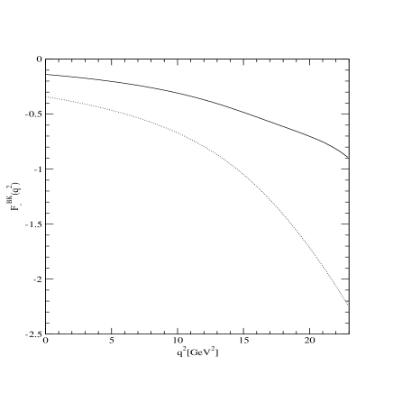
FIG. 6.: Effective solutions(solid line) of $F_{0}(q^{2})$ and $F_{-}(q^{2})$ compared with the valence contributions(dotted line) for $B\to K$ transition.

Using the same constant operator $G_{BK}=3.9$, we are now able to calculate the scalar form factors $F_{0}(q^{2})$ and $F_{-}(q^{2})$ in $q^{+}>0$ frames and the results are shown in Fig. 6(solid line). As in the case of $F_{+}(q^{2})$ in Fig. 5, we also include the valence contributions(dotted line) to both $F_{0}(q^{2})$ and $F_{-}(q^{2})$ and the instantaneous contribution(dot-dashed line) to $F_{0}(q^{2})$. It is very interesting to note especially from $F_{-}(q^{2})$ that the nonvalence contribution, i.e. the difference between solid and dotted lines, is very substantial even at the maximum recoil point($q^{2}=0$) and is growing as $q^{2}$ increases. As a reference, our numerical results for $F_{-}$ obtained from our effective(valence) solution at maximum- and zero-recoil limits are $F_{-}(0)=-0.14(-0.34)$ and $F_{-}(q^{2}_{\rm max})=-0.9(-2.23)$, respectively. Our result for $F_{-}(q^{2})$ presented in Fig. 6 agrees very well with the light cone QCD sum rule (LCSR) result for $F_{-}(q^{2})$ by Aliev et al. [15](See their Fig.1(b)). Similarly, our effective solution for $F_{0}(q^{2})$ is in a close agreement with the LCSR results given by Ball [13] and Ali et al. [16]. Our effective solution of $F_{0}(q^{2})$ as well as the analytic solutions of $F_{+}(q^{2})$ and $F_{T}(q^{2})$ shown in Fig. 4 will be used for the calculations of the branching ratios and the longitudinal lepton polarization asymmetries. We shall also discuss how we take the effect of the vector meson dominance(VMD) into account at the end of this section.

FIG. 7.: The branching ratios for $B\to K\ell^{+}\ell^{-}$($\ell=e,\mu$)(a) and $B\to K\tau^{+}\tau^{-}$(b) transitions. The thick(thin) solid line represents the result with(without) LD contribution to $C^{\rm eff}_{9}$ in Eq. (10). The dotted line in (b) represents the $F_{0}(q^{2})$ contribution to the total branching ratio of $\tau$ decay.

We now show our results for the differential branching ratios for $B\to K\ell^{+}\ell^{-}(\ell=e,\mu)$ in Fig. 7(a) and $B\to K\tau^{+}\tau^{-}$ in Fig. 7(b), respectively. The thick(thin) solid line represents the result with(without) the LD contribution($Y_{LD}(\hat{s})$) to $C^{\rm eff}_{9}$ given by Eq. (10). In plotting Figs. 7(a) and (b), we set $m_{\ell}=0$ and $m_{\tau}$=1.777 GeV, respectively. As one can see the pole contributions clearly overwhelm the branching ratio near $J/\psi(1S)$ and $\psi^{\prime}(2S)$ peaks, however, suitable $\ell^{+}\ell^{-}$ invariant mass cuts can separate the LD contribution from the SD one away from these peaks. This divides the spectrum into two distinct regions [24, 38]: (i) low-dilepton mass, $4m^{2}_{\ell}\leq q^{2}\leq M^{2}_{J/\psi}-\delta$, and (ii) high-dilepton mass, $M^{2}_{\psi^{\prime}}+\delta\leq q^{2}\leq q^{2}_{\rm max}$, where $\delta$ is to be matched to an experimental cut. The branching ratios with[without] the pole(i.e. LD) contributions for $B\to K\ell^{+}\ell^{-}$ are presented in Table III for low(second column), high(third column), and total(4th column) dilepton mass regions of $q^{2}$. Although the contribution of scalar form factor $F_{0}(q^{2})$ to massless lepton decay is negligible(zero for $m_{\ell}=0$), its contribution to $\tau$-decay as shown in Fig. 7(b)(dotted line) is very substantial, e.g. $\sim 75\%$ contribution to the total(nonresonant) decay rate in our model calculation. Thus, the reliable calculation of $F_{0}(q^{2})$ is absolutely necessary and our effective method of calculating the nonvalence diagram seems very useful.

It is worthwhile to compare our results for the branching ratios with other light-front quark models[8, 10]. While the authors in Ref. [8] used the simple parametric formula, Eq. (46), to obtain $F_{+}$ and $F_{T}$ and the heavy quark symmetry(HQS) to extract $F_{-}$, the authors in Ref. [10] used the dispersion representation through the (Gaussian) wave functions of the initial and final mesons and then analytically continue the form factors from the spacelike region to the timelike region. The common aspect in these models is to have the same form factors $F_{+}$ and $F_{T}$, which are free from the zero-mode contribution, not in the timelike region but in the spacelike region as far as the same model parameters are used. Indeed our method of analytic continuation of the form factors $F_{+}$ and $F_{T}$ is equivalent to that of Ref. [10]. However, the difference is in the calculation of $F_{-}$, which is not immune to the zero-mode contribution. The zero-mode contribution must be properly taken into account for the calculation of $F_{-}$. Thus, it is not quite surprising to note that although our branching ratio(see Fig. 7(a)) for the massless lepton $(\ell=e,\mu$) decay is not much different from the results in Ref. [8](see their Fig. 1(a)) and Ref. [10](see their Fig. 3(a)), our branching ratio(see Fig. 7(b)) for the $\tau$ decay is quite different from the results in Ref. [8](see their Fig. 1(b)) and Ref. [10](see their Fig. 3(c)).

Our numerical results for the non-resonant branching ratios(assuming $|V_{tb}|\simeq 1$) are $4.96\times 10^{-7}|V_{ts}/V_{cb}|^{2}$ for $B\to K\ell^{+}\ell^{-}$ ($\ell=e,\mu$) and $1.27\times 10^{-7}|V_{ts}/V_{cb}|^{2}$ for $B\to K\tau^{+}\tau^{-}$, respectively. While the CLEO Collaboration [1] reported the branching ratio ${\rm Br}(B\to Ke^{+}e^{-})<1.7\times 10^{-6}$, the Belle Collaboration(K. Abe et al.) [1] reported ${\rm Br}(B\to Ke^{+}e^{-})<1.2\times 10^{-6}$ and ${\rm Br}(B\to K\mu^{+}\mu^{-})=(0.99^{+0.39+0.13}_{-0.32-0.15})\times 10^{-6}$, respectively. Our non-resonant results for the branching ratios of $B\to K\ell^{+}\ell^{-}$ is summarized in Table IV and compared with experimental data as well as other theoretical predictions within the SM.

The exclusive $B\to K\tau^{+}\tau^{-}$ has been computed via the heavy meson chiral perturbation theory by Du et al. [18], where the branching ratio of the exclusive decay was found to be about $50-60\%$ of the inclusive one. Although calculations of exclusive decay rates are inherently model dependent, chiral perturbation theory is known to be reliable at energy scales smaller than the typical scale of chiral symmetry breaking, $\Lambda_{\rm CSB}\simeq 4\pi f_{\pi}/\sqrt{2}$. In $B\to K\tau^{+}\tau^{-}$, the maximum energy of the $K$-meson in the $B$ rest frame is $(M^{2}_{B}+M^{2}_{K}-4m^{2}_{\tau})/2M_{B}\sim 1.5$ GeV, which places most of the available phase space around the scale $\Lambda_{\rm CSB}$ [18, 24]. From the above argument and our exclusive $\tau$ branching fraction, we can estimate the branching ratio of inclusive $B\to X_{s}\tau^{+}\tau^{-}$ as $(2.12-2.54)\times 10^{-7}|V_{ts}/V_{cb}|^{2}$ which is quite comparable to the prediction given by Hewett [24] where ${\rm BR}(B\to X_{s}\tau^{+}\tau^{-})=2.5\times 10^{-7}$ was obtained.

In Figs. 8(a) and (b), we show the longitudinal lepton polarization asymmetries for $B\to K\mu^{+}\mu^{-}$ and $B\to K\tau^{+}\tau^{-}$ as a function of $\hat{s}$, respectively, and with (thick solid line) and without (thin solid line) LD contributions. For the $B\to K\mu^{+}\mu^{-}$ case, we use the physical muon mass, $m_{\mu}$=105 MeV. In both figures, the longitudinal lepton polarization asymmetries become zero at the end point regions of $\hat{s}$. Our numerical values of $P_{L}$ without LD contributions and away from the end point regions are $-0.97<P_{L}<-0.98$ in $0.3<\hat{s}<0.6$ region for $B\to K\mu^{+}\mu^{-}$ and $-0.15<P_{L}<-0.18$ in $0.5<\hat{s}<0.7$ region for $B\to K\tau^{+}\tau^{-}$, respectively. In fact, the $P_{L}$ for the muon decay is insensitive to the form factors, e.g. our $P_{L}\simeq-0.98$(away from the end points region) is well approximated by [11]

$$P_{L}\simeq 2\frac{C_{10}{\rm Re}C^{\rm eff}_{9}}{|C^{\rm eff}_{9}|^{2}+|C_{10}|^{2}}\simeq-1,$$ (65)

in the limit of $C_{7}\to 0$ from Eq. (26). It also shows that the $P_{L}$ for the $\mu$ dilepton channel is insensitive to the little variation of $C_{7}$ as expected. On the other hand, the LPA for the $\tau$ dilepton channel is sensitive to the form factors. In other words, as in the case of branching ratios, although our result of the LPA for the muon decay is not much different from the results in Ref. [8](see their Fig. 2(a)) and Ref [10](see their Fig. 5(a)), the result for the tau decay is quite different from the results in Ref. [8](see their Fig. 2(b)) and Ref [10](see their Fig. 5(c)).

FIG. 8.: The longitudinal lepton polarization asymmetries $P_{L}(\hat{s})$ for $B\to K\ell^{+}\ell^{-}$(a) and $B\to K\tau^{+}\tau^{-}$(b) transitions. The same line code is used as in Fig. 7.

Comparing our results for the weak form factors with other phenomenological models, one may find that there is in general a good agreement for small and intermediate $q^{2}$ region. Nevertheless, there are some differences for large $q^{2}$ region where vector mesons are expected to dominate(VMD) especially for $F_{+}(q^{2})$. For example, both results of the LCSR in [13, 39] and our LFQM analyses show that the direct solution for $F_{+}(q^{2})$ is well approximated by Eq. (46) up to $q^{2}\lesssim 15$ GeV². However, the large momentum behavior of $F_{+}(q^{2})$(as well as $F_{T}(q^{2})$) is somewhat different since our model does not include the VMD effect.

Following the same method used in recent LCSR analysis [39], we use the VMD formula(i.e. $B^{*}$-pole with $M_{B^{*}}=5.325$ GeV) given by

$$F^{\rm VMD}_{+}(q^{2})=\frac{c}{1-q^{2}/M^{2}_{B^{*}}}$$ (66)

at large $q^{2}$ region and match the parametric formula $F_{+}(q^{2})$ in Eq. (46) by the following constraint [39]

$$F^{\rm VMD}_{+}(q^{2})=F_{+}(q^{2})\;{\rm in}\;{\rm Eq.~{}(\ref{Pole})},$$ (67)

$$\frac{d}{dq^{2}}F^{\rm VMD}_{+}(q^{2})=\frac{d}{dq^{2}}F_{+}(q^{2})\;{\rm in}\;{\rm Eq.~{}(\ref{Pole})},$$ (68)

to make both parametrizations smooth connection at a transition point $q^{2}=q^{2}_{0}$, where $c$ is fixed at $q^{2}=q^{2}_{0}$ in Eq. (67). We should note that the $F_{+}(q^{2})$ in Eq. (46) is almost equivalent to our LFQM prediction $F^{\rm LFQM}_{+}(q^{2})$ up to $q^{2}\lesssim 15$ GeV² and the transition point $q^{2}_{0}$ is expected to be at $q^{2}\sim 15$ GeV²(see also Ref. [39]) in order to make interpolation between $F^{\rm LFQM}(q^{2}\leq q^{2}_{0})$ and $F^{\rm VMD}(q^{2}\geq q^{2}_{0})$ more sense. In our case for $B\to K$ transition, we obtain $(c,q^{2}_{0})$=(0.388, 14.38 GeV²) for $F^{\rm BK}_{+}(q^{2})$. For the tensor form factor, we get $(c,q^{2}_{0})$=($-0.358$, 14.23 GeV²) for $F_{T}(q^{2})$.

It is necessary to discuss the exclusive $B\to\pi\ell\nu_{\ell}$ process in that the constant $c$ has a direct physical implication for $B\to\pi\ell\nu_{\ell}$ process, i.e. it is related to the physical couplings as [39, 41, 42]

$$c=\frac{f_{B^{*}}g_{B^{*}B\pi}}{2M_{B^{*}}}$$ (69)

where $f_{B^{*}}$ is the decay constant of the $B^{*}$ meson defined by $\langle 0|\bar{b}\gamma^{\mu}u|B^{*}\rangle=M_{B^{*}}f_{B^{*}}\epsilon^{\mu}$ and $g_{B^{*}B\pi}$ is the (axial-current) coupling defined by $\langle B^{0}(P)\pi^{+}(q)|B^{*+}(P+q)\rangle=g_{BB^{*}\pi}(q\cdot\epsilon)$ and can be extracted from soft pion $q^{2}\to 0$ limit in the heavy meson chiral perturbation theory [43, 44]. In the limit where the heavy quark mass $m_{Q}(Q=c,b)$ goes to infinity there are flavor-independent relations between coupling constants

$$g=\frac{f_{\pi}}{2M_{D}}g_{D^{*}D\pi}=\frac{f_{\pi}}{2M_{B}}g_{B^{*}B\pi},$$ (70)

where $f_{\pi}=131$ MeV and the coupling constant $g$ appears in the interaction Lagrangian of the effective meson field theory [17, 43, 44].

In our numerical calculation of $c$ for the exclusive $B\to\pi e\nu_{e}$ process, we obtain ($c,q^{2}_{0}$)=(0.312,15.12 GeV²) from Eq. (67) and $(\sigma_{1},\sigma_{2})=(4.75\times 10^{-2},5.50\times 10^{-4})$ in Eq. (46), which was obtained in our previous analysis [45]. Since we also obtained the $B^{*}$ meson decay constant as $f_{B^{*}}=185.8$ MeV [45], we can now extract the coupling constant of the $B^{*}$ to $B\pi$-pair and the result is $g_{B^{*}B\pi^{+}}=17.88$ and $g$=0.23 while the recent fit [46] to the experimental data gives two possible solutions, $g=0.27^{+0.04+0.05}_{-0.02-0.02}$ or $g=0.76^{+0.03+0.2}_{-0.03-0.1}$. We acknowledge the remark in [46] that for the $B\to\pi\ell\nu_{\ell}$ form factors with $E_{\pi}<2m_{\pi}$, analytic bounds combined with chiral perturbation theory give $gf_{B}\lesssim 50$ MeV [47]. That means while the solution $g=0.27$ gives $f_{B}\lesssim 190$ MeV, $g=0.76$ gives $f_{B}\lesssim 66$ MeV, which is roughly a factor of three smaller than lattice QCD result [37],i.e. $f^{\rm Lat.}_{B}=200\pm 30$ MeV. Note that our LFQM prediction is given by $f^{\rm LFQM}_{B}=171.4$ MeV. As a reference, other theoretical calculations for $g$ are $0.2-0.4$ for the QCD sum rules, $1/3-0.6$ for the quark models and 0.42(4)(8) for the lattice calculation(see Ref. [48] for the survey of $g$ values obtained from different models).

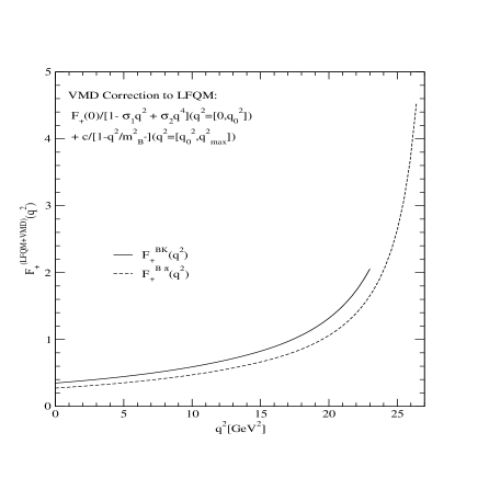
FIG. 9.: VMD corrections to the LFQM predctions for $F^{BK}_{+}(q^{2})$(solid line) and $F^{B\pi}_{+}(q^{2})$(dashed line), i.e. $F_{+}(q^{2})=F^{\rm LFQM}_{+}(q^{2}\leq q^{2}_{0})+F^{\rm VMD}_{+}(q^{2}\geq q^{2}_{0})$.

In Fig. 9, we show the VMD corrections to both $F^{BK}_{+}(q^{2})$(solid line) and $F^{B\pi}_{+}(q^{2})$(dashed line), i.e. $F_{+}(q^{2})=F^{\rm LFQM}_{+}(q^{2}\leq q^{2}_{0})+F^{\rm VMD}_{+}(q^{2}\geq q^{2}_{0})$. Comparing Fig. 4[Fig. 3 in [21]] and Fig. 9, we find the enhancement of $F^{BK}_{+}(q^{2})[F^{B\pi}_{+}(q^{2})]$ at $q^{2}=q^{2}_{\rm max}$ by around $40[70]\%$. Our result for $F^{B\pi}_{+}(q^{2})$ including the VMD correction are quite comparable with that obtained from QCD sum rules in Ref. [39] where the authors used the same method to enhance $F^{B\pi}_{+}(q^{2})$. Our result for $F^{BK}_{+}(q^{2})$ in Fig. 9 is also comparable with those of Refs. [13, 16]. However, the branching ratio for $B\to K\ell^{+}\ell^{-}$($\ell=e,\mu$) increases less than $2\%$ by including the VMD effect. It is not surprising to note that the large enhancement of the weak form factors near the zero-recoil($q^{2}=q^{2}_{\rm max}$) region does not affect the differential decay rate very much, since the phase space of the large $q^{2}$ region is highly suppressed in Eq. (20).

V Summary and Conclusion

In this work, we investigated the rare exclusive semilpetonic $B\to K\ell^{+}\ell^{-}$ ($\ell=e,\mu$ and $\tau$) decays within the SM, using our LFQM which has been tested extensively in spacelike processes [20, 23] as well as in the timelike exclusive semileptonice decays of pseudoscalar mesons [21, 22]. The form factors $F_{+}(q^{2})$ and $F_{T}(q^{2})$ are obtained in the $q^{+}=0$ frame ($q^{2}<0$) and then analytically continued to the timelike region by changing $q_{\perp}$ to $iq_{\perp}$ in the form factors. The form factor $F_{-}(q^{2})$ is obtained from our effective treatment of the nonvalence contribution in addition to the valence one in $q^{+}>0$ frames ($q^{2}>0$) based on the B-S formalism. The covariance (i.e. frame-independence) of our model has been checked by comparison of $F_{+}(q^{2})$ obtained from both $q^{+}=0$ and $q^{+}>0$ frames. Our numerical results for the form factors are comparable with other theoretical calculations as shown in Table II. Using the solutions of $F_{+}$ and $F_{T}$ obtained from $q^{+}=0$ frame and $F_{-}$ obtained from $q^{+}>0$ frame, we calculate the branching ratios and the longitudinal lepton polarization asymmetries for $B\to K\ell^{+}\ell^{-}$ including both short- and long-distance contributions from QCD Wilson coefficients. Our numerical results for the non-resonant branching ratios are in the order of $10^{-7}$, which are consistent with many other theoretical predictions as shown in Table IV. Of particular interest, we were able to estimate the inclusive branching ratio for $B\to X_{s}\tau^{+}\tau^{-}$ as ${\rm BR}(B\to X_{s}\tau^{+}\tau^{-})\sim(2.12-2.54)\times 10^{-7}|V_{ts}/V_{cb}|^{2}$ with the help of chiral perturbation theory [18]. For the LPA as a parity-violating observable, we find that the LPA for the $\tau$ channel is sensitive to the form factors while the LPA for the $\mu$ channel is insensitve to the model for the hadronic form factors. Thus, the experimental data of the LPA for $\tau$ decay would provide a useful guidance for the model building of hadrons and make a definitive test on existing models.

REFERENCES

- [1] K. Abe et al., Belle Collaboration, hep-ex/0107072;hep-ex/0109026; S. Anderson et al., CLEO Collaboration, hep-ex/0106060; B. Aubert et al., BaBar Collaboration, Phys. Rev. Lett. 86, 2515 (2001)[hep-ex/0102030]; A. Abashian et al., Belle Collaboration, Phys. Rev. Lett. 86, 2509 (2001)[hep-ex/0102018].
- [2] B. Grinstein, M. B. Wise and M. J. Savage, Nucl. Phys. B 319, 271 (1989).
- [3] A. J. Buras and M. Mnz, Phys. Rev. D 52, 186 (1995).
- [4] M. Misiak, Nucl. Phys. B 393, 23 (1993); . 439, 461(E) (1995).
- [5] T. Inami and C. S. Lim, Prog. Theor. Phys. 65, 297 (1981); G. Buchalla and A. J. Buras, Nucl. Phys. B 400, 225 (1993).
- [6] A. Ali, T. Mannel and T. Morozumi, Phys. Lett. B 273, 505 (1991); A. Ali, Acta Phys. Pol. B 27, 3529 (1996).
- [7] W. Jaus and D. Wyler, Phys. Rev. D 41, 3405 (1990); C. Greub, A. Ioannissian and D. Wyler, Phys. Lett. B 346, 149 (1995).
- [8] C. Q. Geng and C. P. Kao, Phys. Rev. D 54, 5636 (1996).
- [9] D. Melikhov, N. Nikitin, and S. Simula, Phys. Lett. B 410, 290 (1997); 430, 332 (1998).
- [10] D. Melikhov and N. Nikitin, Phys. Rev. D 57, 6814 (1998).
- [11] W. Roberts, Phys. Rev. D 54, 863 (1996); G. Burdman, Phys. Rev. D 52, 6400 (1995).
- [12] P. Colangelo et al., Phys. Rev. D 53, 3672 (1996); Phys. Lett. B 395, 339 (1997).
- [13] P. Ball, JHEP 9809, 005 (1998)[hep-ph/9802394].
- [14] P. Ball and V. M. Braun, Phys. Rev. D 58, 094016 (1998).
- [15] T. M. Aliev et al., Phys. Lett. B 400, 194 (1997).
- [16] A. Ali et al., Phys. Rev. D 61, 074024 (2000).
- [17] R. Casalbuoni et al., Phys. Rep. 281, 145 (1997).
- [18] D. Du, C. Liu, and D. Zhang, Phys. Lett. B 317, 179 (1993).
- [19] S. J. Brodsky, H. -C. Pauli, and S. S. Pinsky, Phys. Rep. 301, 299 (1998).
- [20] H. -M. Choi and C. -R. Ji, Phys. Rev. D 59, 074015 (1999).
- [21] H.-M. Choi and C. -R. Ji, Phys. Lett. B 460, 461 (1999); Phys. Rev. D 59, 034001 (1998).
- [22] C. -R. Ji and H. -M. Choi, Phys. Lett. B 513, 330 (2001) ; C. -R. Ji and H. -M. Choi, eConf C010430:T23 (2001) [hep-ph/0105248].
- [23] H. -M. Choi, C. -R. Ji, and L. S. Kisslinger, Phys. Rev. D 64, 093006 (2001).
- [24] J. L. Hewett, Phys. Rev. D 53, 4964 (1996); F. Krger and L. M. Sehgal, Phys. Lett. B 380, 199 (1996).
- [25] T. M. Aliev et al., Phys. Rev. D 64, 055007 (2001); S. Fukae, C. S. Kim and T. Yoshikawa, Phys. Rev. D 61, 074015 (2000); T. M. Aliev, K. Cakmak, M. Savci, Nucl. Phys. B 607, 305 (2001).
- [26] H. -M. Choi and C. -R. Ji, Nucl. Phys. A 679, 735 (2001).
- [27] H. -M. Choi and C. -R. Ji, Phys. Rev. D 58, 071901 (1998).
- [28] C. S. Kim, T. Morozumi, and A. I. Sanda, Phys. Rev. D 56, 7240 (1997).
- [29] T. M. Aliev, C. S. Kim, and M. Savci, Phys. Lett. B 441, 410 (1998).
- [30] Z. Ligeti and M. B. Wise, Phys. Rev. D 53, 4937 (1996).
- [31] D. E. Groom et al., Eur. Phys. J. C 15, 1 (2000).
- [32] M. Neubert and B. Stech, Heavy Flavors II 294-344, edited by A. J. Buras and M. Lindner, World Scientific, Singapore [hep-ph/9705292].
- [33] M. Jeabek and J. H. Khn, Nucl. Phys. B 320, 20 (1989).
- [34] N. G. Deshpande and J. Trampetic, Phys. Rev. Lett. 60, 2583 (1988).
- [35] M. B. Einhorn, Phys. Rev. D 14, 3451 (1976).
- [36] M. Burkardt, Phys. Rev. D 62, 094003 (2000).
- [37] C. Bernard, Nucl. Phys. Proc. Suppl. 94, 159 (2001).
- [38] A. Ali, G. F. Guidice, and T. Mannel, Z. Phys. C 67, 417 (1995).
- [39] P. Ball and R. Zwicky, JHEP 0110, 019 (2001)[hep-ph/0110115].
- [40] W. Jaus, Phys. Rev. D 53, 1349 (1996).
- [41] V. M. Belyaev, V. M. Braun, A. Khodjamirian, R. Rückl, Phys. Rev. D 51, 6177 (1995).
- [42] A. Khodjamirian, R. Rückl, S. Weinzierl, and O. Yakovlev, Phys. Lett. B 457, 245 (1999).
- [43] M. B. Wise, Phys. Rev. D 45, 2188 (1992).
- [44] G. Burdman and J. F. Donoghue, Phys. Lett. B 280, 287 (1992); L. Wolfenstein, Phys. Lett. B 291, 177 (1992); T. M. Yan et al. Phys. Rev. D 46, 1148 (1992).
- [45] H.-M. Choi, Ph.D. thesis [hep-ph/9911271]
- [46] I. W. Stewart, Nucl. Phys. B 529, 62 (1998).
- [47] C. G. Boyd, et al., Phys. Rev. Lett. 74, 4603 (1995).
- [48] D. Becirevic and A. L. Yaouanc, JHEP 9903, 021 (1999)[hep-ph/9901431].