Nonequilibrium Phenomena in Quantum Field Theory:
From Linear Response to Dynamical Renormalization Group

by
Shang-Yung Wang
BS, National Taiwan University, Taiwan, 1991
MS, National Tsing Hua University, Taiwan, 1993

Submitted to the Graduate Faculty of
Arts and Sciences in partial fulfillment
of the requirements for the degree of
Doctor of Philosophy

University of Pittsburgh
2001

UNIVERSITY OF PITTSBURGH

FACULTY OF ARTS AND SCIENCES
This dissertation was presented
by
Shang-Yung Wang

It was defended on
September 28, 2001

and approved by
Richard Holman

David Jasnow

Vittorio Paolone

David Snoke

Frank Tabakin

Daniel Boyanovsky

Committee chairperson

This thesis is devoted to studying aspects of real-time nonequilibrium dynamics in quantum field theory by implementing an initial value formulation of quantum field theory. The main focus is on the linear relaxation of mean fields and quantum kinetics in nonequilibrium multiparticle quantum systems with potential applications to ultrarelativistic heavy ion collisions, cosmological phase transitions and condensed matter systems. We first study the damping of fermion mean fields in a fermion-scalar plasma with a view towards understanding baryon transport phenomena during electroweak baryogenesis. We obtain a fully renormalized, retarded and causal equation of motion that describes the relaxation of the mean field towards equilibrium and allows an unambiguous identification of a novel damping mechanism and the corresponding damping rate. Secondly, we apply and extend the renormalization group method to study nonequilibrium dynamics in a self-interacting scalar theory, the $O(4)$ linear sigma model and a hot QED plasma, with the goals of constructing a quantum kinetic description that goes beyond usual Boltzmann kinetics and understanding anomalous (nonexponential) relaxation associated with infrared phenomena. Remarkably, within this framework the quantum kinetic equations and equations of motion for mean fields have the interpretation as the dynamical renormalization group equation which describes the dynamical evolution of a multiparticle system that is insensitive to microscopic details. By solving these equations, we effectively integrate out fast motion dynamics, and are left with an effective theory for slow motion dynamics. As a by-product, the issue of pinch singularities in nonequilibrium quantum field theory is resolved naturally in real time from a quantum kinetic point of view. The final part of this thesis presents a real-time kinetic analysis of direct photon production from a quark-gluon plasma created in ultrarelativistic heavy ion collisions. We show that the direct photon yield is significantly enhanced by the lowest order energy-nonconserving processes originated in the transient lifetime of the quark-gluon plasma. In particular, transverse momentum distribution of direct photons, which features a power law spectrum in the experimentally relevant regime, is proposed as a nonequilibrium signature of the quark-gluon plasma.

List of Publications

Parts of this thesis are based on the following publications, which I published with collaborators during the period of this work.

1. D. Boyanovsky, H.J. de Vega, D.-S. Lee, Y.J. Ng and S.-Y. Wang, Fermion Damping in a Fermion-Scalar Plasma, Phys. Rev. D 59, 105001 (1999).

2. S.-Y. Wang, D. Boyanovsky, H.J. de Vega, D.-S. Lee, and Y.J. Ng, Damping Rates and Mean Free Paths of Soft Fermion Collective Excitations in a Hot Fermion-Gauge-Scalar Theory, Phys. Rev. D 61, 065004 (2000).

3. D. Boyanovsky, H.J. de Vega, and S.-Y. Wang, Dynamical Renormalization Group Approach to Quantum Kinetics in Scalar and Gauge Theories, Phys. Rev. D 61, 065006 (2000).

4. S.-Y. Wang, D. Boyanovsky, H.J. de Vega, and D.-S. Lee, Real-time Nonequilibrium Dynamics in Hot QED Plasmas: Dynamical Renormalization Group Approach, Phys. Rev. D 62, 105026 (2000).

5. S.-Y. Wang and D. Boyanovsky, Enhanced Photon Production from Quark-Gluon Plasma: Finite-Lifetime Effect, Phys. Rev. D 63, 051702(R) (2001).

6. S.-Y. Wang, D. Boyanovsky, and K.-W. Ng, Direct Photons: A Nonequilibrium Signal of the Expanding Quark-Gluon Plasma, hep-ph/0101251 (to appear in Nucl. Phys. A).

Table of Contents

1. 1 Introduction
   1. 1.1 Motivation
   2. 1.2 New Developments in this Thesis
   3. 1.3 Outline of the Thesis
2. 2 Nonequilibrium Quantum Field Theory
   1. 2.1 Closed-Time-Path Formalism
   2. 2.2 Initial Value Problems in Quantum Field Theory
      1. 2.2.1 Linear relaxation of mean fields
      2. 2.2.2 Quantum kinetic theory
3. 3 Fermion Damping in a Fermion-Scalar Plasma
   1. 3.1 Introduction
   2. 3.2 Effective Dirac Equation in the Medium
      1. 3.2.1 Renormalization
      2. 3.2.2 Structure of the self-energy and damping processes
   3. 3.3 Real-Time Evolution of Mean Fields
      1. 3.3.1 Complex poles or resonances
      2. 3.3.2 Scalar decay implies fermion damping
      3. 3.3.3 All-order expression for the damping rate
   4. 3.4 Kinetics of Fermion Relaxation
   5. 3.5 Conclusions
4. 4 Dynamical Renormalization Group Approach to Quantum Kinetics
   1. 4.1 Introduction
   2. 4.2 Self-Interacting Scalar Theory
      1. 4.2.1 Quantum kinetic equation for quasiparticles
      2. 4.2.2 Dynamical renormalization group equation
   3. 4.3 Comparison to the Euclidean Renormalization Group
   4. 4.4 Application: $O(4)$ Linear Sigma Model
      1. 4.4.1 Quantum kinetics of cool pions and sigma mesons
      2. 4.4.2 Relaxation rate for pions and sigma mesons
      3. 4.4.3 Threshold singularities and crossover in relaxation
   5. 4.5 Pinch Singularities and their Resolution
   6. 4.6 Conclusions
5. 5 Nonequilibrium Dynamics in a QED Plasma at High Temperature
   1. 5.1 Introduction
   2. 5.2 Photons Out of Equilibrium
      1. 5.2.1 Relaxation of the gauge mean field
      2. 5.2.2 Quantum kinetics of photons
   3. 5.3 Hard Fermions Out of Equilibrium
      1. 5.3.1 Relaxation of the fermion mean field
      2. 5.3.2 Quantum kinetics of fermion quasiparticles
   4. 5.4 Conclusions
6. 6 Direct Photon Production from the Quark-Gluon Plasma
   1. 6.1 Introduction
   2. 6.2 $S$-matrix Approach and its Shortcomings
   3. 6.3 Bjorken’s Hydrodynamical Model
   4. 6.4 Real-Time Kinetic Approach
      1. 6.4.1 Nonexpanding QGP
      2. 6.4.2 Longitudinally expanding QGP
      3. 6.4.3 Numerical analysis: central collisions at RHIC and LHC energies
   5. 6.5 Conclusions
7. 7 Summary
8. A Renormalization Group and Asymptotic Analysis
9. Bibliography

List of Figures

1. 2.1 The contour along the time axis used to evaluate the generating functional for nonequilibrium Green’s functions.
2. 3.1 The analytic structure of the fermion propagator $S(s,\mathbf{k})$ and the complex contour used for evaluating the mean field $\psi(\mathbf{k},t)$ for (a) $m<2M$ and (b) $m>2M$.
3. 3.2 The fermion damping rate plotted as a function of the momentum for $m/M=4$ and $T/M=150$, 100, and 50.
4. 3.3 The fermion damping rate plotted as a function of the momentum for $m/M=800$ and $T/M=1000$, 800, and 600.
5. 4.1 The Feynman diagrams that contribute to the quantum kinetic equation for a self-interacting scalar theory up to two-loop order.
6. 4.2 The Feynman diagrams that contribute to the quantum kinetic equation for the pion distribution function at one-loop order.
7. 4.3 The Feynman diagrams that contribute to the quantum kinetic equation for the sigma meson distribution function at one-loop order.
8. 5.1 The function $\beta_{T}(\omega,k)/\omega$ plotted as a function of $\omega$ for ultrasoft photons.
9. 5.2 The function $\beta_{T}(\omega,k)/\omega$ plotted as a function of $\omega$ for semihard photons.
10. 6.1 The Feynman diagrams that contribute to the invariant photon production rate from the QGP.
11. 6.2 The ratio of the nonequilibrium and equilibrium hard photon yields plotted as a function of time for $\alpha=1/137$, $\alpha_{s}=0.4$ and $T=200$ MeV.
12. 6.3 The function ${\cal R}_{\rm HTL}(\omega)$ plotted in the limit $E\gg T$.
13. 6.4 Comparison of various contributions to the direct photon yield from a QGP of temperature $T=200$ MeV and lifetime $t=10$ fm/$c$.
14. 6.5 Comparison of nonequilibrium and equilibrium photon yields at midrapidity from a longitudinally expanding QGP at RHIC energies.
15. 6.6 Rapidity distribution of the nonequilibrium photon yield at $p_{T}=1$, 2, and 3 GeV for a longitudinal expanding QGP at RHIC energies.
16. 6.7 Comparison of nonequilibrium and equilibrium photon yields at midrapidity from a longitudinally expanding QGP at LHC energies.

Chapter 1 Introduction

1.1 Motivation

The theoretical study of nonequilibrium dynamics in quantum multiparticle systems dates back to 1961 when Schwinger published a pioneering paper, Brownian Motion of a Quantum Oscillator [1]. Conventional applications of quantum theory are restricted mainly to calculating transition matrices for scattering processes. In his 1961 paper Schwinger showed, for the first time, how quantum theory can be formulated to study initial value problems associated with the dynamical evolution of nonequilibrium quantum systems.

Over the past two decades, nonequilibrium dynamics in quantum field theory has attracted a great deal of interest as new experimental techniques in particle and condensed matter physics continue to probe novel nonequilibrium quantum phenomena that require field-theoretical descriptions. Specific examples of current theoretical interest involving nonequilibrium dynamics of quantum fields include, just to name a few, inflationary dynamics in the early Universe, electroweak baryogenesis, the chiral phase transition and quark-gluon plasma in ultrarelativistic heavy ion collisions, dynamics of phase transition in Bose-Einstein condensation and ultrafast spectroscopy of semiconductors. Such a diversity of applications reveals the truly interdisciplinary character of nonequilibrium dynamics in quantum field theory.

In this thesis we develop new field-theoretical techniques to study aspects of real-time nonequilibrium dynamics in quantum field theory with a view towards potential applications to ultrarelativistic heavy ion collisions, cosmological phase transitions and condensed matter systems.

Ultrarelativistic heavy ion collisions

The goal of ultrarelativistic heavy ion collisions is to create and study a new state of hot and dense matter in the laboratory. This program began almost two decades ago with the fixed target heavy ion experiments at BNL Alternating Gradient Synchrotron (AGS) and CERN Super Proton Synchrotron (SPS). This new phase of matter, the quark-gluon plasma (QGP) [2, 3, 4], whose fundamental degrees of freedom are the deconfined quarks and gluons is a prediction of quantum chromodynamics (QCD) and believed to have existed in the early Universe during the first few microseconds after the big bang when the temperature was greater than about 200 MeV ($\sim 10^{12}$ K).

Recent assessments of the collected data from CERN SPS seem to provide positive evidence for the creation of a new state of matter in Pb$+$Pb collisions based on a multitude of different observations, ranging from anomalous dilepton production, strangeness enhancement, $J/\psi$ suppression to pion interferometry [5]. It is fair to say, however, that while the evidence is very suggestive it is far from conclusive. Experiments at higher collision energies provided by the newly operating Relativistic Heavy Ion Collider (RHIC) at BNL and the planned Large Hadron Collider (LHC) at CERN are expected to allow for a quantitative characterization of the quark-gluon plasma and detailed studies of its early thermalization processes and dynamical evolution.

The Relativistic Heavy Ion Collider at BNL is currently studying Au$+$Au collisions by colliding two ultrarelativistic, highly Lorentz contracted gold nuclei with center-of-mass energy per nucleon pair $\sqrt{s_{NN}}\sim 200$ GeV. At RHIC energies the two colliding nuclei penetrate one another and most of the baryons are expected to be carried away by the receding nuclei (the fragmentation region). The quarks and gluons composing the nuclei collide and transfer a large amount of energy from the colliding nuclei to the vacuum, creating a nearly baryon-free region of hot and dense matter in the form of energetic quarks and gluons that strongly interact with each other. The hard parton-parton scatterings thermalize the quarks and gluons on a time scale of about 1 fm/$c$ ($\sim 3\times 10^{-24}$ s) and produce a deconfined and chirally restored quark-gluon plasma in local thermal equilibrium that lives long enough to generate detectable signals. This hot and dense quark-gluon plasma (energy density $\epsilon\sim 4-6$ GeV/fm³, corresponding to an initial temperature $T\sim 200-300$ MeV) then expands rapidly due to internal pressure and cools down to the deconfinement temperature $T_{\mathrm{QCD}}\sim 160$ MeV, below which the quark-gluon plasma undergoes the QCD phase transition (confinement and chiral symmetry breaking) and condenses into a gas of hadrons. If the transition is of first order, the quarks, gluons and hadrons coexist in a mixed phase before the phase transition is completed. The hadrons continue to scatter from one another, maintaining the pressure and causing further expansion and cooling. Eventually, the hadron gas becomes sufficiently dilute that scatterings among the hadrons cease and the hadron gas freezes out. Estimates based on energy deposited in the central collision region at RHIC suggest that the quark-gluon plasma has a transient lifetime about 10 fm/$c$ and the overall freeze-out time of order about 100 fm/$c$.

Although there is some evidence that local thermal equilibrium may be achieved at the late stages of the heavy ion collisions, colliding nuclei are inherently nonequilibrium quantum multiparticle system as manifested in copious production of particle at extremely high energy densities and on unprecedentedly short time scales as well as in rapid expansion and cooling. It is therefore a theoretical challenge to understand the full nonequilibrium dynamics of ultrarelativistic heavy ion collisions, from the initial state of the heavy ion reaction (i.e., the two colliding nuclei) up to the freeze-out of all initial and produced particles after the reaction.

Over the past two decades, our theoretical picture of the quark-gluon plasma is mainly based on thermal equilibrium models which neglect most of the nonequilibrium dynamical effects, but make simplified assumptions on the very initial stages of the collisions, e.g., thermalization or plasma creation. In the last few years, microscopic (kinetic) [6, 7, 8] and macroscopic (hydrodynamical) [9] transport models have been developed to describe various stages of heavy ion collisions. On the one hand, while these nonequilibrium approaches have provided predictions that are in reasonable agreement with the available experimental results at lower collision energies (mostly from AGS and SPS), they are nevertheless phenomenological models which are crucially based on ad hoc semiclassical assumptions and approximations such that their validity in extreme situations expected to arise during the early states of ultrarelativistic heave ion collisions at RHIC and LHC is questionable at best. On the other hand, whereas a coherent picture of the collision dynamics is emerging, a microscopic field-theoretical description that allows extracting unambiguous signatures of quark-gluon plasma formation remains an open question.

With the first RHIC results of Au$+$Au collisions at $\sqrt{s_{NN}}=130$ GeV coming out recently [10, 11, 12, 13], in order to correctly interpret of the experimental data there is a pressing need for a field-theoretical description of the quark-gluon plasma created in ultrarelativistic heave ion collisions. In particular, there may exist interesting genuine nonequilibrium phenomena which could lead to unambiguous signatures of quark-gluon plasma formation. An example is provided by the possible formation of disoriented chiral condensates (DCC’s), which are regions of misaligned vacuum in the internal isospin space [14, 15]. A microscopic, first-principle description of novel nonequilibrium phenomena in ultrarelativistic heave ion collisions will definitely require a thorough understanding of nonequilibrium dynamics in quantum field theory, especially QCD, at finite temperature and density.

Cosmological phase transitions

The QCD phase transition is not the only phase transition expected to occur in the early Universe. On the other hand, based on the evidence from observational dada over the past decades it is now widely accepted that the Universe that we observe today is a remnant of several cosmological phase transitions that took place at different temperature (energy) scales and with remarkable consequences at low temperatures [16]. The idea of phase transitions in cosmology is closely related to that of symmetry braking in particle physics, hence the study of cosmological phase transitions play a fundamental role in our understanding of the interplay between cosmology and particle physics in extreme environments.

Current theoretical ideas beyond the standard model suggest that when the Universe was about $10^{-35}$ second old there could have been a symmetry-breaking phase transition at the grand unified theory (GUT) scale $T_{\mathrm{GUT}}\sim 10^{15}$ GeV, above which the GUT symmetry is restored and the strong interaction is unified with the electroweak interaction. The GUT phase transition is usually associated with an important cosmological stage: inflation, i.e., an epoch of accelerated expansion of the Universe [17, 18]. Originally introduced by Guth [17] in order to explain the initial conditions for the hot big bang model, the idea of inflation has subsequently become the cornerstone of modern cosmology. Current observations of the temperature anisotropies in the cosmic microwave background (CMB) seem to confirm predictions of the inflationary cosmology: a flat Universe, an almost scale invariant spectrum of density perturbations that are ultimately responsible for large scale structure formation [19].

The next symmetry-breaking phase transition in the early Universe is the electroweak phase transition, which occurred at the electroweak scale $T_{\mathrm{EW}}\sim 100$ GeV when the Universe was about $10^{-12}$ second old. The most remarkable cosmological consequence of the electroweak phase transition is the possibility that the observed baryon asymmetry of the Universe may be generated during this putative first-order phase transition. As pointed out by Sakharov [20] long ago, a small baryon asymmetry may have been produced in the early Universe if three necessary conditions are satisfied: (i) baryon number violation, (ii) violation of $C$ (charge conjugation symmetry) and $CP$ (the composition of parity and charge conjugation), and (iii) departure from thermal equilibrium. The standard model and its minimal supersymmetric extensions satisfy all three Sakharov criteria for producing a baryon excess [21]. As a result, over the last decade electroweak baryogenesis has been a popular scenario for the generation of the baryon asymmetry of the Universe and there has been considerable interest in nonequilibrium dynamics of the electroweak phase transition.

The last cosmological phase transition, during which the Universe transformed from a quark-gluon plasma to a hadron gas, took place at the QCD scale $T_{\mathrm{QCD}}\sim 160$ MeV when the Universe was about few microseconds old . Because of the relatively low QCD scale, the QCD phase transition perhaps is the only cosmological phase transition that can be (and is currently) studied directly with terrestrial accelerators in ultrarelativistic heavy ion experiments [22]. Based on a first-order phase transition scenario, several potential cosmological implications of the QCD phase transition have been proposed, e.g., (i) baryon inhomogeneities that might have affected nucleosynthesis, (ii) solar-mass scale primordial black holes that could be part of the cold dark matter (CDM), and (iii) strange quark nuggets that could also be a component of the cold dark matter [23].

Most of the theoretical investigations on cosmological phase transitions are based on the pictures of phase transition in equilibrium that utilize the finite-temperature effective potential, a field-theoretical analogy of the equilibrium free energy in statistical mechanics. Although the effective potential is useful in determining equilibrium properties of the phase transition, e.g., the order and critical temperature of the phase transition, it is incapable of describing the full dynamics of the phase transition, which is crucial to our understanding of phase transition in a cosmological setting in which the system was evolving and therefore not in thermal equilibrium. Whereas the importance of nonequilibrium aspects of cosmological phase transition was recognized long ago [24], the self-consistent nonequilibrium description of the inflationary dynamics has only been developed recently [25] and field-theoretical descriptions of nonequilibrium dynamics of the electroweak and QCD phase transitions are still in their infancy.

Bose-Einstein condensation and ultrafast spectroscopy

Recent advances in modern technology have made it possible to explore properties of condensed matter systems under unusual laboratory conditions such as at extremely low temperatures or on unprecedentedly short time scales. Among many novel developments, two of them have stimulated immense theoretical interest: (i) the realization of the Bose-Einstein condensation (BEC) [26, 27] in dilute atomic gases in which the atoms were confined in magnetic traps and cooled down to temperatures of order fractions of microkelvins, and (ii) the observation of the ultrafast spectroscopy in semiconductors in which the hot carriers (electrons and holes) are excited by a femtosecond laser pulse [28, 29]. Remarkably, the common aspects of these two phenomena that receive intense theoretical work but still far from clear are those of the nonequilibrium dynamics.

The theoretical description of the Bose-Einstein condensation in weakly interacting dilute gases has a long history [30] and has accounted for many experimental results [27]. However, a full microscopic description of the nonequilibrium dynamics in Bose-Einstein condensates such as the condensate formation process, the damping of collective excitations and the relevant time scales, has not yet been fully developed. As pointed out by Stoof [31], the semiclassical Boltzmann equation is unable to treat the buildup of coherence, which is crucial for the phase transition to occur. It is therefore evident that such a full microscopic description goes beyond Boltzmann kinetics and calls for a deeper understanding of nonequilibrium aspects of phase transitions in quantum multiparticle systems.

The theoretical analysis of the relaxation dynamics in optically-excited semiconductors is usually based on the semiclassical kinetic equation of the Boltzmann type. A wealth of recent experimental results on the ultrafast femtosecond spectroscopy in bulk gallium arsenide (GaAs) [32] demonstrate that for time intervals which are short compared to the optical lattice oscillation period ($\simeq 115$ fs in GaAs), the relaxation dynamics cannot be described by the semiclassical Boltzmann equation in terms of completed, energy-conserving collisions. On such extremely short time scales, time-energy uncertainty relation comes into play and virtual (off-shell) processes that do not conserve energy will result in important quantum coherent effects. Instead, quantum kinetics has to be used in order to account for the quantum coherent nature of electronic states in the band (e.g., a well-defined phase relation between electrons and holes), which is completely neglected within the semiclassical Boltzmann description. Furthermore, a comprehensive theoretical framework has to be able to describe the buildup of coherence, the dynamics of quantum decoherence and the relevant time scales. It is indisputable that the ultimate answer can be provided only by a self-consistent nonequilibrium quantum dynamical approach.

This brief description of timely interdisciplinary physics highlights the necessity for a thorough understanding of nonequilibrium dynamics in quantum field theory.

1.2 New Developments in this Thesis

The study of nonequilibrium dynamics in quantum field theory plays an important role in our understanding of a variety of nonequilibrium phenomena in ultrarelativistic heavy ion collisions, cosmological phase transitions and condensed matter systems. In the literature, however, the conventional theoretical framework is largely based on finite-temperature thermal field theory and the semiclassical Boltzmann description of kinetics. On the one hand, finite-temperature thermal field theory can only study static quantities (of a system in thermal equilibrium) such as the time-independent damping rates and mean free paths, which at best can provide only estimates of nonequilibrium properties near equilibrium but certainly not the full real-time dynamics. On the other hand, whereas Boltzmann kinetics is capable of describing real-time nonequilibrium dynamics, it relies crucially upon the validity of the quasiparticle approximation (well-defined “quasiparticles” with a long lifetime) and Fermi’s golden rule (energy-conserving processes with time-independent transition rates).

The main theme of this thesis is to provide, from first principles, a theoretical study of nonequilibrium dynamics in quantum field theory directly in real time with the emphasis of extracting potential experimental signatures. In particular, the following new developments distinguish the work presented in this thesis from the existing work in the literature.

1. Initial value formulation and linear response. We have developed an initial value formulation in quantum field theory that allows us to obtain fully renormalized, retarded and causal equations of motion for nonequilibrium expectation values of quantum fields and to study nonequilibrium quantum dynamics in linear response theory directly in real time.

2. Dynamical renormalization group. The renormalization group (RG) is a powerful tool to extract the physics of a multiparticle system that is insensitive to system details. In the literature the renormalization group method is usually confined to the study of static and equilibrium properties. We have developed a renormalization group method to study real-time nonequilibrium quantum dynamics. We have demonstrated explicitly that the dynamical evolution of a quantum multiparticle system corresponds to a dynamical renormalization group flow in real time with equilibrium being a fixed point of the flow, and that the equation of motion for the mean field and the quantum kinetic equation are interpreted as the dynamical renormalization group equation which describes the slow motion behavior of a nonequilibrium system.

3. Quantum kinetics directly in real time. We have derived from first principles the quantum kinetic equation for the (quasi)particle distribution function in scalar and Abelian gauge field theories that transcends the semiclassical Boltzmann equation—in the sense that medium effects, off-shell (energy-nonconserving) processes and infrared threshold divergences are included consistently.

4. Resolution of pinch singularities. A technical but important issue of pinch singularities in nonequilibrium quantum field theory is clarified and resolved directly in real time from a quantum kinetic point of view. A real-time kinetic analysis combined with the dynamical renormalization group reveals that pinch singularities signal the breaking down of perturbation theory in the long-time limit and provides a consistent resummation scheme to extract the nonperturbative long-time dynamics.

5. Phenomenological application and experimental prediction. Most importantly, based on a real-time kinetic approach to direct photon production from the QGP, we have shown that emission of hard direct photons from a QGP created at RHIC and LHC energies is significantly enhanced by energy-nonconserving effects associated with the transient QGP lifetime. In contrast to the exponential falloff predicted by the usual equilibrium calculations the transverse momentum distribution of direct photons at midrapidity falls off with a power law, providing a distinct experimental nonequilibrium signature of the QGP formation in ultrarelativistic heavy ion collisions.

1.3 Outline of the Thesis

The thesis is organized as follows. Chapter 2 is a brief introduction to the theoretical framework and most of the techniques that we shall be using in this thesis. This includes short reviews of the Schwinger-Keldysh closed-time-path formalism in nonequilibrium quantum field theory and the initial value formulation in quantum field theory for studying, in particular, the real-time relaxation of mean fields and quantum kinetics.

In Chapter 3 we study the real-time relaxation of the fermion mean field induced by an adiabatically switched-on external source in a fermion-scalar plasma in terms of the initial value formulation. The emphasis is on obtaining a fully renormalized, retarded and causal initial value problem for the fermion mean field that allows an unambiguous identification of a novel damping mechanism and the corresponding damping rate.

In Chapter 4 we presents a novel quantum kinetic approach that goes beyond the usual semiclassical Boltzmann kinetics by incorporating directly in real time perturbation theory and the dynamical renormalization group resummation. Quantum kinetic equation describing the dynamical evolution of (quasi)particle distribution functions is derived in a self-interaction scalar field theory and the $O(4)$ linear sigma model and further solved in the linearized approximation near thermal equilibrium. We compare the dynamical renormalization group with the familiar renormalization group in Euclidean field theory to highlight the equivalence between the two methods. The issue of pinch singularities in nonequilibrium quantum field theory is discussed and a real-time resolution is provided from the viewpoint of quantum kinetics.

In Chapter 5 we study the real-time nonequilibrium dynamics in a quantum electrodynamics (QED) plasma at high temperature in the relaxation time and hard thermal loop approximations. The dynamical renormalization group approach to real-time relaxation and quantum kinetics allows us to extract anomalous nonequilibrium dynamics of photon and fermion mean fields associated with infrared divergences in gauge field theories at finite temperature.

This study is phenomenologically relevant to the production of direct photons from the QGP, which is the main subject of Chapter 6. There we present a real-time kinetic description of direct photon production which reveals that production of hard photons is significantly enhanced by the transient lifetime of the QGP, hence providing a distinct experimental signature of the QGP formation in ultrarelativistic heavy ion collisions.

Finally, the main results of this thesis are summarized in Chapter 7. A pedagogical introduction to the renormalization group (RG) method in studying asymptotic analysis of ordinary differential equations is presented in Appendix A.

We would like to provide a road map for the reader on how to read this thesis. The reader who prefers skimming this thesis without getting into the technical details is suggested to read the abstract, the first chapter, the thesis summary chapter and the introduction and conclusions of Chapters 3, 4, 5 and 6. Interested reader can continue to read Chapter 2 and the main text of Chapters 3$-$6 for all the technical details.

To conclude this introductory chapter, we emphasize that whereas this thesis focuses mainly on nonequilibrium phenomena related to ultrarelativistic heavy ion collisions, the fundamental work on real-time nonequilibrium dynamics in quantum field theory presented in this thesis is truly interdisciplinary and can be adapted to study a variety of nonequilibrium quantum phenomena in the realm of condensed matter physics, quantum optics, astrophysics and cosmology.

Chapter 2 Nonequilibrium Quantum Field Theory

In this chapter we introduce the Green’s function formalism of nonequilibrium quantum field theory and the initial value formulation in quantum field theory. These two techniques are closely related to each other and constitute the basic theoretical framework which is used to study timely nonequilibrium problems in this thesis.

The Green’s function formalism to study nonequilibrium phenomena in quantum field theory was originally initiated by Schwinger [1], Bakshi and Mahanthappa [33], and later developed further by Keldysh [34] and many others [35, 36] in the 1960s. In the literature, this formalism is usually referred to as the Schwinger-Keldysh or closed-time-path (CTP) formalism [37, 38, 39].

The essential difference between the usual vacuum quantum field theory and nonequilibrium quantum field theory lies in the physical quantity that one is interested in. In the former one is interested in obtaining the cross section in a scattering experiment between two beams of particles with well-defined momenta. The initial state $|\textrm{in}\rangle$ is prepared at remote past and the final state $|\textrm{out}\rangle$ is observed at distant future. The cross section for a given process is related to the transition amplitude ($S$-matrix element) $\langle\textrm{out}|\textrm{in}\rangle$ between the above asymptotically defined in and out states. Using the Lehmann-Symanzik-Zimmermann (LSZ) reduction formula, one can express the $S$-matrix element in terms of the Green’s function (vacuum expectation value of time-ordered product of field operators), which in turn has a familiar path integral representation and diagrammatic perturbative expansion.

In nonequilibrium quantum field theory, however, we are interested in the expectation values of physical observables. Here, the expectation value is used in the statistical sense and is obtained by a weighted sum with the density matrix $\rho$. Most importantly, we are want to know the time evolution of these expectation values, which will determine the real-time dynamics of the quantum field theoretical system under consideration. The usual $S$-matrix formalism designed to calculate transition amplitudes between the in and out states simply cannot fulfill this purpose, as there is no a priori knowledge about the asymptotic out state at distance future. Hence, a physically intuitive description of nonequilibrium phenomena is that of the initial value formulation. The closed-time-path formalism of quantum field theory is powerful theoretical framework to describe the expectation values of physical observables directly in real time, thus providing a general tool for treating initial value problems of nonequilibrium multiparticle dynamics in quantum field theory.

2.1 Closed-Time-Path Formalism

The most important quantity in statistical mechanics is the equilibrium density matrix, which contains all the information of the physical system, likewise the most important ingredient in nonequilibrium quantum field theory is the density matrix $\rho$ specified at an initial time $t_{0}$. In the Heisenberg picture the full time dependence is contained in the fields and the density matrix $\rho$ is not time dependent as it was in the Schrödinger picture. The expectation value of an operator with one time argument $\langle\mathcal{O}_{\mathrm{H}}(t)\rangle$ is defined by

$$\langle\mathcal{O}_{\mathrm{H}}(t)\rangle\equiv\mathrm{Tr}[\rho\,\mathcal{O}_{\mathrm{H}}(t)]/\mathrm{Tr}\rho.$$ (2.1)

The questions we would like to ask are the following: how to calculate $\langle\mathcal{O}_{\mathrm{H}}(t)\rangle$ and what is its time evolution?

To be specific, let us consider a system described by the time independent Hamiltonian $H$ and the initial density matrix $\rho$. The time evolution of $\mathcal{O}_{\mathrm{H}}(t)$ is determined by the Heisenberg equation of motion

$$i\frac{d}{dt}\mathcal{O}_{\mathrm{H}}(t)=[\mathcal{O}_{\mathrm{H}}(t),H],$$ (2.2)

whose formal solution is

$$\mathcal{O}_{\mathrm{H}}(t)=U(t_{0},t)\,\mathcal{O}\,U(t,t_{0}),$$ (2.3)

where $\mathcal{O}$ is the operator at time $t_{0}$, which by definition is the same as the time independent Schrödinger operator and $U(t,t_{0})=e^{-iH(t-t_{0})}$ is the time evolution operator in the Schrödinger picture. Substituting Eq. (2.3) into Eq. (2.1) and using the property $U(t_{0},t)U(t,t_{0})=1$, we can rewrite the expectation value $\langle\mathcal{O}_{\mathrm{H}}(t)\rangle$ as

$$\langle\mathcal{O}_{\mathrm{H}}(t)\rangle=\frac{\mathrm{Tr}[\rho\,U(t_{0},t)\,\mathcal{O}\,U(t,t_{0})]}{\mathrm{Tr}[\rho\,U(t_{0},t)\,U(t,t_{0})]}.$$ (2.4)

The numerator and denominator of the above expression have a simple interpretation as the time evolution along a closed-time contour. As illustrated in Fig. 2.1, this closed contour starts from $t_{0}$ to $t^{\prime}$ along the forward branch $\mathcal{C}+$ and back to $t_{0}$ along the backward branch $\mathcal{C}_{-}$, where any point on the forward branch is understood at an earlier instant than any point on the backward branch. The only difference between the numerator and the denominator is that in the numerator the operator $\mathcal{O}$ is inserted at time $t$. The above observation can be easily generalized to the expectation value of product of operators with one time argument $\langle\mathcal{O}_{\mathrm{H}}(t_{1})\,\mathcal{O}_{\mathrm{H}}(t_{2})\cdots\mathcal{O}_{\mathrm{H}}(t_{n})\rangle$, thus leading to multiple insertion of operator $\mathcal{O}$ at times $t_{n}$, $\ldots$, $t_{2}$ and $t_{1}$. As usual, the insertion of the operator $\mathcal{O}$ can be achieved by introducing external source coupled to the operator in the time evolution operator, constructing the generating functional and taking variational derivatives of the generating functional with respective to the source. Note that, however, unlike the usual situation where there is only time forward evolution, we now have both forward and backward time evolution. Hence we need to introduce two different sources $J^{+}$ and $J^{-}$, respectively, for the forward and backward time evolution.

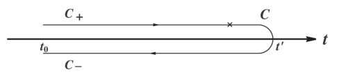
Figure 2.1: The contour $\mathcal{C}$ along the time axis used to evaluate the generating functional for nonequilibrium Green’s functions. It consists of a forward branch $\mathcal{C}_{+}$ running from $t_{0}$ to $t^{\prime}$ and a backward branch $\mathcal{C}_{-}$ from $t^{\prime}$ back to $t_{0}$. The cross denotes insertion of an operator.

For later convenience in the construction of the nonequilibrium Green’s functions, we will introduce sources $J^{\pm}$ coupled to the field operator $\Phi$ in the time evolution operators. The nonequilibrium generating functional is defined as

$$Z[J^{+},J^{-}]\equiv\mathrm{Tr}[\rho\,U(t_{0},t^{\prime};J^{-})\,U(t^{\prime},t_{0};J^{+})],$$ (2.5)

where $U(t,t^{\prime};J)$ denotes the time evolution operator in the presence of the external source $J$. Note that in general $J^{+}\neq J^{-}$, so that $Z[J^{+},J^{-}]$ depends on two different sources. If these are set equal, one has $Z[J,J]=\mathrm{Tr}\,\rho$, which is equal to unity after proper normalization, being a statement of unitarity.

The functional $Z[J^{+},J^{-}]$ can be represented as a path integral by imposing boundary conditions in terms of complete sets of eigenstates of the Schrödinger field operator $\Phi$. Making use of the completeness of eigenstates and the path integral representation for the time evolution operators, one obtains the following path integral representation for $Z[J^{+},J^{-}]$:

$$Z[J^{+},J^{-}] = \int D\phi_{1}\,D\phi_{2}\,\langle\phi_{1}|\rho|\phi_{2}\rangle\int D\varphi\int_{\phi_{1}}^{\varphi}\mathcal{D}\Phi^{+}\int_{\phi_{2}}^{\varphi}\mathcal{D}\Phi^{-}$$ (2.6)

$$\times\,\exp\left[i\int_{t_{0}}^{t^{\prime}}dt\,d^{3}x\Big{(}\mathcal{L}[\Phi^{+}]-\mathcal{L}[\Phi^{-}]+J^{+}\Phi^{+}-J^{-}\Phi^{-}\Big{)}\right],$$

where $\Phi^{+}$ ($\Phi^{-}$) refers to field defined on the forward $\mathcal{C}_{+}$ (backward $\mathcal{C}_{-}$) branch and $\mathcal{L}[\Phi]$ is the Lagrangian density. We note that in above functional expression $\Phi^{+}$ and $\Phi^{-}$ are not independent variables, but are linked through the boundary conditions at time $t^{\prime}$ in the future. To circumvent this difficulty, we will take $t^{\prime}\rightarrow\infty$ for all practical purpose and treat $\Phi^{+}$ and $\Phi^{-}$ as independent variables.

The generating functional $Z[J^{+},J^{-}]$ can be written in a compact path-ordered form

$$Z[J_{c}] = \int D\phi_{1}\,D\phi_{2}\,\langle\phi_{1}|\rho|\phi_{2}\rangle\int_{\phi_{1}}^{\phi_{2}}\mathcal{D}\Phi_{c}\,\exp\left[i\int_{\mathcal{C}}dt\,d^{3}x\Big{(}\mathcal{L}[\Phi_{c}]+J_{c}\,\Phi_{c}\Big{)}\right],$$ (2.7)

where

$$\Phi_{c}=\left\{\begin{array}[]{l}\Phi^{+}\quad\mathrm{for}\quad t\in\mathcal{C}_{+}\\ \Phi^{-}\quad\mathrm{for}\quad t\in\mathcal{C}_{-}\end{array},\right.\quad\quad J_{c}=\left\{\begin{array}[]{l}J^{+}\quad\mathrm{for}\quad t\in\mathcal{C}_{+}\\ J^{-}\quad\mathrm{for}\quad t\in\mathcal{C}_{-}\end{array},\right.$$ (2.8)

and

$$\int_{\mathcal{C}}dt=\int^{\infty}_{t_{0}\;\mathcal{C}_{+}}dt-\int^{\infty}_{t_{0}\;\mathcal{C}_{-}}dt$$ (2.9)

accounting for the opposite direction of integration along the backward time branch.

The above results are very general and are valid for any initial density matrix $\rho$. In fact, as can be seen from Eqs. (2.6) and (2.7), the only effect of the initial density matrix $\rho$ is to specify the boundary conditions for the path integral at $t_{0}$ through the matrix element $\langle\phi_{1}|\rho|\phi_{2}\rangle$, thus in turn to impose the boundary conditions on the nonequilibrium Green’s functions. This means that the equations of motion for the Green’s functions at $t>t_{0}$ are not influenced by the presence of the initial density matrix.

We note that it is always possible to express the matrix element of the initial density matrix as an exponential of a polynomial in the fields [39, 40]:

$$\langle\phi_{1}|\rho|\phi_{2}\rangle=e^{-K[\phi_{1},\phi_{2}]},$$ (2.10)

where

$$K[\phi_{1},\phi_{2}]=K+\int d^{3}x\,K_{a}(\mathbf{x})\phi_{a}(\mathbf{x})+\int d^{3}x\,d^{3}y\,\phi_{a}(\mathbf{x})K_{ab}(\mathbf{x},\mathbf{y})\phi_{b}(\mathbf{y})+\cdots,$$ (2.11)

with $a,b=1,2$. In the above expression the constant $K$ can be absorbed into the normalization and the various coefficient functions $K_{a}(\mathbf{x})$, $K_{ab}(\mathbf{x},\mathbf{y})$, etc., have the interpretations of initial conditions on the one-point (mean field), two-point correlation functions, etc., which contain all the information of the initial density matrix $\rho$. For an initial density matrix which is diagonal in the basis of the (quasi)particle number operators, it can be shown that all the initial correlation functions higher than two point vanish.

Perturbation theory and Feynman rules

The most convenient feature of the CTP formalism of nonequilibrium quantum field theory is that it is formally analogous to standard quantum field theory, except for the fact that the fields have contributions from both time branches. In particular, as in usual field theory, one obtains from variations of the generating functional $Z[J^{+},J^{-}]$ (or, equivalently, $Z[J_{c}]$) the nonequilibrium Green functions, which, however, now include all correlations between points on either forward and backward time branches. The path-ordered $n$-particle ($2n$-point) Green’s function is defined by

$$G_{c}(x_{1}\ldots x_{n},x^{\prime}_{1}\ldots x^{\prime}_{n})=i^{\,n}\,\langle\mathcal{T}_{c}\Phi(x_{1})\ldots\Phi(x_{n})\Phi(x^{\prime}_{n})\ldots\Phi(x^{\prime}_{1})\rangle,$$ (2.12)

with

$$\langle\mathcal{T}_{c}\Phi(x_{1})\ldots\Phi(x_{n})\Phi(x^{\prime}_{n})\ldots\Phi(x^{\prime}_{1})\rangle=(-i)^{2n}\prod_{i=1}^{n}\left.\frac{\delta}{\delta J_{c}(x_{i})}\frac{\delta}{\delta J_{c}(x^{\prime}_{i})}\ln Z[J_{c}]\right|_{J_{c}=0},$$

where $\mathcal{T}_{c}$ is the contour ordering operator along the closed contour $\mathcal{C}$. Although for physical observables the time arguments are on the forward branch, both forward and backward branches will come into play at intermediate steps in a self-consistent calculation.

For instance, there are four types of single-particle (two-point) Green’s functions (i.e., propagators) to be given by (here we have suppressed the space arguments for notational simplicity)

$$G^{++}(t,t^{\prime}) = \pm\,i\,\langle\mathcal{T}\Phi(t)\bar{\Phi}(t^{\prime})\rangle$$

$$= G^{>}(t,t^{\prime})\theta(t-t^{\prime})+G^{<}(t,t^{\prime})\theta(t^{\prime}-t),$$

$$G^{--}(t,t^{\prime}) = \pm\,i\,\langle\overline{\mathcal{T}}\Phi(t)\bar{\Phi}(t^{\prime})\rangle$$

$$= G^{>}(t,t^{\prime})\theta(t^{\prime}-t)+G^{<}(t,t^{\prime})\theta(t-t^{\prime}),$$

$$G^{-+}(t,t^{\prime}) = \pm\,i\,\langle\Phi(t)\bar{\Phi}(t^{\prime})\rangle\;=\;G^{>}(t,t^{\prime}),$$

$$G^{+-}(t,t^{\prime}) = i\,\langle\bar{\Phi}(t^{\prime})\Phi(t)\rangle\;=\;G^{<}(t,t^{\prime}),$$ (2.13)

where $\mathcal{T}$ ($\overline{\mathcal{T}}$) is the (anti)time-ordering operator, the upper (lower) sign refers to Bose (Fermi) fields, $\theta(t-t^{\prime})$ is the Heaviside step function and $\bar{\Phi}\equiv\Phi^{\dagger}$ for bosons but $\bar{\Psi}\equiv\Psi^{\dagger}\gamma^{0}$ for Dirac fermions. These nonequilibrium Green’s functions are not completely independent of each other, instead they are related by the relation

$$G^{++}(t,t^{\prime})+G^{--}(t,t^{\prime})-G^{-+}(t,t^{\prime})-G^{+-}(t,t^{\prime})=0,$$ (2.14)

where use has been made of the identity $\theta(t-t^{\prime})+\theta(t^{\prime}-t)=1$. Furthermore, we can define the retarded and advanced Green’s functions, respectively, by

$$G_{R}(t,t^{\prime}) = G^{++}(t,t^{\prime})-G^{+-}(t,t^{\prime})$$

$$= [G^{>}(t,t^{\prime})-G^{<}(t,t^{\prime})]\,\theta(t-t^{\prime}),$$

$$G_{A}(t,t^{\prime}) = G^{++}(t,t^{\prime})-G^{-+}(t,t^{\prime})$$ (2.15)

$$= [G^{<}(t,t^{\prime})-G^{>}(t,t^{\prime})]\,\theta(t^{\prime}-t).$$

We note that the Wightman functions $G^{\gtrless}(t,t^{\prime})$ determine uniquely the nonequilibrium single-particle Green’s functions, thus playing important roles in nonequilibrium quantum field theory. In equilibrium $G(x,x^{\prime})=G(x-x^{\prime})$ and the space-time Fourier transform of the Green’s functions have specific analytic properties that allow to extract dispersion relations that are important to our later discussion.

One can then construct a diagrammatic perturbative expansion of the Green’s functions much in the same manner as in usual field theory by decomposing the full Lagrangian into the free field (noninteracting) part $\mathcal{L}_{0}$ and the interaction part $\mathcal{L}_{\mathrm{int}}$ and treating the latter as perturbation. The doubling of the sources, fields and integration contours in the nonequilibrium generating functional results in an effective nonequilibrium CTP Lagrangian density [see Eq. (2.6)]

$$\mathcal{{L}}_{\mathrm{CTP}}[\Phi^{+},\Phi^{-}]=\mathcal{{L}}[\Phi^{+}]-\mathcal{L}[\Phi^{-}]~{},$$ (2.16)

which in turn leads to the following nonequilibrium Feynman rules in perturbation theory:

1. There are two types of interaction vertices, corresponding to fields defined on the forward and backward time branch. The vertices associated with fields on the forward branch are the usual interaction vertices, while those associated with fields on the backward branch have the opposite sign.

2. There are four kinds of free field single-particle Green’s functions (propagators), corresponding to the possible contractions of fields among the two branches [see Eq. (2.13)]. Besides the usual time-ordered propagators which are associated with correlations of fields on the forward branch, there are antitime-ordered propagators associated with correlation of fields on the backward branch as well as the unordered Wightman functions associated with correlation of fields on different branches.

3. The combinatoric factors, rules for loop (time and momentum) integrals, etc., remain the same as in usual field theory.

In this thesis we study two different types of nonequilibrium phenomena in quantum field theoretical systems: the relaxation of mean fields in the linearized approximation (i.e., linear response theory) and the quantum kinetic equation that describes the time evolution of the single-(quasi)particle distribution function, hence we will specify below in Sec. 2.2 the initial density matrix $\rho$ used in each case.

2.2 Initial Value Problems in Quantum Field Theory

The initial value formulation provides a convenient description for studying the time evolution of dynamical systems, ranging from Hamilton’s equations, kinetic equations and hydrodynamical equations in classical physics to the time-dependent Schrödinger equation in nonrelativistic quantum mechanics. The fundamental ingredients of initial value problems are the equations of motion, which govern the dynamical evolution, and the initial conditions, which contain all the dynamics prior to some initial time $t_{0}$ from which on the evolution of the state is followed. The advantage of the initial value formulation is that the dynamics of the system for times $t>t_{0}$ will be determined once the equations of motions and initial condition are prescribed.

When one studies relativistic quantum field theory, however, one generally does not use the initial value formulation, instead a quite different approach to relativistic quantum field theory based on $S$-matrix elements was developed. The main reason for this is that the majority of problems to which the theory has been applied do not require knowledge of the detailed time evolution of the system. Indeed, as mentioned in the beginning of this chapter, the typical quantity of experimental interest is the cross section, which is most easily calculated in terms of the $S$-matrix elements. Thus, an initial value formulation in relativistic quantum field seems superfluous.

Nevertheless, as emphasized in the Introduction, recent development in cosmology, ultrarelativistic heavy ion collisions and condensed matter physics reveals that there are a wide variety of physically interesting questions which require not only a quantum field-theoretical description but also a thorough understanding of the time evolution of these systems. Clearly, one must depart from the usual description in terms of the time-independent $S$-matrix element and treat the dynamics with the full time evolution.

The rest of this chapter is devoted to an introduction to two important initial value problems for studying nonequilibrium dynamics in quantum field theory: linear relaxation of the mean fields and quantum kinetic theory.

2.2.1 Linear relaxation of mean fields

The mean fields under consideration are the expectation value of field operators in the nonequilibrium state induced by the external time-dependent perturbations. Our strategy to study the irreversible relaxation (damping) of these mean fields as initial value problems is to prepare these mean fields for a system via adiabatic switching-on of an external perturbation from the remote past. Once the external perturbations are switched off at time $t=0$, the induced mean fields must relax towards equilibrium and we aim to study this nonequilibrium dynamics in linear response theory [41, 42, 43] directly in real time.

To illustrate all the relevant physics and avoid the complexity associated with the issue of thermalization, we assume the system at $t_{0}=-\infty$ is described by the free (quasi)particle Hamiltonian $H_{0}$ and in thermodynamical equilibrium at a temperature $T$. We further assume that the interaction Hamiltonian $H_{\mathrm{int}}$ is adiabatically turned on while we prepare the mean fields via adiabatic switching-on the external perturbation. This allows the induced mean fields to be “dressed” adiabatically by the interaction and external perturbation during the preparation time. Hence in this case the initial density matrix $\rho$ at time $t_{0}=-\infty$ has the form $\rho=\exp(-\beta H_{0})/\mathrm{Tr}[\exp(-\beta H_{0})]$, where $\beta=1/T$ is the inverse temperature.

The initial value formulation for studying the linear relaxation (damping) of the mean fields begins by introducing c-number external sources $J(x)$ coupled to generic (Bose or Fermi) quantum fields $\Phi(x)$. In the presence of external perturbation the effective CTP Lagrangian density becomes

$$\mathcal{L}_{\mathrm{CTP}}[\Phi^{+}(x),\Phi^{-}(x)]=\mathcal{L}[\Phi^{+}(x)]+\left[J(x)\,\Phi^{+}(x)+\mathrm{H.c.}\right]-(\Phi^{+}\to\Phi^{-}).$$ (2.17)

The presence of external sources will induce responses of the system. The expectation value of $\Phi(x)$ induced by $J(x)$ in a linear response analysis is given by

$$\phi({\bf x},t) \equiv \langle\Phi^{\pm}({\bf x},t)\rangle_{J}$$ (2.18)

$$= \pm\int_{t_{0}}^{\infty}dt^{\prime}\int d^{3}x^{\prime}\,G_{R}({\mathbf{x}},t;{\mathbf{x}^{\prime}},t^{\prime})\,J({\mathbf{x}^{\prime}},t^{\prime}),$$

where the upper (lower) sign in the second equality refers to Bose (Fermi) fields and $G_{R}(\mathbf{x},t;\mathbf{x}^{\prime},t^{\prime})$ is the retarded Green’s function defined in Eq. (2.15):

$$G_{R}(\mathbf{x},t;\mathbf{x}^{\prime},t^{\prime}) = \pm\,i\left[\left\langle\Phi^{\pm}(\mathbf{x},t)\bar{\Phi}^{+}(\mathbf{x}^{\prime},t^{\prime})\right\rangle-\left\langle\Phi^{\pm}(\mathbf{x},t)\bar{\Phi}^{-}(\mathbf{x}^{\prime},t^{\prime})\right\rangle\right]$$ (2.19)

$$= \pm\,i\left\langle\left[\Phi(\mathbf{x},t),\bar{\Phi}(\mathbf{x^{\prime}},t^{\prime})\right]_{\mp}\right\rangle\,\theta(t-t^{\prime})$$

$$= [G^{>}(\mathbf{x},t;\mathbf{x}^{\prime},t^{\prime})-G^{<}(\mathbf{x},t;\mathbf{x}^{\prime},t^{\prime})]\,\theta(t-t^{\prime}).$$

In the above, $[\,\cdot\,,\,\cdot\,]_{\mp}$ denotes commutator ($-$) for bosons and anticommutator ($+$) for fermions and, as before, $\bar{\Phi}\equiv\Phi^{\dagger}$ for bosons but $\bar{\Psi}\equiv\Psi^{\dagger}\gamma^{0}$ for Dirac fermions. We emphasize that in Eq. (2.19) the expectation values are calculated in the CTP formalism with full Lagrangian density $\mathcal{L}$, but in the absence of external source as befits the linear response approach.

As explained above, a practically useful initial value formulation for the real-time relaxation of the mean field is obtained by considering that the external source is adiabatically switched on in time from $t_{0}=-\infty$ and suddenly switched off at $t=0$, i.e.,

$$J({\mathbf{x}},t)=J({\mathbf{x}})\,e^{\varepsilon t}\,\theta(-t),\quad\varepsilon\rightarrow 0^{+}.$$ (2.20)

For $t>0$, after the external perturbation has been switched off, the mean field will relax towards its equilibrium value and our aim is to study this relaxation directly in real time.

For the study of linear relaxation of the mean fields, we assume that the system is in thermal equilibrium at a temperature $T$ at time $t=-\infty$ with $\phi(\mathbf{x},t=-\infty)=0$. The retarded and equilibrium (i.e., translational invariant in time) nature of $G_{R}(\mathbf{x},t;\mathbf{x^{\prime}},t^{\prime})$ and the adiabatic switching on of $J({\mathbf{x}},t)$ entail that

$$\phi(\mathbf{x},t=0)=\phi_{0}(\mathbf{x}),\quad\dot{\phi}(\mathbf{x},t<0)=0,$$ (2.21)

where $\phi_{0}(\mathbf{x})$ is determined by $J(\mathbf{x})$ [and vice versa, $\psi_{0}(\mathbf{x})$ can be used to fix $J(\mathbf{x})$] and, here and henceforth, an overdot denotes time derivative. We note that $\dot{\phi}(\mathbf{x},t=0)$ is unspecified even though $\dot{\phi}(\mathbf{x},t<0)=0$. This is because the external source is instantaneous switched off at $t=0$. In fact there could be initial time singularities associated with our choice of the external source given in Eq. (2.20). It has been shown in Ref. [44] that the long-time behavior is insensitive to the initial time singularities, hence we will not address this issue here as it is beyond the scope of this thesis.

In order to study the relaxation of the mean field $\phi(\mathbf{x},t)$ for $T>0$, we need to relate the linear response problem to an initial value problem for the equation of motion of the mean field. This can be achieved by considering the following formal equation of motion for the mean field

$$D\circ\phi(\mathbf{x},t)=\pm\,J(\mathbf{x},t),$$ (2.22)

where the upper (lower) sign refers to Bose (Fermi) fields and the (integro-differential) operator $D$ is the inverse of the retarded Green’s function $G_{R}$. The source $J(x)$ is given by Eq. (2.20) and $\phi(x)$ satisfies the condition Eq. (2.21) at $t=0$. For $t<0$, on the one hand, Eq. (2.22) is exactly the linear response problem Eq. (2.18) satisfying the condition Eq. (2.21) at $t=0$; for $t>0$, on the other hand, it describes the time evolution of the mean field $\phi(\mathbf{x},t)$ with the initial condition specified by Eq. (2.21).

It is at this stage where the nonequilibrium CTP formalism provides the most powerful framework. The real-time equation of motion for the mean field $\phi(x)$ can be obtained via the tadpole method [45], which automatically leads to a retarded and causal initial value problem for the mean field $\phi(x)$.

The central idea of the tadpole method is to write the field into the $c$-number expectation value plus quantum fluctuations around it, i.e., writing

$$\Phi^{\pm}({\mathbf{x}},t)=\phi({\mathbf{x}},t)+\chi^{\pm}({\mathbf{x}},t),\quad\mbox{with}\quad\langle\chi^{\pm}({\mathbf{x}},t)\rangle=0.$$ (2.23)

The equation of motion for the mean field $\phi({\mathbf{x}},t)$ can be obtained to any order in perturbation theory by requiring the tadpole condition $\langle\chi^{\pm}({\mathbf{x}},t)\rangle=0$ to all orders in perturbation theory [45].

2.2.2 Quantum kinetic theory

The foundation of modern kinetic theory dates back to 1872 when Boltzmann published his famous kinetic equation for dilute gases [46]. The Boltzmann equation is a nonlinear integro-differential equation for the single-particle distribution function, a microscopic quantity introduced by Boltzmann that describes the density of gas molecules in phase space. The success of Boltzmann’s kinetic description for dilute gasses not only provides the first theoretical understanding of macroscopic physics in terms of the underlying microscopic dynamics, but also makes kinetic theory one of the most powerful approaches to transport phenomena in macroscopic systems.

A necessary criterion for the validity of Boltzmann’s kinetic description is that there must be a wide separation of time scales in the system. A classic example is furnished by the derivation of the classical Boltzmann equation: Boltzmann introduced, with great intuition, “molecular chaos” (assumption that particles in a dilute gas are not correlated), which crucially depends upon the fact the duration of each individual collision process is much shorter than the average time that elapse between two successive collisions. Based on Boltzmann’s classical picture of completed collisions, one can easily write down the semiclassical Boltzmann equation, also known as the Uehling-Uhlenbeck equation [47], by modifying the collision term using Fermi’s golden rule (which gives the quantum mechanical transition probability per unit time) and taking into account the quantum statistics of the particles (bosons or fermions). Whereas the semiclassical Boltzmann equation is appealing in describing a variety of transport problems, Boltzmann kinetics is an approximation only and needs to be justified from first principles, especially for quantum systems under extreme nonequilibrium conditions which have been a subject of great theoretical and experimental interest over the last decade.

Although a wide separation of time scales is a necessary condition for the validity of the (semi)classical Boltzmann kinetics, it is far from sufficient. In particular when there is competition of relevant time scales or quantum transient kinetics at early stages is physically important, a full quantum kinetic equation, of which usual Boltzmann kinetics is a semiclassical limit, must be obtained. The most widely used method in the derivation of the quantum kinetic equation is that of nonequilibrium Green’s functions originally developed by Kadanoff and Baym [35]. This method involves Wigner transforms of two-point Green’s functions and eventually a gradient expansion [48, 49]. Such gradient expansion assumes that the center-of-mass Wigner variables are “slowly varying”, but it is seldom clear at this level which are the fast and which are the slow scales involved. A “coarse-graining” procedure is typically invoked that averages out microscopic scales in the kinetic description, leading to irreversible evolution in the resulting kinetic equation. Such an averaging procedure is usually poorly understood and justified a posteriori.

In this thesis, we propose to study quantum kinetics by focusing on a systematic, first-principle derivation of quantum kinetic equations from the underlying quantum field theory. Specifically, we aim to provide a kinetic description of an initially prepared nonequilibrium quantum system by studying the time evolution of the single-particle distribution functions for the relevant degrees of freedom directly in real time.

This novel approach begins by defining a suitable (quasi)particle number operator whose expectation value $n_{\mathbf{k}}(t)$ is interpreted as the single particle distribution function for the relevant degrees of freedom of momentum $\mathbf{k}$ in the presence of the medium, and by separating the total Hamiltonian into the free part that commutates with the (quasi)particle number operator and a interaction part that describes interaction between these (quasi)particles. As a consequence of the medium effects, the above defined (quasi)particles are in general different from the corresponding free particles in the vacuum. In the Heisenberg picture, the time evolution of the distribution function $dn_{\mathbf{k}}(t)/dt$ is obtained by using the Heisenberg equation of motion. Choosing the initial density matrix $\rho$ at a finite initial time $t=t_{0}$ to be diagonal in the basis of the (quasi)particles number operators but with nonequilibrium distributions $n_{\mathbf{k}}(t_{0})$, one can write down a perturbative expansion for $d\,n_{\mathbf{k}}(t)/dt$ as an initial value problem in terms of the initial distribution function. The solution of this initial value problem contains secular terms that grow with time and invalidate the perturbative expansion at large times as a consequence of the fact that perturbation theory neglects the change in the distribution function as time goes on.

We introduce a novel dynamical renormalization group that allows a consistent resummation of secular terms in real time and leads to an improvement of the perturbative expansion that is valid on kinetic time scales. This real-time initial value formulation has the advantage that it displays the relevant microscopic and kinetic time scales, leads to a well-defined coarse-graining procedure, allows a systematic improvement on the kinetic description and, if necessary, consistently includes nonexponential relaxation in a physically intuitive manner.

To conclude this chapter, we emphasize that the main theme of this thesis is describing the dynamical development of a nonequilibrium multiparticle system, which evolves from an initially prepared quantum state. Since the nonequilibrium system is characterized by its dynamical evolution in time, a physically intuitive description of nonequilibrium dynamics is that in terms of the initial value formulation. In this thesis we propose to study real-time relaxation of mean fields and quantum kinetics in quantum multiparticle systems as initial value problems. The CTP formalism of nonequilibrium quantum field theory is a powerful theoretical framework designed to describe directly in real time the expectation values of physical observables in the presence of medium, thus providing a general tool for treating initial value problems of nonequilibrium multiparticle dynamics in quantum field theory.

Chapter 3 Fermion Damping in a Fermion-Scalar Plasma

3.1 Introduction

The propagation of quarks and leptons in a medium of high temperature and/or density is of fundamental importance in a wide variety of physically relevant situations. In stellar astrophysics, electrons and neutrinos play a major role in the evolution of dense stars such as white dwarfs, neutron stars and supernovae [50]. The propagation of quarks during the nonequilibrium stages of the electroweak phase transition is conjectured to be an essential ingredient for baryogenesis at the electroweak scale both in non-supersymmetric and supersymmetric extensions of the standard model [21]. Furthermore, medium effects can enhance neutrino oscillations as envisaged in the Mikheyev-Smirnov-Wolfenstein (MSW) effect [51] and dramatically modify the neutrino electromagnetic couplings [52].

In-medium propagation of particles is dramatically different from that in the vacuum. The medium modifies the dispersion relation of the excitations and introduces a width to the propagating excitation [53, 54, 42, 43] that results in damping of the amplitude of the propagating mode. Whereas the propagation of quarks and leptons in a QED or QCD plasma has been studied thoroughly [55, 43], a similar study for a scalar plasma has not been carried out to the same level of detail. Recently some attention has been given to understanding the thermalization time scales of boson and fermion excitations in a plasma of gauge [56] and scalar bosons [57]. It has also been shown that fermion thermalization is an important ingredient in models of baryogenesis mediated by scalars [58]. Most of the studies of fermion thermalization focus on the mechanism of fermion scattering off the gauge quanta in the heat bath (Landau damping). Although the scalar contribution to the fermion self-energy to one-loop order has been obtained a long time ago [54], scant attention has been paid to a more detailed understanding of the contribution from the scalar degrees of freedom to the fermion relaxation and thermalization. As mentioned above, this issue becomes of pressing importance in models of baryogenesis and more so in models in which the scalars carry baryon number [58].

In this chapter we focus on several aspects of propagation of fermion excitations in a fermion-scalar plasma. Specifically, we offer a detailed and general study of fermion relaxation and thermalization through the interactions with the scalars in the plasma directly in real time for arbitrary scalar and fermion masses, temperature and fermion momentum. More importantly, we focus on a novel mechanism of damping for fermion excitations that occurs whenever the effective mass of the scalar particle allows its kinematic decay into fermion pairs. This phenomenon only occurs in the medium and is interpreted as an induced damping due to the presence of scalars in the medium. It is a process different from collisional damping and Landau damping which are the most common processes that lead to relaxation and thermalization. This process results in new thermal cuts in the fermion self-energy and, for heavy scalars, a quasiparticle pole structure in the fermion propagator that provides a finite width to the fermion excitation. The remarkable and perhaps nonintuitive aspect of our analysis is that the decay of the scalar in the medium leads to damping of the fermion excitations and their propagation as quasiparticle resonances.

The effective real-time Dirac equation in the medium allows a direct interpretation of the damping of the fermion excitation and leads to a clear definition of the damping rate. By analyzing the quasiparticle wave functions we obtain an all-order expression for the damping rate that confirms and generalizes recent results for the massless chiral case [59, 60].

In order to provide a complementary understanding of the process of induced decay of the heavy scalars in the medium and the resulting fermion damping, we study relaxation of the fermion distribution function by using a semiclassical Boltzmann equation. Linearizing the Boltzmann equation near the equilibrium distribution, we obtain the relation between the thermalization rate for the distribution function in the relaxation time approximation and the damping rate for the amplitude of the fermion mean fields to lowest order in the Yukawa coupling. This analysis provides a real-time confirmation of the oft quoted relation between the interaction rate (obtained from the Boltzmann kinetic equation in the relaxation time approximation) and the damping rate for the mean field [54, 43]. More importantly, this analysis reveals directly, via a kinetic approach in real time how the process of induced decay of a heavy scalar in the medium results in damping and thermalization of the fermion excitations. A study of the relation between the interaction rate and the damping rate has been presented recently for gauge theories within the context of the imaginary time formulation [61]. Our results provide a real-time confirmation for the scalar case.

This chapter is organized as follows. In Sec. 3.2 we obtain the renormalized effective in-medium Dirac equation for the fermion mean field in real time starting from the linear response to an external (Grassmann) source that induces the mean field. The renormalization aspects are addressed in detail. We then study in detail the structure of the renormalized fermion self-energy and establish the presence of new cuts of thermal origin. In Sec. 3.3 we present a real-time analysis of the evolution of the fermion mean field and clarify the difference between complex poles and resonances (often misunderstood). An analysis of the structure of the self-energy and an interpretation of the exact quasiparticle spinor wave functions allows us to provide an all-order expression for the damping rate of the fermion mean fields. In Sec. 3.4 we present an analysis of the evolution of the fermion distribution function in real time by obtaining a (Boltzmann) kinetic equation in the relaxation time approximation. We clarify to lowest order the relation between the damping rate of the fermion excitations and the interaction rate of the distribution function. In Sec. 3.5 we summarize our results.

3.2 Effective Dirac Equation in the Medium

As mentioned in the Introduction, whereas the damping of collective and quasiparticle excitations via the interactions with gauge bosons in the medium has been the focus of most attention, understanding of the influence of scalars has not been pursued so vigorously.

Although we are ultimately interested in studying the damping of fermion excitations in a plasma with scalars and gauge fields within the realm of electroweak baryogenesis in either the Standard Model or generalizations thereof, we will begin by considering only the coupling of a massive Dirac fermion to a scalar via a simple Yukawa interaction. The model dependent generalizations of the Yukawa couplings to particular cases will differ quantitatively in the details of the group structure but the qualitative features of the effective Dirac equation in the medium as well as the kinematics of the thermal cuts that lead to damping of the fermion excitations will be rather general.

We consider a Dirac fermion $\Psi$ with the bare mass $M_{0}$ coupled to a scalar $\phi$ with the bare mass $m_{0}$ via a bare Yukawa coupling $y_{0}$. The bare fermion mass could be the result of spontaneous symmetry breaking in the scalar sector, but for the purposes of our studies we need not specify its origin. The Lagrangian density is given by

$$\mathcal{L}[\Psi,\phi]=\bar{\Psi}(i{\not\!{\partial}}-M_{0})\Psi+\frac{1}{2}\partial_{\mu}\phi\,\partial^{\mu}\phi-\frac{1}{2}m_{0}^{2}\phi^{2}-{\cal L}_{I}[\phi]-y_{0}\bar{\Psi}\phi\Psi+\bar{\eta}\Psi+\bar{\Psi}\eta+j\phi.$$ (3.1)

The self-interaction of the scalar field accounted for by the term ${\cal L}_{I}[\phi]$ need not be specified to lowest order. In the above expression, $\eta$ and $j$ are the respective external fermionic and scalar sources that are introduced in order to provide an initial value problem for fermion relaxation. We now write the bare fields and sources in terms of the renormalized quantities (referred to with a subscript $r$) by introducing the renormalization constants and counterterms:

$$\Psi=Z_{\psi}^{1/2}\,\Psi_{r},\quad\phi=Z_{\phi}^{1/2}\,\phi_{r},\quad\eta=Z_{\psi}^{-1/2}\eta_{r},\quad j=Z_{\phi}^{-1/2}j_{r},$$

$$y=y_{0}Z_{\phi}^{1/2}Z_{\psi}/Z_{y},\quad m^{2}_{0}=\left(\delta_{m}+m^{2}\right)/Z_{\phi},\quad M_{0}=\left(\delta_{M}+M\right)/Z_{\psi}.$$ (3.2)

With the above definitions, the Lagrangian can be rewritten as (here and henceforth, we have suppressed the subscript $r$ for notational simplicity)

$${\cal{L}} = \bar{\Psi}(i{\not\!{\partial}}-M)\Psi+\frac{1}{2}\partial_{\mu}\phi\,\partial^{\mu}\phi-\frac{1}{2}m^{2}\phi^{2}-\mathcal{L}_{I}[\phi]-y\bar{\Psi}\phi\Psi+\bar{\eta}\Psi+\bar{\Psi}\eta+j\phi$$ (3.3)

$$+\,\frac{1}{2}\delta_{\phi}\partial_{\mu}\phi\,\partial^{\mu}\phi-\frac{1}{2}\delta_{m}\phi^{2}+\bar{\Psi}(i\delta_{\psi}{\not\!{\partial}}-\delta_{M})\Psi-y\delta_{y}\bar{\Psi}\phi\Psi+\delta\mathcal{L}^{c}_{I}[\phi],$$

where $m$ and $M$ are the renormalized masses, and $y$ is the renormalized Yukawa coupling. The terms with the coefficients

$$\delta_{\psi}=Z_{\psi}-1,\quad\delta_{\phi}=Z_{\phi}-1,\quad\delta_{M}=Z_{\psi}M_{0}-M,\quad\delta_{m}=Z_{\phi}\,m^{2}_{0}-m^{2},\quad\delta_{y}=Z_{y}-1,$$

and $\delta\mathcal{L}^{c}_{I}$ are the counterterms to be determined consistently in the perturbative expansion by choosing a renormalization prescription. As it will become clear below this is the most natural manner for obtaining a fully renormalized Dirac equation in a perturbative expansion.

Our goal is to understand the relaxation of inhomogeneous fermion mean field $\psi(\mathbf{x},t)=\langle\Psi(\mathbf{x},t)\rangle$ induced by external source that is adiabatically switched-on at $t=-\infty$. As explained in Sec. 2.2, the equation of motion for the mean field can be obtained to any order in perturbative theory via the tadpole method [45] by writing

$$\Psi^{\pm}(\mathbf{x},t)=\psi(\mathbf{x},t)+\chi^{\pm}(\mathbf{x},t),\quad\mbox{with}\quad\langle\chi^{\pm}(\mathbf{x},t)\rangle=0.$$ (3.4)

The essential ingredients for perturbative calculations are the following free real-time Green’s functions (in momentum space):

(i) Scalar Propagators

$$G_{0}^{++}(\mathbf{k},t,t^{\prime}) = G_{0}^{>}(\mathbf{k},t,t^{\prime})\,\theta(t-t^{\prime})+G_{0}^{<}(\mathbf{k},t,t^{\prime})\,\theta(t^{\prime}-t),$$

$$G_{0}^{--}(\mathbf{k},t,t^{\prime}) = G_{0}^{>}(\mathbf{k},t,t^{\prime})\,\theta(t^{\prime}-t)+G_{0}^{<}(\mathbf{k},t,t^{\prime})\,\theta(t-t^{\prime}),$$

$$G_{0}^{-+}(\mathbf{k},t,t^{\prime}) = G_{0}^{>}(\mathbf{k},t,t^{\prime}),\quad G_{0}^{+-}(\mathbf{k},t,t^{\prime})=G_{0}^{<}(\mathbf{k},t,t^{\prime}),$$

$$G_{0}^{>}(\mathbf{k},t,t^{\prime}) = i\int d^{3}x\,e^{-i\mathbf{k}\cdot\mathbf{x}}\,\langle\phi(\mathbf{x},t)\phi(\mathbf{0},t^{\prime})\rangle$$

$$= \frac{i}{2\omega_{\mathbf{k}}}\left[[1+n_{B}(\omega_{\mathbf{k}})]\,e^{-i\omega_{\mathbf{k}}(t-t^{\prime})}+n_{B}(\omega_{\mathbf{k}})\,e^{i\omega_{\mathbf{k}}(t-t^{\prime})}\right],$$

$$G_{0}^{<}(\mathbf{k},t,t^{\prime}) = i\int d^{3}x\,e^{-i\mathbf{k}\cdot\mathbf{x}}\,\langle\phi(\mathbf{0},t^{\prime})\phi(\mathbf{x},t)\rangle$$ (3.5)

$$= \frac{i}{2\omega_{\mathbf{k}}}\left[n_{B}(\omega_{\mathbf{k}})\,e^{-i\omega_{\mathbf{k}}(t-t^{\prime})}+[1+n_{B}(\omega_{\mathbf{k}})]\,e^{i\omega_{\mathbf{k}}(t-t^{\prime})}\right],$$

where $\omega_{\mathbf{k}}=\sqrt{\mathbf{k}^{2}+m^{2}}$ and $n_{B}(\omega)=1/(e^{\beta\omega}-1)$ is the Bose-Einstein distribution.

(ii) Fermion Propagators (zero fermion chemical potential)

$$S_{0}^{++}(\mathbf{k},t,t^{\prime}) = S_{0}^{>}(\mathbf{k},t,t^{\prime})\,\theta(t-t^{\prime})+S_{0}^{<}(\mathbf{k},t,t^{\prime})\,\theta(t^{\prime}-t),$$

$$S_{0}^{--}(\mathbf{k},t,t^{\prime}) = S_{0}^{>}(\mathbf{k},t,t^{\prime})\,\theta(t^{\prime}-t)+S_{0}^{<}(\mathbf{k},t,t^{\prime})\,\theta(t-t^{\prime}),$$

$$S_{0}^{-+}(\mathbf{k},t,t^{\prime}) = S_{0}^{>}(\mathbf{k},t,t^{\prime}),\quad S_{0}^{+-}(\mathbf{k},t,t^{\prime})=S_{0}^{<}(\mathbf{k},t,t^{\prime}),$$

$$S_{0}^{>}(\mathbf{k},t,t^{\prime}) = -i\int d^{3}x\,e^{-i\mathbf{k}\cdot\mathbf{x}}\,\langle\Psi(\mathbf{x},t)\bar{\Psi}(\mathbf{0},t^{\prime})\rangle$$

$$= -\frac{i}{2\bar{\omega}_{\mathbf{k}}}\Big{[}(\gamma^{0}\bar{\omega}_{\mathbf{k}}-\boldsymbol{\gamma}\cdot\mathbf{k}+M)[1-n_{F}(\bar{\omega}_{\mathbf{k}})]\,e^{-i\bar{\omega}_{\mathbf{k}}(t-t^{\prime})}$$

$$+\,(\gamma^{0}\bar{\omega}_{\mathbf{k}}+\boldsymbol{\gamma}\cdot\mathbf{k}-M)\,n_{F}(\bar{\omega}_{\mathbf{k}})\,e^{i\bar{\omega}_{\mathbf{k}}(t-t^{\prime})}\Big{]},$$

$$S_{0}^{<}(\mathbf{k},t,t^{\prime}) = i\int d^{3}x\,e^{-i\mathbf{k}\cdot\mathbf{x}}\,\langle\bar{\Psi}(\mathbf{0},t^{\prime})\Psi(\mathbf{x},t)\rangle$$ (3.6)

$$= \frac{i}{2\bar{\omega}_{\mathbf{k}}}\Big{[}(\gamma^{0}\bar{\omega}_{\mathbf{k}}+\boldsymbol{\gamma}\cdot\mathbf{k}-M)\,n_{F}(\bar{\omega}_{\mathbf{k}})\,e^{-i\bar{\omega}_{\mathbf{k}}(t-t^{\prime})}$$

$$+\,(\gamma^{0}\bar{\omega}_{\mathbf{k}}+\boldsymbol{\gamma}\cdot\mathbf{k}-M)\,[1-n_{F}(\bar{\omega}_{\mathbf{k}})]\,e^{i\bar{\omega}_{\mathbf{k}}(t-t^{\prime})}\Big{]},$$

where $\bar{\omega}_{\mathbf{k}}=\sqrt{\mathbf{k}^{2}+M^{2}}$ and $n_{F}(\omega)=1/(e^{\beta\omega}+1)$ is the Fermi-Dirac distribution. We note that these free propagators given in Eqs. (3.5) and (3.6) are thermal because, as discussed in Sec. 2.2, the initial state is chosen to be in thermal equilibrium and the interaction is assumed to be turned on adiabatically.

In momentum space, we find the effective real-time Dirac equation for the mean field of momentum $\mathbf{k}$ reads

$$\left[\left(i\gamma^{0}\partial_{t}-\boldsymbol{\gamma}\cdot\mathbf{k}-M\right)+\delta_{\psi}\left(i\gamma^{0}\partial_{t}-\boldsymbol{\gamma}\cdot\mathbf{k}\right)-\delta_{M}\right]\psi(\mathbf{k},t)\hskip 72.26999pt$$

$$\hskip 144.54pt-\int_{-\infty}^{t}dt^{\prime}\,\Sigma(\mathbf{k},t-t^{\prime})\,\psi(\mathbf{k},t^{\prime})=-\eta(\mathbf{k},t),$$ (3.7)

where $\partial_{t}\equiv\partial/\partial t$, $\Sigma(\mathbf{k},t-t^{\prime})$ is the retarded fermion self-energy and

$$\psi(\mathbf{k},t)\equiv\int d^{3}x\,e^{-i\mathbf{k}\cdot\mathbf{x}}\,\psi(\mathbf{x},t).$$

Using the real-time free scalar and fermion propagators given by Eqs. (3.5) and (3.6), respectively, we find to one-loop order, that $\Sigma(\mathbf{k},t-t^{\prime})$ is given by

$$\Sigma(\mathbf{k},t-t^{\prime})=i\gamma^{0}\,\Sigma^{(0)}(\mathbf{k},t-t^{\prime})+\boldsymbol{\gamma}\cdot\mathbf{k}\,\Sigma^{(1)}(\mathbf{k},t-t^{\prime})+\Sigma^{(2)}(\mathbf{k},t-t^{\prime}),$$ (3.8)

with

$$\Sigma^{(0)}(\mathbf{k},t-t^{\prime}) = -y^{2}\int\frac{d^{3}q}{(2\pi)^{3}}\frac{1}{2\omega_{\mathbf{p}}}\Big{[}\cos[(\omega_{\mathbf{p}}+\bar{\omega}_{\mathbf{q}})(t-t^{\prime})]\,[1+n_{B}(\omega_{\mathbf{p}})-n_{F}(\bar{\omega}_{\mathbf{q}})]$$

$$+\,\cos[(\omega_{\mathbf{p}}-\bar{\omega}_{\mathbf{q}})(t-t^{\prime})]\,[n_{B}(\omega_{\mathbf{p}})+n_{F}(\bar{\omega}_{\mathbf{q}})]\Big{]},$$

$$\Sigma^{(1)}(\mathbf{k},t-t^{\prime}) = -y^{2}\int\frac{d^{3}q}{(2\pi)^{3}}\frac{\mathbf{k}\cdot\mathbf{q}}{2k^{2}\omega_{\mathbf{p}}\bar{\omega}_{\mathbf{q}}}\Big{[}\sin[(\omega_{\mathbf{p}}+\bar{\omega}_{\mathbf{q}})(t-t^{\prime})]\,[1+n_{B}(\omega_{\mathbf{p}})$$

$$-\,n_{F}(\bar{\omega}_{\mathbf{q}})]-\sin[(\omega_{\mathbf{p}}-\bar{\omega}_{\mathbf{q}})(t-t^{\prime})]\,[n_{B}(\omega_{\mathbf{p}})+n_{F}(\bar{\omega}_{\mathbf{q}})]\Big{]},$$

$$\Sigma^{(2)}(\mathbf{k},t-t^{\prime}) = -y^{2}\int\frac{d^{3}q}{(2\pi)^{3}}\frac{M}{2\omega_{\mathbf{p}}\bar{\omega}_{\mathbf{q}}}\Big{[}\sin[(\omega_{\mathbf{p}}+\bar{\omega}_{\mathbf{q}})(t-t^{\prime})]\,[1+n_{B}(\omega_{\mathbf{p}})-n_{F}(\bar{\omega}_{\mathbf{q}})]$$ (3.9)

$$-\,\sin[(\omega_{\mathbf{p}}-\bar{\omega}_{\mathbf{q}})(t-t^{\prime})]\,[n_{B}(\omega_{\mathbf{p}})+n_{F}(\bar{\omega}_{\mathbf{q}})]\Big{]},$$

where $\mathbf{p=q+k}$ and $k=|\mathbf{k}|$.

As mentioned before, the source is taken to be switched on adiabatically from $t=-\infty$ and switched off at $t=0$ to provide the initial conditions [see Eq. (2.21)]

$$\psi(\mathbf{k},t=0)=\psi(\mathbf{k},0),\qquad\dot{\psi}(\mathbf{k},t<0)=0.$$ (3.10)

Introducing an auxiliary quantity $\sigma(\mathbf{k},t-t^{\prime})$ defined as

$$\Sigma(\mathbf{k},t-t^{\prime})=\partial_{t^{\prime}}\sigma(\mathbf{k},t-t^{\prime})$$ (3.11)

and imposing $\eta(\mathbf{k},t>0)=0$, we obtain the equation of motion for $t>0$ to be given by

$$\left[\left(i\gamma^{0}\partial_{t}-\boldsymbol{\gamma}\cdot\mathbf{k}-M\right)+\delta_{\psi}\left(i\gamma^{0}\partial_{t}-\boldsymbol{\gamma}\cdot\mathbf{k}\right)-\sigma(\mathbf{k},0)-\delta_{M}\right]\psi_{\mathbf{k}}(t)$$ (3.12)

$$+\int_{0}^{t}dt^{\prime}\,\sigma_{\mathbf{k}}(t-t^{\prime})\,\dot{\psi}_{\mathbf{k}}(t^{\prime})=0.$$

This equation of motion can be solved by Laplace transform as befits an initial value problem. The Laplace transformed equation of motion is given by

$$\left[i\gamma^{0}s-\boldsymbol{\gamma}\cdot\mathbf{k}-M+\delta_{\psi}\left(i\gamma^{0}s-\boldsymbol{\gamma}\cdot\mathbf{k}\right)-\delta_{M}-\sigma(\mathbf{k},0)+s\,\widetilde{\sigma}(s,\mathbf{k})\right]\widetilde{\psi}(s,\mathbf{k})$$ (3.13)

$$=\left[i\gamma^{0}+i\delta_{\psi}\gamma^{0}+\widetilde{\sigma}(s,\mathbf{k})\right]\psi(\mathbf{k},0),$$

where $\widetilde{\psi}(s,\mathbf{k})$ and $\widetilde{\sigma}(s,\mathbf{k})$ are, respectively, the Laplace transforms of $\psi(\mathbf{k},t)$ and $\sigma(\mathbf{k},t)$

$$\widetilde{\psi}(s,\mathbf{k})\equiv\int_{0}^{\infty}dt\,e^{-st}\,\psi(\mathbf{k},t),\quad\widetilde{\sigma}(s,\mathbf{k})\equiv\int_{0}^{\infty}dt\,e^{-st}\,\sigma(\mathbf{k},t),$$

with $\mathrm{Re}\,s>0$.

3.2.1 Renormalization

Before proceeding further, we address the issue of renormalization by analyzing the ultraviolet divergences of the self-energy. As usual the ultraviolet divergences are those of zero temperature field theory, since the finite temperature distribution functions are exponentially suppressed at large momenta [43]. Therefore the ultraviolet divergences are obtained by setting to zero the distribution functions for the scalar and fermion.

With Eq. (3.11), one can write $\sigma(\mathbf{k},t-t^{\prime})$ as

$$\sigma(\mathbf{k},t-t^{\prime})=i\gamma^{0}\sigma^{(0)}(\mathbf{k},t-t^{\prime})+\boldsymbol{\gamma}\cdot\mathbf{k}\,\sigma^{(1)}(\mathbf{k},t-t^{\prime})+\sigma^{(2)}(\mathbf{k},t-t^{\prime}).$$ (3.14)

A straightforward calculation leads to the following ultraviolet divergences

$$\sigma^{(1)}(\mathbf{k},0)\simeq\frac{y^{2}}{16\pi^{2}}\ln\frac{\Lambda}{K},\quad\sigma^{(2)}(\mathbf{k},0)\simeq-\frac{y^{2}M}{8\pi^{2}}\ln\frac{\Lambda}{K},\quad\widetilde{\sigma}^{(0)}(s,\mathbf{k})\simeq\frac{y^{2}}{16\pi^{2}}\ln\frac{\Lambda}{K},$$ (3.15)

where, $\widetilde{\sigma}^{(i)}(s,\mathbf{k})$ ($i=0,1,2$) are the Laplace transform of $\sigma^{(i)}(\mathbf{k},t)$, $\Lambda$ is an ultraviolet momentum cutoff, $K$ is an arbitrary renormalization scale, and “$\simeq$” denotes only the divergent contribution is included. Therefore, the counterterms $\delta_{\psi}$ and $\delta_{M}$ are chosen to be given by

$$\delta_{\psi}=-\frac{y^{2}}{16\pi^{2}}\ln\frac{\Lambda}{K}+\mbox{finite},\quad\delta_{M}=\frac{y^{2}M}{8\pi^{2}}\ln\frac{\Lambda}{K}+\mbox{finite},$$ (3.16)

and the components of the self-energy are rendered finite

$$\widetilde{\sigma}(s,\mathbf{k})+i\gamma^{0}\delta_{\psi}=\mathrm{finite},\quad\sigma(\mathbf{k},0)+\boldsymbol{\gamma}\cdot\mathbf{k}\,\delta_{\psi}+\delta_{M}=\mathrm{finite},$$ (3.17)

The finite parts of the counterterms in Eq. (3.16) are fixed by prescribing a renormalization scheme. There are two important choices of counterterms: (i) determining the counterterms from an on-shell condition, including finite temperature effects and (ii) determining the counterterms from a zero temperature on-shell condition. Obviously these choices only differ by finite quantities, but the second choice allows us to separate the dressing effects of the medium from those in the vacuum. For example, by choosing to renormalize the self-energy with the zero-temperature counterterms on the mass shell, the poles in the particle propagator will have unit residue at zero temperature. Then, in the medium the residues at the finite temperature poles (or the position of the resonances) are finite, smaller than one and determined solely by the properties of the medium. Thus the formulation of the initial value problem as presented here yields an unambiguous separation of the vacuum and in-medium renormalization effects.

Hence we obtain the renormalized effective Dirac equation in the medium and the corresponding initial value problem for the fermion mean field

$$\left[i\gamma^{0}s-\boldsymbol{\gamma}\cdot\mathbf{k}-M-\widetilde{\Sigma}(s,\mathbf{k})\right]\widetilde{\psi}(s,\mathbf{k})=\left[i\gamma^{0}+\widetilde{\sigma}(s,\mathbf{k})\right]\psi(\mathbf{k},0),$$ (3.18)

where $\widetilde{\Sigma}(s,\mathbf{k})=\sigma(\mathbf{k},0)-s\,\widetilde{\sigma}(s,\mathbf{k})$ is the Laplace transform of the renormalized retarded fermion self-energy [see Eq. (3.17)], which can be written in its most general form

$$\widetilde{\Sigma}(s,\mathbf{k})=i\gamma^{0}s\,\widetilde{\mathcal{E}}^{(0)}(s,\mathbf{k})+\boldsymbol{\gamma}\cdot\mathbf{k}\,\widetilde{\mathcal{E}}^{(1)}(s,\mathbf{k})+M\,\widetilde{\mathcal{E}}^{(2)}(s,\mathbf{k}).$$ (3.19)

The solution to Eq. (3.18) is given by

$$\widetilde{\psi}(s,\mathbf{k})=\frac{1}{s}\left\{1+S(s,\mathbf{k})\Big{[}\boldsymbol{\gamma}\cdot\mathbf{k}+M+\widetilde{\Sigma}(0,\mathbf{k})\Big{]}\right\}\psi(\mathbf{k},0),$$ (3.20)

where $S(s,\mathbf{k})$ is the fermion propagator in terms of the Laplace variable $s$

$$S(s,\mathbf{k}) = \left[i\gamma^{0}s-\boldsymbol{\gamma}\cdot\mathbf{k}-M-\widetilde{\Sigma}(s,\mathbf{k})\right]^{-1}$$ (3.21)

$$= -\,\frac{i\gamma^{0}s[1-\widetilde{\mathcal{E}}^{(0)}(s,\mathbf{k})]-\boldsymbol{\gamma}\cdot\mathbf{k}[1+\widetilde{\mathcal{E}}^{(1)}(s,\mathbf{k})]+M[1+\widetilde{\mathcal{E}}^{(2)}(s,\mathbf{k})]}{s^{2}[1-\widetilde{\mathcal{E}}^{(0)}(s,\mathbf{k})]^{2}+k^{2}[1+\widetilde{\mathcal{E}}^{(1)}(s,\mathbf{k})]^{2}+M^{2}[1+\widetilde{\mathcal{E}}^{(2)}(s,\mathbf{k})]^{2}}.$$

We note that the square of the denominator in Eq. (3.21) is recognized as [43]

$$\det\left[i\gamma^{0}s-\boldsymbol{\gamma}\cdot\mathbf{k}-M-\widetilde{\Sigma}(s,\mathbf{k})\right].$$ (3.22)

The real-time evolution of $\psi(\mathbf{k},t)$ is obtained by performing the inverse Laplace transform along the Bromwich contour in the complex $s$-plane parallel to the imaginary axis and to the right of all singularities of $\widetilde{\psi}(s,\mathbf{k})$. Therefore to obtain the real time evolution we must first understand the singularities of the Laplace transform in the complex $s$-plane.

3.2.2 Structure of the self-energy and damping processes

To one-loop order, the Laplace transform of the components $\widetilde{\mathcal{E}}^{(i)}(s,\mathbf{k})$ ($i=0,1,2$) of the fermion self-energy $\widetilde{\Sigma}(s,\mathbf{k})$ [see Eq. (3.19)] can be written as dispersion integrals in terms of spectral functions $\rho^{(i)}(k_{0},\mathbf{k})$

$$\left\{\begin{array}[]{c}\widetilde{\mathcal{E}}^{(0)}(s,\mathbf{k})\\ \widetilde{\mathcal{E}}^{(1)}(s,\mathbf{k})\\ \widetilde{\mathcal{E}}^{(2)}(s,\mathbf{k})\end{array}\right\}=\int_{-\infty}^{+\infty}\frac{dk_{0}}{s^{2}+k_{0}^{2}}\left\{\begin{array}[]{c}\rho^{(0)}(k_{0},\mathbf{k})\\ k_{0}\,\rho^{(1)}(k_{0},\mathbf{k})\\ k_{0}\,\rho^{(2)}(k_{0},\mathbf{k})\end{array}\right\}+\left\{\begin{array}[]{c}-\delta_{\psi}\\ \delta_{\psi}\\ \frac{\delta_{M}}{M}\end{array}\right\},$$ (3.23)

with the one-loop spectral functions given by the expressions

$$\rho^{(0)}(k_{0},\mathbf{k}) = -y^{2}\int\frac{d^{3}q}{(2\pi)^{3}}\frac{1}{2\omega_{\mathbf{p}}}\Big{[}\delta(k_{0}-\omega_{\mathbf{p}}-\bar{\omega}_{\mathbf{q}})\,[1+n_{B}(\omega_{\mathbf{p}})-n_{F}(\bar{\omega}_{\mathbf{q}})]$$

$$+\,\delta(k_{0}-\omega_{\mathbf{p}}+\bar{\omega}_{\mathbf{q}})\,[n_{B}(\omega_{\mathbf{p}})+n_{F}(\bar{\omega}_{\mathbf{q}})]\Big{]},$$

$$\rho^{(1)}(k_{0},\mathbf{k}) = -y^{2}\int\frac{d^{3}q}{(2\pi)^{3}}\frac{\mathbf{k}\cdot\mathbf{q}}{2k^{2}\omega_{\mathbf{p}}\bar{\omega}_{\mathbf{q}}}\Big{[}\delta(k_{0}-\omega_{\mathbf{p}}-\bar{\omega}_{\mathbf{q}})\,[1+n_{B}(\omega_{\mathbf{p}})-n_{F}(\bar{\omega}_{\mathbf{q}})]$$

$$-\,\delta(k_{0}-\omega_{\mathbf{p}}+\bar{\omega}_{\mathbf{q}})\,[n_{B}(\omega_{\mathbf{p}})+n_{F}(\bar{\omega}_{\mathbf{q}})]\Big{]},$$

$$\rho^{(2)}(k_{0},\mathbf{k}) = -y^{2}\int\frac{d^{3}q}{(2\pi)^{3}}\frac{1}{2\omega_{\mathbf{p}}\bar{\omega}_{\mathbf{q}}}\Big{[}\delta(k_{0}-\omega_{\mathbf{p}}-\bar{\omega}_{\mathbf{q}})\,[1+n_{B}(\omega_{\mathbf{p}})-n_{F}(\bar{\omega}_{\mathbf{q}})]$$ (3.24)

$$-\,\delta(k_{0}-\omega_{\mathbf{p}}+\bar{\omega}_{\mathbf{q}})\,[n_{B}(\omega_{\mathbf{p}})+n_{F}(\bar{\omega}_{\mathbf{q}})]\Big{]}.$$

The analytic continuation of the retarded self-energy $\widetilde{\Sigma}(s,\mathbf{k})$ and its components $\widetilde{\mathcal{E}}^{(i)}(s,\mathbf{k})$ in the complex $s$-plane (physical sheet) are defined by

$$\Sigma(\omega,\mathbf{k}) \equiv \widetilde{\Sigma}(s=-i\omega+0^{+},\mathbf{k})=\mathrm{Re}\Sigma(\omega,\mathbf{k})+i\,\mathrm{Im}\Sigma(\omega,\mathbf{k}),$$

$$\mathcal{E}^{(i)}(\omega,\mathbf{k}) \equiv \widetilde{\mathcal{E}}^{(i)}(s=-i\omega+0^{+},\mathbf{k})=\mathrm{Re}\mathcal{E}^{(i)}(\omega,\mathbf{k})+i\,\mathrm{Im}\mathcal{E}^{(i)}(\omega,\mathbf{k}).$$ (3.25)

Using the relation

$$\frac{1}{x+i0^{+}}=\frac{\wp}{x}-i\,\pi\,\delta(x),$$ (3.26)

where $\wp$ denotes the principal value, one finds

$$\left\{\begin{array}[]{c}\mathrm{Re}\widetilde{\mathcal{E}}^{(0)}(s,\mathbf{k})\\ \mathrm{Re}\widetilde{\mathcal{E}}^{(1)}(s,\mathbf{k})\\ \mathrm{Re}\widetilde{\mathcal{E}}^{(2)}(s,\mathbf{k})\end{array}\right\}=\int_{-\infty}^{+\infty}dk_{0}\,\frac{\wp}{k_{0}^{2}-\omega^{2}}\left\{\begin{array}[]{c}\rho^{(0)}(k_{0},\mathbf{k})\\ k_{0}\,\rho^{(1)}(k_{0},\mathbf{k})\\ k_{0}\,\rho^{(2)}(k_{0},\mathbf{k})\end{array}\right\}+\left\{\begin{array}[]{c}-\delta_{\psi}\\ \delta_{\psi}\\ \frac{\delta_{M}}{M}\end{array}\right\},$$ (3.27)

and

$$\mathrm{Im}\mathcal{E}^{(0)}(\omega,\mathbf{k}) = \frac{\pi}{2|\omega|}\,\mbox{sgn}(\omega)\left[\rho^{(0)}(|\omega|,\mathbf{k})+\rho^{(0)}(-|\omega|,\mathbf{k})\right],$$

$$\mathrm{Im}\mathcal{E}^{(1)}(\omega,\mathbf{k}) = \frac{\pi}{2}\,\mbox{sgn}(\omega)\left[\rho^{(1)}(|\omega|,\mathbf{k})-\rho^{(1)}(-|\omega|,\mathbf{k})\right],$$

$$\mathrm{Im}\mathcal{E}^{(2)}(\omega,\mathbf{k}) = \frac{\pi}{2}\,\mbox{sgn}(\omega)\left[\rho^{(2)}(|\omega|,\mathbf{k})-\rho^{(2)}(-|\omega|,\mathbf{k})\right].$$ (3.28)

We note that the real (imaginary) parts of the retarded self-energy are even (odd) functions of $\omega$.

The denominator of the analytically continued fermion propagator in Eq. (3.21) can be written in a compact form $\omega^{2}-\bar{\omega}^{2}_{\mathbf{k}}-\Pi(\omega,\mathbf{k})$ where

$$\Pi(\omega,\mathbf{k}) = -2\left[\omega^{2}\mathcal{E}^{(0)}(\omega,\mathbf{k})+k^{2}\mathcal{E}^{(1)}(\omega,\mathbf{k})+M^{2}\mathcal{E}^{(2)}(\omega,\mathbf{k})\right]$$ (3.29)

$$-\,\omega^{2}\,[\mathcal{E}^{(0)}(\omega,\mathbf{k})]^{2}+k^{2}\,[\mathcal{E}^{(1)}(\omega,\mathbf{k})]^{2}+M^{2}\,[\mathcal{E}^{(2)}(\omega,\mathbf{k})]^{2}.$$

We recognize that the lowest order term (but certainly not the higher order terms) of this effective self-energy can be written in the familiar form [54, 42, 43]

$$\Pi(\omega,\mathbf{k}) = -2\left[\omega^{2}\mathcal{E}^{(0)}(\omega,\mathbf{k})+k^{2}\mathcal{E}^{(1)}(\omega,\mathbf{k})+M^{2}\mathcal{E}^{(2)}(\omega,\mathbf{k})\right]$$ (3.30)

$$= -\frac{1}{2}\mathrm{Tr}\left[(\gamma^{0}\omega-\boldsymbol{\gamma}\cdot\mathbf{k}+M)\,{\Sigma}(\omega,\mathbf{k})\right].$$

The imaginary part of $\Pi(\omega,\mathbf{k})$ evaluated on the fermion mass shell will be identified with the fermion damping rate (see below). The expression given by Eq. (3.30) leads to the familiar form of the damping rate, but we point out that Eq. (3.30) is a lowest order result. The full imaginary part must be obtained from the full function $\Pi(\omega,\mathbf{k})$ in Eq. (3.29) and the generalization to all orders will be given in a later section below.

For fixed $M$ and $m$, the delta function constraints in the spectral functions $\rho^{(i)}(\omega,\mathbf{k})$ can only be satisfied for certain ranges of $\omega$. Since the imaginary parts are odd functions of $\omega$ we only consider the case of positive $\omega$. The delta function $\delta(|\omega|-\omega_{\mathbf{p}}-\bar{\omega}_{\mathbf{q}})$ has support only for $|\omega|>\sqrt{k^{2}+(m+M)^{2}}$ and corresponds to the usual two-particle cuts that are present at zero temperature corresponding to the process $f\rightarrow s+f$. Hence, the two-particle cuts (both for positive and negative $\omega$) do not give a contribution to $\mathrm{Im}\Pi(\omega,\mathbf{k})$ on the fermion mass shell and the only contributions are from terms proportional to $n_{B}(\omega_{\mathbf{p}})+n_{F}(\bar{\omega}_{\mathbf{q}})$ in Eq. (3.28). We find

$$\mathrm{Im}\Pi(\omega,\mathbf{k}) = -\pi\,y^{2}\,\mathrm{sgn}(\omega)\int\frac{d^{3}q}{(2\pi)^{3}}\frac{n_{B}(\omega_{\mathbf{p}})+n_{F}(\bar{\omega}_{\mathbf{q}})}{2\omega_{\mathbf{p}}\bar{\omega}_{\mathbf{q}}}\,\Big{[}(|\omega|\bar{\omega}_{\mathbf{q}}-\mathbf{k}\cdot\mathbf{q}-M^{2})$$ (3.31)

$$\times\,\delta(|\omega|-\omega_{\mathbf{p}}+\bar{\omega}_{\mathbf{q}})+(|\omega|\bar{\omega}_{\mathbf{q}}+\mathbf{k}\cdot\mathbf{q}+M^{2})\,\delta(|\omega|+\omega_{\mathbf{p}}-\bar{\omega}_{\mathbf{q}})\Big{]}.$$

In the above equation the first delta function $\delta(|\omega|-\omega_{\mathbf{p}}+\bar{\omega}_{\mathbf{q}})$ determines a cut in the region $|\omega|<\sqrt{k^{2}+(m-M)^{2}}$ and originates in the process $s\rightarrow f+\bar{f}$, whereas the second delta function $\delta(|\omega|+\omega_{\mathbf{p}}-\bar{\omega}_{\mathbf{q}})$ determines a cut in the region $0<|\omega|<k$ and originates in the process $f+s\rightarrow f$. We note that the first cut originates in the process of decay of the scalar into fermion pairs and the second cut ($\omega^{2}<k^{2}$) is associated with Landau damping. As to be shown below, both delta functions will result in restriction in the range of the momentum integration in $\mathrm{Im}\Pi(\omega,\mathbf{k})$.

For $m>2M$ the scalar can kinematically decay into a fermion pair, and in this case the fermion pole is embedded in the cut $|\omega|<\sqrt{k^{2}+(m-M)^{2}}$ becoming a quasiparticle pole and only the first cut contributes to the quasiparticle width. This is a remarkable result, the fermions acquire a width through the induced decay of the scalar in the medium. This process only occurs in the medium (obviously vanishing at $T=0$) and its origin is very different from either collisional broadening or Landau damping. A complementary interpretation of the origin of this process as a medium induced decay of the scalars into fermions and the resulting quasiparticle width for the fermion excitation will be highlighted in Sec. 3.4 using the kinetic approach to relaxation.

The width is obtained to lowest order from $\mathrm{Im}\Pi(\bar{\omega}_{\mathbf{k}},\mathbf{k})$, and the on-shell delta function $\delta(\bar{\omega}_{\mathbf{k}}-\omega_{\mathbf{p}}+\bar{\omega}_{\mathbf{q}})$ is recognized as the energy conservation condition for the process $s\rightarrow f+\bar{f}$. To lowest order we find the following expression for $\mathrm{Im}\Pi(\bar{\omega}_{\mathbf{k}},\mathbf{k})$ for arbitrary scalar and fermion masses with $m>2M$ and arbitrary fermion momentum and temperature:

$$\mathrm{Im}\Pi(\bar{\omega}_{\mathbf{k}},\mathbf{k}) = -\pi y^{2}\int\frac{d^{3}q}{(2\pi)^{3}}\frac{\bar{\omega}_{\mathbf{k}}\bar{\omega}_{\mathbf{q}}-\mathbf{k}\cdot\mathbf{q}-M^{2}}{2\bar{\omega}_{\mathbf{q}}\omega_{\mathbf{p}}}\,[n_{B}(\omega_{\mathbf{p}})+n_{F}(\bar{\omega}_{\mathbf{q}})]\,\delta(\bar{\omega}_{\mathbf{k}}-\omega_{\mathbf{p}}+\bar{\omega}_{\mathbf{q}})$$ (3.32)

$$= -\frac{y^{2}m^{2}T}{16\pi k}\left(1-\frac{4M^{2}}{m^{2}}\right)\ln\left.\left[\frac{1-e^{-\beta(\bar{\omega}_{\mathbf{q}}+\bar{\omega}_{\mathbf{k}})}}{1+e^{-\beta\bar{\omega}_{\mathbf{q}}}}\right]\right|^{q=q^{+}}_{q=q^{-}},$$

where

$$q^{\pm} = \frac{m^{2}}{2M^{2}}\left|\,k\left(1-\frac{2M^{2}}{m^{2}}\right)\pm\sqrt{(k^{2}+M^{2})\left(1-\frac{4M^{2}}{m^{2}}\right)}\,\right|,$$ (3.33)

with $q\in(q^{-},q^{+})$ being the support of $\delta(\bar{\omega}_{\mathbf{k}}-\omega_{\mathbf{p}}+\bar{\omega}_{\mathbf{q}})$ for fixed $\mathbf{k}$.

3.3 Real-Time Evolution of Mean Fields

The real time evolution is obtained by performing the inverse Laplace transform as explained above. This requires analyzing the singularities of $\widetilde{\psi}(s,\mathbf{k})$ given in Eq. (3.21) in the complex $s$-plane. It is straightforward to see that the putative pole at $s=0$ has vanishing residue, therefore the singularities are those arising from the fermion propagator $S(s,\mathbf{k})$. For $m<2M$, the fermion poles at $\omega=\omega_{\mathrm{p}}(k)$ are real and isolated away from the multiparticle cuts along the imaginary axis $s=-i\omega$ with $|\omega|<\omega_{-}(k)$ and $|\omega|>\omega_{+}(k)$, where $\omega_{\pm}(k)=\sqrt{k^{2}+(m\pm M)^{2}}$. In this case, the inverse Laplace transform can be performed by deforming the Bromwich contour, circling the isolated poles, and wrapping around the cuts as depicted in Fig. 3.1 (a). One finds the inverse Laplace transformation is dominated by the pole contribution and, to lowest order, the fermion mean field $\psi(\mathbf{k},t)$ oscillates at late times with a constant amplitude and frequency $\omega_{\mathrm{p}}(k)$.

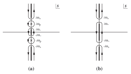
Figure 3.1: The analytic structure of the fermion propagator $S(s,\mathbf{k})$ and the complex contour used for evaluating the mean field $\psi(\mathbf{k},t)$ for (a) $m<2M$ and (b) $m>2M$.

On the other hand, for $m>2M$ (i.e., when the scalar particle can decay into fermion pairs) the fermion poles become complex and are embedded in the lower cut, and one must find out if they are complex poles in the physical sheet (the domain of integration) or moves off to the unphysical (second) sheet.

3.3.1 Complex poles or resonances

For $m>2M$ the fermion poles become complex and are embedded in the cut $s=-i\omega$ with $|\omega|<\omega_{-}(k)$. The position of the complex poles are determined from the zeros of $\omega^{2}-\bar{\omega}^{2}_{\mathbf{k}}-\Pi(\omega,\mathbf{k})$ in the denominator of the analytically continued fermion propagator for $\omega=\omega_{\mathrm{p}}(k)-i\gamma(k)$, where $\omega_{\mathrm{p}}(k)$ [$\gamma(k)$] is the real (imaginary) part of the complex pole. In the following discussion, we consider the narrow width approximation, $|\gamma(k)/\omega_{\mathrm{p}}(k)|\ll 1$, where the physical concept of a propagating mode is still meaningful.

With the expressions for the discontinuities in the physical sheet given by Eq. (3.25), the position of the complex pole is determined by

$$[\omega_{\mathrm{p}}(k)-i\gamma(k)]^{2}-\bar{\omega}^{2}_{\mathbf{k}}-\mathrm{Re}\Pi(\omega_{\mathrm{p}}(k),\mathbf{k})+i\,\mathrm{sgn}[\gamma(k)]\,\mathrm{Im}\Pi(\omega_{\mathrm{p}}(k),\mathbf{k})=0.$$ (3.34)

Retaining terms at most linear in $\gamma(k)$, one finds the real and imaginary parts of Eq. (3.34), respectively, become

$$\omega^{2}_{\mathrm{p}}(k)=\bar{\omega}^{2}_{\mathbf{k}}+\mathrm{Re}\Pi(\omega_{\mathrm{p}}(k),\mathbf{k}),$$ (3.35)

and

$$\gamma(k)=\mathrm{sgn}[\gamma(k)]\,\frac{\mathrm{Im}\Pi(\omega_{\mathrm{p}}(k),\mathbf{k})}{2\omega_{\mathrm{p}}(k)}.$$ (3.36)

Since $\mathrm{Re}\Pi(\omega,\mathbf{k})$ is an even function of $\omega$, here and henceforth, we choose $\omega_{\mathrm{p}}(k)$ to be the positive solution of Eq. (3.35). To lowest order, one finds

$$\omega_{\mathrm{p}}(k) = \bar{\omega}_{\mathbf{k}}+\frac{\mathrm{Re}\Pi(\bar{\omega}_{\mathbf{k}},\mathbf{k})}{2\bar{\omega}_{\mathbf{k}}}$$ (3.37)

$$= \bar{\omega}_{\mathbf{k}}+\frac{1}{4\bar{\omega}_{\mathbf{k}}}\mathrm{Tr}[(\gamma^{0}\omega_{\mathbf{k}}-\boldsymbol{\gamma}\cdot\mathbf{k}+M)\,\mathrm{Re}\Sigma(\bar{\omega}_{\mathbf{k}},\mathbf{k})].$$

To this order, the solution for $\gamma(k)$ is obtained by approximating $\omega_{\mathrm{p}}(k)\approx\bar{\omega}_{\mathbf{k}}$ in Eq. (3.36).

A close inspection, however, shows that Eq. (3.36) cannot have a solution because $\mathrm{Im}\Pi(\omega,\mathbf{k})$ is an odd function of $\omega$ and $\mathrm{Im}\Pi(\bar{\omega}_{\mathbf{k}},\mathbf{k})<0$. Therefore, there is no complex pole in the physical sheet. Indeed, this is a fairly well-known (but seldom noticed) result: if the imaginary part of the self-energy on the mass shell is negative, then there is no complex pole in the physical sheet and the pole has moved off into the unphysical (second) sheet.

In the case that $\mathrm{Im}\Pi(\bar{\omega}_{\mathbf{k}},\mathbf{k})>0$, complex poles appear in the physical sheet, but in such case there are two poles with both signs for $\gamma(k)$ (one corresponds to a decaying exponential in time and the other a growing exponential in time), which is the signal of an instability, not of damping. However since we confirm that $\mathrm{Im}\Pi(\bar{\omega}_{\mathbf{k}},\mathbf{k})$ is negative in the case under consideration, the complex poles are in the unphysical sheet and correspond to resonances.

3.3.2 Scalar decay implies fermion damping

We have shown that there are no complex poles in the physical sheet in the complex $s$-plane (the integration region), hence the only singularities are the cuts along the imaginary axis $s=-i\omega$ with $|\omega|<\omega_{-}(k)$ and $|\omega|>\omega_{+}(k)$. The contour of integration can be deformed to wrap around these cuts as depicted in Fig. 3.1 (b). Since the resonance is below (and away from) the multiparticle cut $|\omega|>\omega_{+}(k)$, in the narrow width approximation and consistent with perturbation theory the contribution from the cut $|\omega|<\omega_{-}(k)$ becomes the dominant one while that from the multiparticle cut is always perturbatively small.

It proves convenient to write the product in Eq. (3.20) in the compact form

$$S(s,\mathbf{k})\left[\boldsymbol{\gamma}\cdot\mathbf{k}+M+\widetilde{\Sigma}(0,\mathbf{k})\right]=\frac{\mathcal{N}(s,k)}{-s^{2}-\bar{\omega}^{2}_{\mathbf{k}}-\Pi(s,k)},$$ (3.38)

which defines $\mathcal{N}(s,k)$, and to change variables to $s=-i\omega\pm 0^{+}$ on the right-hand ($+$) and left-hand ($-$) side of the cut. After some algebra, one finds the following contribution to the real time evolution of the mean field

$$\psi(\mathbf{k},t) = \frac{1}{\pi}\int_{-\omega_{-}}^{+\omega_{-}}\frac{d\omega}{\omega}\,e^{-i\omega t}\left[\frac{\mathrm{Re}\mathcal{N}(\omega,\mathbf{k})\,\mathrm{Im}\Pi(\omega,\mathbf{k})}{[\omega^{2}-\bar{\omega}^{2}_{\mathbf{k}}-\mathrm{Re}\Pi(\omega,\mathbf{k})]^{2}+\mathrm{Im}\Pi(\omega,\mathbf{k})^{2}}\right.$$ (3.39)

$$+\left.\frac{\mathrm{Im}\mathcal{N}(\omega,\mathbf{k})[\omega^{2}-\bar{\omega}^{2}_{\mathbf{k}}-\mathrm{Re}\Pi(\omega,\mathbf{k})]}{[\omega^{2}-\bar{\omega}^{2}_{\mathbf{k}}-\mathrm{Re}\Pi(\omega,\mathbf{k})]^{2}+\mathrm{Im}\Pi(\omega,\mathbf{k})^{2}}\right]\psi(\mathbf{k},0).$$

The term proportional to $\mathrm{Re}\mathcal{N}(\omega,\mathbf{k})$ features a typical Breit-Wigner resonance near the real part of the complex pole, where $\omega^{2}_{\mathrm{p}}-\bar{\omega}^{2}_{\mathbf{k}}-\Pi_{R}(\omega_{\mathrm{p}},\mathbf{k})=0$, since, for $m>2M$, the imaginary part of the self-energy at this value of $\omega$ (perturbatively close to $\pm\omega_{\mathbf{k}}$) is nonvanishing. On the other hand, the term proportional to $\mathrm{Im}\mathcal{N}(\omega,\mathbf{k})$ is a representation of the principal part in the limit of small $\mathrm{Re}\Pi(\omega,\mathbf{k})$ and is therefore subleading.

The sharply peaked resonances at $\omega=\pm\omega_{\mathrm{p}}(k)$ dominate the integral and give the largest contribution to the real-time evolution of $\psi(\mathbf{k},t)$. In the limit of a narrow resonance, the $\omega$ integral is performed by taking the integration limits to infinity and approximating near the resonances at $\omega=\pm\omega_{\mathrm{p}}(k)$

$$-\frac{1}{\omega}\frac{\mathrm{Im}\Pi(\omega,\mathbf{k})}{[\omega^{2}-\bar{\omega}^{2}_{\mathbf{k}}-\mathrm{Re}\Pi(\omega,\mathbf{k})]^{2}+\mathrm{Im}\Pi(\omega,\mathbf{k})^{2}}\approx\frac{Z(k)}{2\,\omega^{2}_{\mathrm{p}}(k)}\,\frac{\gamma(k)}{[\omega\mp\omega_{\mathrm{p}}(k)]^{2}+\gamma^{2}(k)},$$ (3.40)

where

$$Z(k)=\left[1-\frac{\partial\mathrm{Re}\Pi(\omega,\mathbf{k})}{\partial\omega^{2}}\right]_{\omega=\omega_{\mathrm{p}}(k)}^{-1},\qquad\gamma(k)=-\frac{Z(k)}{2\omega_{\mathrm{p}}(k)}\mathrm{Im}\Pi(\omega_{\mathrm{p}}(k),\mathbf{k}).$$ (3.41)

The wave function renormalization constant $Z(k)$ is finite, since the effective self-energy $\Pi(\omega,\mathbf{k})$ has been rendered finite by an appropriate choice of counterterms. Only when the counterterms are chosen to provide a subtraction of the self-energy at the position of the resonance $\omega\approx\pm\omega_{\mathrm{p}}(k)$ will result in $Z(k)=1$. On the other hand, as noted above, if the counterterms are chosen to renormalize the theory on the fermion mass shell at zero temperature then $Z(k)$ describes the dressing of the medium and is smaller than one. As will be shown shortly, the width of the Breit-Wigner resonance $\gamma(k)$ is the damping rate of the fermion mean field.

The integration in the variable $\omega$ can be performed under these approximations (justified for narrow width), leading to the real-time evolution

$$\psi(\mathbf{k},t)\approx\frac{Z(k)}{2\omega^{2}_{\mathrm{p}}(k)}\left[\mathrm{Re}\mathcal{N}(\omega_{\mathrm{p}}(k),\mathbf{k})\,e^{-i\omega_{\mathrm{p}}(k)t}+\mathrm{Re}\mathcal{N}(-\omega_{\mathrm{p}}(k),\mathbf{k})\,e^{i\omega_{\mathrm{p}}(k)t}\right]\,e^{-\gamma(k)t}\,\psi(\mathbf{k},0).$$ (3.42)

Gathering the results for $\mathrm{Im}\Pi(\bar{\omega}_{\mathrm{p}}(k),\mathbf{k})$ given in Eq. (3.32), we find the damping rate for the fermion mean fields at one-loop order to be given by (for $m>2M$)

$$\gamma(k)=\frac{y^{2}m^{2}T}{32\pi k\bar{\omega}_{\mathbf{k}}}\left(1-\frac{4M^{2}}{m^{2}}\right)\ln\left.\left[\frac{1-e^{-\beta(\bar{\omega}_{\mathbf{q}}+\bar{\omega}_{\mathbf{k}})}}{1+e^{-\beta\bar{\omega}_{\mathbf{q}}}}\right]\right|^{q=q^{+}}_{q=q^{-}},$$ (3.43)

where $q^{\pm}$ are given in Eq. (3.33).

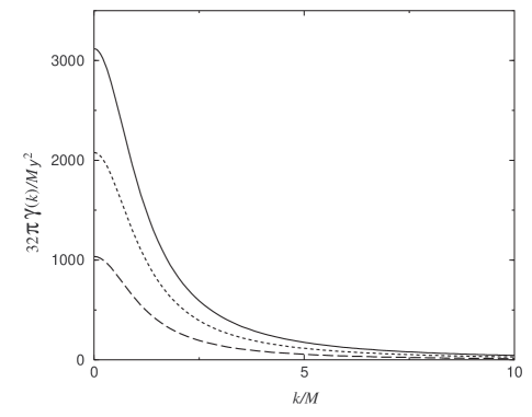
Figure 3.2: The fermion damping rate plotted as a function of the momentum for $m/M=4$ and $T/M=150$ (solid), 100 (dotted), and 50 (dashed).

Figures 3.2 and 3.3 display the behavior of $\gamma(k)$ for several ranges of the parameters. We have chosen a wide range of parameters for the ratios of the scalar to fermion masses ($m/M$) and the temperature to fermion mass ($T/M$) to illustrate in detail the important differences. The damping rate features a strong peak as a function of the ratio $k/M$. This peak is at very small momentum when the ratio of scalar to fermion mass is not much larger than 2, but moves to larger values of the fermion momentum when this ratio is very large. Figure 3.3 displays this feature in an extreme case ($m/M=800$) to highlight this behavior. The height of the peak is a monotonically increasing function of temperature as expected. This is one of the important results of this work: the decay of the heavy scalar into fermion pairs results in a induced damping of the amplitude of fermionic excitations.

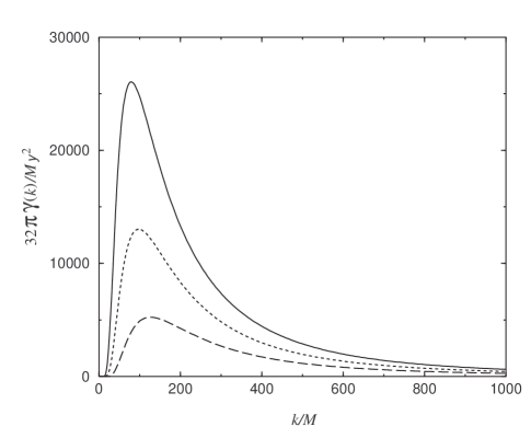
Figure 3.3: The fermion damping rate plotted as a function of the momentum for $m/M=800$ and $T/M=1000$ (solid), 800 (dotted), and 600 (dashed).

3.3.3 All-order expression for the damping rate

Since there is no complex pole solution in the physical sheet for $m>2M$, there are no solutions of the effective in-medium Dirac equation. However, we can define the spinor wave function of the resonance by considering the solutions of the in-medium Dirac equation with only the real part of the self-energy at $\omega=\pm\omega_{\mathrm{p}}(k)$ [59, 60]. The form given by Eq. (3.19) for the self-energy is general and not restricted to perturbation theory, hence our analysis below is valid to all orders in perturbation theory.

Using the expression for the self-energy given by Eq. (3.19) for $s=\mp i\omega_{\mathrm{p}}(k)+0^{+}$, and introducing the following variables

$$\mathcal{W} = \omega_{\mathrm{p}}(k)\,[1-\mathrm{Re}\mathcal{E}^{(0)}(\omega_{\mathrm{p}}(k),\mathbf{k})],$$

$$\boldsymbol{\mathcal{K}} = \mathbf{k}\,[1+\mathrm{Re}\mathcal{E}^{(1)}(\omega_{\mathrm{p}}(k),\mathbf{k})],$$

$$\mathcal{M} = M\,[1+\mathrm{Re}\mathcal{E}^{(2)}(\omega_{\mathrm{p}}(k),\mathbf{k})],$$ (3.44)

we find the resonance wave functions $\Psi_{s}(\pm\omega_{\mathrm{p}}(k),\mathbf{k})$ obey the following effective in-medium Dirac equation

$$\left(\pm\gamma^{0}\mathcal{W}-\boldsymbol{\gamma}\cdot\boldsymbol{\mathcal{K}}-\mathcal{M}\right)\Psi_{s}(\pm\omega_{\mathrm{p}}(k),\mathbf{k})=0,$$ (3.45)

where $s=1,2$ labels the spin. Furthermore, using the properties that $\mathrm{Re}\,\mathcal{E}^{(i)}(\omega,\mathbf{k})$ are even functions of $\omega$ and depend on $k$, we can define two in-medium particle (i.e., positive energy) solutions $U_{s}(\mathbf{k})=\Psi_{s}(\omega_{\mathrm{p}}(k),\mathbf{k})$ and two in-medium antiparticle (i.e., negative energy) solutions $V_{s}(\mathbf{k})=\Psi_{s}(-\omega_{\mathrm{p}}(k),-\mathbf{k})$. These in-medium Dirac spinors satisfy

$$\left(\gamma^{0}\mathcal{W}-\boldsymbol{\gamma}\cdot\boldsymbol{\mathcal{K}}-\mathcal{M}\right)\,U_{s}(\mathbf{k})=0,$$

$$\left(\gamma^{0}\mathcal{W}-\boldsymbol{\gamma}\cdot\boldsymbol{\mathcal{K}}+\mathcal{M}\right)\,V_{s}(\mathbf{k})=0,$$ (3.46)

and can be constructed from the usual free Dirac spinors through the replacement $\bar{\omega}_{\mathbf{k}}\rightarrow\mathcal{W}$, $\mathbf{k}\rightarrow\boldsymbol{\mathcal{K}}$, and $M\rightarrow\mathcal{M}$.

Combining Eqs. (3.19), (3.25) and (3.29), we obtain, from the definition of the damping rate given by Eq. (3.40), the following expression for the width of the resonance to all orders in perturbation theory:

$$\gamma(k) = -\frac{Z(k)}{4\,\omega_{\mathrm{p}}(k)}\mathrm{Tr}\left[(\gamma^{0}\mathcal{W}-\boldsymbol{\gamma}\cdot\boldsymbol{\mathcal{K}}+\mathcal{M})\,\mathrm{Im}\Sigma(\omega_{\mathrm{p}}(k),\mathbf{k})\right]$$ (3.47)

$$= -\frac{\mathcal{M}Z(k)}{2\,\omega_{\mathrm{p}}(k)}\sum_{s=1,2}\left[\bar{U}_{s}(\mathbf{k})\,\mathrm{Im}\Sigma(\omega_{\mathrm{p}}(k),\mathbf{k})\,U_{s}(\mathbf{k})\right],$$

where we have alternatively written the expression for the width in terms of the exact resonance spinors in the medium. This result confirms those found in Refs. [59, 60] and leads to the often quoted expression for the width in lowest order [54, 43].

3.4 Kinetics of Fermion Relaxation

To clarify and confirm independently the result of the previous section that decay of the scalar leads to a quasiparticle width of the fermionic excitations, we now provide an analysis of the relaxation of the fermion distribution function via a kinetic Boltzmann equation. This analysis will also provide, directly in real time, a firm relationship between the damping rate and the interaction rate in the relaxation time approximation (i.e., linearization near equilibrium).

Because here we are only interested in the kinetics of fermions, we assume that the scalars are in thermal equilibrium. Let us denote the distribution function for fermions of momentum $\mathbf{k}$ and spin $s$ by $\bar{n}_{s,\mathbf{k}}(t)$. In the kinetic approach, the time derivative of this distribution function is obtained from the Boltzmann equation. Since for a fixed spin component the matrix elements for the transition probabilities are rather cumbersome, we study the spin-averaged fermion distribution function defined as $\bar{n}_{\mathbf{k}}(t)=\frac{1}{2}\sum_{s}\bar{n}_{\mathbf{k},s}(t)$.

For $m>2M$, two processes are responsible for the change in the fermion populations in a fermion-scalar plasma: $s\rightarrow f+\bar{f}$, which provides the “gain” term in the balance equation, and $f+\bar{f}\rightarrow s$, which provides the “loss” term. Using the standard approach to obtain the semiclassical Boltzmann equation, we find

$$\frac{d}{dt}\bar{n}_{\mathbf{k}}(t) = \pi y^{2}\int\frac{d^{3}q}{(2\pi)^{3}}\frac{\bar{\omega}_{\mathbf{k}}\bar{\omega}_{\mathbf{q}}-\mathbf{k}\cdot\mathbf{q}-M^{2}}{2\bar{\omega}_{\mathbf{q}}\bar{\omega}_{\mathbf{k}}\omega_{\mathbf{p}}}\,\delta(\bar{\omega}_{\mathbf{k}}+\bar{\omega}_{\mathbf{q}}-\omega_{\mathbf{p}})$$ (3.48)

$$\times\left[n_{B}(\omega_{\mathbf{p}})[1-\bar{n}_{\mathbf{k}}(t)][1-\bar{n}_{\mathbf{q}}(t)]-[1+n_{B}(\omega_{\mathbf{p}})]\bar{n}_{\mathbf{k}}(t)\bar{n}_{\mathbf{q}}(t)\right],$$

where $\mathbf{p=k+q}$. It is easy to check that the above equation has an equilibrium solution given by $\bar{n}_{\mathbf{k}}(t)=n_{F}(\bar{\omega}_{\mathbf{k}})$ for all momentum $\mathbf{k}$.

Let us now consider small departure for fermions from this equilibrium solution and study the relaxation to equilibrium in the relaxation time approximation. This is achieved by introducing a disturbance in the distribution function for fermion of (fixed) momentum $\mathbf{k}$ so that

$$\bar{n}_{\mathbf{k}}(t)=n_{F}(\bar{\omega}_{\mathbf{k}})+\delta\bar{n}_{\mathbf{k}}(t),$$ (3.49)

where $\delta\bar{n}_{\mathbf{k}}(t)/n_{F}(\bar{\omega}_{\mathbf{k}})\ll 1$. Retaining terms at most linear in $\delta\bar{n}_{\mathbf{k}}(t)$, one obtains from Eq. (3.48) an equation for $\delta\bar{n}_{\mathbf{k}}(t)$

$$\frac{d}{dt}\,\delta\bar{n}_{\mathbf{k}}(t)=-\Gamma(k)\,\delta\bar{n}_{\mathbf{k}}(t),$$ (3.50)

where $\Gamma(k)$ is the interaction rate, whose inverse characterizes the time scale for the fermion distribution to approach equilibrium [54]

$$\Gamma(k) = \pi y^{2}\int\frac{d^{3}q}{(2\pi)^{3}}\frac{\bar{\omega}_{\mathbf{k}}\bar{\omega}_{\mathbf{q}}-\mathbf{k}\cdot\mathbf{q}-M^{2}}{2\bar{\omega}_{\mathbf{k}}\bar{\omega}_{\mathbf{q}}\omega_{\mathbf{p}}}\,[n_{B}(\omega_{\mathbf{p}})+n_{F}(\bar{\omega}_{\mathbf{q}})]\,\delta(\bar{\omega}_{\mathbf{k}}-\omega_{\mathbf{p}}+\bar{\omega}_{\mathbf{q}})$$ (3.51)

$$= \frac{y^{2}m^{2}T}{16\pi k\bar{\omega}_{\mathbf{k}}}\left(1-\frac{4M^{2}}{m^{2}}\right)\ln\left.\left[\frac{1-e^{-\beta(\bar{\omega}_{\mathbf{q}}+\bar{\omega}_{\mathbf{k}})}}{1+e^{-\beta\bar{\omega}_{\mathbf{q}}}}\right]\right|^{q=q^{+}}_{q=q^{-}},$$

with $q^{\pm}$ given in Eq. (3.33).

Upon comparing the interaction rate with the damping rate found in the previous section [see Eq. (3.43)], we provide a real-time confirmation of the result

$$\Gamma(k)=2\,\gamma(k).$$ (3.52)

The kinetic analysis confirms that the damping of the fermionic quasiparticle excitations in the medium is a consequence of the decay of the heavy scalar. Furthermore, this analysis is carried out directly in real time and clearly establishes the relation between the interaction rate in the relaxation time approximation and the damping rate of the mean field at least to lowest order.

Recently a detailed investigation between the damping and interaction rates for chiral fermions in gauge theories at finite temperature has been reported in Ref. [61] within the framework of the imaginary-time (Matsubara) formalism of finite-temperature field theory. Our analysis provides a complementary confirmation of this result in real time both for the relaxation of the mean field and that of the spin-averaged fermion distribution function.

3.5 Conclusions

In this chapter we have focused on studying the propagation of fermion excitations in a fermion-scalar plasma, as a complement to the more studied issue of fermion propagation in a hot (Abelian or non-Abelian) plasma. Our motivation was to provide a real-time analysis of the propagation of fermions that could eventually be used in other problems such as neutrino oscillations in the medium and nonequilibrium processes in electroweak baryogenesis.

The first step of the program is to obtain the effective in-medium Dirac equation for the fermion mean field directly in real time. This is achieved by relating the problem of linear response to an initial value problem for the fermion mean field induced by an external Grassmann source that is adiabatically switched on from remote past and switched off at time $t=0$. The resulting effective Dirac equation for the mean field is fully renormalized, retarded and causal, thus allowing a direct study of real-time relaxation of the mean field. We study in detail the structure of the renormalized fermion self-energy and establish the presence of new cuts of thermal origin in the fermion propagator. We found that when the scalar mass is large enough that decay of the scalar into fermion pairs is kinematically allowed, this decay process results in an induced damping of the fermion excitations and their propagation in the medium as quasiparticle resonances. Solving the effective Dirac equation by Laplace transform, we obtained the time evolution of the fermion mean field, which leads to a clear identification of the damping rate. We calculate the damping rate in the narrow width approximation to one loop order for arbitrary values of the fermion and scalar masses (provided the scalar is heavy enough to decay), temperature and fermion momentum.

An all-order expression for the fermion damping rate (in the narrow width approximation) is obtained from an analysis of the structure of the self-energy and the exact quasiparticle spinor wave functions. A kinetic approach based on a semiclassical Boltzmann kinetic equation for the spin-averaged fermion distribution function reveals that the interaction rate (obtained in the relaxation time approximation) is twice the damping rate of the mean fields at least to lowest order in the Yukawa coupling. We emphasize that this relation is established from a real-time analysis both for the mean field and the distribution function.

Although the expression for the damping rate was obtained for arbitrary values of the scalar and fermion masses, temperature and fermion momentum, a deeper analysis is required if the theory undergoes a second-order (or weakly first-order) phase transition. The reason being that if the fermion masses are a result of spontaneous symmetry breaking in the scalar sector, near a second-order (or weak first-order) phase transition both the scalar mass and the chiral breaking fermion mass vanish. In this case the kinematic region in momentum space for which the energy conservation delta functions are fulfilled shrinks and one must understand if, for soft fermion momentum $k\sim yT$, a resummation akin to the hard thermal loops (HTL’s) [62] in hot gauge field theory is required [63].

Chapter 4 Dynamical Renormalization Group Approach to Quantum Kinetics

4.1 Introduction

The ultrarelativistic heavy ion experiments at the BNL Relativistic Heavy Ion Collider (RHIC) and the forthcoming CERN Large Hadron Collider (LHC) have the potential of providing clear evidence for the formation of the quark-gluon plasma (QGP) [2, 3] and hopefully to study the chiral phase transition [14]. Since this is perhaps the only opportunity to study phase transitions that are conjectured to occur in particle physics with earth-bound accelerators, a great theoretical effort parallel to the experimental work has been devoted to understanding the signatures of the QGP and the chiral phase transition.

A essential part of this theoretical program is to establish, from first principles, a consistent quantum kinetic description of transport phenomena in a hot nonequilibrium multiparton system. Such a kinetic description has the potential of providing a detailed understanding of experimental signatures such as photon and dilepton production, charmonium suppression, strangeness enhancement, freeze-out of hadrons, and collective flow [64, 65] that will lead to an unambiguous determination of the formation of the QGP and the observables of chiral phase transitions in ultrarelativistic heavy ion collisions. The kinetic description is also of fundamental importance in the understanding of the emergence of hydrodynamics in the long-wavelength limit of quantum field theories [66]. During the last few years, there have been significant advances ranging from first-principle derivations of kinetic and transport equations in QCD [67, 68, 49, 48] and scalar field theories [69, 70, 71, 72, 73], numerical codes that describe the space-time evolution of heavy ion collisions such as the screened perturbative QCD (pQCD) parton model [6, 74], the parton cascade model [7] and the hydrodynamical transport model [8] to lattice simulations of nonequilibrium dynamics in quantum field theories [75, 76] and classical gauge theories [77, 78, 79]. Furthermore, an effective quantum kinetic equation has been advocated as a description of the dynamics of soft collective excitations in hot non-Abelian plasmas [80, 81, 82, 83, 48].

The typical approach to derive quantum kinetic equation involves a Wigner transform of the two-point Green’s functions and a gradient expansion [49, 48, 67, 68, 85] (a gauge covariant Wigner transform in the case of gauge theories) and often requires a quasiparticle approximation [48, 68, 73, 85]. The gradient expansion assumes that the center-of-mass Wigner variables are slowly varying, but it is seldom clear at this level which are the fast and which are the slow scales involved. A “coarse-graining” procedure is typically invoked that averages out microscopic scales in the kinetic description, leading to irreversible evolution in the resulting kinetic equation. Such an averaging procedure is usually poorly understood and justified a posteriori. The quasiparticle approximation consists in neglecting the broadening of the single-particle states when computing the collision terms. A derivation of quantum kinetic equation for a hot QCD plasma along these lines has recently been reported recently in Ref. [48], however the collision terms obtained in the quasiparticle approximation turn out to be infrared divergent.

The goal of this chapter is to provide a novel and alternative derivation of quantum kinetic equations directly in real time from the underlying quantum field theory by implementing a dynamical renormalization group (DRG) resummation. The strategy to be followed is a generalization of the dynamical renormalization group method introduced in Ref. [84] to study anomalous relaxation in Abelian gauge theories, but adapted to the description of quantum kinetics [71, 86]. The starting point is the identification of the distribution function of the quasiparticles which could require a resummation of medium effects (the equivalent of hard thermal loops [62]). The equation of motion for this distribution function is solved in a perturbative expansion in terms of nonequilibrium Feynman diagrams. The perturbative solution in real time gives rise secular terms that grow rapidly with time and invalidate the perturbative expansion beyond a particular time scale (recognized a posteriori as the kinetic time scale). The dynamical renormalization group implements a systematic resummation of these secular terms and the resulting renormalization group equation is the quantum kinetic equation.

The validity of this approach hinges upon the basic assumption of a wide separation between the microscopic and the kinetic time scales. Such an assumption underlies every approach to a kinetic description and is generally justified in weakly coupled theories. Unlike other approaches in terms of a truncation of the equations of motion for the Wigner distribution function, the main ingredient in the approach presented here is a perturbative diagrammatic evaluation of the time evolution of the distribution function in real time [71] improved via a renormalization group resummation of the secular divergences.

An important bonus of this approach is that it illuminates the origin and provides a natural resolution of pinch singularities [87, 88] found in perturbation theory out of equilibrium. The perturbative real-time approach combined with the renormalization group resummation reveal clearly that these are indicative of the nonequilibrium evolution of the distribution functions. In this framework, pinch singularities are the manifestation of secular terms.

This chapter is organized as follows. In Sec. 4.2 we study in detail the dynamical renormalization group approach to quantum kinetics in the familiar case of a self-interacting scalar theory, including in addition a nonequilibrium resummation akin to the hard thermal loops to account for the effective scalar masses in the medium and therefore the relevant microscopic time scales. In Sec. 4.3 we discuss the main features of the dynamical renormalization group method and compare it to the more familiar renormalization group in Euclidean field theory.

In Sec. 4.4 we apply these techniques to obtain the kinetic equations for pions and sigma mesons in the $O(4)$ linear sigma model in the chiral limit. In relaxation time approximation we obtain the relaxation rates for pions and sigma mesons. This case allows us to highlight the power of this the dynamical renormalization group approach to study threshold effects on the relaxation of resonances, in particular the crossover between two different relaxation regimes as a function of the momentum of the resonance. This aspect becomes phenomenological important in view of the recent studies by Hatsuda et al. [89] that reveal a dropping of the sigma mass near the chiral phase transition and an enhancement of threshold effects with potential observational consequences in ultrarelativistic heavy ion collisions. In Sec. 4.5 we discuss the issue of pinch singularities found in calculations in the so-called real-time formalism of nonequilibrium field theory and provide a resolution via the dynamical renormalization group. In Sec. 4.6 we summarize our results and discuss further implications.

4.2 Self-Interacting Scalar Theory

The starting point is the following Lagrangian for a hot scalar theory:

$${\cal{L}}[\phi]=\frac{1}{2}\left(\partial_{\mu}\phi\right)^{2}-\frac{1}{2}m^{2}\phi^{2}-\frac{\lambda}{4!}\phi^{4},$$ (4.1)

where $m$ and $\lambda$ are the physical parameters defined in the vacuum (or, at zero temperature). Since we focus on medium (finite-temperature) effects, in the following discussion we ignore the vacuum (zero-temperature) ultraviolet divergences that can be absorbed into the renormalization of $m$ and $\lambda$.

The first step towards understanding the kinetic regime is the identification of the microscopic time scales in the problem. In the medium, the bare particles are dressed by the interactions becoming “quasiparticles”. One is interested in describing the relaxation of these quasiparticles. Thus the important microscopic time scales are those associated with the quasiparticles and not the bare particles. If a kinetic equation is obtained in some perturbative scheme, such a scheme should be in terms of the quasiparticles, which already implies a resummation of the perturbative expansion accounting for the medium effects. This resummed perturbative expansion is precisely the rationale behind the hard thermal loop (HTL) program developed by Braaten and Pisarski [62] in hot gauge field theory and also behind the self-consistent treatment in nonequilibrium scalar field theory proposed by Lawrie [70].

Since we are interested in obtaining a kinetic equation for the quasiparticle distribution function, the most natural initial state corresponds to an initial density matrix $\rho$ prepared at time $t=t_{0}$ that is diagonal in the basis of free quasiparticles number operator (defined below) but with nonequilibrium quasiparticle distribution functions $n_{\mathbf{k}}(t_{0})$ (see Sec. 2.2). In this picture the width of the quasiparticles arises from their interaction and is related to the relaxation rate of the distribution function in the relaxation time approximation. This point will become more clear below.

With such a choice of initial density matrix, perturbative expansions are carried out with the following nonequilibrium free quasiparticle Wightman functions (in momentum space):

$$G_{0}^{>}(\mathbf{k},t,t^{\prime}) = \frac{i}{2\omega_{\mathbf{k}}}\left[[1+n_{\mathbf{k}}(t_{0})]\,e^{-i\omega_{\mathbf{k}}(t-t^{\prime})}+n_{\mathbf{k}}(t_{0})\,e^{i\omega_{\mathbf{k}}(t-t^{\prime})}\right],$$

$$G_{0}^{<}(\mathbf{k},t,t^{\prime}) = \frac{i}{2\omega_{\mathbf{k}}}\left[n_{\mathbf{k}}(t_{0})\,e^{-i\omega_{\mathbf{k}}(t-t^{\prime})}+[1+n_{\mathbf{k}}(t_{0})]\,e^{i\omega_{\mathbf{k}}(t-t^{\prime})}\right],$$ (4.2)

where $\omega_{\mathbf{k}}=\sqrt{\mathbf{k}^{2}+m^{2}_{\mathrm{eff}}}$ is the energy of the free quasiparticle and $m_{\mathrm{eff}}$ is the quasiparticle effective mass to be determined self-consistently below. We note that it is easy to check the relation

$$G_{0}^{>}(\mathbf{k},t,t^{\prime})=G_{0}^{<}(\mathbf{k},t^{\prime},t),$$ (4.3)

which will be useful in following calculations.

In the self-interacting scalar field theory the HTL resummation can be implemented by writing $m$ in the Lagrangian as

$$m^{2}=m^{2}_{\mathrm{eff}}+\delta m^{2},$$ (4.4)

where $m_{\mathrm{eff}}$ is the effective quasiparticle mass which enters in the effective propagators for free quasiparticles [see Eq. (4.2)], and $\delta m^{2}$ is a counter term which will cancel a subset of Feynman diagrams in the perturbative expansion and is considered part of the interaction Lagrangian. The effective mass $m_{\mathrm{eff}}$ will in general depend on the state of the system (e.g., distribution functions of the scalars) through the medium effects. In particular, in thermal equilibrium $m_{\mathrm{eff}}$ depends on the temperature and is called the thermal mass [43].

We note that one could also introduce counter term for the coupling constant and proceed with a resummed perturbative expansion in terms of the in-medium effective propagators and vertices, akin to those in the HTL program for hot gauge theory [62, 43]. However, to lowest order that we are interested in only the mass counter term is relevant.

The implementation of this resummation scheme to lowest in perturbation theory is achieved by requiring that the mass counter term $\delta m^{2}$ cancel the one-loop tadpole contribution to the scalar self-energy [90]. This leads to the following self-consistent gap equation for $m^{2}_{\mathrm{eff}}$ [71]

$$m^{2}_{\mathrm{eff}}=m^{2}+\frac{\lambda}{2}\int\frac{d^{3}k}{(2\pi)^{3}}\frac{n_{\mathbf{k}}(t_{0})}{\sqrt{k^{2}+m^{2}_{\mathrm{eff}}}},$$ (4.5)

where $n_{\mathbf{k}}(t_{0})$ is the initial (nonequilibrium) distribution of the quasiparticles at time $t=t_{0}$. We emphasize that $m_{\mathrm{eff}}$ depends on the initial quasiparticle distribution functions. This observation will become important later when we discuss the time evolution of the quasiparticle distribution functions and therefore of the effective mass.

Assuming that the system is in thermal equilibrium, one can make an assessment of the (thermal) effective mass $m_{\mathrm{eff}}(T)$. Upon substituting the replacement of equilibrium distribution functions $n_{\mathbf{k}}(t_{0})\rightarrow n_{B}(\sqrt{k^{2}+m^{2}_{\mathrm{eff}}(T)})$ in Eq. (4.5), one finds that for $T\gg m_{\mathrm{eff}}(T)$ the solution of the gap equation is given by [90, 91]

$$m^{2}_{\mathrm{eff}}(T)=m^{2}+\frac{\lambda}{2}\left[\frac{T^{2}}{12}-\frac{T}{4\pi}m_{\mathrm{eff}}(T)+\mathcal{O}\left(m^{2}_{\mathrm{eff}}(T)\,\ln\frac{m_{\mathrm{eff}}(T)}{T}\right)\right].$$ (4.6)

In particular, for $T\gg\sqrt{\lambda}\,T\gg m$ (justified in the weak coupling limit), one can neglect the mass $m$ and obtains

$$m^{2}_{\mathrm{eff}}(T)=\frac{\lambda\,T^{2}}{24}\left[1+\mathcal{O}(\lambda^{1/2})\right].$$ (4.7)

We note that this effective mass determines the important time scales in the medium but is not the position of the quasiparticle pole (or, strictly speaking, resonance).

In the massless case, $m_{\mathrm{eff}}(T)$ serves as an infrared cutoff for the loop integrals [90, 92], hence the leading term of Eq. (4.7) provides the correct microscopic time scale at high temperature. Furthermore, when the temperature is much larger than the vacuum (zero temperature) mass $m$, the self-consistent resummation is needed to incorporate the physically relevant microscopic time and length scales in the perturbative expansion, which, in the weakly coupling limit, is given by $t_{\mathrm{mic}}\sim 1/m_{\mathrm{eff}}(T)\sim 1/\sqrt{\lambda}T$.

4.2.1 Quantum kinetic equation for quasiparticles

Having explained the notion of quasiparticles in the medium and the microscopic time scales associated with them, we now proceed to obtain the kinetic equation for the quasiparticle distribution functions. Here we present an alternative to the usual derivation in which correlation functions are written in terms of relative and center-of-mass space-time coordinates and a Wigner transform in the relative coordinates is performed. In this approach the kinetic equation is obtained in a gradient expansion assuming that the dependence on center-of-mass coordinates is weak. Here, however, we will not assume such a situation, but instead analyze which are the relevant time scales over which a coarse graining procedure must be implemented.

In the presence of the medium the quasiparticles will have an effective mass $m_{\mathrm{eff}}$ resulting from medium effects, much in the same manner as the temperature dependent thermal mass in the equilibrium situation discussed above. This effective mass $m_{\mathrm{eff}}$ will be very different from the vacuum mass $m$ and must be taken into account for the correct assessment of the microscopic time scales. In the kinetic approach, this is achieved by writing the Hamiltonian of the theory as $H=H_{0}+H_{\mathrm{int}}$, where

$$H_{0}=\frac{1}{2}\int d^{3}x\left[\Pi^{2}+({\bf\nabla}\phi)^{2}+m^{2}_{\mathrm{eff}}\phi^{2}\right],\quad H_{\mathrm{int}}=\int d^{3}x\left[\frac{\lambda}{4!}\,\phi^{4}+\frac{\delta m^{2}}{2}\phi^{2}\right],$$ (4.8)

with $\Pi(\mathbf{x},t)=\partial\phi(\mathbf{x},t)/\partial t$ being the conjugate momentum of $\phi(\mathbf{x},t)$. In the above definition, the free Hamiltonian $H_{0}$ describes free quasiparticles of effective mass $m_{\mathrm{eff}}$ and is diagonal in terms of free quasiparticle creation and annihilation of operators $a^{\dagger}(\mathbf{k})$ and $a(\mathbf{k})$, respectively, and the mass counter term has been absorbed in the interaction Hamiltonian $H_{\mathrm{int}}$. The pole mass of the quasiparticles will acquire corrections in perturbation theory, but these will remain perturbatively. With this definition, the lifetime of the quasiparticles will be a consequence of interactions. In this manner, the nonequilibrium equivalent of the hard thermal loops (in the sense that the distribution functions are non-thermal), which in this theory amount to local (momentum independent) terms, have been absorbed in the definition of the effective mass. This guarantees that the microscopic time scales are explicit in the quasiparticle Hamiltonian.

As discussed above, we consider that the initial density matrix $\rho$ at time $t=t_{0}$ is diagonal in the basis of free quasiparticles number operator, but with nonequilibrium initial distribution functions $n_{\mathbf{k}}(t_{0})$. Hence, the Heisenberg quasiparticle field operators at time $t$ (in momentum space) can be written as

$$\phi(\mathbf{k},t)=\frac{1}{\sqrt{2\omega_{\mathbf{k}}}}\left[a(\mathbf{k},t)+a^{\dagger}(-\mathbf{k},t)\right],\quad\Pi(\mathbf{k},t)=i\sqrt{\frac{\omega_{\mathbf{k}}}{2}}\left[a^{\dagger}(-\mathbf{k},t)-a(\mathbf{k},t)\right],$$ (4.9)

where $a^{\dagger}(\mathbf{k},t)$ and $a(\mathbf{k},t)$, respectively, are the creation and annihilation operators in the Heisenberg picture and $\omega_{\mathbf{k}}=\sqrt{\mathbf{k}^{2}+m^{2}_{\mathrm{eff}}}$ as defined in Eq. (4.2) above. The expectation value of Heisenberg quasiparticle number operators $n_{\mathbf{k}}(t)$ is interpreted as the time dependent quasiparticle distribution function and can be expressed in terms of the field $\phi(\mathbf{k},t)$ and the conjugate momentum $\Pi(\mathbf{k},t)$ as follows

$$n_{\mathbf{k}}(t) = \langle a^{\dagger}(\mathbf{k},t)\,a(\mathbf{k},t)\rangle$$ (4.10)

$$= {1\over 2\omega_{\mathbf{k}}}\left[\left\langle\Pi(\mathbf{k},t)\,\Pi(-\mathbf{k},t)\right\rangle+\omega^{2}_{\mathbf{k}}\left\langle\phi(\mathbf{k},t)\,\phi(-\mathbf{k},t)\right\rangle\right]-\frac{1}{2},$$

where the bracket $\langle\,\cdot\,\rangle$ denotes the nonequilibrium expectation value with the initial (Gaussian) density matrix specified by the initial distribution functions $n_{\mathbf{k}}(t_{0})$.

The interaction Hamiltonian $H_{\mathrm{int}}$ in momentum space is given by

$$H_{\mathrm{int}} = \frac{\lambda}{4!}\int\prod_{i=1}^{4}\frac{d^{3}q_{i}}{(2\pi)^{3}}\,\phi({\mathbf{q}_{i}},t)\,(2\pi)^{3}\,\delta^{3}(\mathbf{q}_{1}+\mathbf{q}_{2}+\mathbf{q}_{3}+\mathbf{q}_{4})$$ (4.11)

$$+\,\frac{\delta m^{2}}{2}\int\frac{d^{3}q}{(2\pi)^{3}}\,\phi(\mathbf{q},t)\phi(-\mathbf{q},t).$$

Taking the derivative of $n_{\mathbf{k}}(t)$ with respect to time and using the Heisenberg field equations, one finds

$$\frac{d}{dt}n_{\mathbf{k}}(t) = -\frac{\lambda}{12\omega_{\mathbf{k}}}\,\Big{[}\left\langle[\phi^{3}(\mathbf{k},t)]\,\Pi(-\mathbf{k},t)\right\rangle+\left\langle\Pi(\mathbf{k},t)\,[\phi^{3}(\mathbf{k},t)]\right\rangle\Big{]}$$ (4.12)

$$+\,\frac{\delta m^{2}}{2\omega_{\mathbf{k}}}\,\Big{[}\left\langle\phi(\mathbf{k},t)\,\Pi(-\mathbf{k},t)\right\rangle+\left\langle\Pi(\mathbf{k},t)\,\phi(-\mathbf{k},t)\right\rangle\Big{]},$$

where we use the compact notation

$$[\phi^{3}(\mathbf{k},t)]\equiv\int\prod_{i=1}^{3}\frac{d^{3}q_{i}}{(2\pi)^{3}}\,\phi({\mathbf{q}_{i}},t)\,\delta^{3}(\mathbf{k}-\mathbf{q}_{1}-\mathbf{q}_{2}-\mathbf{q}_{3}).$$ (4.13)

In a perturbative expansion care is needed to handle the conjugate momentum and the scalar field at the same time because of the Schwinger terms. This ambiguity is avoided by noticing that

$$\left\langle\Pi(\mathbf{k},t)\,[\phi^{3}(-\mathbf{k},t)]\right\rangle = \lim_{t^{\prime}\rightarrow t}{\partial\over\partial t^{\prime}}{\rm Tr}\left[[\phi^{3}(-\mathbf{k},t)]^{+}\,\rho\,\phi^{-}(\mathbf{k},t^{\prime})\right]$$ (4.14)

$$= \lim_{t^{\prime}\rightarrow t}{\partial\over\partial t^{\prime}}\left\langle[\phi^{3}(-\mathbf{k},t)]^{+}\,\phi^{-}(\mathbf{k},t^{\prime})\right\rangle,$$

where we used the cyclic property of the trace and, as usual, the $\pm$ superscripts for the fields refer to field defined in the forward ($+$) and backward ($-$) time branch in the CTP formalism.

We now use the canonical commutation relation between $\Pi$ and $\phi$ and define the mass counterterm $\delta m^{2}=\lambda\Delta/6$ to write the above expression as

$$\frac{d}{dt}n_{\mathbf{k}}(t) = -\frac{\lambda}{12\omega_{\mathbf{k}}}\bigg{[}\lim_{t^{\prime}\to t}\frac{\partial}{\partial t^{\prime}}\bigg{(}2\left\langle[\phi^{3}(\mathbf{k},t)]^{+}\,\phi^{-}(-\mathbf{k},t^{\prime})\right\rangle+\Delta\left[\left\langle\phi^{+}(\mathbf{k},t)\phi^{-}(-\mathbf{k},t^{\prime})\right\rangle\right.$$ (4.15)

$$+\left.\left\langle\phi^{+}(\mathbf{k},t^{\prime})\phi^{-}(-\mathbf{k},t)\right\rangle\right]\bigg{)}+3i\int\frac{d^{3}q}{(2\pi)^{3}}\left\langle\phi^{+}(\mathbf{q},t)\phi^{-}(-\mathbf{q},t)\right\rangle\bigg{]}.$$

The expectation values on the right-hand side of Eq. (4.15) can be obtained perturbatively in weak coupling expansion in $\lambda$. Such a perturbative expansion is carried out in terms of the nonequilibrium Feynman rules with the free quasiparticle Wightman functions given by Eqs. (4.2).

Before proceeding further, an important point to notice is that the free propagators entering in the perturbation expansion are the resummed propagators, which include the proper microscopic scales as the contribution of the hard thermal loops have been incorporated consistently by summing the tadpole diagrams in the scalar self-energy. As a result, the terms with $\Delta$ are required to cancel the tadpole contribution in Eq. (4.15) to all orders in perturbation theory. Thus after $\Delta$ is properly chosen in order to cancel the tadpole diagrams in the scalar self-energy, from the formidable expression given in Eq. (4.15) only the first term remains (with the understanding that no tadpole diagrams being included). Physically, this requirement guarantees that the mass in the propagators is the effective mass that includes the microscopic time scales.

To lowest order the condition that the tadpole contributions are canceled leads to the following condition on $\Delta$

$$\Delta=-3\int\frac{d^{3}k}{(2\pi)^{3}\omega_{\mathbf{k}}}\,n_{\mathbf{k}}(t_{0}),$$ (4.16)

which in turn entails that the effective mass $m_{\mathrm{eff}}$ is determined self-consistently by the gap equation given in Eq. (4.5). We highlight that the requirement that the term proportional to $\Delta$ in Eq. (4.15) cancels the tadpole contributions is equivalent to the HTL resummation in the equilibrium case [90, 91] and makes explicit that $m_{\mathrm{eff}}$ is a functional of the initial nonequilibrium quasiparticle distribution functions $n_{\mathbf{k}}(t_{0})$.

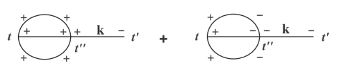
Figure 4.1: The Feynman diagrams that contribute to the quantum kinetic equation for a self-interacting scalar theory up to two-loop order.

At order $\lambda$, the right-hand side of Eq. (4.15) vanishes identically. This is a consequence of the fact that both the free quasiparticle Hamiltonian $H_{0}$ and the initial density matrix $\rho$ are diagonal in the basis of free quasiparticles number operator. Hence, the relaxation of quasiparticle distribution functions is solely due to the interaction between quasiparticles.

To order $\lambda^{2}$, we find that the final form of the kinetic equation is given by

$$\frac{d}{dt}n_{\mathbf{k}}(t)=-\frac{\lambda}{6\omega_{\mathbf{k}}}\,\lim_{t^{\prime}\to t}\frac{\partial}{\partial t^{\prime}}\left\langle[\phi^{3}(\mathbf{k},t)]^{+}\,\phi^{-}(-\mathbf{k},t^{\prime})\right\rangle,$$ (4.17)

with the understanding that no tadpole diagrams being included as they are automatically canceled by the terms containing $\Delta$ and the last term in Eq. (4.15). To two-loop order, the Feynman diagrams that contribute to Eq. (4.17) is displayed in Figure 4.1 and the resultant time evolution of the quasiparticle distribution function is given by

$$\frac{d}{dt}n_{\mathbf{k}}(t) = \frac{\lambda^{2}}{6\omega_{\mathbf{k}}}\int\prod_{i=1}^{3}\frac{d^{3}q_{i}}{(2\pi)^{3}2\omega_{\mathbf{q}_{i}}}\int^{t}_{t_{0}}dt^{\prime\prime}\,(2\pi)^{3}\delta^{3}(\mathbf{k}-\mathbf{q}_{1}-\mathbf{q}_{2}-\mathbf{q}_{3})$$ (4.18)

$$\times\Big{[}\mathcal{N}_{1}(t_{0})\cos[\Delta\omega_{1}(t-t^{\prime\prime})]+3\mathcal{N}_{2}(t_{0})\cos[\Delta\omega_{2}(t-t^{\prime\prime})]$$

$$+\,3\mathcal{N}_{3}(t_{0})\cos[\Delta\omega_{3}(t-t^{\prime\prime})]+\mathcal{N}_{4}(t_{0})\cos[\Delta\omega_{4}(t-t^{\prime\prime})]\Big{]},$$

where

$$\Delta\omega_{1}=\omega_{\mathbf{k}}+\omega_{\mathbf{q}_{1}}+\omega_{\mathbf{q}_{2}}+\omega_{\mathbf{q}_{3}},\quad\Delta\omega_{2}=\omega_{\mathbf{k}}+\omega_{\mathbf{q}_{1}}+\omega_{\mathbf{q}_{2}}-\omega_{\mathbf{q}_{3}},$$

$$\Delta\omega_{3}=\omega_{\mathbf{k}}-\omega_{\mathbf{q}_{1}}-\omega_{\mathbf{q}_{2}}+\omega_{\mathbf{q}_{3}},\quad\Delta\omega_{4}=\omega_{\mathbf{k}}-\omega_{\mathbf{q}_{1}}-\omega_{\mathbf{q}_{2}}-\omega_{\mathbf{q}_{3}},$$ (4.19)

and

$$\mathcal{N}_{1}(t) = [1+n_{\mathbf{k}}(t)][1+n_{\mathbf{q}_{1}}(t)][1+n_{\mathbf{q}_{2}}(t)][1+n_{\mathbf{q}_{3}}(t)]-n_{\mathbf{k}}(t)\,n_{\mathbf{q}_{1}}(t)\,n_{\mathbf{q}_{2}}(t)\,n_{\mathbf{q}_{3}}(t),$$

$$\mathcal{N}_{2}(t) = [1+n_{\mathbf{k}}(t)][1+n_{\mathbf{q}_{1}}(t)][1+n_{\mathbf{q}_{2}}(t)]\,n_{\mathbf{q}_{3}}(t)-n_{\mathbf{k}}(t)\,n_{\mathbf{q}_{1}}(t)\,n_{\mathbf{q}_{2}}(t)\,[1+n_{\mathbf{q}_{3}}(t)],$$

$$\mathcal{N}_{3}(t) = [1+n_{\mathbf{k}}(t)]\,n_{\mathbf{q}_{1}}(t)\,n_{\mathbf{q}_{2}}(t)\,[1+n_{\mathbf{q}_{3}}(t)]-n_{\mathbf{k}}(t)\,[1+n_{\mathbf{q}_{1}}(t)][1+n_{\mathbf{q}_{2}}(t)]\,n_{\mathbf{q}_{3}}(t),$$

$$\mathcal{N}_{4}(t) = [1+n_{\mathbf{k}}(t)]\,n_{\mathbf{q}_{1}}(t)\,n_{\mathbf{q}_{2}}(t)\,n_{\mathbf{q}_{3}}(t)-n_{\mathbf{k}}(t)\,[1+n_{\mathbf{q}_{1}}(t)][1+n_{\mathbf{q}_{2}}(t)][1+n_{\mathbf{q}_{3}}(t)].$$

The kinetic equation (4.18) is retarded and causal. The different contributions have a physical interpretation in terms of the ‘gain minus loss’ processes in the plasma. The first term describes the creation of four particles minus the destruction of four particles in the plasma, the second and fourth terms describe the creation of three particles and destruction of one minus destruction of three and creation of one, the third term is the scattering of two particles off two particles and is the usual Boltzmann term.

As will be discussed in detail below, such a perturbative expansion will be meaningful for times $t\ll t_{\mathrm{kin}}$, where $t_{\mathrm{kin}}$ is the kinetic time scale for the nonequilibrium distribution functions. For small enough coupling we expect that $t_{\mathrm{kin}}$ will be large enough such that there is a wide separation between the microscopic and the kinetic time scales that will warrant such an approximation (see below).

Since the propagators entering in the perturbative expansion of the evolution equation are in terms of the quasiparticle distribution functions at the initial time $t_{0}$, the time integration in Eq. (LABEL:scalar:ocupanumber) can be done straightforwardly leading to the following equation:

$$\frac{d}{dt}n_{\mathbf{k}}(t)=\frac{\lambda^{2}}{3}\int_{-\infty}^{+\infty}d\omega\,\mathcal{R}[\omega,\mathbf{k};\mathcal{N}_{j}(t_{0})]\,\frac{\sin[(\omega-\omega_{\mathbf{k}})(t-t_{0})]}{\pi(\omega-\omega_{\mathbf{k}})},$$ (4.21)

where

$$\mathcal{R}[\omega,\mathbf{k};\mathcal{N}_{j}(t_{0})] = \frac{\pi}{2\omega_{\mathbf{k}}}\,\int\prod_{i=1}^{3}\frac{d^{3}q_{i}}{(2\pi)^{3}2\omega_{\mathbf{q}_{i}}}\,(2\pi)^{3}\delta^{3}(\mathbf{k}-\mathbf{q}_{1}-\mathbf{q}_{2}-\mathbf{q}_{3})\Big{[}\mathcal{N}_{1}(t_{0})\,\delta(\Delta\omega_{1})$$ (4.22)

$$+\,3\,\mathcal{N}_{2}(t_{0})\,\delta(\Delta\omega_{2})+3\,\mathcal{N}_{3}(t_{0})\,\delta(\Delta\omega_{3})+\mathcal{N}_{4}(t_{0})\,\delta(\Delta\omega_{4})\Big{]},$$

with $j=1,\ldots,4$.

We are now ready to solve the kinetic equation derived above. Since $\mathcal{R}[\omega,\mathbf{k};\mathcal{N}_{j}(t_{0})]$ is fixed at initial time $t_{0}$, Eq. (4.21) can be solved by direct integration over $t$, thus leading to

$$n_{\mathbf{k}}(t)=n_{\mathbf{k}}(t_{0})+\frac{\lambda^{2}}{3}\int_{-\infty}^{+\infty}d\omega\,\mathcal{R}[\omega,\mathbf{k};\mathcal{N}_{j}(t_{0})]\frac{1-\cos[(\omega-\omega_{\mathbf{k}})(t-t_{0})]}{\pi(\omega-\omega_{\mathbf{k}})^{2}}.$$ (4.23)

It is noted that the above expression gives the time evolution of the quasiparticle distribution function to lowest order in perturbation theory, but only for early times. To make this statement more precise, let us consider the following approximation

$$\lim_{t-t_{0}\to\infty}\frac{1-\cos[(\omega-\omega_{\mathbf{k}})(t-t_{0})]}{\pi(\omega-\omega_{\mathbf{k}})^{2}}=(t-t_{0})\,\delta(\omega-\omega_{\mathbf{k}}).$$ (4.24)

Thus, provided that $\mathcal{R}[\omega,\mathbf{k};\mathcal{N}_{j}(t_{0})]$ is finite at $\omega=\omega_{\mathbf{k}}$, one finds that $n_{\mathbf{k}}(t)$ at large times is given by

$$n_{\mathbf{k}}(t) = n_{\mathbf{k}}(t_{0})+\frac{\lambda^{2}}{3}\,\mathcal{R}[\omega_{\mathbf{k}},\mathbf{k};\mathcal{N}_{j}(t_{0})]\,(t-t_{0})+\mbox{nonsecular terms},$$ (4.25)

where the nonsecular terms denotes terms that are bound at all times. In the above expression, the term that grows (linearly) with time is referred to as a secular term. The approximation above, replacing the oscillatory terms with resonant denominators by $t\,\delta(\omega-\omega_{\mathbf{k}})$ is the same as that invoked in ordinary time-dependent perturbation theory leading to Fermi’s golden rule in elementary time-dependent perturbation theory .

Clearly, the presence of secular terms in time restricts the validity of the perturbative expansion to a time interval $t-t_{0}\ll t_{\mathrm{kin}}$ with

$$t_{\mathrm{kin}}(k)\approx\frac{3\,n_{\mathbf{k}}(t_{0})}{\lambda^{2}\,\mathcal{R}[\omega_{\mathbf{k}},\mathbf{k};\mathcal{N}_{j}(t_{0})]}.$$ (4.26)

Since the time scales in the integral in Eq. (4.23) are of the order of or shorter than $t_{\mathrm{mic}}\sim 1/m_{\mathrm{eff}}$ the asymptotic form given by Eq. (4.25) is valid for $t-t_{0}\gg t_{\mathrm{mic}}$. Therefore for weak coupling there is a regime of intermediate asymptotics in time defined by

$$t_{\mathrm{mic}}\ll t-t_{0}\ll t_{\mathrm{kin}}(k),$$ (4.27)

such that perturbation theory is valid and the corrections to the quasiparticle distribution function is dominated by the secular term.

We note two important features of this analysis:

(i) In the intermediate asymptotic regime (4.27) the only explicit dependence on the initial time $t_{0}$ is in the secular term, since $\mathcal{R}[\omega_{\mathbf{k}},\mathbf{k};\mathcal{N}_{j}(t_{0})]$ depends on $t_{0}$ only implicitly through the initial distribution functions. These observations will become important for the analysis that follows below.

(ii) The function(al) $\mathcal{R}[\omega_{\mathbf{k}},\mathbf{k};\mathcal{N}_{j}(t_{0})]$ given by Eq. (4.22) vanishes if the initial distribution functions are the equilibrium ones as a result of the energy conservation delta functions and the equilibrium relation $1+n_{B}(\omega)=e^{\beta\omega}n_{B}(\omega)$. In this case there are no secular terms in the perturbative expansion.

To highlight the significance of the second point above in a manner that will allow us to establish contact with the issue of pinch singularities in a later section, we note that the secular term in Eq. (4.25) corresponds to the net change of quasiparticles distribution function in the time interval $t-t_{0}$. To see this more explicitly, we note that $\mathcal{R}[\omega_{\mathbf{k}},\mathbf{k};\mathcal{N}_{j}(t_{0})]$ can be rewritten as

$$\frac{\lambda^{2}}{3}\mathcal{R}[\omega_{\mathbf{k}},\mathbf{k};\mathcal{N}_{j}(t_{0})]=\frac{i}{2\omega_{\mathbf{k}}}\Big{[}[1+n_{\mathbf{k}}(t_{0})]\,\Sigma^{<}(\omega_{\mathbf{k}},\mathbf{k})-n_{\mathbf{k}}(t_{0})\,\Sigma^{>}(\omega_{\mathbf{k}},\mathbf{k})\Big{]},$$ (4.28)

where $\Sigma^{>}(\omega_{\mathbf{k}},\mathbf{k})-\Sigma^{<}(\omega_{\mathbf{k}},\mathbf{k})=2\,i\,\mathrm{Im}\Sigma_{R}(\omega_{\mathbf{k}},\mathbf{k})$ with $\Sigma_{R}(\omega_{\mathbf{k}},\mathbf{k})$ the on-shell retarded self-energy calculated to two-loop order in terms of the initial distribution functions $n_{\mathbf{k}}(t_{0})$ [71] . Thus, the absence of secular term for a system in thermal equilibrium [for which $n_{\mathbf{k}}(t_{0})=n_{B}(\omega_{\mathbf{k}})$] is a consequence of the Kubo-Martin-Schwinger (KMS) condition for the equilibrium self-energy

$$\Sigma^{>}(\omega,\mathbf{k})=e^{\beta\omega}\Sigma^{<}(\omega,\mathbf{k}).$$ (4.29)

Furthermore, it can be recognized that the first (second) term in Eq. (4.28), corresponds to the “gain” (“loss”) part in the usual Boltzmann type collision term. Hence, one can readily interpret $\lambda^{2}\mathcal{R}[\omega_{\mathbf{k}},\mathbf{k};\mathcal{N}_{j}(t_{0})]/3$ as the net production rate of quasiparticles per unit time.

4.2.2 Dynamical renormalization group equation

Secular divergences are an ubiquitous feature in the perturbative solution of differential equations with oscillatory behavior. A resummation method based on the idea of the renormalization group (RG) that improves the perturbative solutions of differential equations was introduced by Goldenfeld and collaborators [93] to study pattern formation in condensed matter systems. As explained in details in Refs. [93, 94], this powerful method not only allows a consistent resummation of the secular terms in the perturbative expansion but also provides a consistent reduction of the dynamics to the slow degrees of freedom. In a recent development, this method has been generalized to the realm of nonequilibrium quantum field theory as a dynamical renormalization group to resum the perturbative series for the real time evolution of nonequilibrium expectation values [84, 95]. This generalization is a major step since in nonequilibrium systems the equations of motion for expectation values are nonlocal and, as will be shown below, require a resummation of Feynman diagrams.

Having recognized that a time scale emerges in the perturbative expansion (4.25) due to the presence of the secular term, we now implement the dynamical renormalization group resummation of secular divergences to improve the perturbative expansion following the formulation presented in Ref. [84].

To lowest order, this resummation is achieved by introducing the “renormalized” initial distribution functions $n_{\mathbf{k}}(\tau)$ which are related to the “bare” initial distribution function $n_{\mathbf{k}}(t_{0})$ via a renormalization constant $\mathcal{Z}_{\mathbf{k}}(\tau,t_{0})$ given by

$$n_{\mathbf{k}}(t_{0})=\mathcal{Z}_{\mathbf{k}}(\tau,t_{0})\,n_{\mathbf{k}}(\tau),\qquad\mathcal{Z}_{\mathbf{k}}(\tau,t_{0})=1+\frac{\lambda^{2}}{3}\,z_{\mathbf{k}}(\tau,t_{0})+\mathcal{O}(\lambda^{4}),$$ (4.30)

where $\tau$ is an arbitrary “renormalization scale” and $z_{\mathbf{k}}(\tau,t_{0})$ will be chosen to cancel the secular term on a time scale $\tau$. Substitute Eq. (4.30) into Eq. (4.25), to order $\lambda^{2}$ we obtain

$$n_{\mathbf{k}}(t)=n_{\mathbf{k}}(\tau)+\frac{\lambda^{2}}{3}\,\left[z_{\mathbf{k}}(\tau,t_{0})n_{\mathbf{k}}(\tau)+(t-t_{0})\,\mathcal{R}[\omega_{\mathbf{k}},\mathbf{k};\mathcal{N}_{j}(\tau)]\,\right]+\mathcal{O}(\lambda^{4}).$$ (4.31)

Thus, to this order, the choice

$$z_{\mathbf{k}}(\tau,t_{0})=-(\tau-t_{0})\frac{\mathcal{R}[\omega_{\mathbf{k}},\mathbf{k};\mathcal{N}_{j}(\tau)]}{n_{\mathbf{k}}(\tau)}$$ (4.32)

leads to

$$n_{\mathbf{k}}(t)=n_{\mathbf{k}}(\tau)+\frac{\lambda^{2}}{3}\,(t-\tau)\,\mathcal{R}[\omega_{\mathbf{k}},\mathbf{k};\mathcal{N}_{j}(\tau)]+\mathcal{O}(\lambda^{4}).$$ (4.33)

Whereas the original perturbative solution was only valid for times such that the contribution from the secular term remains very small compared to the initial distribution function at time $t_{0}$, the renormalized solution Eq. (4.33) is valid for time intervals $t-\tau$ such that the secular term remains small, thus by choosing $\tau$ arbitrarily close to $t$ we have improved the perturbative expansion [93, 94].

To find the dependence of $n_{\mathbf{k}}(\tau)$ on $\tau$, we make use of the fact that the “physical” distribution function $n_{\mathbf{k}}(t)$ does not depend on the arbitrary scale $\tau$ as a change in the renormalization point $\tau$ is compensated by a change in the “renormalized” initial distribution functions $n_{\mathbf{k}}(\tau)$. This $\tau$-independence leads to the dynamical renormalization group equation, which to lowest order is given by

$$\frac{d}{d\tau}n_{\mathbf{k}}(\tau)-\frac{\lambda^{2}}{3}\,\mathcal{R}[\omega_{\mathbf{k}},\mathbf{k};\mathcal{N}_{j}(\tau)]=0.$$ (4.34)

This renormalization of the distribution function also affects the effective mass of the quasiparticles since $m^{2}_{\mathrm{eff}}$ is determined from the self-consistent equation (4.5), which is a consequence of the tadpole cancelation consistently in perturbation theory. Since the effective mass is a functional of the distribution function it will be renormalized consistently. This is physically correct since the in-medium effective masses will change under the time evolution of the distribution functions. Choosing the arbitrary scale $\tau$ to coincide with the time $t$ in Eq. (4.34), we obtain the resummed quantum kinetic equation:

$$\frac{d}{dt}n_{\mathbf{k}}(t) = \frac{\pi\lambda^{2}}{6\omega_{\mathbf{k}}}\int\frac{d^{3}q_{1}}{(2\pi)^{3}2\omega_{\mathbf{q}_{1}}}\frac{d^{3}q_{2}}{(2\pi)^{3}2\omega_{\mathbf{q}_{2}}}\frac{d^{3}q_{3}}{(2\pi)^{3}2\omega_{\mathbf{q}_{3}}}(2\pi)^{3}\delta^{3}(\mathbf{k}-\mathbf{q}_{1}-\mathbf{q}_{2}-\mathbf{q}_{3})$$

$$\times\Big{[}\delta(\omega_{\mathbf{k}}+\omega_{\mathbf{q}_{1}}+\omega_{\mathbf{q}_{2}}+\omega_{\mathbf{q}_{3}})\,\mathcal{N}_{1}(t)+3\,\delta(\omega_{\mathbf{k}}+\omega_{\mathbf{q}_{1}}+\omega_{\mathbf{q}_{2}}-\omega_{\mathbf{q}_{3}})\,\mathcal{N}_{2}(t)$$

$$+\,3\,\delta(\omega_{\mathbf{k}}-\omega_{\mathbf{q}_{1}}-\omega_{\mathbf{q}_{2}}+\omega_{\mathbf{q}_{3}})\,\mathcal{N}_{3}(t)+\delta(\omega_{\mathbf{k}}-\omega_{\mathbf{q}_{1}}-\omega_{\mathbf{q}_{2}}-\omega_{\mathbf{q}_{3}})\,\mathcal{N}_{4}(t)\Big{]},$$

where the $\mathcal{N}_{j}(t)$ are given in Eq. (LABEL:scalar:ocupanumber).

To avoid cluttering of notation in the above expression, we have not made explicit the fact that the frequencies $\omega_{\mathbf{q}}=\sqrt{\mathbf{q}^{2}+m_{\mathrm{eff}}^{2}}$ depend on time through the time dependence of $m_{\mathrm{eff}}$, which is in turn determined by the time dependence of the quasiparticle distribution function. Indeed, the dynamical renormalization group resummation leads at once to the conclusion that the cancelation of tadpole terms by a proper choice of $\Delta$ requires that at every time $t$ the effective mass is the solution of the time-dependent gap equation

$$m^{2}_{\mathrm{eff}}(t)=m^{2}+\frac{\lambda}{2}\int\frac{d^{3}q}{(2\pi)^{3}}\frac{n_{\mathbf{q}}(t)}{\sqrt{q^{2}+m^{2}_{\mathrm{eff}}(t)}},$$ (4.36)

where $n_{\mathbf{q}}(t)$ is the solution of the kinetic equation (LABEL:resucinetica). Thus, the full quantum kinetic equation that includes a nonequilibrium generalization of the hard thermal loop resummation in this scalar theory is given by Eq. (LABEL:resucinetica) with the replacement $\omega_{\mathbf{q}}\rightarrow\omega_{\mathbf{q}}(t)$, where $\omega_{\mathbf{q}}(t)$ are the solutions of the self-consistent time-dependent gap equation (4.36).

The quantum kinetic equation (LABEL:resucinetica) is therefore more general than the familiar semiclassical Boltzmann equation for a scalar field theory in that it includes the proper in-medium modifications of the quasiparticle masses. This approach provides an alternative derivation of the self-consistent method proposed in Ref. [70].

It is now evident that the dynamical renormalization group systematically resums the secular terms and the corresponding dynamical renormalization group equation extracts the slow evolution of the nonequilibrium system.

For small departures from equilibrium the time scales for relaxation can be obtained by linearizing the kinetic equation (LABEL:resucinetica) around the equilibrium solution at $t=t_{0}$. This is the relaxation time approximation which assumes that the quasiparticle distribution function for a fixed mode of momentum $\mathbf{k}$ is perturbed slightly off equilibrium such that $n_{\mathbf{k}}(t_{0})=n_{B}(\omega_{\mathbf{k}})+\delta n_{\mathbf{k}}(t_{0})$, while all the other modes remain in equilibrium.

Recognizing that only the delta function $\delta(\omega_{\mathbf{k}}-\omega_{\mathbf{q}_{1}}-\omega_{\mathbf{q}_{2}}+\omega_{\mathbf{q}_{3}})$ that multiplies the scattering term $\mathcal{N}_{3}(t)$ in Eq. (LABEL:resucinetica) is fulfilled, one finds that the linearized kinetic equation reads

$$\frac{d}{dt}\delta n_{\mathbf{k}}(t)=-\Gamma(k)\,\delta n_{\mathbf{k}}(t),$$ (4.37)

where $\Gamma(k)$ is the scalar interaction rate

$$\Gamma(k) = \frac{\lambda^{2}\pi}{2\omega_{\mathbf{k}}}\int\frac{d^{3}q_{1}}{(2\pi)^{3}2\omega_{\mathbf{q}_{1}}}\frac{d^{3}q_{2}}{(2\pi)^{3}2\omega_{\mathbf{q}_{2}}}\frac{d^{3}q_{3}}{(2\pi)^{3}2\omega_{\mathbf{q}_{3}}}(2\pi)^{3}\delta^{3}(\mathbf{k}-\mathbf{q}_{1}-\mathbf{q}_{2}-\mathbf{q}_{3})$$ (4.38)

$$\times\,\delta(\omega_{\mathbf{k}}-\omega_{\mathbf{q}_{1}}-\omega_{\mathbf{q}_{2}}+\omega_{\mathbf{q}_{3}})\Big{[}[1+n_{B}(\omega_{\mathbf{q}_{1}})]\,[1+n_{B}(\omega_{\mathbf{q}_{2}})]\,n_{B}(\omega_{\mathbf{q}_{3}})$$

$$-\,n_{B}(\omega_{\mathbf{q}_{1}})\,n_{B}(\omega_{\mathbf{q}_{2}})\,[1+n_{B}(\omega_{\mathbf{q}_{3}})]\Big{]},$$

where $\omega_{\mathbf{k}}=\sqrt{\mathbf{k}^{2}+m_{\mathrm{eff}}^{2}(T)}$. Solving Eq. (4.37) with the initial distribution $\delta n_{\mathbf{k}}(t_{0})$, one finds that the quasiparticle distribution function in the relaxation time approximation evolves in time in the following manner

$$\delta n_{\mathbf{k}}(t)=\delta n_{\mathbf{k}}(t_{0})\,e^{-\Gamma(k)(t-t_{0})},$$ (4.39)

which gives the time scales for relaxation close to thermal equilibrium.

In the case of soft momentum ($k\ll m_{\mathrm{eff}}(T)\ll T$) and high temperature ($\lambda T^{2}\gg m^{2}$), one obtains [71]

$$t_{\mathrm{kin}}(k\approx 0)\equiv\frac{1}{\Gamma({k\approx 0})}\approx\frac{32\sqrt{24\pi}}{\lambda^{3/2}~{}T}.$$ (4.40)

For very weak coupling (as we have assumed), the kinetic time scale is much larger that the microscopic one $t_{\mathrm{mic}}\sim 1/m_{\mathrm{eff}}\sim 1/\sqrt{\lambda}\,T$, since $t_{\mathrm{kin}}/t_{\mathrm{mic}}\sim 1/\lambda\gg 1$. This verifies the assumption of the separation of microscopic and kinetic time scales in the weak coupling limit.

4.3 Comparison to the Euclidean Renormalization Group

In the section we establish a very close relationship between the dynamical renormalization group discussed above and the usual renormalization group in Euclidean field theory by demonstrating that the rationale behind the two methods are identical and that there exists an one-to-one correspondence between them.

First we review the idea of the Euclidean renormalization group in zero-temperature field theory. Let us consider a (massless) scalar field theory in four dimensions with an upper momentum cutoff $\Lambda$ described by the Lagrangian density

$${\cal{L}}[\phi]=\frac{1}{2}\left(\partial_{\mu}\phi\right)^{2}-\frac{\lambda_{0}}{4!}\phi^{4},$$ (4.41)

where $\lambda_{0}$ is the bare coupling. As an example, we calculate the two particles to two particles scattering amplitude in perturbation theory. The one-particle-irreducible (1PI) four-point function (i.e., two particles to two particles scattering amplitude) at an off-shell symmetric point to one-loop order in Euclidean space is given by

$$\Gamma^{(4)}(p,p,p,p)=\lambda_{0}-\frac{3}{2}\lambda_{0}^{2}\,\ln\frac{\Lambda}{p}+\mathcal{O}(\lambda_{0}^{3}),$$ (4.42)

where $p$ is the Euclidean four-momentum. Clearly perturbation theory breaks down for $\Lambda/p\gtrsim e^{1/\lambda_{0}^{2}}$.

Let us introduce the renormalized coupling constant at a momentum scale $\kappa$ as usual as

$$\lambda_{0}=\mathcal{Z}_{\lambda}(\kappa)\,\lambda(\kappa),\quad\mathcal{Z}_{\lambda}(\kappa)=1+z_{1}(\kappa)\,\lambda(\kappa)+\mathcal{O}(\lambda^{3}),$$ (4.43)

and choose $z_{1}(\kappa)$ to cancel the logarithmic divergence at an arbitrary renormalization scale $\kappa$. Then in terms of $\lambda(\kappa)$ the scattering amplitude $\Gamma^{(4)}(p,p,p,p)$ becomes

$$\Gamma^{(4)}(p,p,p,p)=\lambda(\kappa)+\frac{3}{2}\lambda^{2}(\kappa)\,\ln\frac{p}{\kappa}+\mathcal{O}(\lambda^{3}),$$ (4.44)

with $\Gamma^{(4)}(\kappa,\kappa,\kappa,\kappa)=\lambda(\kappa)$. The scattering amplitude does not depend on the arbitrary renormalization scale $\kappa$ and this independence implies $\kappa\,\partial\Gamma^{(4)}(p,p,p,p)/\partial\kappa=0$, which in turn to lowest order leads to the renormalization group equation

$$\kappa\,\frac{d\lambda(\kappa)}{d\kappa}=\beta(\lambda),\qquad\beta(\lambda)=\frac{3}{2}\lambda^{2}(\kappa)+\mathcal{O}(\lambda^{3}),$$ (4.45)

where $\beta(\lambda)$ is referred to as the renormalization group beta function. Solving this renormalization group equation with an initial condition $\lambda(\bar{p})=\bar{\lambda}$ that determines the scattering amplitude at some value of the momentum and choosing $\kappa=p$ in Eq. (4.44), one obtains the renormalization group improved scattering amplitude (at an off-shell symmetric point)

$$\Gamma^{(4)}(p,p,p,p;\bar{\lambda}(\bar{p}))=\lambda(p),$$ (4.46)

with $\lambda(p)$ the solution of the renormalization group equation

$$\lambda(p)=\frac{\bar{\lambda}}{\raisebox{-2.15277pt}{$1-(3\bar{\lambda}/2)\ln(p/\bar{p})$}}.$$ (4.47)

The connection between the renormalization group in momentum space and the dynamical renormalization group in real time (resummation of secular terms) used in the previous section is immediate through the identification

$$t_{0}\Leftrightarrow\ln(\Lambda/\bar{p}),\qquad t\Leftrightarrow\ln(p/\bar{p}),\qquad\tau\Leftrightarrow\ln(\kappa/\bar{p}),$$

which when replaced into Eq. (4.42) illuminates the formal equivalence with secular terms.

This simple analysis highlights how the dynamical renormalization group does precisely the same in the real time as the renormalization group in zero-temperature Euclidean field theory. Much in the same manner that the renormalization group improved scattering amplitude given by Eq. (4.46) is a resummation of the perturbative expansion, the kinetic equation obtained from the dynamical renormalization group improvement represents a resummation of the perturbative expansion in real time. The lowest order renormalization group equation (4.45) resums the leading logarithms, while the lowest order dynamical renormalization group equation resums the leading secular terms.

Dynamical renormalization group: fixed points and coarse-graining

The similarity between the renormalization of distribution functions and the renormalization of couplings suggests that the collision terms of the quantum kinetic equation can be interpreted as beta functions of the dynamical renormalization group and that the space of distribution functions can be interpreted as the space of coupling constants. The dynamical renormalization group trajectories determine the flow in this space, therefore fixed points of the dynamical renormalization group describe stationary solutions with given distribution functions. Thermal equilibrium distributions are thus fixed points of the dynamical renormalization group. Furthermore, there can be other stationary solutions with non-thermal distribution functions, e.g., those describing turbulent behavior [96]. Linearizing the renormalization group equation around the fixed points corresponds to linearizing the kinetic equation near equilibrium and the linear eigenvalues are related to the relaxation rates in the relaxation time approximation.

One can establish a closer relationship to the usual renormalization program of field theory in its momentum shell version with the following alternative interpretation of the secular terms and their resummation.

The initial distribution at a time $t_{0}$ is evolved in time perturbatively up to a time $t_{0}+\Delta t$ such that the perturbative expansion is still valid, i.e., $t_{\mathrm{kin}}\gg\Delta t$ with $t_{\mathrm{kin}}$ the kinetic time scale. Secular terms begin to dominate the perturbative expansion on a time scale $\Delta t\gg t_{\mathrm{mic}}$ with $t_{\mathrm{mic}}$ the microscopic time scale. Thus if there is a separation of time scales such that $t_{\mathrm{kin}}\gg\Delta t\gg t_{\mathrm{mic}}$, then in this intermediate asymptotic regime perturbation theory is reliable but secular terms appear and can be isolated.

A renormalization of the distribution function absorbs the contribution from the secular terms. The “renormalized” distribution function is used as an initial condition at $t_{0}+\Delta t$ to iterate forward in time to $t_{0}+2\Delta t$ using the perturbative expansion, but with the propagators in terms of the distribution function at the time $t_{0}+\Delta t$. This procedure can be carried out “infinitesimally” (in the sense compared with the kinetic time scale) and the differential equation that describes the changes of the distribution function under the intermediate asymptotic time evolution is the dynamical renormalization group equation.

This has an obvious similarity to the renormalization group in terms of integrating in momentum shells. The result of integrating out degrees of freedom in a momentum shell are absorbed into a renormalization of the couplings and an effective theory at a lower scale but in terms of the effective couplings. This procedure is carried out infinitesimally and the differential equation that describes the changes of the couplings under integrating out degrees of freedom in these momentum shells is the renormalization group equation.

An important aspect of this procedure of evolving in time and “resetting” the distribution functions is that in this process it is implicitly assumed that the density matrix at later times remains diagonal in the basis of free quasiparticle number operators. Clearly, if at the initial time the density matrix was diagonal in this basis, because the interaction Hamiltonian does not commute with the density matrix, off-diagonal density matrix elements will be generated upon time evolution. In resetting the distribution functions and using the propagators in terms of these updated distribution functions we have neglected off-diagonal correlations, e.g., correlations of the form $\langle a(\mathbf{k},t)a(\mathbf{k},t)\rangle$ and its complex conjugate will be generated upon time evolution. In neglecting these off-diagonal terms we are introducing coarse-graining. Indeed, two stages of coarse-graining had been introduced: (i) integrating in time up to an intermediate asymptotics and resumming the secular terms neglect transient phenomena, i.e., averages over the microscopic time scales, and (ii) off-diagonal matrix elements (in the basis of free quasiparticle number operators) had been neglected. The coarse graining also has an counterpart in the language of the renormalization group in Euclidean field theory, i.e., neglecting the irrelevant couplings that are generated upon integrating out shorter scales. Keeping all of the correlations in the density matrix would be equivalent to Wilson’s approach to renormalization group, in which all possible couplings are included in the Lagrangian and all of them are maintained in the renormalization on the same footing.

4.4 Application: $\boldsymbol{O(4)}$ Linear Sigma Model

In this section we apply the dynamical renormalization group method to derive kinetic equations for pions and sigma mesons in the $O(4)$ linear sigma model, which is an effective theory of low energy QCD describing the hadronic world. We recall that the sigma condensate $\langle\sigma\rangle$ represents the quark condensate $\langle\bar{q}q\rangle$ in the sense that they both have the same transformation properties, corresponding to two flavors of massless quarks. At high temperatures, quarks and gluons exist in a deconfined, chirally symmetric phase. At some critical temperature of order 160 MeV a transition to a hadronic phase occurs. In this confined and chiral symmetry broken phase the quark condensate is nonzero.

The Lagrangian density of the $O(4)$ linear sigma model in the limit of exact chiral symmetry, i.e., without an explicit symmetry-breaking term, is given by

$${\cal L}[{\boldsymbol{\pi}},\sigma]=\frac{1}{2}\left(\partial_{\mu}{\boldsymbol{\pi}}\right)^{2}+\frac{1}{2}\left(\partial_{\mu}\sigma\right)^{2}-\frac{\lambda}{4}\left({\boldsymbol{\pi}}^{2}+\sigma^{2}-f_{\pi}^{2}\right)^{2},$$ (4.48)

where $\boldsymbol{\pi}=(\pi^{1},\pi^{2},\pi^{3})$ and $f_{\pi}\sim 93$ MeV is the pion decay constant. At high temperature $T>T_{c}$, where $T_{c}\sim f_{\pi}$ is the critical temperature, the $O(4)$ symmetry is restored by a second order phase transition [97].

In the symmetric phase pions and sigma mesons are degenerate, and the linear sigma model reduces to a self-interacting scalar theory, analogous to that discussed in Sec. 4.2. Thus, we limit our discussion here to the low temperature broken symmetry phase in which the temperature $T\ll f_{\pi}$. Since at low temperature the $O(4)$ symmetry is spontaneously broken via the sigma condensate $\langle\sigma\rangle$, we shift the sigma field $\sigma(\mathbf{x},t)=\bar{\sigma}(\mathbf{x},t)+v$, where $v$ is temperature dependent and yet to be determined.

In thermal equilibrium $v$ is fixed by requiring that $\left\langle\bar{\sigma}(\mathbf{x},t)\right\rangle=0$ to all orders in perturbation theory for temperature $T<T_{c}$. In nonequilibrium this split must be performed on both forward $(+)$ and backward $(-)$ time branches, writing the sigma field $\sigma^{\pm}(\mathbf{x},t)$ as

$$\sigma^{\pm}(\mathbf{x},t)=\bar{\sigma}^{\pm}(\mathbf{x},t)+v,\qquad\langle\bar{\sigma}^{\pm}(\mathbf{x},t)\rangle=0,$$ (4.49)

where $\langle\,\cdot\,\rangle$ denotes the nonequilibrium expectation value. The expectation value $v$ is determined by requiring that the expectation value of $\bar{\sigma}(\mathbf{x},t)$ vanishes to all orders in perturbation theory via the tadpole method [45]. One finds to one-loop order the equation that determines $v$ is given by

$$v\left[v^{2}-f_{\pi}^{2}+\langle{\boldsymbol{\pi}}^{2}\rangle+3\langle\bar{\sigma}^{2}\rangle\right]=0.$$ (4.50)

We emphasize that in perturbation theory $v$ depends on the initial nonequilibrium distribution functions of the pions and sigma mesons, which in turn implies that after dynamical renormalization group resummation $v$ acquires implicit time dependence through the time dependence of the distribution functions (see Sec. 3.2). Once the solution of this equation for $v$ is used in the perturbative expansion to one loop order, the tadpole diagrams that arise from the shift in the field cancel automatically to this order. This feature of cancelation of tadpole diagrams that would result in an expectation value of $\bar{\sigma}$ by the consistent use of the tadpole equation persists to all orders in perturbation theory.

A solution of Eq. (4.50) with $v\neq 0$ signals broken symmetry and massless pions (in the strict chiral limit). Therefore once the correct expectation value $v$ is used, the one-particle-reducible (1PR) tadpole diagrams do not contribute in the perturbative expansion of the kinetic equation. To this order the inverse pion propagator for zero energy and momentum reads

$$G^{-1}_{\pi}(\omega=0,\mathbf{k}=\mathbf{0})=-\lambda\left[v^{2}-f_{\pi}^{2}+\langle{\boldsymbol{\pi}}^{2}\rangle+3\langle\bar{\sigma}^{2}\rangle\right],$$ (4.51)

which vanishes whenever $v\neq 0$ by the tadpole condition Eq. (4.50), hence the Goldstone theorem is satisfied and the pions are the Goldstone bosons.

The study of the relaxation of sigma mesons (resonance) and pions near and below the chiral phase transition is an important phenomenological aspect of low energy chiral phenomenology with relevance to heavy ion collisions. Furthermore, recent studies have revealed interesting features associated with the dropping of the sigma mass near the chiral transition and the enhancement of threshold effects with potential experimental consequences [89]. The kinetic approach described here could prove useful to further assess the contributions to the width of the sigma meson near the chiral phase transition, this is an important study on its own right and we expect to report on these issues in the near future.

With the purpose of comparing to recent results, we now focus on the situation at low temperatures under the assumption that the distribution functions of sigma mesons and pions are not too far from equilibrium, i.e., cool pions and sigma mesons. At low temperatures the relaxation of pions and sigma mesons will be dominated by the one-loop contributions, and the scattering contributions will be subleading. The scattering contributions are of the same form as those discussed for the scalar theory and involve at least two distribution functions and are subdominant in the low temperature limit as compared to the one-loop contributions described below.

Since the linear sigma model is renormalizable and we focus on the medium (finite-temperature) effects, we ignore the vacuum (zero-temperature) ultraviolet divergences which can be absorbed into a renormalization of $f_{\pi}$. For a small departure from thermal equilibrium, one can approximate $\langle{\boldsymbol{\pi}}^{2}\rangle$ and $\langle\bar{\sigma}^{2}\rangle$ by their thermal equilibrium values

$$\langle{\boldsymbol{\pi}}^{2}\rangle=\frac{T^{2}}{4},\qquad\langle\bar{\sigma}^{2}\rangle=\int\frac{d^{3}q}{(2\pi)^{3}\omega_{\mathbf{q}}}\,n_{B}(\omega_{\mathbf{q}}),$$ (4.52)

respectively, where $\omega_{\mathbf{q}}=\sqrt{\mathbf{q}^{2}+m_{\sigma}^{2}}$ with the sigma mass $m_{\sigma}^{2}=2\lambda v^{2}$ being determined self-consistently. In the low temperature limit $T\ll f_{\pi}$, one finds $v^{2}=f_{\pi}^{2}\,[1-\mathcal{O}(T^{2}/f_{\pi}^{2})]$ and $m_{\sigma}=\sqrt{2\lambda}\,f_{\pi}[1-\mathcal{O}(T^{2}/f_{\pi}^{2})]$. Thus in our discussion below where $T\ll f_{\pi}$, we set $v=f_{\pi}$ and $m_{\sigma}=\sqrt{2\lambda}f_{\pi}$. The main reason behind this analysis is to display the microscopic time scales for the mesons: $t^{\sigma}_{\mathrm{mic}}\leq 1/m_{\sigma}$ and $t^{\pi}_{\mathrm{mic}}=1/k$ with $k$ being the momentum of the pion. The validity of a kinetic description will hinge upon the kinetic time scales being much longer than these microscopic scales.

Upon the above replacement, one can rewrite the Lagrangian for the cool linear sigma model to lowest order as

$${\cal L}[{\boldsymbol{\pi}},\sigma]=\frac{1}{2}\left(\partial_{\mu}{\boldsymbol{\pi}}\right)^{2}+\frac{1}{2}\left(\partial_{\mu}\sigma\right)^{2}-\frac{1}{2}m_{\sigma}^{2}\sigma^{2}-\lambda f_{\pi}\left(\sigma{\boldsymbol{\pi}}^{2}+\sigma^{3}\right)-\frac{\lambda}{4}\left({\boldsymbol{\pi}}^{2}+\sigma^{2}\right)^{2},$$ (4.53)

where the bar over the shifted sigma field has been omitted for simplicity of notation.

Our goal in this section is to derive the kinetic equations describing pion and sigma meson relaxation to lowest order. The unbroken $O(3)$ isospin symmetry ensures that all the pions have the same relaxation rate, and sigma meson relaxation rate is proportional to the number of pion species. Hence for notational simplicity the pion index will be suppressed. We now begin to study the quantum kinetics of cool pions and sigma mesons.

4.4.1 Quantum kinetics of cool pions and sigma mesons

Without loss of generality, in what follows we discuss the relaxation for one isospin component, say $\pi^{3}$, but we suppress the indices for simplicity of notation. As before, we consider the case in which at an initial time $t=t_{0}$, the density matrix is diagonal in the basis of free quasiparticles number operators, but with nonequilibrium initial distribution functions $n^{\pi}_{\mathbf{k}}(t_{0})$ and $n^{\sigma}_{\mathbf{k}}(t_{0})$.

Pions

The pion field operator and the corresponding conjugate momentum in the Heisenberg picture can be written as (in momentum space)

$$\pi(\mathbf{k},t)=\frac{1}{\sqrt{2k}}\left[a_{\pi}(\mathbf{k},t)+a^{\dagger}_{\pi}(-\mathbf{k},t)\right],\quad\Pi_{\pi}(\mathbf{k},t)=-i\sqrt{\frac{k}{2}}\left[a_{\pi}(\mathbf{k},t)-a^{\dagger}_{\pi}(-\mathbf{k},t)\right],$$ (4.54)

The expectation value of pion number operator can be expressed in terms of $\pi(\mathbf{k},t)$ and $\Pi_{\pi}(\mathbf{k},t)$ as

$$n^{\pi}_{\mathbf{k}}(t) = \langle a^{\dagger}_{\pi}(\mathbf{k},t)a_{\pi}(\mathbf{k},t)\rangle$$ (4.55)

$$= \frac{1}{2k}\left[\left\langle\Pi_{\pi}(\mathbf{k},t)\Pi_{\pi}(-\mathbf{k},t)\right\rangle+k^{2}\left\langle\pi(\mathbf{k},t)\pi(-\mathbf{k},t)\right\rangle\right]-\frac{1}{2}.$$

Use the Heisenberg equations of motion, to leading order in $\lambda$, we obtain (no tadpole diagrams are included since these are canceled by the choice of $v$)

$$\frac{d}{dt}n^{\pi}_{\mathbf{k}}(t)=-\frac{2\lambda f_{\pi}}{k}\lim_{t^{\prime}\rightarrow t}\frac{\partial}{\partial t^{\prime}}\int\frac{d^{3}q}{(2\pi)^{3/2}}\left\langle\sigma^{+}(\mathbf{k}-\mathbf{q},t)\pi^{+}(\mathbf{q},t)\pi^{-}(-\mathbf{k},t^{\prime})\right\rangle.$$ (4.56)

The expectation values can be calculated perturbatively in terms of nonequilibrium vertices and Green’s functions. To $\mathcal{O}(\lambda)$ the right-hand side of Eq. (4.56) vanishes identically. Fig. 4.2a shows the Feynman diagrams that contribute to order $\lambda^{2}$. After some algebra, one obtains

$$\frac{d}{dt}n^{\pi}_{\mathbf{k}}(t)\!\! = \!\!\frac{\lambda^{2}f_{\pi}^{2}}{k}\int\frac{d^{3}q}{(2\pi)^{3}}\frac{1}{q\,\omega_{\mathbf{p}}}\int^{t}_{t_{0}}dt^{\prime\prime}\Bigl{[}\mathcal{N}_{1}(t_{0})\cos[\Delta\omega_{1}(t-t^{\prime\prime})]+\mathcal{N}_{2}(t_{0})\cos[\Delta\omega_{2}(t-t^{\prime\prime})]$$ (4.57)

$$+\,\mathcal{N}_{3}(t_{0})\cos[\Delta\omega_{3}(t-t^{\prime\prime})]+\mathcal{N}_{4}(t_{0})\cos[\Delta\omega_{4}(t-t^{\prime\prime})]\Big{]},$$

where $\mathbf{p=k+q}$,

$$\Delta\omega_{1}=k+q+\omega_{\mathbf{p}},\quad\Delta\omega_{2}=k-q-\omega_{\mathbf{p}},$$

$$\Delta\omega_{3}=k-q+\omega_{\mathbf{p}},\quad\Delta\omega_{4}=k+q-\omega_{\mathbf{p}},$$ (4.58)

and

$$\mathcal{N}_{1}(t) = [1+n^{\pi}_{\mathbf{k}}(t)][1+n^{\pi}_{\mathbf{q}}(t)][1+n^{\sigma}_{\mathbf{p}}(t)]-n^{\pi}_{\mathbf{k}}(t)\,n^{\pi}_{\mathbf{q}}(t)\,n^{\sigma}_{\mathbf{p}}(t),$$

$$\mathcal{N}_{2}(t) = [1+n^{\pi}_{\mathbf{k}}(t)]\,n^{\pi}_{\mathbf{q}}(t)\,n^{\sigma}_{\mathbf{p}}(t)-n^{\pi}_{\mathbf{k}}(t)\,[1+n^{\pi}_{\mathbf{q}}(t)][1+n^{\sigma}_{\mathbf{p}}(t)],$$

$$\mathcal{N}_{3}(t) = [1+n^{\pi}_{\mathbf{k}}(t)]\,n^{\pi}_{\mathbf{q}}(t)[1+n^{\sigma}_{\mathbf{p}}(t)]-n^{\pi}_{\mathbf{k}}(t)\,[1+n^{\pi}_{\mathbf{q}}(t)]\,n^{\sigma}_{\mathbf{p}}(t),$$

$$\mathcal{N}_{4}(t) = [1+n^{\pi}_{\mathbf{k}}(t)][1+n^{\pi}_{\mathbf{q}}(t)]\,n^{\sigma}_{\mathbf{p}}(t)-n^{\pi}_{\mathbf{k}}(t)\,n^{\pi}_{\mathbf{q}}(t)\,[1+n^{\sigma}_{\mathbf{p}}(t)].$$ (4.59)

The different contributions have a very natural interpretation in terms of “gain minus loss” processes. The first term in brackets corresponds to the process $0\rightarrow\sigma+\pi+\pi$ minus the process $\sigma+\pi+\pi\rightarrow 0$, the second and third terms correspond to the scattering $\pi+\sigma\rightarrow\pi$ minus $\pi\rightarrow\pi+\sigma$, and the last term corresponds to the decay of the sigma meson $\sigma\rightarrow\pi+\pi$ minus the inverse process $\pi+\pi\rightarrow\sigma$.

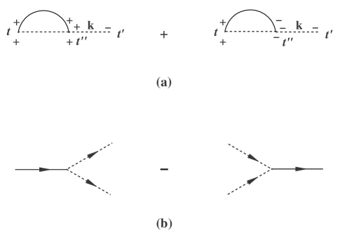
Figure 4.2: (a) The Feynman diagrams that contribute to the quantum kinetic equation for the pion distribution function at one loop order. The solid line is the sigma meson propagator and the dashed line is the pion propagator. (b) The only contribution on-shell is the decay of a sigma meson into two pions minus the reverse process.

Just as in the scalar case, since the propagators entering in the perturbative expansion of the kinetic equation are in terms of the distribution functions at the initial time, the time integration can be done straightforwardly leading to the following equation:

$$\frac{d}{dt}n^{\pi}_{\mathbf{k}}(t)=\lambda^{2}\int_{-\infty}^{+\infty}d\omega\,\mathcal{R}_{\pi}[\omega,\mathbf{k};\mathcal{N}_{j}(t_{0})]\,\frac{\sin[(\omega-k)(t-t_{0})]}{\pi(\omega-k)},$$ (4.60)

where $\mathcal{R}_{\pi}[\omega,\mathbf{k};\mathcal{N}_{j}(t_{0})]$ is given by

$$\mathcal{R}_{\pi}[\omega,\mathbf{k};\mathcal{N}_{j}(t_{0})] = \frac{f_{\pi}^{2}}{k}\,\int\frac{d^{3}q}{(2\pi)^{3}}\frac{1}{q\,\omega_{\mathbf{p}}}\Bigl{[}\delta(\Delta\omega_{1})\,\mathcal{N}_{1}(t_{0})+\delta(\Delta\omega_{2})\,\mathcal{N}_{2}(t_{0})$$ (4.61)

$$+\,\delta(\Delta\omega_{3})\,\mathcal{N}_{3}(t_{0})+\delta(\Delta\omega_{4})\,\mathcal{N}_{4}(t_{0})\Bigr{]}.$$

Eq.(4.60) can be solved by direct integration over $t$ with the given initial condition at $t_{0}$, leading to

$$n^{\pi}_{\mathbf{k}}(t)=n^{\pi}_{\mathbf{k}}(t_{0})+\lambda^{2}\int_{-\infty}^{+\infty}d\omega\,\mathcal{R}_{\pi}[\omega,\mathbf{k};\mathcal{N}_{j}(t_{0})]\,\frac{1-\cos[(\omega-k)(t-t_{0})]}{\pi(\omega-k)^{2}}.$$ (4.62)

Potential secular term arises at large times when the resonant denominator in (4.62) vanishes, i.e., $\omega\approx k$. A detailed analysis reveals that $\mathcal{R}_{\pi}[\omega,\mathbf{k};\mathcal{N}_{j}(t_{0})]$ is regular at $\omega=k$, hence upon using (4.24) one finds that at intermediate asymptotic time $k(t-t_{0})\gg 1$, the time evolution of the pion distribution function reads

$$n^{\pi}_{\mathbf{k}}(t)=n^{\pi}_{\mathbf{k}}(t_{0})+\lambda^{2}\,\mathcal{R}_{\pi}[k,\mathbf{k};\mathcal{N}_{j}(t_{0})]\,(t-t_{0})+\mbox{nonsecular terms},$$ (4.63)

where $\mathcal{R}_{\pi}[k,\mathbf{k};\mathcal{N}_{j}(t_{0})]$ does not depend on $t_{0}$ explicitly.

At this point we would be tempted to follow the same steps as in the scalar case and introduce the dynamical renormalization of the pion distribution function. However, much in the same manner as the renormalization program in a theory with several coupling constants, in the case under consideration the $\boldsymbol{\pi}$ field and the $\sigma$ field are coupled. Therefore one must renormalize all of the distribution functions on the same footing. Hence our next task is to obtain the kinetic equations for the sigma meson distribution functions.

Sigma mesons

The field operator for the sigma meson and the corresponding conjugate momentum in the Heisenberg picture can be written as (in momentum space)

$$\sigma(\mathbf{k},t)=\frac{1}{\sqrt{2\omega_{\mathbf{k}}}}\left[a_{\sigma}(\mathbf{k},t)+a^{\dagger}_{\sigma}(-\mathbf{k},t)\right],\quad\Pi_{\sigma}(\mathbf{k},t)=-i\sqrt{\frac{\omega_{\mathbf{k}}}{2}}\left[a_{\sigma}(\mathbf{k},t)-a^{\dagger}_{\sigma}(-\mathbf{k},t)\right],$$ (4.64)

with $\omega_{\mathbf{k}}=\sqrt{k^{2}+m_{\sigma}^{2}}$. Again, for notational simplicity we suppress the pion isospin index. The expectation value of sigma meson number operator can be expressed in terms of $\sigma(\mathbf{k},t)$ and $\Pi_{\sigma}(\mathbf{k},t)$ as

$$n^{\sigma}_{\mathbf{k}}(t) = \langle a^{\dagger}_{\sigma}(\mathbf{k},t)a_{\sigma}(\mathbf{k},t)\rangle$$ (4.65)

$$= \frac{1}{2\omega_{\mathbf{k}}}\left[\left\langle\Pi_{\sigma}(\mathbf{k},t)\Pi_{\sigma}(-\mathbf{k},t)\right\rangle+\omega_{\mathbf{k}}^{2}\left\langle\sigma(\mathbf{k},t)\sigma(-\mathbf{k},t)\right\rangle\right]-\frac{1}{2}.$$

Using the Heisenberg equations of motion to leading order in $\lambda$, and requiring again that the tadpole diagrams are canceled by the proper choice of $v$, we obtain

$$\frac{d}{dt}n^{\sigma}_{\mathbf{k}}(t) = -\frac{3\lambda f_{\pi}}{\omega_{\mathbf{k}}}\lim_{t^{\prime}\rightarrow t}\frac{\partial}{\partial t^{\prime}}\int\frac{d^{3}q}{(2\pi)^{3/2}}\Bigl{[}\big{\langle}\pi^{+}(\mathbf{k}-\mathbf{q},t)\pi^{+}(\mathbf{q},t)\sigma^{-}(-\mathbf{k},t^{\prime})\big{\rangle}$$ (4.66)

$$+\,3\big{\langle}\sigma^{+}(\mathbf{k}-\mathbf{q},t)\sigma^{+}(\mathbf{q},t)\sigma^{-}(-\mathbf{k},t^{\prime})\big{\rangle}\Bigr{]},$$

where the factor three for the first term accounts for three isospin components of the pion field.

To $\mathcal{O}(\lambda)$ the right hand side of Eq. (4.66) vanishes identically. Fig. 4.3a depicts the one-loop Feynman diagrams that enter in the kinetic equation for the sigma meson to order $\lambda^{2}$. To the same order there will be the same type of two loops diagrams as in the self-interacting scalar theory studied in the previous section, but in the low temperature limit the two-loop diagrams will be suppressed with respect to the one-loop diagrams. Furthermore, in the low temperature limit, the focus of our attention here, only the pion loops will be important in the relaxation of the sigma mesons. A straightforward calculation leads to the following expression

$$\frac{d}{dt}n^{\sigma}_{\mathbf{k}}(t) = \frac{3\lambda^{2}f_{\pi}^{2}}{2\omega_{\mathbf{k}}}\,\int\frac{d^{3}q}{(2\pi)^{3}}\int^{t}_{t_{0}}dt^{\prime\prime}\biggl{[}\frac{1}{p\,q}\Bigl{(}\mathcal{N}^{\pi}_{1}(t_{0})\cos[\Delta\omega^{\pi}_{1}(t-t^{\prime\prime})]$$ (4.67)

$$+\,\mathcal{N}^{\pi}_{2}(t_{0})\cos[\Delta\omega^{\pi}_{2}(t-t^{\prime\prime})]+\mathcal{N}^{\pi}_{3}(t_{0})\cos[\Delta\omega^{\pi}_{3}(t-t^{\prime\prime})]$$

$$+\,\mathcal{N}^{\pi}_{4}(t_{0})\cos[\Delta\omega^{\pi}_{4}(t-t^{\prime\prime})]\Bigr{)}+\frac{9}{\omega_{\mathbf{q}}\,\omega_{\mathbf{p}}}\Bigl{(}\pi\rightarrow\sigma\Bigr{)}\biggr{]},$$

where $\mathbf{p=k+q}$,

$$\Delta\omega^{\pi(\sigma)}_{1}=\omega_{\mathbf{k}}+q~{}(\omega_{\mathbf{q}})+p~{}(\omega_{\mathbf{p}}),\quad\Delta\omega^{\pi(\sigma)}_{2}=\omega_{\mathbf{k}}+q~{}(\omega_{\mathbf{q}})-p~{}(\omega_{\mathbf{p}}),$$

$$\Delta\omega^{\pi(\sigma)}_{3}=\omega_{\mathbf{k}}-q~{}(\omega_{\mathbf{q}})+p~{}(\omega_{\mathbf{p}}),\quad\Delta\omega^{\pi(\sigma)}_{4}=\omega_{\mathbf{k}}-q~{}(\omega_{\mathbf{q}})-p~{}(\omega_{\mathbf{p}}),$$ (4.68)

and

$$\mathcal{N}^{\pi(\sigma)}_{1}(t) = [1+n^{\sigma}_{\mathbf{k}}(t)][1+n^{\pi(\sigma)}_{\mathbf{q}}(t)][1+n^{\pi(\sigma)}_{\mathbf{p}}(t)]-n^{\sigma}_{\mathbf{k}}(t)\,n^{\pi(\sigma)}_{\mathbf{q}}(t)\,n^{\pi(\sigma)}_{\mathbf{p}}(t),$$

$$\mathcal{N}^{\pi(\sigma)}_{2}(t) = [1+n^{\sigma}_{\mathbf{k}}(t)][1+n^{\pi(\sigma)}_{\mathbf{q}}(t)]n^{\pi(\sigma)}_{\mathbf{p}}(t)-n^{\sigma}_{\mathbf{k}}(t)\,n^{\pi(\sigma)}_{\mathbf{q}}(t)\,[1+n^{\pi(\sigma)}_{\mathbf{p}}(t)],$$

$$\mathcal{N}^{\pi(\sigma)}_{3}(t) = [1+n^{\sigma}_{\mathbf{k}}(t)]\,n^{\pi(\sigma)}_{\mathbf{q}}(t)\,[1+n^{\pi(\sigma)}_{\mathbf{p}}(t)]-n^{\sigma}_{\mathbf{k}}(t)\,[1+n^{\pi(\sigma)}_{\mathbf{q}}(t)]\,n^{\pi(\sigma)}_{\mathbf{p}}(t),$$

$$\mathcal{N}^{\pi(\sigma)}_{4}(t) = [1+n^{\sigma}_{\mathbf{k}}(t)]\,n^{\pi(\sigma)}_{\mathbf{q}}(t)\,n^{\pi(\sigma)}_{\mathbf{p}}(t)-n^{\sigma}_{\mathbf{k}}(t)\,[1+n^{\pi(\sigma)}_{\mathbf{q}}(t)][1+n^{\pi(\sigma)}_{\mathbf{p}}(t)].$$ (4.69)

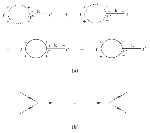
Figure 4.3: (a) The Feynman diagrams that contribute to the quantum kinetic equation for the sigma meson distribution function at one-loop order. The solid line is the sigma meson propagator and the dashed line is the pion propagator. (b) The only contribution on-shell is recombination of two pions into a sigma meson minus the decay of a sigma meson into two pions.

Although the above expression is somewhat unwieldy, the different contributions have a very natural interpretation in terms of the “gain minus loss” processes. In the first parentheses (the pion contribution) the first term corresponds to the process $0\rightarrow\sigma+\pi+\pi$ minus the process $\sigma+\pi+\pi\rightarrow 0$, the second and third terms correspond to the scattering $\pi\rightarrow\pi+\sigma$ minus $\pi+\sigma\rightarrow\pi$, and the last term corresponds to the decay of the sigma meson $\sigma\rightarrow\pi+\pi$ minus the inverse process $\pi+\pi\rightarrow\sigma$. Likewise, in the second parentheses (the sigma meson contribution) the first term corresponds to the process $0\rightarrow\sigma+\sigma+\sigma$ minus the process $\sigma+\sigma+\sigma\rightarrow 0$, the second and third terms correspond to annihilation of two sigma mesons and creation of one sigma meson minus the inverse process, and the last term corresponds to annihilation of a sigma meson and creation of two sigma mesons minus the inverse process.

Since the propagators entering in the perturbative expansion of the kinetic equation are in terms of the distribution functions at the initial time, the time integration can be done straightforwardly leading to the following equation:

$$\frac{d}{dt}n^{\sigma}_{\mathbf{k}}(t)=\lambda^{2}\int_{-\infty}^{+\infty}d\omega\,\mathcal{R}_{\sigma}[\omega,\mathbf{k};\mathcal{N}_{j}(t_{0})]\,\frac{\sin[(\omega-\omega_{\mathbf{k}})(t-t_{0})]}{\pi(\omega-\omega_{\mathbf{k}})},$$ (4.70)

where

$$\mathcal{R}_{\sigma}[\omega,\mathbf{k};\mathcal{N}_{j}(t_{0})] = \frac{3f_{\pi}^{2}}{2\omega_{\mathbf{k}}}\,\int\frac{d^{3}q}{(2\pi)^{3}}\biggl{[}\frac{1}{p\,q}\Bigl{(}\delta(\Delta\omega^{\pi}_{1})\,\mathcal{N}^{\pi}_{1}(t_{0})+\delta(\Delta\omega^{\pi}_{2})\,\mathcal{N}^{\pi}_{2}(t_{0})+\delta(\Delta\omega^{\pi}_{3})$$ (4.71)

$$\times\,\mathcal{N}^{\pi}_{3}(t_{0})+\delta(\Delta\omega^{\pi}_{4})\,\mathcal{N}^{\pi}_{4}(t_{0})\Bigr{)}+\frac{9}{\omega_{\mathbf{q}}\,\omega_{\mathbf{p}}}\Bigl{(}\pi\rightarrow\sigma\Bigr{)}\biggr{]}.$$

Just as before $\mathcal{R}_{\sigma}[\omega,\mathbf{k};\mathcal{N}_{j}(t_{0})]$ is fixed at initial time $t_{0}$, Eq. (4.70) can be integrated over $t$ with the given initial condition at $t_{0}$, thus leading to

$$n^{\sigma}_{\mathbf{k}}(t)=n^{\sigma}_{\mathbf{k}}(t_{0})+\lambda^{2}\int_{-\infty}^{+\infty}d\omega\,\mathcal{R}_{\sigma}[\omega,\mathbf{k};\mathcal{N}_{j}(t_{0})]\frac{1-\cos[(\omega-\omega_{\mathbf{k}})(t-t_{0})]}{\pi(\omega-\omega_{\mathbf{k}})^{2}}.$$ (4.72)

At intermediate asymptotic times $m_{\sigma}(t-t_{0})\gg 1$, potential secular term arises when $\omega\approx\omega_{\mathbf{k}}$ in Eq. (4.72). We notice that, although $\mathcal{R}_{\sigma}[\omega,\mathbf{k};\mathcal{N}_{j}(t_{0})]$ has (infrared) threshold singularities at $\omega=\pm k$, it is regular on the sigma meson mass shell. This observation will allow us to explore a crossover behavior for very large momentum later.

Since $\mathcal{R}_{\sigma}[\omega,\mathbf{k};\mathcal{N}_{j}(t_{0})]$ is regular near the resonance region $\omega=\pm\omega_{\mathbf{k}}$, the behavior at intermediate asymptotic times is given by

$$n^{\sigma}_{\mathbf{k}}(t)=n^{\sigma}_{\mathbf{k}}(t_{0})+\lambda^{2}\,\mathcal{R}_{\sigma}[\omega_{\mathbf{k}},\mathbf{k};\mathcal{N}_{j}(t_{0})](t-t_{0})+\mbox{nonsecular terms}.$$ (4.73)

We note that the perturbative expansions for the pion and sigma meson distribution functions contain secular terms that grow linearly in time, unless the system is initially prepared in thermal equilibrium. To resum the secular terms, we must now renormalize both Eqs. (4.63) and (4.73) simultaneously, because, as discussed in Sec. 4.3, this situation corresponds to that with two relevant couplings in Euclidean field theory. The renormalization is achieved by introducing the renormalized initial distribution functions $n^{\pi(\sigma)}_{\mathbf{k}}(\tau)$ for pions (sigma mesons) that are related to the bare initial distribution functions $n^{\pi(\sigma)}_{\mathbf{k}}(t_{0})$ via the renormalization constants $\mathcal{Z}^{\pi(\sigma)}_{\mathbf{k}}(\tau,t_{0})$

$$n^{\pi(\sigma)}_{\mathbf{k}}(t_{0})=\mathcal{Z}^{\pi(\sigma)}_{\mathbf{k}}(\tau,t_{0})\,n^{\pi(\sigma)}_{\mathbf{k}}(\tau),\quad\mathcal{Z}^{\pi(\sigma)}_{\mathbf{k}}(\tau,t_{0})=1+\lambda^{2}\,z^{\pi(\sigma)}_{\mathbf{k}}(\tau,t_{0})+\mathcal{O}(\lambda^{4}),$$ (4.74)

where $\tau$ is an arbitrary renormalization scale at which the secular terms will be canceled. As in the case of the scalar theory, the renormalization constants $z^{\pi(\sigma)}_{\mathbf{k}}(\tau,t_{0})$ are chosen so as to cancel the secular terms at the arbitrary scale $\tau$. Upon substitute Eq. (4.74) into Eq. (4.63) and choosing

$$z^{\pi(\sigma)}_{\mathbf{k}}(\tau,t_{0})=-(\tau-t_{0})\frac{\mathcal{R}_{\pi(\sigma)}[k,\mathbf{k};\mathcal{N}_{j}(\tau)]}{n^{\pi(\sigma)}_{\mathbf{k}}(\tau)},$$ (4.75)

consistently up to $\mathcal{O}(\lambda^{2})$, one obtains

$$n^{\pi(\sigma)}_{\mathbf{k}}(t)=n^{\pi(\sigma)}_{\mathbf{k}}(\tau)+\lambda^{2}\,(t-\tau)\,\mathcal{R}_{\pi(\sigma)}[k\,(\omega_{\mathbf{k}}),\mathbf{k};\mathcal{N}_{j}(\tau)]+\mathcal{O}(\lambda^{4}).$$ (4.76)

The independence of $n^{\pi(\sigma)}_{\mathbf{k}}(t)$ on the arbitrary renormalization scale $\tau$ leads to the simultaneous set of dynamical renormalization group equations to lowest order:

$$\frac{d}{d\tau}n^{\pi}_{\mathbf{k}}(\tau)=\lambda^{2}\,\mathcal{R}_{\pi}[k,\mathbf{k};\mathcal{N}_{j}(\tau)],$$

$$\frac{d}{d\tau}n^{\sigma}_{\mathbf{k}}(\tau)=\lambda^{2}\,\mathcal{R}_{\sigma}[\omega_{\mathbf{k}},\mathbf{k};\mathcal{N}_{j}(\tau)].$$ (4.77)

These equations have an obvious resemblance to a set of usual renormalization group equations for “couplings” $n^{\pi}_{\mathbf{k}}$ and $n^{\sigma}_{\mathbf{k}}$, where the right-hand sides are the corresponding “beta functions”.

As before choosing the arbitrary scale $\tau$ to coincide with the time $t$ and keeping only the terms whose delta functions have support on the mass shells, we obtain the quantum kinetic equations for pions and sigma mesons:

$$\frac{d}{dt}n^{\pi}_{\mathbf{k}}(t)\!\! = \!\!\frac{\pi\lambda^{2}f_{\pi}^{2}}{k}\,\int\frac{d^{3}q}{(2\pi)^{3}}\frac{\delta(k+q-\omega_{\mathbf{p}})}{q\,\omega_{\mathbf{p}}}\Big{\{}[1+n^{\pi}_{\mathbf{k}}(t)][1+n^{\pi}_{\mathbf{q}}(t)]\,n^{\sigma}_{\mathbf{p}}(t)$$ (4.78)

$$-\,n^{\pi}_{\mathbf{k}}(t)\,n^{\pi}_{\mathbf{q}}(t)\,[1+n^{\sigma}_{\mathbf{p}}(t)]\Big{\}},$$

$$\frac{d}{dt}n^{\sigma}_{\mathbf{k}}(t)\!\! = \!\!\frac{3\pi\lambda^{2}f_{\pi}^{2}}{2\omega_{\mathbf{k}}}\,\int\frac{d^{3}q}{(2\pi)^{3}}\frac{\delta(\omega_{\mathbf{k}}-q-p)}{p\,q}\Big{\{}[1+n^{\sigma}_{\mathbf{k}}(t)]\,n^{\pi}_{\mathbf{q}}(t)\,n^{\pi}_{\mathbf{p}}(t)$$ (4.79)

$$-\,n^{\sigma}_{\mathbf{k}}(t)\,[1+n^{\pi}_{\mathbf{q}}(t)][1+n^{\pi}_{\mathbf{p}}(t)]\Big{\}}.$$

The processes that contribute to Eq. (4.78) are depicted in Fig. 2b and those that contribute to Eq. (4.79) are depicted in Fig. 3b.

4.4.2 Relaxation rate for pions and sigma mesons

Thermal equilibrium is a fixed point of the dynamical renormalization group equations, i.e., a stationary solution of the quantum kinetic equations (4.78) and (4.79). Near equilibrium a Linearized kinetic equation for pions (sigma mesons) can be obtained in the relaxation time approximation, in which only distribution function for pions (sigma mesons) of momentum $\mathbf{k}$ are slightly perturbed off equilibrium whereas all the other modes are in equilibrium. In the relaxation time approximation for pions (sigma mesons), one obtains

$$\frac{d}{dt}\delta n^{\pi(\sigma)}_{\mathbf{k}}(t)=-\Gamma_{\pi(\sigma)}(k)\,\delta n^{\pi(\sigma)}_{\mathbf{k}}(t),$$ (4.80)

where $\Gamma_{\pi(\sigma)}(k)$ is the pion (sigma meson) relaxation rate, which is identified with twice the damping rate of the corresponding mean field.

Linearizing Eq. (4.78) in the relaxation time approximation, we obtain the pion relaxation rate to be given by

$$\Gamma_{\pi}(k) = \frac{\pi\lambda^{2}f_{\pi}^{2}}{k}\,\int\frac{d^{3}q}{(2\pi)^{3}}\frac{n_{B}(q)-n_{B}(\omega_{\mathbf{p}})}{q\,\omega_{\mathbf{p}}}\,\delta(k+q-\omega_{\mathbf{p}})$$ (4.81)

$$= \frac{\lambda^{2}f_{\pi}^{2}T}{4\pi k^{2}}\,\ln\frac{1-e^{-\beta(m_{\sigma}^{2}/4k+k)}}{1-e^{-\beta m_{\sigma}^{2}/4k}}.$$

This is a remarkable expression because it reveals that the physical processes that contribute to pion relaxation are the decay of a sigma meson to two pions and its inverse process, i.e., $\sigma\rightleftarrows\pi+\pi$. The sigma mesons present in the medium can decay into pions and this increases the number of pions, but at the same time pions recombine into sigma mesons, and since there are more pions in the medium because they are lighter the loss part of the process prevails producing a non-zero relaxation rate for the pion distribution function. This is an induced phenomenon in the medium in the very definitive sense that the decay of the heavier sigma meson induces the relaxation of the pion distribution function, it is a collisionless process. We note that such induced relaxation of pions is analogous to the relaxation of fermions in a fermion-scalar plasma discusses in Chap. 3, the latter is induced by the decay of a massive scalar into light fermion pairs.

For soft, cool pions $(k\ll T\ll f_{\pi})$, the relaxation rate reads

$$\gamma_{\pi}(k\ll T)\approx\frac{\lambda^{2}f_{\pi}^{2}}{4\pi k}\exp\left(-\frac{m_{\sigma}^{2}}{4kT}\right).$$ (4.82)

The exponential suppression in the above expression is a consequence of the heavy sigma mass. Our results of the pion relaxation rate are in agreement with the pion damping rate found in Ref. [98]. These results (accounting for the factor two necessary to relate the relaxation rate to the damping rate) also agree with those reported recently in Ref. [99], wherein a related and clear analysis of pion and sigma meson damping rates was presented.

Likewise, the sigma meson relaxation rate in the relaxation time approximation is found to be given by

$$\Gamma_{\sigma}(k) = \frac{3\pi\lambda^{2}f_{\pi}^{2}}{2\omega_{\mathbf{k}}}\,\int\frac{d^{3}q}{(2\pi)^{3}}\frac{\left[1+n_{B}(q)+n_{B}(p)\right]}{p\,q}\,\delta(\omega_{\mathbf{k}}-q-p)$$ (4.83)

$$= \frac{3\lambda^{2}f_{\pi}^{2}}{8\pi\omega_{\mathbf{k}}}\left[1+\frac{2T}{k}\,\ln\frac{1-e^{-\beta(\omega_{\mathbf{k}}+k)/2}}{1-e^{-\beta(\omega_{\mathbf{k}}-k)/2}}\right].$$

We note that the first temperature-independent term in $\Gamma_{\sigma}(k)$ is the usual zero-temperature sigma meson decay rate [100], whereas the finite-temperature terms result from the same processes $\sigma\rightleftarrows\pi+\pi$ that also determine $\Gamma_{\pi}(k)$. For soft, cool sigma meson ($k\ll T\ll f_{\pi}$), one obtains

$$\Gamma_{\sigma}({k\approx 0})\approx\frac{3\lambda^{2}f_{\pi}^{2}}{8\pi m_{\sigma}}\coth\left(\frac{m_{\sigma}}{4T}\right),$$ (4.84)

which agrees with the decay rate for a sigma meson at rest [99, 101, 102].

On the other hand, let us consider the theoretical high temperature and large momentum limit $k\gg m_{\sigma}\gtrsim T$ and $\omega_{\mathbf{k}}-k\ll T$. In this limit $\Gamma_{\sigma}(k)$ becomes logarithmic (infrared) divergent. The reason for this divergence is that, as was mentioned above, $\mathcal{R}_{\sigma}[\omega,\mathbf{k};\mathcal{N}_{j}(t_{0})]$ has an infrared threshold singularity at $\omega=k$ arising from the terms proportional to $\mathcal{N}^{\pi}_{4}(t_{0})$, which accounts for the emission and absorption of collinear massless pions. In the presence of this threshold singularity, we can no longer apply Fermi’s golden rule (4.24). Instead, we must analyze the long-time behavior of Eq. (4.67) more carefully.

Understanding the influence of threshold behavior of the sigma meson on its relaxation could be important in view of the recent proposal by Hatsuda and collaborators [89] that near the chiral phase transition the mass of the sigma meson drops and threshold effects become enhanced with distinct phenomenological consequences.

4.4.3 Threshold singularities and crossover in relaxation

In order to understand how the (infrared) threshold divergence modifies the long-time behavior, let us focus on the sigma mesons with large momentum $k\gg m_{\sigma}\gtrsim T$. This situation is not relevant to the phenomenology of the cool pion-sigma meson system for which relevant temperatures are $T\ll m_{\sigma}$. However studying this theoretical limiting case will reveal important insight on how threshold divergences invalidate the usual Fermi’s golden rule analysis, which leads to energy conservation delta functions in the intermediate asymptotic regimes. This issue will become physical relevant in the case of gauge field theories studied below (see Chap. 5).

To present this case in the simplest and clearest manner, we will proceed in the relaxation time approximation. Keeping only the infrared divergent contribution in $\mathcal{R}_{\sigma}[\omega,\mathbf{k};\mathcal{N}_{j}(t_{0})]$, i.e., the term proportional to $\mathcal{N}^{\pi}_{4}(t_{0})$, one finds that Eq. (4.72) simplifies to

$$\delta n^{\sigma}_{\mathbf{k}}(t)=\delta n^{\sigma}_{\mathbf{k}}(t_{0})\left[1-\int_{-\infty}^{+\infty}d\omega\,\mathcal{R}(\omega,\mathbf{k})\,\frac{1-\cos[(\omega-\omega_{\mathbf{k}})(t-t_{0})]}{\pi(\omega-\omega_{\mathbf{k}})^{2}}\right],$$ (4.85)

where

$$\mathcal{R}(\omega,\mathbf{k}) = \frac{3\pi\lambda^{2}f_{\pi}^{2}}{2\omega_{\mathbf{k}}}\,\int\frac{d^{3}q}{(2\pi)^{3}}\,\frac{1+n_{B}(q)+n_{B}(p)}{p\,q}\,\delta(\omega-q-p)$$ (4.86)

$$= \frac{3\lambda^{2}f_{\pi}^{2}}{8\pi\omega_{\mathbf{k}}}\left[1+\frac{2T}{k}\,\ln\frac{1-e^{-\beta(\omega+k)/2}}{1-e^{-\beta(\omega-k)/2}}\right],$$

which has a infrared threshold singularity at $\omega=k$. At intermediate asymptotic times $m_{\sigma}(t-t_{0})\gg 1$, the integral over $\omega$ in Eq.(4.85) is dominated by the region near $\omega\approx k$. In the limit $k\gg m_{\sigma}\gtrsim T$, by approximating

$$\mathcal{R}(\omega,\mathbf{k})\,\buildrel\omega\to k\over{=}\,\frac{3\lambda^{2}f_{\pi}^{2}T}{4\pi k^{2}}\,\ln\left[\frac{2T}{\omega-k}\right]+\mathcal{O}(\omega-k),$$ (4.87)

the $\omega$ integral (denoted as $\mathcal{I}$) for $m_{\sigma}(t-t_{0})\gg 1$ can be evaluated in a closed form

$$\mathcal{I}\approx\frac{3\lambda^{2}f_{\pi}^{2}\bar{T}}{4\pi k^{2}}\,\mathcal{F}(\bar{t}),$$ (4.88)

where $\bar{T}=T/(\omega_{\mathbf{k}}-k)\approx 2kT/m_{\sigma}^{2}$ and $\bar{t}=(\omega_{\mathbf{k}}-k)(t-t_{0})\approx m_{\sigma}^{2}(t-t_{0})/2k$ are dimensionless variables and

$$\mathcal{F}(x)=x\left(\ln 2\bar{T}+\mathrm{ci}(x)-\frac{\sin x}{x}\right),$$ (4.89)

with $\mathrm{ci}(x)$ being the cosine integral function

$$\mathrm{ci}(x)=-\int_{x}^{+\infty}dt\,\frac{\cos t}{t}.$$ (4.90)

The function $\mathcal{F}(x)$ has the following asymptotic behaviors

$$\mathcal{F}(x)=\left\{\begin{array}[]{ll}x\left[\ln 2x\bar{T}+\gamma-1+\mathcal{O}\left(x^{2}\right)\right]&\quad\mathrm{for}\quad x\ll 1,\\ x\left[\ln 2\bar{T}+\mathcal{O}\left(x^{-2}\right)\right]&\quad\mathrm{for}\quad x\gg 1,\end{array}\right.$$ (4.91)

where $\gamma=0.577\ldots$ is the Euler-Mascheroni constant. Thus, for fixed and large $k$ one can see that there is a crossover time scale $t_{c}\approx 2k/m_{\sigma}^{2}$ on which the time dependence of $\mathcal{F}(\bar{t})$ changes from the $t\ln t$ dependence for $t-t_{0}\ll t_{c}$ to the linear dependence for $t-t_{0}\gg t_{c}$. Consequently, in the large momentum limit as the sigma meson mass shell approaches the threshold, this crossover time scale becomes very long such that an “anomalous” (nonlinear) secular term of the form $t\ln t$ dominates during most of the time whereas the usual linear secular term ensues at very large times.

The secular terms can be resumed by implementing the dynamical renormalization group method [see Eq. (4.73)] with the following choice of renormalization constant (in terms of dimensionless time variable)

$$z^{\sigma}_{\mathbf{k}}(\tau,\bar{t}_{0})=\frac{3f_{\pi}^{2}\bar{T}}{4\pi k^{2}}\,\mathcal{F}(\tau-\bar{t}_{0}).$$ (4.92)

The resultant dynamical renormalization group equation reads

$$\frac{d}{d\bar{t}}\,\delta n^{\sigma}_{\mathbf{k}}(\bar{t})+\frac{3\lambda^{2}f_{\pi}^{2}\bar{T}}{4\pi k^{2}}\,\frac{d}{d\bar{t}}\,\mathcal{F}(\bar{t}-\bar{t}_{0})=0,$$ (4.93)

whose solution is given by

$$\delta n^{\sigma}_{\mathbf{k}}(\bar{t})=\delta n^{\sigma}_{\mathbf{k}}(\bar{t}_{0})\exp\left[-\frac{3\lambda^{2}f_{\pi}^{2}\bar{T}}{4\pi k^{2}}\mathcal{F}(\bar{t}-\bar{t}_{0})\right].$$ (4.94)

In the large momentum limit, using Eq. (4.91) we find that the crossover in the form of the secular terms results in a crossover in the sigma meson relaxation: an “anomalous” (nonexponential) relaxation will dominate during most of the time and the usual exponential relaxation ensues at very large times.

This above discussion has revealed several important features highlighted by a consistent resummation via the dynamical renormalization group:

(i) Threshold infrared divergences result in a breakdown of Fermi’s golden rule. The secular terms of the perturbative expansion are no longer linear in time but include logarithmic contributions arising from these infrared divergences.

(ii) The concept of the damping rate is directly tied to exponential relaxation. The infrared divergences of the damping rate reflect the breakdown of Fermi’s golden rule and signal a very different relaxation from a simple exponential.

(iii) Whereas the usual calculation of damping rates will lead to a divergent result arising from the infrared threshold divergences, the dynamical renormalization group approach recognizes that these threshold divergences result in secular terms that are non-linear in time as discussed above. While in relaxation time approximation linear secular terms lead to exponential relaxation and therefore to an unambiguous definition of the damping rate, non-linear secular terms lead to novel nonexponential relaxation phenomena for which the concept of a damping rate may not be appropriate.

This discussion of threshold singularities and anomalous relaxation has paved the way to studying the case of gauge field theories in next chapter, wherein the emission and absorption of magnetic photons that are only dynamically screened lead to a similar anomalous relaxation [84].

4.5 Pinch Singularities and their Resolution

An important difference between the approach to nonequilibrium evolution described by quantum kinetic equations advocated in this work and that often presented in the literature is that we work directly in real time not taking Fourier transforms in time. This has to be contrasted with the so-called real-time formalism (RTF) of (non)equilibrium quantum field theory, in which there are also a closed-time-path contour and four propagators but the propagators and quantities computed therefrom are all in terms of temporal Fourier transforms.

In thermal equilibrium the Fourier representation of these four propagators for a scalar field are given by [43, 37, 87]

$$G_{0}^{++}(K)=-G_{0}^{--}(K)^{\ast}=-\frac{1}{K^{2}-m^{2}_{\mathrm{eff}}+i\varepsilon}+2\pi in_{B}(|k_{0}|)\,\delta(K^{2}-m^{2}_{\mathrm{eff}}),$$

$$G_{0}^{-+}(K)=2\pi i\,[\theta(k_{0})+n_{B}(|k_{0}|)]\,\delta(K^{2}-m^{2}_{\mathrm{eff}}),$$

$$G_{0}^{+-}(K)=2\pi i\,[\theta(-k_{0})+n_{B}(|k_{0}|)]\,\delta(K^{2}-m^{2}_{\mathrm{eff}}),$$ (4.95)

where $K=(k_{0},\mathbf{k})$ is the four-momentum with $K^{2}=k_{0}^{2}-k^{2}$, whereas out of equilibrium the distribution functions are simply replaced by non-thermal ones, i.e., $n_{B}(|k_{0}|)\rightarrow n_{\mathbf{k}}(t_{0})$. Using the integral representation of the Heaviside step function

$$\theta(t)=\frac{i}{2\pi}\int_{-\infty}^{+\infty}\frac{d\omega}{\omega+i\varepsilon}\,e^{-i\omega t},$$ (4.96)

one can easily show that the propagators given in Eq. (4.95) and the ones obtained by replacing the thermal equilibrium distributions by the nonequilibrium ones are, respectively, the temporal Fourier transforms of those given in Eqs. (3.5) and (4.2). The Fourier transforms of the free retarded and advanced propagators are obtained similarly and read

$$G_{0}^{R/A}(K)=-\frac{1}{K^{2}-m^{2}_{\mathrm{eff}}\pm i\,\textrm{sgn}(k_{0})\,\varepsilon}.$$ (4.97)

Several authors have pointed out that the calculations using the CTP formalism in terms of the standard form of free propagators in Eq. (4.95) or those obtained by the replacement of the distribution functions by the nonequilibrium ones, lead to pinch singularities [87, 88, 103, 104, 105, 106, 107].

In a consistent perturbative expansion both the retarded and advanced propagators contribute and pinch singularities arise from the product of these, for example for a scalar field this product is of the form

$$G_{0}^{R}(K)\,G_{0}^{A}(K)=\frac{1}{[K^{2}-m^{2}_{\mathrm{eff}}+i\,\textrm{sgn}(k_{0})\,\varepsilon][K^{2}-m^{2}_{\mathrm{eff}}-i\,\textrm{sgn}(k_{0})\,\varepsilon]}.$$ (4.98)

For finite $\varepsilon$ this expression is regular, whereas when $\varepsilon\rightarrow 0^{+}$ it gives rise to singular products such as $[\delta(K^{2}-m^{2}_{\mathrm{eff}})]^{2}$ as discussed in Refs. [87, 88, 103, 104, 105, 106, 107]. Singularities of this type are ubiquitous in nonequilibrium and are not particular to scalar field theories.

A detailed analysis of these pinch terms reveals that they do not cancel each other in perturbation theory unless the system is in thermal equilibrium [87, 88, 103, 104, 105]. Indeed, this severe problem has cast doubt on the validity or usefulness of the CTP formulation to describe nonequilibrium phenomena [88]. Although this singularities have been found in many circumstances and analyzed and discussed in the literature often, a systematic and satisfactory treatment of these singularities is still lacking. In Ref. [107] it was suggested that including an in-medium width of the quasiparticles to replace Feynman’s “$i\varepsilon$-prescription” does provide a physically reasonable solution, however this clearly casts doubt on the consistency of any perturbative approach to describe even weakly out of equilibrium phenomena.

Recently some authors have conjectured that pinch singularities in perturbation theory might be attributed to a misuse of Fourier transforms (for a detailed discussion see Refs. [103, 104, 105]). As an illustrative and simple example of these type of pinch singularities, these authors discussed the elementary derivation of Fermi’s golden rule in time-dependent perturbation theory in quantum mechanics. In calculating total transition probabilities there appears the square of energy conservation delta function, which arises due to taking the infinite time limit of scattering probabilities. In this setting, such terms are interpreted as the elapsed scattering time multiplied by the energy conservation constraint rather than a pathological singularity.

A close inspection of Eq. (4.98) reveals that the pinch term is the square of on-shell condition for the free quasiparticle, which implies a temporal Fourier transform in the infinite time limit and of the same form as the square of the energy conservation constraint for the transition probability obtained in time-dependent perturbation theory.

By assuming that the interaction duration time is large but finite, Niégawa [104] and Greiner and Leupold [105] showed that for a self-interacting scalar field the pinch part of the distribution function can be regularized by the interaction duration time as [104, 105]

$$n^{\mathrm{pinch}}_{\mathbf{k}}(t)\simeq(t-t_{0})\,\Gamma^{\mathrm{net}}_{\mathbf{k}}(t_{0}),$$ (4.99)

where “$\simeq$” denotes that only the pinch singularity contribution is included, $t-t_{0}$ is the interaction duration time, and $\Gamma^{\mathrm{net}}_{\mathbf{k}}(t_{0})$ is the net gain rate of the quasiparticle distribution function per unit time

$$\Gamma^{\mathrm{net}}_{\mathbf{k}}(t_{0})=\frac{i}{2\omega_{\mathbf{k}}}\Big{[}[1+n_{\mathbf{k}}(t_{0})]\Sigma^{<}(\omega_{\mathbf{k}},\mathbf{k})-n_{\mathbf{k}}(t_{0})\Sigma^{>}(\omega_{\mathbf{k}},\mathbf{k})\Big{]}.$$ (4.100)

In the above expression, the on-shell self-energies $\Sigma^{\gtrless}(\omega_{\mathbf{k}},\mathbf{k})$ are calculated in terms of the initial distribution functions $n_{\mathbf{k}}(t_{0})$ [104, 105].

Upon comparing Eqs. (4.99) and (4.100) with Eqs. (4.25) and (4.28), respectively, we clearly see the equivalence between the linear secular terms in the perturbative expansion and the presence of pinch singularities in the usual CTP formalism. Furthermore, in the discussion following Eq.(4.25) we have recognized that secular terms are not present if the system is in equilibrium, much in the same manner as the case of pinch singularities as discussed originally by Altherr [88]. Thus our conclusion is that pinch singularities are a temporal Fourier transform representation of linear secular terms.

The dynamical renormalization group provides a systematic resummation of these secular terms and a consistent formulation to implement the renormalization of the distribution functions suggested by Niégawa. [104]. We emphasize that the dynamical renormalization group approach explains the physical origin of the pinch singularities in terms of secular terms and Fermi’s golden rule, and provides a consistent and systematic resummation of these secular terms that lead to the quantum kinetic equation as a renormalization group equation that determines the time evolution of the distribution function. This result justifies in a systematic manner the conclusions and interpretation obtained in Ref. [107] where a possible regularization of the pinch singularities was achieved by including the width of the quasiparticle obtained via the resummation of hard thermal loops.

Furthermore, we stress that the dynamical renormalization group is far more general in that it allows to treat situations where the long time evolution is modified by threshold (infrared) singularities in spectral densities, thereby providing a resolution of infrared singularities in damping rates and a consistent resummation scheme to extract the asymptotic time evolution of the distribution function. The infrared singularities in these damping rates is a reflection of anomalous (nonexponential) relaxation as a result of threshold effects.

The pinch singularities signal the breakdown of perturbation theory, just as the secular terms in real time, however, the advantage of working directly in real time is that the time scale on which perturbation theory breaks down is recognized clearly from the real-time perturbative expansion and is identified directly with the kinetic time scale. The dynamical renormalization group justifies this identification by providing a resummation of the perturbative series that improves the solution beyond the intermediate asymptotics.

The resolution of pinch singularities via the dynamical renormalization group is general. As originally pointed out in Ref. [88] the pinch singularities typically multiply expressions of the form Eq. (4.100) which vanish in equilibrium, just as the linear secular terms multiply similar terms in the real-time perturbative expansion, as highlighted by Eq. (4.28). These terms are of the typical form gain minus loss, in equilibrium they vanish, but their nonvanishing simply indicates that the distribution functions are evolving in time and it is precisely this time evolution that is described consistently by the dynamical renormalization group.

4.6 Conclusions

The goal of this chapter is to provide a novel method for obtaining quantum kinetic equations from a field theoretical and diagrammatic perturbative expansion that is improved via a dynamical renormalization group resummation directly in real time.

The first step of this method is to use the microscopic equations of motion to obtain the evolution equation of the quasiparticle distribution function, i.e., the expectation value of the quasiparticle number operator in the initial density matrix. This evolution equation can be solved in a consistent diagrammatic perturbative expansion and one finds that the solution for the time evolution of the distribution function features secular terms, i.e., terms that grow in time. In perturbation theory the microscopic and kinetic time scales are widely separated, hence there is a regime of intermediate asymptotics in time, within which (i) perturbation theory is valid and (ii) the secular terms dominate the time evolution of the distribution function.

The second step is to implement the dynamical renormalization group to resum the secular terms. A renormalization of the distribution function absorbs the contribution from the secular terms on a given renormalization time scale, thereby improving the perturbative expansion. The arbitrariness of this renormalization scale leads to the dynamical renormalization group equation, which is interpreted as the quantum kinetic equation. In relaxation time approximation linear one recognizes that secular terms correspond to usual exponential relaxation, whereas nonlinear secular terms correspond to anomalous (nonexponential) relaxation.

We first test this new dynamical renormalization group method within the familiar self-interacting scalar field theory, not only reproducing but also generalizing the previous results in the literature. We then move on to apply the this method to study quantum kinetics of a gas of cool pions and sigma mesons described by the $O(4)$ linear sigma model in the chiral limit. In the relaxation time approximation the exponential relaxation of the pions and sigma mesons is described by the corresponding relaxation rates, which are in agreement with the damping rate found recently for the same model [98, 99, 102]. This particular model also reveals a crossover behavior in sigma meson relaxation in the large momentum limit as a result of threshold singularities associated with the emission and absorption of massless pions. In the relaxation time approximation we find a crossover between purely exponential and anomalous nonexponential relaxation with an exponent of the form $t\ln t$. The crossover time scale is found to be dependant on the momentum of the sigma resonance. The anomalous relaxation is a novel result and could be of phenomenological relevance in view of recent suggestions of novel threshold effects of the sigma resonance near the chiral phase transition [89], this possibility is worthy of a deeper study and generalization of the dynamical renormalization group method to reach the critical region is in progress.

Furthermore, we have established a very close relationship between the usual renormalization group and the dynamical renormalization group approach to kinetics. We have shown that the dynamical renormalization group equation is the quantum kinetic equation, the collision terms are the equivalent of the beta functions in the Euclidean renormalization group. Fixed points of the dynamical renormalization group are identified with stationary solutions of the kinetic equation and the exponents that determine the stability of the fixed points are identified with the relaxation rates in the relaxation time approximation. We have also suggested that in this language coarse-graining is the equivalent to neglecting irrelevant couplings in the Euclidean renormalization program. This identification brings a new and rather different perspective to kinetics and relaxation that will hopefully lead to new insights.

There are many advantages in the dynamical renormalization group approach to quantum kinetics:

(i) This method is based on straightforward quantum field theoretical diagrammatic perturbation, hence it allows a systematic calculation to any arbitrary order in perturbation theory. It includes nonequilibrium medium effects through a consistent resummation of the secular terms, thereby providing nonequilibrium generalizations of the usual hard thermal loop resummation in quantum kinetic theory. This feature is worked out in detail in the scalar field theory.

(ii) It allows a detailed understanding of crossover behavior between different relaxation phenomena directly in real time. This is important in the case of wide resonances where threshold effects may lead to nonexponential relaxation on some time scales, and also in the case of relaxation near phase transitions where soft collective excitations dominate the dynamics.

(iii) It describes nonexponential relaxation directly in real time whenever threshold effects are important, thus providing a real-time interpretation of infrared divergent damping rates in gauge field theories. We consider this one of the most valuable features of the dynamical renormalization group which makes this approach particularly suited to study relaxation in gauge field theories in a medium where the emission and absorption of soft gauge fields typically lead to threshold infrared divergences.

(iv) This method provides a simple and natural resolution of pinch singularities often found in nonequilibrium field theory when the distribution functions are out of thermal equilibrium. Pinch singularities are the temporal Fourier transform manifestation of the secular terms, and their resolution is achieved via consistent resummation of secular terms implemented by the dynamical renormalization group.

We envisage several important applications of the dynamical renormalization group method primarily to study transport phenomena and relaxation of collective modes in gauge theories where infrared effects are important, as well as to study relaxation phenomena near critical points where soft collective fluctuations dominate the dynamics. An important aspect of this method is that it does not rely on the quasiparticle approximation and allows a direct interpretation of infrared phenomena directly in real time. We will return to this issue in Chap. 5, where we study in detail nonequilibrium dynamics of photons and fermions in a QED plasma at high temperature.

Chapter 5 Nonequilibrium Dynamics in a QED Plasma at High Temperature

5.1 Introduction

The study of nonequilibrium dynamics in hot Abelian and non-Abelian plasmas under extreme conditions is of fundamental importance in the understanding of the formation and evolution of a novel phase of matter, the quark-gluon plasma (QGP) [2, 3], expected to be produced in current ultrarelativistic heavy ion experiments at BNL Relativistic Heavy Ion Collider (RHIC) and future programs at CERN Large Hadron Collider (LHC). Estimates based on energy deposited in the central collision region at RHIC energies for $\sqrt{s_{NN}}\sim 200$ GeV suggest that the lifetime of the deconfined QGP is of order $10$ fm/$c$ [6, 7]. At such unprecedentedly short time scales, an important aspect is an assessment of thermalization time scales and the potential for nonequilibrium effects associated with the rapid expansion and finite lifetime of the plasma and their impact on experimental observables. Lattice QCD is simply unable to deal with these questions because simulations are restricted to thermodynamic equilibrium quantities, hance a nonequilibrium field-theoretical approach is needed for an consistent description of the formation and evolution of the QGP.

An important and pioneering step in this direction was undertaken by Geiger [7], who applied transport methods combined with perturbative QCD (pQCD) to obtain a quantitative picture of the evolution of partons in the early stages of formation and evolution of the plasma. The consistent study of the evolution of partons in terms of pQCD cross sections that include screening corrections to avoid the infrared divergences associated with small angle scattering lead to the conclusion that quarks and gluons thermalize on time scales about 1 fm/$c$ [108, 7]. The necessity of a deeper understanding of equilibrium and nonequilibrium aspects of the quark-gluon plasma motivated an intense study of the Abelian and non-Abelian plasmas in extreme environments. A major step towards a consistent description of nonperturbative aspects was taken by Braaten and Pisarski [62], who introduced a novel resummation method that reorganizes the perturbative expansion in terms of the effective degrees of freedom associated with collective modes rather than bare particles. This hard thermal loop (HTL) resummation program is now at the heart of most treatments of equilibrium Abelian and non-Abelian plasmas at high temperature [43].

Thermal field theory provides the tools to study the properties of plasmas in equilibrium [42, 43], but the consistent study of nonequilibrium phenomena in real time requires the methods of nonequilibrium field theory [49]. The study of the equilibrium and nonequilibrium properties of Abelian and non-Abelian plasmas at high temperature as applied to the QGP has as ultimate goal to obtain a deeper understanding of the potential experimental signatures of the formation and evolution of the QGP in ultrarelativistic heavy ion collisions. Amongst these, photons and dileptons (electron and/or muon pairs) produced during the early stages of the QGP are considered as some of the most promising signals [109, 110, 111, 112, 113, 114, 115]. Since photons and lepton pairs interact electromagnetically their mean free paths are longer than the estimated size of the QGP fireball $\sim 10-20$ fm and unlike hadronic signals they do not undergo final state interactions. Therefore photons and dileptons produced during the early stages of QGP carry clean information from this phase.

In this chapter we aim to provide a comprehensive study of several relevant aspects of the nonequilibrium dynamics in a QED plasma at high temperature directly in real time. This study is of phenomenological importance in ultrarelativistic heavy ion collisions, as many features of a QCD plasma at high temperature are similar to those of a QED plasma at high temperature [43, 62, 53]. In particular, the leading contributions in the hard thermal loop approximation can be straightforwardly generalized from QED to QCD, thus relaxation of quarks and production of photons in the QGP [112, 113] can be understood to leading order from the study of a QED plasma at high temperature. More specifically, we focus on the following nonequilibrium aspects.

(i) The real-time evolution of gauge mean fields in linear response in the HTL approximation. The goal here is to study directly in real time the relaxation of (coherent) gauge field configurations in the linearized approximation to leading order in the HTL approximation. Whereas a similar study has been carried out in scalar quantum electrodynamics (SQED) [86] and confirmed numerically in Ref. [76], the most relevant case of fermionic QED has not yet been studied in detail.

(ii) The quantum kinetic equation that describes the evolution of the distribution function of photons in the medium, again to leading order in the HTL approximation. This aspect is relevant to study photon production via off-shell effects directly in real time. As explained in detail, this quantum kinetic equation, obtained from a microscopic field theoretical approach based on the dynamical renormalization group displays novel off-shell effects that cannot be captured via the usual kinetic description that assumes completed collisions [110, 112, 113, 114].

(iii) The evolution of fermion mean fields at large times features anomalous relaxation arising from the emission and absorption of magnetic photons (gluons) which are only dynamically screened by Landau damping [116, 117]. The fermion propagator was studied previously in real time in the Bloch-Nordsieck approximation which provides a resummation of the infrared divergences associated with soft photon (or gluon) bremsstrahlung in the medium [116, 117]. In this chapter we implement the dynamical renormalization group to study the evolution of fermion mean fields providing an alternative to the Bloch-Nordsieck treatment.

(iv) We obtain the quantum kinetic equation for the fermionic distribution function for hard fermions via the implementation of the dynamical renormalization group. There has recently been an important effort in trying to obtain the effective kinetic (Boltzmann) equations for hard charged (quasi)particles [48, 80, 83] but the collision kernel in this equation features the logarithmic divergences associated with the emission and absorption of soft magnetic photons (or gluons) [48]. The dynamical renormalization group leads to a quantum kinetic equation directly in real time bypassing the assumption of completed collisions and leads to a time-dependent collision kernel free of infrared divergences.

A fundamental issue that must be addressed prior to setting up our study is that of gauge invariance. In the Abelian case, it is straightforward to reduce the Hilbert space to the gauge invariant subspace and to define gauge invariant field operators for the gauge boson and fermion. The description in terms of gauge invariant states and operators is best achieved within the canonical formulation which begins with the identification of the canonical fields and conjugate momenta as well as the primary and secondary (first-class) constraints associated with gauge invariance. The physical states are those annihilated by the constraints and physical operators are those commute with the constraints. Such a gauge invariant formulation has been implemented explicitly in the case of SQED [118] and the fermionic case can be treated in the same manner with a few minor technical modifications.

The final result of this formulation is that the Hamiltonian written in terms of gauge invariant fields and acting on the gauge invariant states is exactly equivalent to that obtained in Coulomb gauge, which is the statement that Coulomb gauge describes the theory in terms of the physical degrees of freedom. Furthermore, the instantaneous Coulomb interaction can be traded for a Lagrange multiplier [86] leading to the following Lagrangian density

$$\mathcal{L}[\mathbf{A}_{T},A_{0},\Psi,\bar{\Psi}] = \frac{1}{2}\left[\left(\partial_{\mu}\mathbf{A}_{T}\right)^{2}+\left(\nabla A_{0}\right)^{2}\right]+\bar{\Psi}\left(i{\not\!{\partial}}-e\gamma^{0}A_{0}+e{\boldsymbol{\gamma}}\cdot\mathbf{A}_{T}-m\right)\Psi$$ (5.1)

$$+\,\mathbf{J}_{T}\cdot\mathbf{A}_{T}+\bar{\eta}\Psi+\bar{\Psi}\eta,$$

where $e$ is the gauge coupling constant, $\Psi$ is charged fermion field, $\mathbf{A}_{T}$ is the transverse component of the gauge (photon) field, and $A_{0}$ is not to be interpreted as the time component of the gauge filed but is a Lagrange multiplier associated with the instantaneous Coulomb interaction. We emphasize that the fields $\Psi$, $\mathbf{A}$, and $A_{0}$ are all gauge invariant (see Refs. [86, 118] for details). In writing the above Lagrangian density, we have included the external fermionic (Grassmann) source $\eta$ and electromagnetic source $\mathbf{J}_{T}$ to provide an initial value problem for studying relaxation of the mean fields.

Furthermore, we will consider a charge neutral plasma with zero fermion chemical potential at a temperature $T\gg m$, where $m$ is the (physical) fermion mass at zero temperature, hence in what follows we neglect the fermion mass unless otherwise stated.

The chapter is organized as follows. In Sec. 5.2 we first study relaxation of the photon mean field in the hard thermal loop approximation for soft $k\leq eT$ and semihard $eT\ll k\ll T$ photon momentum and obtain the quantum kinetic equation for the (hard and semihard) photon distribution function. In Sec. 5.3 we study relaxation of fermionic mean fields for hard momentum and the quantum kinetic equation for the fermion distribution function. Our conclusions and some further questions are presented in Sec. 5.4.

5.2 Photons Out of Equilibrium

5.2.1 Relaxation of the gauge mean field

We begin with the relaxation of soft photons of momentum $k\sim eT$. As discussed in Sec. 2.2, the equation of motion for the transverse photon mean field can be derived from the tadpole method [45] by decomposing the full quantum fields into $c$-number expectation values and quantum fluctuations around the expectation values:

$$\mathbf{A}^{\pm}_{T}(\mathbf{x},t)=\mathbf{a}_{T}(\mathbf{x},t)+\boldsymbol{\mathcal{A}}^{\pm}_{T}(\mathbf{x},t),\quad\mbox{with}\quad\langle\boldsymbol{\mathcal{A}}^{\pm}_{T}(\mathbf{x},t)\rangle=0.$$ (5.2)

In momentum space, one obtains the following linearized equation of motion

$$\left(\partial_{t}^{2}+k^{2}\right)\,\mathbf{a}_{T}(\mathbf{k},t)+\int^{t}_{-\infty}dt^{\prime}\,\Pi_{T}(\mathbf{k},t-t^{\prime})\,\mathbf{a}_{T}(\mathbf{k},t^{\prime})=\mathbf{J}_{T}(\mathbf{k},t),$$ (5.3)

where $\Pi_{T}(\mathbf{k},t-t^{\prime})$ is the transverse part of the retarded photon self-energy and

$$\mathbf{a}_{T}(\mathbf{k},t)\equiv\int d^{3}x\,e^{-i\mathbf{k}\cdot\mathbf{x}}\,\mathbf{a}_{T}(\mathbf{x},t).$$

Using the nonequilibrium Feynman rules and the free real-time fermion propagators [see Eq. (3.6)], we find

$$\Pi_{T}(\mathbf{k},t-t^{\prime})=\int_{-\infty}^{+\infty}d\omega\,\rho_{T}(\omega,\mathbf{k})\sin[\omega(t-t^{\prime})],$$ (5.4)

where $\rho_{T}(\omega,\mathbf{k})$ is the spectral function of the transverse photon self-energy and to one-loop order reads

$$\rho_{T}(\omega,\mathbf{k}) = -e^{2}\int\frac{d^{3}q}{(2\pi)^{3}}\Big{\{}[\delta(\omega-p-q)-\delta(\omega+p+q)][1+(\mathbf{\hat{k}}\cdot\mathbf{\hat{p}})(\mathbf{\hat{k}}\cdot\mathbf{\hat{q}})][1-n_{F}(p)-n_{F}(q)]$$ (5.5)

$$+\,[\delta(\omega-p+q)-\delta(\omega+p-q)][n_{F}(q)-n_{F}(p)][1-(\mathbf{\hat{k}}\cdot\mathbf{\hat{p}})(\mathbf{\hat{k}}\cdot\mathbf{\hat{q}})]\Big{\}},$$

with $\mathbf{p}=\mathbf{k}+\mathbf{q}$.

As before, the source $\mathbf{J}_{T}(\mathbf{x},t)$ is taken to be switched on adiabatically from $t=-\infty$ and switched off at $t=0$ to provide the initial conditions [see Eq. (2.21)]

$$\mathbf{a}_{T}(\mathbf{k},t=0)=\psi(\mathbf{k},0),\quad\dot{\mathbf{a}}_{T}(\mathbf{k},t\leq 0)=0.$$ (5.6)

Introduce an auxiliary quantity $\pi_{T}(\mathbf{k},t-t^{\prime})$ defined by

$$\Pi_{T}(\mathbf{k},t-t^{\prime})=\frac{\partial}{\partial t^{\prime}}\pi_{T}(\mathbf{k},t-t^{\prime}),$$

or, equivalently,

$$\pi_{T}(\mathbf{k},t-t^{\prime})=\int_{-\infty}^{+\infty}{d\omega\over\omega}\rho_{T}(\omega,\mathbf{k})\cos[\omega(t-t^{\prime})],$$

and impose $\mathbf{J}_{T}(\mathbf{k},t>0)=0$, we can rewrite the equation of motion for $t>0$ as an initial value problem

$$\left(\partial_{t}^{2}+k^{2}\right)\mathbf{a}_{T}(\mathbf{k},t)-\int^{t}_{0}dt^{\prime}\,\pi_{T}(\mathbf{k},t-t^{\prime})\,\dot{\mathbf{a}}_{T}(\mathbf{k},t^{\prime})+\pi_{T}(\mathbf{k},0)\,\mathbf{a}_{T}(\mathbf{k},t)=0,$$ (5.7)

where the initial conditions specified by Eq. (5.6).

This equation of motion can be solved by Laplace transform as befits an initial value problem. In terms the Laplace transformed quantities

$$\tilde{\mathbf{a}}_{T}(s,\mathbf{k})\equiv\int_{0}^{\infty}dt\,e^{-st}\,\mathbf{a}_{T}(\mathbf{k},t),\quad\tilde{\pi}_{T}(s,\mathbf{k})\equiv\int_{0}^{\infty}dt\,e^{-st}\,\pi_{T}(\mathbf{k},t),$$ (5.8)

where $\mathrm{Re}\,s>0$, the Laplace transformed equation of motion is given by

$$\left[s^{2}+k^{2}+\widetilde{\Pi}_{T}(s,\mathbf{k})\right]\tilde{\mathbf{a}}_{T}(s,\mathbf{k})=\left[s-\tilde{\pi}_{T}(s,\mathbf{k})\right]\mathbf{a}_{T}(\mathbf{k},0),$$ (5.9)

where $\widetilde{\Pi}_{T}(s,\mathbf{k})$ is the Laplace transform of ${\Pi}_{T}(\mathbf{k},t-t^{\prime})$

$$\widetilde{\Pi}_{T}(s,\mathbf{k})=\pi_{T}(\mathbf{k},0)-s\,\tilde{\pi}_{T}(s,\mathbf{k}).$$

Eq. (5.9) has the solution

$$\tilde{\mathbf{a}}_{T}(s,\mathbf{k})=\frac{1}{s}\left\{1-\widetilde{D}_{T}(s,\mathbf{k})[k^{2}+\pi_{T}(\mathbf{k},0)]\right\}\,\mathbf{a}_{T}(\mathbf{k},0),$$ (5.10)

where the retarded transverse photon propagator $\widetilde{D}_{T}(s,\mathbf{k})$ is given by

$$\widetilde{D}_{T}(s,\mathbf{k})=[s^{2}+k^{2}+\widetilde{\Pi}_{T}(s,\mathbf{k})]^{-1}.$$ (5.11)

The real-time evolution of $\mathbf{a}_{T}(\mathbf{k},t)$ is obtained by performing the inverse Laplace transform along the Bromwich contour which is to the right of all singularities of $\tilde{\mathbf{a}}_{T}(s,\mathbf{k})$ in the complex $s$-plane.

We note that this result is rather different from that obtained in Ref. [86] for SQED in the structure of the solution, in particular the prefactor $1/s$ in Eq. (5.10). This can be traced back to the different manner in which we have set up the initial value problem, as compared to the case studied in [86]. The adiabatic source (2.20) (for $t_{0}=0$) has a Fourier transform that has a simple pole in the frequency plane, this translates into the $1/s$ factor in Eq. (5.10). This particular case was not contemplated in those studied in Ref. [86] since the source (2.20) is not a regular function of the frequency. This difference will be seen to be at the heart of important aspects of relaxation of the mean field condensate in the soft momentum limit as discussed in detail below.

It is straightforward to see that the residue vanishes at $s=0$ in the solution (5.10), hence the singularities of $\tilde{\mathbf{a}}_{T}(s,\mathbf{k})$ are those arising from the retarded transverse photon propagator $\widetilde{D}_{T}(s,\mathbf{k})$.

Soft photons $\boldsymbol{k\sim eT}$: real-time Landau damping

For soft photons of momenta $k\sim eT$, the leading ($\sim e^{2}T^{2}$) contribution to the photon self-energy arises from loop momenta of order $T$ and is referred to as the hard thermal loop (HTL) in the literature [62]. In this region of momenta, the contribution of the hard fermion loop is nonperturbative (see below).

In the HTL approximation ($s\sim k\ll q$), after some algebra we find that the leading contribution to $\widetilde{\Pi}_{T}(s,\mathbf{k})$ arises exclusively from the terms associated with $\delta(\omega\mp p\pm q)$ in Eq. (5.5) and reads

$$\widetilde{\Pi}_{T}(s,\mathbf{k})=\frac{e^{2}T^{2}}{12}\left[\frac{is}{k}\left(1+\frac{s^{2}}{k^{2}}\right)\ln\frac{is+k}{is-k}-2\,\frac{s^{2}}{k^{2}}\right].$$ (5.12)

The delta functions $\delta(\omega\mp p\pm q)$ have support below the light cone ($\omega^{2}<k^{2}$) and correspond to Landau damping processes [62] in which the soft photon scatters a hard fermion in the plasma.

The analytic continuation of $\widetilde{\Pi}_{T}(s,\mathbf{k})$ in the complex $s$-plane (physical sheet) is defined by

$$\Pi_{T}(\omega,\mathbf{k})\equiv\widetilde{\Pi}_{T}(s=-i\omega+0^{+},\mathbf{k})=\mathrm{Re}\Pi_{T}(\omega,\mathbf{k})+i\,\mathrm{Im}\Pi_{T}(\omega,\mathbf{k}),$$ (5.13)

where the real and imaginary parts are related by the usual dispersion relations. The analytical continuation of $\widetilde{D}_{T}(s,\mathbf{k})$ and $\tilde{\pi}_{T}(s,\mathbf{k})$ can be defined analogously, and they are related to $\Pi_{T}(\omega,\mathbf{k})$ by

$$\Delta_{T}(\omega,\mathbf{k})=-[\omega^{2}-k^{2}-\Pi_{T}(\omega,\mathbf{k})]^{-1},$$

$$\mathrm{Re}\Pi_{T}(\omega,\mathbf{k})=\pi_{T}(\mathbf{k},0)-\omega\,\mathrm{Im}\,\pi_{T}(\omega,\mathbf{k}),$$

$$\mathrm{Im}\Pi_{T}(\omega,\mathbf{k})=\omega\,\mathrm{Re}\,\pi_{T}(\omega,\mathbf{k}).$$ (5.14)

One finds from Eq. (5.12) that the analytical continuation of $\widetilde{\Pi}_{T}(s,\mathbf{k})$ in the HTL approximation is given by

$$\mathrm{Re}\Pi_{T}(\omega,\mathbf{k})=\frac{e^{2}T^{2}}{12}\left[2\frac{\omega^{2}}{k^{2}}+\frac{\omega}{k}\left(1-\frac{\omega^{2}}{k^{2}}\right)\ln\left|\frac{\omega+k}{\omega-k}\right|\right],$$

$$\mathrm{Im}\Pi_{T}(\omega,\mathbf{k})=-\frac{\pi e^{2}T^{2}}{12}\frac{\omega}{k}\left(1-\frac{\omega^{2}}{k^{2}}\right)\theta(k^{2}-\omega^{2}).$$ (5.15)

We note that $\mathrm{Im}\Pi_{T}(\omega,\mathbf{k})$ only has support below the light cone and vanishes linearly as $\omega\to k$ from below. As can be seen from Eq. (5.15) for soft momenta $k\lesssim eT$ the HTL photon self-energy is comparable in magnitude to or larger than the free inverse propagator, therefore we have to treat it nonperturbatively for soft photons.

Isolated poles of $\Delta_{T}(\omega,\mathbf{k})$ in the complex $\omega$-plane correspond to quasiparticles (or collective excitations) [43]. The transverse photon pole $\omega_{T}(k)$ is real and determined by

$$\omega^{2}_{T}(k)-k^{2}-\mathrm{Re}\Pi_{T}(\omega_{T}(k),\mathbf{k})=0.$$ (5.16)

For ultrasoft photons $k\ll eT$, the dispersion relation of the collective excitations is [43]

$$\omega_{T}^{2}(k)=\omega_{P}^{2}+\frac{6}{5}k^{2}+\mathcal{O}\left(\frac{k^{4}}{e^{2}\,T^{2}}\right),$$ (5.17)

where $\omega_{P}=eT/3$ is the plasma frequency. Consequently, the retarded transverse photon propagator $\widetilde{D}_{T}(s,\mathbf{k})$ has two isolated poles at $s=\pm i\omega_{T}(k)$ and a branch cut from $s=-ik$ to $s=ik$.

Having analyzed the analytic structure of $\widetilde{D}_{T}(s,\mathbf{k})$, we can now perform the integral along the Bromwich contour to obtain the real-time evolution of $\mathbf{a}_{T}(\mathbf{k},t)$. Closing the contour in the half-plane with $\mathrm{Re}\,s<0$, we find $\mathbf{a}_{T}(\mathbf{k},t)$ for $t>0$ to be given by

$$\mathbf{a}_{T}(\mathbf{k},t)=\mathbf{a}^{\it pole}_{T}(\mathbf{k},t)+\mathbf{a}^{\it cut}_{T}(\mathbf{k},t),$$

with

$$\mathbf{a}^{\it pole}_{T}(\mathbf{k},t) = \frac{k^{2}Z_{T}(k)}{\omega_{T}^{2}(k)}\cos[\omega_{T}(k)t]\,\mathbf{a}_{T}(\mathbf{k},0),$$ (5.18)

$$\mathbf{a}^{\it cut}_{T}(\mathbf{k},t) = k^{2}\int_{-k}^{+k}\frac{d\omega}{\omega}\,\beta_{T}(\omega,k)\,e^{-i\omega t}\,\mathbf{a}_{T}(\mathbf{k},0),$$ (5.19)

where

$$Z_{T}(k) = \left[1-\frac{\partial\mathrm{Re}\Pi_{T}(\omega,\mathbf{k})}{\partial\omega^{2}}\right]^{-1}_{\omega=\omega_{T}(k)},\vspace*{0.5ex}$$

$$\beta_{T}(\omega,k) = \frac{1}{\pi}\frac{\mathrm{Im}\Pi_{T}(\omega,\mathbf{k})}{\left[\omega^{2}-k^{2}-\mathrm{Re}\Pi_{T}(\omega,\mathbf{k})\right]^{2}+\left[\mathrm{Im}\Pi_{T}(\omega,\mathbf{k})\right]^{2}}.$$ (5.20)

The solution evaluated at $t=0$ must match the initial condition, this requirement leads immediately to the sum rule [43]

$$\int_{-\infty}^{+\infty}\frac{dq_{0}}{q_{0}}\,\tilde{\rho}_{T}(q_{0},q)=\frac{1}{q^{2}},$$

where $\tilde{\rho}_{T}(q_{0},q)$ is the HTL-resummed spectral function for the transverse photon propagator:

$$\tilde{\rho}_{T}(q_{0},q) = \frac{1}{\pi}\mathrm{Im}\Delta_{T}(q_{0},q)$$ (5.21)

$$= \mbox{sgn}(q_{0})\,Z_{T}(q)\,\delta[q^{2}_{0}-\omega^{2}_{T}(q)]+\,\beta_{T}(q_{0},q)\,\theta(q^{2}-q_{0}^{2}).$$

A noteworthy feature of the cut contribution (5.19) is the factor $\omega$ in the denominator. The presence of this factor can be traced back to the preparation of the initial state via the adiabatically switched-on external source, which is the switched off at $t=0$. The Fourier transform of this source is proportional to $1/\omega$ and results in the prefactor of $\beta_{T}(\omega,k)$ in Eq. (5.19).

For $k\sim eT$, Eq. (5.19) cannot be evaluated in closed form but its long-time asymptotics can be extracted by writing the integral along the cut as a contour integral in the complex $\omega$-plane. The integration contour $C$ is chosen to run clockwise along the segment $-k<\omega<k$ on the real axis, the line $\omega=k-iz$ with $0\leq z<\infty$, then around an arc at infinity and back to the real axis along the line $\omega=-k-iz$. After some algebra we obtain the following expression

$$\mathbf{a}^{\it cut}_{T}(\mathbf{k},t) = k^{2}\bigg{[}\left(e^{-ikt}\int_{0}^{\infty}dz\,e^{-zt}\,\frac{i\beta_{T}(k-iz,k)}{k-iz}+\mbox{c.c.}\right)$$ (5.22)

$$-\,2\pi i\!\sum_{\hbox{\scriptsize poles}\atop\hbox{\scriptsize inside $C$}}\mathrm{Res}\!\left(\frac{\beta_{T}(\omega,k)}{\omega}e^{-i\omega t}\right)\bigg{]}\,\mathbf{a}_{T}(\mathbf{k},0).$$

The contribution from the poles inside the contour $C$ is dominated at long times by the pole closest to the real axis and is exponentially suppressed. On the other hand, because of the exponential factor $e^{-zt}$ in the integrals, the dominant contributions to the integral at long times ($t\gg 1/k$) arise from the end points of the branch cut with $z\ll k$, thereby leading to a long-time behavior characterized by a power law:

$$\mathbf{a}^{cut}_{T}(\mathbf{k},t)\buildrel kt\gg 1\over{=}-\frac{12}{e^{2}T^{2}}\frac{\cos kt}{t^{2}}\,\mathbf{a}_{T}(\mathbf{k},0)\left[1+\mathcal{O}\left({1\over t}\right)\right]\quad\mbox{for}\quad k\sim eT,$$ (5.23)

which agrees with the results of Ref. [86] in scalar quantum electrodynamics (SQED) at high temperature.

For very soft momenta $k\ll eT$, the function $\beta_{T}(\omega,k)/\omega$ is strongly peaked at $\omega=0$ as depicted in Fig. 5.1. Furthermore, for $\omega\ll k\ll eT$ the function $\beta_{T}(\omega,k)/\omega$ features a Breit-Wigner form

$$\frac{1}{\omega}\beta_{T}(\omega,k)\,\buildrel\omega\ll k\ll eT\over{=}\,\frac{1}{\pi k^{2}}\frac{\Gamma(k)}{\omega^{2}+\Gamma^{2}(k)}\quad\mbox{with}\quad\Gamma(k)=\frac{1}{\pi}\frac{12k^{3}}{e^{2}T^{2}}.$$ (5.24)

Upon using this narrow-width approximation in evaluating Eq. (5.19), one obtains

$$\mathbf{a}^{\it cut}_{T}(\mathbf{k},t)\buildrel kt\gg 1\over{=}\left[e^{-\Gamma(k)t}-\frac{2\,\Gamma(k)}{\pi k^{2}t}\sin kt+\mathcal{O}\left(\frac{\Gamma(k)}{k^{3}t^{2}}\right)\right]\,\mathbf{a}_{T}(\mathbf{k},0)\quad\mbox{for}\quad k\ll eT.$$ (5.25)

The end-point contribution which results in a power law as in Eq.(5.23) is very small compared with Eq. (5.25) for times $t\lesssim 1/\Gamma(k)$. This power law becomes dominant on time scales much longer than $1/\Gamma(k)$, because its amplitude at $t\sim 1/\Gamma(k)$ is of order $(k/eT)^{6}\ll 1$ in the soft momentum limit. Thus, upon combining the pole and cut contributions, we find the following real-time behavior

$$\mathbf{a}_{T}(\mathbf{k},t)\,\buildrel{kt\gg 1,}\atop{\Gamma(k)t\lesssim 1}\over{=}\,\mathbf{a}_{T}(\mathbf{k},0)\left[\frac{k^{2}Z_{T}(k)}{\omega_{T}^{2}(k)}\cos[\omega_{T}(k)t]+e^{-\Gamma(k)t}\right]\quad\mbox{for}\quad k\ll eT.$$ (5.26)

Figure 5.1: The function $\beta_{T}(\omega,k)/\omega$ plotted as a function of $\omega$ for ultrasoft photons ($k/eT=0.1$).

Two comments here are in order: (i) The exponential decay is not the same as the usual decay of an unstable particle (or even collisional broadening) for which the amplitude relaxes to zero at times much longer than the relaxation time. In this case the asymptotic behavior of the amplitude is completely determined by the transverse photon pole $\omega_{T}(k)$, and to this order in the HTL approximation the collective excitation is stable. The exponential relaxation does not arise from a resonance at the position of the transverse photon pole but at zero frequency. Clearly, we expect a true exponential damping of the collective excitation at higher order as a result of collisional broadening. (ii) The exponential relaxation given by Eq. (5.25) can only be probed by adiabatically switching on an external source [see Eq. (2.20)] whose temporal Fourier transform has a simple pole at $\omega=0$ which is the origin of the prefactor $1/\omega$ in Eq. (5.19). That is the adiabatic preparation of the initial state excites this pole in the Landau damping cut. For external sources whose temporal Fourier transform is regular at $\omega=0$ no exponential relaxation arises, in agreement with the results of Ref. [86]. Thus we find that the exponential relaxation is not a generic feature of the evolution of the mean field, but emerges only for particular (albeit physically motivated) initial conditions.

Our results confirm those found in SQED at high temperature [76], wherein a numerical analysis of the relaxation of the mean field was carried out. In that reference the authors studied the real time evolution in terms of local Hamiltonian equations obtained by introducing a nonlocal auxiliary field. The initial conditions chosen there for this nonlocal auxiliary field correspond precisely to the choice of an adiabatically switched-on external source leading to an adiabatically prepared initial value problem.

Semihard photons $\boldsymbol{eT\ll k\ll T}$: anomalous relaxation

Most of the studies of the photon self-energy in the hard thermal loop approximation focused on the soft external momentum region $k\ll eT$ (with $e\ll 1$) [53, 62, 43] wherein the contribution of the hard thermal fermion loop must be treated nonperturbatively. However, there are important reasons that warrant a consideration in the region of semihard photons ($eT\ll k\ll T$). In particular, from a phenomenological standpoint, hard and semihard photons produced in the QGP phase are important electromagnetic probes of the deconfined phase [110, 112, 113, 114, 115], hence a study of kinetics, relaxation and production of photons all over the spectrum to explore potential experimental signatures is warranted.

A more theoretical justification of the relevance of the semihard region is that whereas the photon self-energy for this region of momentum is still dominated by the hard thermal fermion loop contribution given by Eq. (5.12), its contribution to the full photon propagator is now perturbative as compared with the free inverse propagator. The validity of perturbation theory in this regime allows us to study the real-time evolution with the tools developed in Chap. 3 that provide a consistent implementation of the dynamical renormalization group to study nonequilibrium phenomena directly in real time.

As we have shown in Sec. 4.5, the dynamical renormalization group method is particularly suited to study the real-time evolution in the case in which there are (infrared) threshold singularities in the spectral function. To understand the potential emergence of anomalous thresholds in the semihard and hard limit for the photon self-energy, we note that at leading order in the HTL approximation the Laplace transform of the inverse photon propagator can be written as [see Eqs. (5.11) and (5.12)]

$$\widetilde{D}_{T}^{-1}(s,\mathbf{k})=(s^{2}+k^{2})\left[1+\frac{e^{2}T^{2}}{12}\frac{is}{k^{3}}\ln\frac{is+k}{is-k}\right]-\frac{e^{2}T^{2}}{6}\frac{s^{2}}{k^{2}}.$$ (5.27)

The transverse photon poles are at $s=\pm i[k+e^{2}T^{2}/12k+\mathcal{O}(T^{4}/k^{3})]$, which in the limit $k\gg eT$ becomes $s\to\pm ik$. In this limit the poles merge with the thresholds of the logarithmic branch cut arising from Landau damping and are no longer isolated from the continuum, leading to the enhancement of the spectral function near the threshold as clearly displayed in Fig. 5.2. While the perturbative expansion in the effective coupling $e^{2}T^{2}/k^{2}$ is warranted in the semihard case under consideration, the wave function renormalization constant evaluated as the residue at the pole is a nonanalytic function of this coupling and given by

$$Z_{T}(k)=1+\frac{e^{2}T^{2}}{12k^{2}}\left[3+\ln\frac{e^{2}T^{2}}{24k^{2}}+\mathcal{O}\left(\frac{e^{2}T^{2}}{k^{2}}\ln\frac{eT}{k}\right)\right].$$ (5.28)

This is obviously a consequence of the logarithmic threshold singularities in the semihard regime. This threshold singularity is reminiscent of those studied in detail in Ref.[84], where it was shown that the Bloch-Nordsieck resummation, which is equivalent to a renormalization group improvement of the space-time Fourier transform of the self-energy, leads to a real-time evolution that is obtained by the implementation of the dynamical renormalization group in real time [84]. We now implement the dynamical renormalization group program to study the relaxation of the photon mean field in the semihard limit directly in real time.

Figure 5.2: The function $\beta_{T}(\omega,k)/\omega$ plotted as a function of $\omega$ for semihard photons ($k/eT=10$).

Perturbation theory in terms of the effective coupling $e^{2}T^{2}/k^{2}$ is in principle reliable for semihard photons, hence we can try to solve Eq. (5.7) by perturbative expansion in powers of $e^{2}$ (the true dimensionless coupling is $e^{2}T^{2}/k^{2}$). Writing

$$\mathbf{a}_{T}(\mathbf{k},t)=\mathbf{a}^{(0)}_{T}(\mathbf{k},t)+e^{2}\,\mathbf{a}^{(1)}_{T}(\mathbf{k},t)+\mathcal{O}(e^{4}),$$

$$\pi_{T}(\mathbf{k},t-t^{\prime})=e^{2}\,\pi_{T}^{(1)}(\mathbf{k},t-t^{\prime})+\mathcal{O}(e^{4}),$$ (5.29)

and expanding Eq. (5.7) consistently in powers of $e^{2}$, we obtain a hierarchy of equations:

$$\left(\partial_{t}^{2}+k^{2}\right)\mathbf{a}^{(0)}_{T}(\mathbf{k},t) = 0,$$

$$\left(\partial_{t}^{2}+k^{2}\right)\mathbf{a}^{(1)}_{T}(\mathbf{k},t) = \int^{t}_{0}dt^{\prime}\,\pi^{(1)}_{T}(\mathbf{k},t-t^{\prime})\,\dot{\mathbf{a}}^{(0)}_{T}(\mathbf{k},t^{\prime}),$$ (5.30)

$$\vdots\quad\quad \quad\quad\vdots$$

where we have used the fact that $\pi_{T}(\mathbf{k},t=0)=0$ in the HTL approximation. Using the solution to the zeroth-order equation

$$\mathbf{a}^{(0)}_{T}(\mathbf{k},t)=\sum_{\lambda=1,2}\left[A_{\lambda}(\mathbf{k})\,e^{-ikt}+A^{\ast}_{\lambda}(\mathbf{k})\,e^{ikt}\right]\boldsymbol{\mathcal{E}}_{\lambda}(\mathbf{k}),$$ (5.31)

where $\boldsymbol{\mathcal{E}}_{\lambda}(\mathbf{k})$ is the polarization vector, and the retarded Green’s function of the unperturbed problem

$$G^{(0)}_{R}(k,t-t^{\prime})=\frac{\sin[k(t-t^{\prime})]}{k}\,\theta(t-t^{\prime}),$$ (5.32)

one finds the solution to the first-order equation reads

$$e^{2}\mathbf{a}^{(1)}_{T}(\mathbf{k},t) = -\frac{i}{4}\sum_{\lambda=1,2}A_{\lambda}(\mathbf{k})\,\boldsymbol{\mathcal{E}}_{\lambda}(\mathbf{k})\int_{-\infty}^{+\infty}d\omega\,\frac{\rho_{T}(\omega,\mathbf{k})}{\omega}\,\Bigg{\{}\Bigg{[}\frac{e^{-ikt}}{\omega-k}\left(t-\frac{1-e^{-i(\omega-k)t}}{i(\omega-k)}\right)$$ (5.33)

$$+\,\frac{e^{ikt}}{\omega+k}\left(\frac{1-e^{-2ikt}}{2ik}+\frac{1-e^{i(\omega-k)t}}{i(\omega-k)}\right)\Bigg{]}+\,(\omega\rightarrow-\omega)\Bigg{\}}+\mbox{c.c.},$$

where $\rho_{T}(\omega,\mathbf{k})$ is the spectral function of the photon self-energy in the HTL approximation

$$\rho_{T}(\omega,\mathbf{k}) = \frac{1}{\pi}\mathrm{Im}\Pi_{T}(\omega,\mathbf{k})$$ (5.34)

$$= \frac{e^{2}T^{2}}{12}\frac{\omega}{k}\left(1-\frac{\omega^{2}}{k^{2}}\right)\theta(k^{2}-\omega^{2}).$$

Potential secular terms arise at long times from the regions in $\omega$ where the denominators in Eq. (5.33) are resonant. They can be extracted in the long-time limit by using the following formulas [84]:

$$\int_{0}^{\infty}{dy\over y^{2}}\left(1-\cos yt\right)p(y) \buildrel t\to\infty\over{=} \frac{\pi}{2}\,t\,p(0)+p^{\prime}(0)\,\left[\ln(\mu\,t)+\gamma\right]$$

$$+\int_{0}^{\infty}\frac{dy}{y^{2}}\left[p(y)-p(0)-y\,p^{\prime}(0)\,\theta(\mu-y)\right]+\mathcal{O}\left(t^{-1}\right),$$

$$\int_{0}^{\infty}{dy\over y}\left(t-\frac{\sin yt}{y}\right)p(y) \buildrel t\to\infty\over{=} t\,p(0)\left[\ln(\mu\,t)+\gamma-1\right]$$ (5.35)

$$\,+\,t\,\wp\int_{0}^{\infty}\frac{dy}{y}\left[p(y)-p(0)\,\theta(\mu-y)\right]+\mathcal{O}\left(t^{-1}\right),$$

where $\gamma=0.577\ldots$ is the Euler-Mascheroni constant and as can be easily shown the dependence on the arbitrary scale $\mu$ in the above integrals cancels. For our analysis, the integration variable $y=\omega\pm k$ and $p(y)=\rho_{T}(\omega,\mathbf{k})/\omega$. The terms that grow linearly in time are recognized as those emerging in Fermi’s golden rule from elementary time-dependent perturbation theory in quantum mechanics. We note that $p(0)=0$ and $p^{\prime}(0)\neq 0$, thus the first integral above gives a contribution to the real part of the mean field (the amplitude) that features a logarithmic secular term, whereas the second integral contributes to the imaginary part (the phase) with a linear secular term, which as will be recognized below determines a perturbative shift of the oscillation frequency. Upon substituting $\rho_{T}(\omega,\mathbf{k})$ into Eq. (5.33), one obtains

$$e^{2}\mathbf{a}^{(1)}_{T}(\mathbf{k},t) = -\sum_{\lambda=1,2}A_{\lambda}(\mathbf{k})\,\boldsymbol{\mathcal{E}}_{\lambda}(\mathbf{k})\,e^{-ikt}$$ (5.36)

$$\times\,\bigg{[}\frac{e^{2}T^{2}}{12k^{2}}(\ln 2kt+\gamma-1)+i\,\delta_{k}\,t+\mathcal{O}\left(t^{-1}\right)\bigg{]}+\mbox{c.c.},$$

where

$$\delta_{k}\equiv\left.\frac{\mbox{Re}\Pi_{T}(\omega,\mathbf{k})}{2\omega}\right|_{\omega=k}=\frac{e^{2}T^{2}}{12k}.$$ (5.37)

While the linear secular terms have a natural interpretation in terms of renormalization of the mass (the imaginary part) and a quasiparticle width (the real part) [84], the logarithmic secular term found above is akin to those found in Ref. [84] that lead to anomalous relaxation. Furthermore the origin of these logarithmic secular terms is similar to the threshold infrared divergences and threshold enhancement of the spectral function due to the presence of nearby poles studied in Sec. 4.5. Thus we implement the dynamical renormalization group by introducing a (complex) amplitude renormalization factor in the following manner,

$$A_{\lambda}(\mathbf{k})=\mathcal{Z}_{k}(\tau)\,\mathcal{A}_{\lambda}(\mathbf{k},\tau),\quad\mathcal{Z}_{k}(\tau)=1+e^{2}z_{k}(\tau)+\mathcal{O}(e^{4}),$$ (5.38)

where $\mathcal{Z}_{k}(\tau)$ is a multiplicative renormalization constant, $\mathcal{A}_{\lambda}(\mathbf{k},\tau)$ is the renormalized initial value, and $\tau$ is an arbitrary renormalization scale at which the secular divergences are cancelled [84]. Choosing

$$e^{2}z_{k}(\tau)=\frac{e^{2}T^{2}}{12k^{2}}(\ln 2k\tau+\gamma-1)+i\,\delta_{k}\,\tau,$$

we obtain to lowest order in $e^{2}T^{2}/k^{2}$ that the solution of the equation of motion is given by

$$\mathbf{a}_{T}(\mathbf{k},t) = \sum_{\lambda=1,2}\mathcal{A}_{\lambda}(\mathbf{k},\tau)\,\boldsymbol{\mathcal{E}}_{\lambda}(\mathbf{k})\,e^{-ikt}\,\left[1-\frac{e^{2}T^{2}}{12k^{2}}\ln\frac{t}{\tau}-i\delta_{k}(t-\tau)\right]$$ (5.39)

$$+\,\mbox{nonsecular terms}+\mbox{c.c.},$$

which remains bounded at large times $t$ provided that $\tau$ is chosen arbitrarily close to $t$. The solution does not depend on the renormalization scale $\tau$ and this independence leads to the dynamical renormalization group equation [84], which to this order is given by

$$\left[\frac{\partial}{\partial\tau}+\frac{e^{2}T^{2}}{12k^{2}\tau}+i\,\delta_{k}\right]\mathcal{A}_{\lambda}(\mathbf{k},\tau)=0,$$ (5.40)

with the solution

$$\mathcal{A}_{\lambda}(\mathbf{k},\tau)=\mathcal{A}_{\lambda}(\mathbf{k},\tau_{0})\,e^{-i\delta_{k}(\tau-\tau_{0})}\left(\frac{\tau}{\tau_{0}}\right)^{-\frac{e^{2}T^{2}}{12k^{2}}},$$ (5.41)

where $\tau_{0}$ is the time scale such that this intermediate asymptotic solution is valid and physically corresponds to a microscopic scale, i.e, $\tau_{0}\sim 1/k$. Finally, setting $\tau=t$ in Eq. (5.39) we find that $\mathbf{a}_{T}(\mathbf{k},t)$ evolves at intermediate asymptotic times $t\gg 1/k$ as

$$\mathbf{a}_{T}(\mathbf{k},t)\simeq\sum_{\lambda=1,2}\mathcal{A}_{\lambda}(\mathbf{k},\tau_{0})\,\boldsymbol{\mathcal{E}}_{\lambda}(\mathbf{k})\,e^{-i(k+\delta_{k})(t-\tau_{0})}\left(\frac{t}{\tau_{0}}\right)^{-\frac{e^{2}T^{2}}{12k^{2}}}+\mbox{c.c.}.$$ (5.42)

From Eq. (5.37) we see that $\delta_{k}$ is consistent with the photon thermal mass $m^{2}_{\gamma}=e^{2}T^{2}/6$ for $k^{2}\gg m^{2}_{\gamma}$ [43].

As discussed in detail in Ref. [84] the dynamical renormalization group solution (5.42) is also obtained via the Fourier transform of the renormalization group improved propagator in frequency-momentum space, hence the above solution corresponds to a renormalization group improved resummation of the self-energy.

This novel anomalous power law relaxation of the photon mean field will be confirmed below in our study of the kinetics of the photon distribution function in the linearized approximation. We note that this anomalous power law relaxation is obviously very slow in the semihard regime in which the HTL approximation and perturbation theory is valid. At higher orders we expect exponential relaxation due to collisional processes, which emerges from linear secular terms [84] in a perturbative solution of the real-time equations of motion. The power law relaxation will then compete with the exponential relaxation and we expect a crossover time scale on which relaxation will change from a power law to an exponential. Clearly an assessment of this time scale requires a detailed calculation of higher order contributions which is beyond the scope of this thesis.

A related crossover of behavior will be found below for the evolution of the photon distribution function and photon production.

5.2.2 Quantum kinetics of photons

As mentioned in Chap. 4 the first step towards a kinetic description is to identify the proper degrees of freedom (quasiparticles) and the corresponding microscopic time scale. For semihard photons of momentum $eT\ll k\ll T$, it is adequate to choose the free photons as the quasiparticles with the corresponding microscopic scale $\sim 1/k$. A kinetic description of the nonequilibrium evolution of the distribution functions assumes a wide separation between the microscopic and the kinetic time scales, which is justified in the weak coupling limit under consideration. In the semihard momentum regime the effective small coupling is $e^{2}T^{2}/k^{2}\ll 1$ and both the HTL and the perturbative approximations are valid. Furthermore, we assume that the fermions are in thermal equilibrium at a temperature $T$ and that there is no initial photon polarization asymmetry. As before, we consider the case in which the initial density matrix is diagonal in the basis of the photon occupation numbers but with nonequilibrium initial photon distribution functions $n^{\gamma}_{\mathbf{k}}(t_{0})$.

We begin by obtaining the photon number operator from the Heisenberg photon field operator and its conjugate momentum (in momentum space)

$$\mathbf{A}_{T}(\mathbf{k},t) = \sum_{\lambda=1,2}\,\sqrt{\frac{1}{2k}}\,\!\Big{[}a_{\lambda}(\mathbf{k},t)\,\boldsymbol{\mathcal{E}}_{\lambda}(\mathbf{k})+a_{\lambda}^{\dagger}(-\mathbf{k},t)\,\boldsymbol{\mathcal{E}}_{\lambda}(-\mathbf{k})\Big{]},$$

$$\mathbf{\Pi}_{T}(\mathbf{k},t) = i\sum_{\lambda=1,2}\,\sqrt{\frac{k}{2}}\,\!\Big{[}a^{\dagger}_{\lambda}(-\mathbf{k},t)\,\boldsymbol{\mathcal{E}}_{\lambda}(-\mathbf{k})-a_{\lambda}(\mathbf{k},t)\,\boldsymbol{\mathcal{E}}_{\lambda}(\mathbf{k})\Big{]},$$ (5.43)

where $a_{\lambda}(\mathbf{k},t)$ [$a^{\dagger}_{\lambda}(\mathbf{k},t)$] is the annihilation (creation) operator that destroys (creates) a free photon of momentum $\mathbf{k}$ and polarization $\lambda$ at time $t$ and $\boldsymbol{\mathcal{E}}_{\lambda}(\mathbf{k})$ is polarization vector. The number operator $N_{\gamma}(\mathbf{k},t)$ that counts the (semihard) photons of momentum $\mathbf{k}$ is given by

$$N_{\gamma}(\mathbf{k},t) = \sum_{\lambda=1,2}a^{\dagger}_{\lambda}(\mathbf{k},t)a_{\lambda}(\mathbf{k},t)$$ (5.44)

$$= \frac{1}{2k}\Big{[}\mathbf{\Pi}_{T}(-\mathbf{k},t)\cdot\mathbf{\Pi}_{T}(\mathbf{k},t)+\,k^{2}\mathbf{A}_{T}(-\mathbf{k},t)\cdot\mathbf{A}_{T}(\mathbf{k},t)\Big{]}-\frac{1}{2},$$

whose expectation value is interpreted as the number of photons per unit phase space volume

$${n}^{\gamma}_{\mathbf{k}}(t)=\langle{N}_{\gamma}(\mathbf{k},t)\rangle=(2\pi)^{3}\frac{dN}{d^{3}xd^{3}k},$$ (5.45)

where $N$ is the total number of (semihard) photons in the plasma. Using the Heisenberg equations of motion, we obtain to leading order in $e$ the following expression in the CTP formalism

$$\frac{d}{dt}n^{\gamma}_{\mathbf{k}}(t)=\lim_{t^{\prime}\to t}\frac{e}{4k}\frac{\partial}{\partial t^{\prime}}\int\frac{d^{3}q}{(2\pi)^{3/2}}\big{\langle}\bar{\psi}^{-}(-\mathbf{p},t)\boldsymbol{\gamma}\cdot\mathbf{A}^{+}_{T}(\mathbf{k},t^{\prime})\psi^{-}(\mathbf{q},t)\big{\rangle}+\mbox{c.c.},$$ (5.46)

where we have separated the time arguments to extract the time derivative from the expectation value.

The nonequilibrium expectation values can be computed perturbatively in powers of $e$ using the nonequilibrium Feynman rules and real-time propagators. At $\mathcal{O}(e)$ the right-hand side of Eq. (5.46) vanishes identically. This is a consequence of our choice of initial density matrix diagonal in the basis of the photon number operator. To $\mathcal{O}(e^{2})$, we obtain

$$\frac{d}{dt}n^{\gamma}_{\mathbf{k}}(t)=[1+n^{\gamma}_{\mathbf{k}}(t_{0})]\,\Gamma^{<}_{k}(t)-n^{\gamma}_{\mathbf{k}}(t_{0})\,\Gamma^{>}_{k}(t),$$ (5.47)

where the $\Gamma^{<(>)}_{\mathbf{k}}(t)$ is the time-dependent photon production (absorption) rate

$$\Gamma^{\lessgtr}_{\mathbf{k}}(t)=\int_{-\infty}^{+\infty}d\omega\,\mathcal{R}^{\lessgtr}_{\gamma}(\omega,k)\,\frac{\sin[(\omega-k)(t-t_{0})]}{\pi(\omega-k)},$$ (5.48)

and

$$\mathcal{R}^{<}_{\gamma}(\omega,k)\!\! = \!\!\frac{\pi e^{2}}{k}\int\frac{d^{3}q}{(2\pi)^{3}}\bigg{[}2\,\big{[}1-(\mathbf{\hat{k}}\cdot\mathbf{\hat{p}})(\mathbf{\hat{k}}\cdot\mathbf{\hat{q}})\big{]}\,n_{F}(q)\,[1-n_{F}(p)]\,\delta(\omega+p-q)$$ (5.49)

$$+\,\big{[}1+(\mathbf{\hat{k}}\cdot\mathbf{\hat{p}})(\mathbf{\hat{k}}\cdot\mathbf{\hat{q}})\big{]}\Big{\{}n_{F}(p)n_{F}(q)\,\delta(\omega-p-q)+[1-n_{F}(p)]$$

$$\times\,[1-n_{F}(q)]\,\delta(\omega+p+q)\Big{\}}\bigg{]}.$$

In the above expression, $\mathbf{p}=\mathbf{k}+\mathbf{q}$ and $\mathcal{R}^{>}_{\gamma}(\omega,k)$ is obtained from $\mathcal{R}^{<}_{\gamma}(\omega,k)$ through the replacement $n_{F}\Leftrightarrow 1-n_{F}$. A comment here is in order. As explained above we are focusing on the leading HTL approximation, consequently, in obtaining $\mathcal{R}^{\gtrless}_{\gamma}(\omega,k)$ we use the free real-time fermion propagators which correspond to the hard part of the fermion loop momentum. In general there are contributions from the soft fermion loop momentum region which will require to use the HTL-resummed fermion propagators [62] for consistency. A detailed study of the contribution from soft loop momentum is beyond the scope of this thesis, instead we focus here on the lowest order leading HTL contribution in real time.

Since the fermions are in thermal equilibrium, the Kubo-Martin-Schwinger (KMS) condition holds:

$$\mathcal{R}^{>}_{\gamma}(\omega,k)=e^{\beta\omega}\,\mathcal{R}^{<}_{\gamma}(\omega,k),$$ (5.50)

where $\beta=1/T$. It is easy to recognize that $\mathcal{R}^{<(>)}_{\gamma}(\omega,k)$ has a physical interpretation in terms of the off-shell (energy-nonconserving) photon production (absorption) processes in the plasma. The first term in $\mathcal{R}^{<}_{\gamma}(\omega,k)$ describe the process that a fermion (or an antifermion) emits a photon, i.e., bremsstrahlung from the fermions in the medium, the second term describes annihilation of a fermion pair into a photon, and the third terms describes creation of a photon and a fermion pair out of the vacuum. The corresponding terms in $\mathcal{R}^{>}_{\gamma}(\omega,k)$ describe the inverse processes.

As argued above, for semihard photons of momenta $eT\ll k\ll T$, the leading contribution of $\mathcal{R}^{\lessgtr}_{\gamma}(\omega,k)$ arises from the hard loop momenta $q\sim k$. An analysis of $\mathcal{R}^{<}_{\gamma}(\omega,k)$ along the familiar lines in the hard thermal loop program[62, 43] shows that in the HTL approximation ($q\gg k$)

$$\mathcal{R}^{<}_{\gamma}(\omega,k)|_{\mathrm{HTL}}=\frac{\pi e^{2}T^{3}}{12k^{2}}\left(1-\frac{\omega^{2}}{k^{2}}\right)\,\theta(k^{2}-\omega^{2}).$$ (5.51)

Thus we recognize that in the HTL approximation $\mathcal{R}^{<(>)}_{\gamma}(\omega,k)$ is completely determined by the off-shell Landau damping process in which a hard fermion in the plasma emits (absorbs) a semihard photon, i.e., bremsstrahlung from the fermions in the medium.

Dynamical renormalization group and the emergence of detailed balance

We now turn to the kinetics of semihard photons. To obtain a kinetic equation from Eq. (5.47), we implement the dynamical renormalization group resummation as introduced in Chap. 4. Direct integration with the initial condition yields

$$n^{\gamma}_{\mathbf{k}}(t) = n^{\gamma}_{\mathbf{k}}(t_{0})+\left[1+n^{\gamma}_{\mathbf{k}}(t_{0})\right]\int^{t}_{t_{0}}dt^{\prime}\,\Gamma^{<}_{k}(t^{\prime})-\,n^{\gamma}_{\mathbf{k}}(t_{0})\int^{t}_{t_{0}}dt^{\prime}\,\Gamma^{>}_{k}(t^{\prime})\,.$$ (5.52)

The integrals that appear in the above expression

$$\int^{t}_{t_{0}}dt^{\prime}\,\Gamma^{\gtrless}_{\mathbf{k}}(t^{\prime})=\int_{-\infty}^{+\infty}d\omega\,\mathcal{R}^{\gtrless}_{\gamma}(\omega,k)\,\frac{1-\cos[(\omega-k)(t-t_{0})]}{\pi(\omega-k)^{2}},$$ (5.53)

are dominated, in the long-time limit, by the regions of $\omega$ for which the denominator is resonant, i.e., $\omega\approx k$. The time dependence in the above integral along with the resonant denominator is the familiar form that leads to Fermi’s golden rule in time-dependent perturbation theory. In the long-time limit $t-t_{0}\gg 1/k$, Fermi’s golden rule approximates the above integrals by

$$\int^{t}_{t_{0}}dt^{\prime}\,\Gamma^{\gtrless}_{\mathbf{k}}(t^{\prime})\approx\frac{1}{2}\,(t-t_{0})\,\mathcal{R}^{\gtrless}_{\gamma}(\omega=k,k)\equiv 0.$$ (5.54)

Therefore, the rate of photon production, i.e., the coefficient of the linear time dependence vanishes at this order because of the vanishing of the imaginary part of the photon self-energy on the photon mass shell. However the use of Fermi’s golden rule, which is the usual approach to extract (time-independent) rates, misses the important off-shell effects associated with finite lifetime processes. These can be understood explicitly by using the first of formulas given in Eq. (5.35). We find that for $t-t_{0}\gg 1/k$

$$\int^{t}_{t_{0}}dt^{\prime}\,\Gamma^{<}_{k}(t^{\prime}) \buildrel k(t-t_{0})\gg 1\over{=} \frac{e^{2}T^{3}}{6k^{3}}\left\{\ln\left[2k(t-t_{0})\right]+\gamma-1\right\}+\mathcal{O}\left(\frac{1}{k(t-t_{0})}\right)$$ (5.55)

$$= e^{-\beta k}\int^{t}_{t_{0}}dt^{\prime}\,\Gamma^{>}_{k}(t^{\prime}).$$

The second equality of this equation displays the condition for detailed balance and holds for time scales $t-t_{0}\gg 1/k$. We emphasize that this condition is a consequence of the fact that the region $\omega\approx k$ (the resonant denominator) dominates the long-time behavior of the integrals in Eq. (5.53) and the KMS condition (5.50) holds under the assumption that the fermions are in thermal equilibrium.

Thus we find that the time-dependent rates obey detailed balance which emerges in the intermediate asymptotic regime $t-t_{0}\gg 1/k$ when the secular terms dominate the long-time behavior. This is a noteworthy result because it clearly states that detailed balance emerges on microscopic time scales $t-t_{0}>1/k$ at which the secular terms dominate the integrals but for which a perturbative expansion is still valid. Detailed balance then guarantees the existence of an asymptotic equilibrium solution which is reached at times of the order of the kinetic time scale.

The (logarithmic) secular terms in the time-dependent rates (5.55) can now be resummed using the dynamical renormalization group method by introducing a renormalization of the initial distribution function

$$n^{\gamma}_{\mathbf{k}}(t_{0})=\mathcal{Z}_{k}(t_{0},\tau)\,n^{\gamma}_{\mathbf{k}}(\tau),\quad\mathcal{Z}_{k}(t_{0},\tau)=1+e^{2}z_{k}(t_{0},\tau)+\mathcal{O}(e^{4}),$$ (5.56)

thus rewriting Eq. (5.52) consistently to order $e^{2}$ as

$$n^{\gamma}_{\mathbf{k}}(t) = n^{\gamma}_{\mathbf{k}}(\tau)+e^{2}z_{k}(t_{0},\tau)\,n^{\gamma}_{\mathbf{k}}(\tau)+\left[1+n^{\gamma}_{\mathbf{k}}(\tau)\right]\int^{t}_{t_{0}}dt^{\prime}\,\Gamma^{<}_{k}(t^{\prime})$$ (5.57)

$$-\,n^{\gamma}_{\mathbf{k}}(\tau)\int^{t}_{t_{0}}dt^{\prime}\,\Gamma^{>}_{k}(t^{\prime})+\mathcal{O}(e^{4}).$$

The renormalization coefficient $z_{k}(t_{0},\tau)$ is chosen to cancel the secular divergence on a time scale $t=\tau$. To lowest order in $e^{2}$ the choice

$$e^{2}z_{k}(t,\tau)\,n^{\gamma}_{\mathbf{k}}(\tau)=-\left[1+n^{\gamma}_{\mathbf{k}}(\tau)\right]\int^{\tau}_{t_{0}}dt^{\prime}\,\Gamma^{<}_{k}(t^{\prime})+\,n^{\gamma}_{\mathbf{k}}(\tau)\int^{\tau}_{t_{0}}dt^{\prime}\,\Gamma^{>}_{k}(t^{\prime}),$$ (5.58)

leads to an improved perturbative solution in terms of the renormalized occupation number $n^{\gamma}_{\mathbf{k}}(\tau)$ as

$$n^{\gamma}_{\mathbf{k}}(t) = n^{\gamma}_{\mathbf{k}}(\tau)+\left[1+n^{\gamma}_{\mathbf{k}}(\tau)\right]\int^{t}_{\tau}dt^{\prime}\,\Gamma^{<}_{k}(t^{\prime})-n^{\gamma}_{\mathbf{k}}(\tau)\int^{t}_{\tau}dt^{\prime}\,\Gamma^{>}_{k}(t^{\prime})+\mathcal{O}(e^{4}),$$ (5.59)

which is valid for large times $t\gg t_{0}$ provided that $\tau$ is chosen arbitrarily close to $t$. A change in the time scale $\tau$ is compensated by a change of the $n^{\gamma}_{\mathbf{k}}(\tau)$ in such a manner that $n^{\gamma}_{\mathbf{k}}(t)$ does not depend on the arbitrary scale $\tau$. This independence of $\tau$ leads to the dynamical renormalization group equation which, consistently to order $e^{2}$, is given by

$$\frac{d}{d\tau}{n}^{\gamma}_{\mathbf{k}}(\tau)=[1+n^{\gamma}_{\mathbf{k}}(\tau)]\,\Gamma^{<}_{k}(\tau)-n^{\gamma}_{\mathbf{k}}(\tau)\,\Gamma^{>}_{k}(\tau)+\mathcal{O}(e^{4}).$$ (5.60)

Choosing $\tau$ to coincide with $t$ in Eq. (5.60), we obtain the quantum kinetic equation to order $e^{2}$ to be given by

$$\frac{d}{dt}n^{\gamma}_{\mathbf{k}}(t)=[1+n^{\gamma}_{\mathbf{k}}(t)]\,\Gamma^{<}_{k}(t)-n^{\gamma}_{\mathbf{k}}(t)\,\Gamma^{>}_{k}(t).$$ (5.61)

For intermediate asymptotic times $t-t_{0}\gg 1/k$ at which the logarithmic secular terms dominate the integrals for the time-dependent rates and detailed balance emerges, we find

$$\Gamma^{<}_{k}(t)\,\buildrel k(t-t_{0})\gg 1\over{=}\,\frac{e^{2}T^{3}}{6k^{3}}\frac{1}{t-t_{0}}\left[1+\mathcal{O}\left(\frac{1}{k(t-t_{0})}\right)\right]=e^{-\beta k}\,\Gamma^{>}_{k}(t),$$ (5.62)

where the detailed balance relation is explicitly displayed and the terms being neglected are oscillatory on time scales $\sim 1/k$ and fall off faster. This detailed balance relation between the time-dependent rates $\Gamma^{\lessgtr}_{k}(t)$ guarantees the existence of an asymptotic equilibrium solution of the quantum kinetic equation with the distribution function $n^{\gamma}_{\mathbf{k}}(t=\infty)=1/(e^{\beta k}-1)$.

The full solution of the quantum kinetic equation (5.61) is given by

$$n^{\gamma}_{\mathbf{k}}(t)=n^{\gamma}_{\mathbf{k}}(t_{0})\,e^{-\int^{t}_{t_{0}}dt^{\prime}\gamma_{k}(t^{\prime})}+e^{-\int^{t}_{t_{0}}dt^{\prime}\digamma_{k}(t^{\prime})}\int^{t}_{t_{0}}dt^{\prime}\,\Gamma^{<}_{k}(t^{\prime})\,e^{\int^{t^{\prime}}_{t_{0}}dt^{\prime\prime}\digamma_{k}(t^{\prime\prime})},$$ (5.63)

where $\digamma_{k}(t)=\Gamma^{>}_{k}(t)-\Gamma^{<}_{k}(t)$. However, in order to understand the relaxation to equilibrium of the distribution functions, we now focus on the relaxation time approximation, which describes the approach to equilibrium of a slightly off-equilibrium initial distribution function $n^{\gamma}_{\mathbf{k}}(t_{0})=n_{B}(k)+\delta n^{\gamma}_{\mathbf{k}}(t_{0})$ while all other modes are in thermal equilibrium. In the relaxation time approximation, one obtains

$$\frac{d}{dt}\delta n^{\gamma}_{\mathbf{k}}(t)=-\delta n^{\gamma}_{\mathbf{k}}(t)\,(e^{\beta k}-1)\,\Gamma^{<}_{k}(t).$$ (5.64)

For semihard photons of momentum $eT\ll k\ll T$, one can simply replace $e^{\beta k}-1$ by $k/T$ and upon integration one finds

$$\delta n^{\gamma}_{\mathbf{k}}(t)\simeq\delta n^{\gamma}_{\mathbf{k}}(t_{0})[k(t-t_{0})]^{-e^{2}T^{2}/6k^{2}}\quad\mbox{for}\quad k(t-t_{0})\gg 1.$$ (5.65)

A noteworthy feature of Eq. (5.65) is that the relaxation of the distribution function for semihard photons in the relaxation time approximation is governed by a power law with an anomalous exponent rather than by the usual exponential relaxation. This result is similar to that found in scalar quantum electrodynamics in the Markovian approximation [86]. Comparing Eq. (5.65) and Eq. (5.42), we clearly see that the anomalous exponent for the relaxation of the photon distribution function in the relaxation time approximation is twice that for the linear relaxation of the photon mean field. This relationship is well known in the case of exponential relaxation [see Sec. 3.4] but our analysis with the dynamical renormalization group method reveals it to be a more robust feature, applying just as well to power law relaxation.

The dynamical renormalization group approach to derive quantum kinetic equation in field theory is different from the one often used in the literature which involves a Wigner transform, assumption about the separation of fast and slow variables, and quasiparticle approximation [49, 67, 68, 73, 85]. In particular, this approach reveals clearly the dynamics of off-shell effects associated with nonexponential relaxation. This aspect will acquire phenomenological relevance in our study of photon production enhanced by off-shell effects from a quark-gluon plasma with a finite lifetime in Chap. 6.

5.3 Hard Fermions Out of Equilibrium

To provide a complete real-time picture of nonequilibrium dynamics in a QED plasma at high temperature, we now focus on a detailed study of relaxation of fermionic mean fields (induced by an adiabatically switched-on Grassmann source) as well as the quantum kinetics of the fermion distribution function.

In this section we assume that the photons are in thermal equilibrium, and since we work to leading order in the HTL approximation we can translate the results vis à vis to the case of equilibrated gluons. In particular we seek to study the possibility of anomalous relaxation as a result of the emission and absorption of magnetic photons. In Refs. [116, 117] it was found that the relaxation of fermionic excitations is anomalous and not exponential as a result of the emission and absorption of magnetic photons that are only dynamically screened by Landau damping. The study of the real-time relaxation of the fermionic mean fields in these references was cast in terms of the Bloch-Nordsieck approximation which replaces the Dirac gamma matrices by the classical velocity of the fermion. In Ref. [84] the relaxation of a charged scalar mean field as well as the quantum kinetics of the distribution function of charged scalars in scalar electrodynamics were studied using the dynamical renormalization group, both the charged scalar mean field and the distribution function of charged particles reveal anomalous nonexponential relaxation as a consequence of emission and absorption of soft magnetic photons. While electric photons (plasmons) are screened by a Debye mass which cuts off their infrared contribution, magnetic photons are only dynamically screened by Landau damping and their emission and absorption dominates the infrared behavior of the fermion propagator.

While the dynamical renormalization group has been implemented in scalar theories it has not yet been applied to fermionic theories. Thus the purpose of this section is twofold: (i) to implement the dynamical renormalization group to study the relaxation and kinetics of fermions with a detailed discussion of the technical differences with the bosonic case and (ii) to focus on the real-time manifestation of the infrared singularities associated with soft magnetic photons.

5.3.1 Relaxation of the fermion mean field

The equation of motion for a fermion mean field is obtained by following the strategy described in section II. We begin by writing the fermion field as

$$\Psi^{\pm}(\mathbf{x},t)=\psi(\mathbf{x},t)+\chi^{\pm}(\mathbf{x},t),\quad\mbox{with}\quad\langle\chi^{\pm}(\mathbf{x},t)\rangle=0.$$ (5.66)

Then using the tadpole method [45] with the external Grassmann source $\eta(\mathbf{x},t)$ that is adiabatically switched-on from $t=-\infty$ and switched-off at $t=0$ [see Eq. (2.21)], we find the Dirac equation of the fermion mean field for $t>0$ to be given by (in momentum space)

$$\left(i\gamma^{0}\partial_{t}-\boldsymbol{\gamma}\cdot\mathbf{k}\right)\psi(\mathbf{k},t)-\int^{t}_{-\infty}dt^{\prime}\,\Sigma(\mathbf{k},t-t^{\prime})\,\psi(\mathbf{k},t^{\prime})=0,$$ (5.67)

where $\Sigma(\mathbf{k},t-t^{\prime})$ is the retarded fermion self-energy. As noted above the relaxation of hard fermions is dominated by the soft photon contributions, thus in a consistent perturbative expansion one needs to use the HTL-resummed effective photon propagators to account for the screening effects in the medium [43]. The HTL-resummed effective photon propagators can be conveniently written in terms of the resummed spectral functions:

(i) Transverse components:

$$D_{T}^{++}({\bf q};t,t^{\prime}) = D_{T}^{>}({\bf q};t,t^{\prime})\theta(t-t^{\prime})+D_{T}^{<}({\bf q};t,t^{\prime})\theta(t^{\prime}-t),$$

$$D_{L}^{--}({\bf q};t,t^{\prime}) = D_{T}^{>}({\bf q};t,t^{\prime})\theta(t^{\prime}-t)+D_{T}^{<}({\bf q};t,t^{\prime})\theta(t-t^{\prime}),$$

$$D_{T}^{-+}({\bf q};t,t^{\prime}) = D_{T}^{>}({\bf q};t,t^{\prime}),\quad D_{T}^{+-}({\bf q};t,t^{\prime})=D_{T}^{<}({\bf q};t,t^{\prime}),$$

$$D_{T}^{>,ij}({\bf q};t,t^{\prime}) = i\,{\cal P}_{T}^{ij}({\bf\hat{q}})\int_{-\infty}^{+\infty}dq_{0}\,\tilde{\rho}_{T}(q_{0},q)\,[1+n_{B}(q_{0})]\,e^{-iq_{0}(t-t^{\prime})},$$

$$D_{T}^{<,ij}({\bf q};t,t^{\prime}) = i\,{\cal P}_{T}^{ij}({\bf\hat{q}})\int_{-\infty}^{+\infty}dq_{0}\,\tilde{\rho}_{T}(q_{0},q)\,n_{B}(q_{0})\,e^{-iq_{0}(t-t^{\prime})},$$ (5.68)

(ii) Longitudinal components:

$$D_{L}^{++}({\bf q};t,t^{\prime}) = -\frac{1}{q^{2}}\delta(t-t^{\prime})+D_{L}^{>}({\bf q};t,t^{\prime})\theta(t-t^{\prime})+D_{L}^{<}({\bf q};t,t^{\prime})\theta(t^{\prime}-t),$$

$$D_{L}^{--}({\bf q};t,t^{\prime}) = \frac{1}{q^{2}}\delta(t-t^{\prime})+D_{L}^{>}({\bf q};t,t^{\prime})\theta(t^{\prime}-t)+D_{L}^{<}({\bf q};t,t^{\prime})\theta(t-t^{\prime}),$$

$$D_{L}^{-+}({\bf q};t,t^{\prime}) = D_{L}^{>}({\bf q};t,t^{\prime}),\quad D_{L}^{+-}({\bf q};t,t^{\prime})=D_{L}^{<}({\bf q};t,t^{\prime}),$$

$$D_{L}^{>}({\bf q};t,t^{\prime}) = i\int_{-\infty}^{+\infty}dq_{0}\,\tilde{\rho}_{L}(q_{0},q)\,[1+n_{B}(q_{0})]\,e^{-iq_{0}(t-t^{\prime})},$$

$$D_{L}^{<}({\bf q};t,t^{\prime}) = i\int_{-\infty}^{+\infty}dq_{0}\,\tilde{\rho}_{L}(q_{0},q)\,n_{B}(q_{0})\,e^{-iq_{0}(t-t^{\prime})}.$$ (5.69)

Here $\tilde{\rho}_{T}(q_{0},q)$ is the HTL-resummed spectral function for transverse photon propagator defined in Eq. (5.21) and $\tilde{\rho}_{L}(q_{0},q)$ is the HTL-resummed spectral function for longitudinal photon propagator [43]

$$\tilde{\rho}_{L}(q_{0},q) = \mbox{sgn}(q_{0})\,Z_{L}(q)\,\delta[q^{2}_{0}-\omega^{2}_{L}(q)]+\,\beta_{L}(q_{0},q)\,\theta(q^{2}-q_{0}^{2}),$$

$$\beta_{L}(q_{0},q) = \frac{\frac{e^{2}T^{2}}{6}\frac{q_{0}}{q}}{\left[q^{2}+\frac{e^{2}T^{2}}{6}\left(2-\frac{q_{0}}{q}\ln\frac{q+q_{0}}{q-q_{0}}\right)\right]^{2}+\big{[}\frac{\pi e^{2}T^{2}}{6}\frac{q_{0}}{q}\big{]}^{2}},$$ (5.70)

where $\omega_{L}(q)$ is the plasmon (longitudinal photon) pole and $Z_{L}(q)$ is the corresponding residue. We note that $\rho_{1(2)}(\omega,\mathbf{k})$ is an even (odd) function of $\omega$, a property that will be useful in the following analysis.

Using these HTL-resummed effective photon propagators, one finds to one-loop order $\Sigma(\mathbf{k},t-t^{\prime})$ reads

$$\Sigma(\mathbf{k},t-t^{\prime})=\int_{-\infty}^{+\infty}d\omega\left[-i\,\gamma^{0}\,\rho_{1}(\omega,\mathbf{k})\cos[\omega(t-t^{\prime})]+\,\boldsymbol{\gamma}\cdot\mathbf{\hat{k}}\,\rho_{2}(\omega,\mathbf{k})\sin[\omega(t-t^{\prime})]\right],$$ (5.71)

where the spectral functions

$$\rho_{1}(\omega,\mathbf{k}) = e^{2}\int\frac{d^{3}q}{(2\pi)^{3}}\int_{-\infty}^{+\infty}dq_{0}\Big{[}\tilde{\rho}_{T}(q_{0},q)+\frac{1}{2}\,\tilde{\rho}_{L}(q_{0},q)\Big{]}\,[1+n_{B}(q_{0})-n_{F}(p)]$$ (5.72)

$$\times\,[\delta(\omega-p-q_{0})+\delta(\omega+p+q_{0})],$$

$$\rho_{2}(\omega,\mathbf{k}) = e^{2}\int\frac{d^{3}q}{(2\pi)^{3}}\int_{-\infty}^{+\infty}dq_{0}\Big{[}(\mathbf{\hat{k}}\cdot\mathbf{\hat{q}})(\mathbf{\hat{p}}\cdot\mathbf{\hat{q}})\,\tilde{\rho}_{T}(q_{0},q)-\frac{\mathbf{\hat{k}}\cdot\mathbf{\hat{p}}}{2}\,\tilde{\rho}_{L}(q_{0},q)\Big{]}$$ (5.73)

$$\times\,[1+n_{B}(q_{0})-n_{F}(p)]\,[\delta(\omega-p-q_{0})-\delta(\omega+p+q_{0})],$$

with $\mathbf{p}=\mathbf{k}-\mathbf{q}$. As before, it proves convenient to introduce the Laplace transform of the retarded self-energy $\widetilde{\Sigma}(s,\mathbf{k})$, whose analytic continuation in the complex $s$-plane (physical sheet) $\Sigma(\omega,\mathbf{k})$ is obtained through the replacement $s\to-i\omega+0^{+}$, or more explicitly,

$$\Sigma(\omega,\mathbf{k})=\int^{+\infty}_{-\infty}\frac{dk_{0}}{k_{0}-\omega-i0^{+}}\left[-\gamma^{0}\rho_{1}(k_{0},\mathbf{k})+\boldsymbol{\gamma}\cdot\mathbf{\hat{k}}\,\rho_{2}(k_{0},\mathbf{k})\right].$$ (5.74)

A comment here is in order. To facilitate the study and maintain notational simplicity, in obtaining the $\Sigma(\mathbf{k},t-t^{\prime})$ we have neglect the contribution arising from the instantaneous Coulomb interaction, which is irrelevant to the relaxation of the fermion mean field and only results in a perturbative frequency shift.

Following the same strategy in the study of the photon mean field, by introducing an auxiliary quantity $\sigma(\mathbf{k},t-t^{\prime})$ defined as

$$\Sigma(\mathbf{k},t-t^{\prime})=\partial_{t^{\prime}}\sigma(\mathbf{k},t-t^{\prime}),$$

one can rewrite Eq. (5.67) as an initial value problem

$$\left(i\gamma^{0}\partial_{t}-\boldsymbol{\gamma}\cdot\mathbf{k}\right)\psi(\mathbf{k},t)+\int^{t}_{0}dt^{\prime}\,\sigma(\mathbf{k},t-t^{\prime})\,\dot{\psi}(\mathbf{k},t^{\prime})-\sigma(\mathbf{k},0)\,\psi(\mathbf{k},t)=0,$$ (5.75)

with the initial conditions $\psi(\mathbf{k},0)=\psi_{0}(\mathbf{k})$ and $\dot{\psi}(\mathbf{k},t<0)=0$.

We are now ready to solve the equation of motion by perturbative expansion in powers of $e^{2}$ just as in the case of the gauge mean field. Let us begin by writing

$$\psi(\mathbf{k},t)=\psi^{(0)}(\mathbf{k},t)+e^{2}\,\psi^{(1)}(\mathbf{k},t)+\mathcal{O}(e^{4})\,,$$

$$\sigma(\mathbf{k},t-t^{\prime})=e^{2}\,\sigma^{(1)}(\mathbf{k},t-t^{\prime})+\mathcal{O}(e^{4}),$$

we obtain a hierarchy of equations:

$$\left(i\gamma^{0}\partial_{t}-\boldsymbol{\gamma}\cdot\mathbf{k}\right)\psi^{(0)}(\mathbf{k},t) = 0,$$

$$\left(i\gamma^{0}\partial_{t}-\boldsymbol{\gamma}\cdot\mathbf{k}\right)\psi^{(1)}(\mathbf{k},t) = \sigma^{(1)}(\mathbf{k},0)\,\psi^{(0)}(\mathbf{k},t)-\int^{t}_{0}dt^{\prime}\,\sigma^{(1)}(\mathbf{k},t-t^{\prime})\,\dot{\psi}^{(0)}(\mathbf{k},t^{\prime}),$$ (5.76)

$$\vdots\quad\quad \quad\quad\vdots$$

These equations can be solved iteratively by using the zeroth-order solution

$$\psi^{(0)}(\mathbf{k},t)=\sum_{s=1,2}\left[A_{s}(\mathbf{k})u_{s}(\mathbf{k})\,e^{-ikt}+B_{s}(\mathbf{k})v_{s}(-\mathbf{k})\,e^{ikt}\right],$$ (5.77)

and the retarded Green’s function of the unperturbed problem

$$\mathcal{G}^{(0)}_{R}(\mathbf{k},t-t^{\prime})=-i\left[h_{+}(\mathbf{\hat{k}})\,e^{-ik(t-t^{\prime})}+h_{-}(\mathbf{\hat{k}})\,e^{ik(t-t^{\prime})}\right]\,\theta(t-t^{\prime}).$$ (5.78)

where $h_{\pm}(\mathbf{\hat{k}})=(\gamma^{0}\mp\boldsymbol{\gamma}\cdot\mathbf{\hat{k}})/2$ and $u_{s}(\mathbf{k})$ and $v_{s}(\mathbf{k})$ are the free Dirac spinors that satisfy

$$h_{+}(\mathbf{\hat{k}})\,u_{s}(\mathbf{k})=0,\quad h_{-}(\mathbf{\hat{k}})\,v_{s}(\mathbf{k})=0.$$ (5.79)

The solution to the first-order equation is found to be given by

$$\psi^{(1)}(\mathbf{k},t)=\psi^{(1,a)}(\mathbf{k},t)+\psi^{(1,b)}(\mathbf{k},t),$$

where

$$e^{2}\psi^{(1,a)}(\mathbf{k},t)\!\! = \!\!-i\,\gamma^{a}(\mathbf{k})\,t\,\sum_{s=1,2}\big{[}A_{s}(\mathbf{k})\,u_{s}(\mathbf{k})\,e^{-ikt}-B_{s}(\mathbf{k})\,v_{s}(-\mathbf{k})\,e^{ikt}\big{]},$$ (5.80)

$$e^{2}\psi^{(1,b)}(\mathbf{k},t)\!\! = \!\!\frac{i}{\pi}\sum_{s}\int_{-\infty}^{+\infty}\frac{d\omega}{\omega-k}\,\gamma^{b}(\omega,\mathbf{k})\Bigg{\{}A_{s}(\mathbf{k})\,u_{s}(\mathbf{k})\,e^{-ikt}\left[t-\frac{1-e^{-i(\omega-k)t}}{i(\omega-k)}\right]$$ (5.81)

$$-\,B_{s}(\mathbf{k})\,v_{s}(-\mathbf{k})\,e^{ikt}\left[t+\frac{1-e^{i(\omega-k)t}}{i(\omega-k)}\right]\Bigg{\}},$$

with

$$\gamma^{a}(\mathbf{k})=\int^{+\infty}_{-\infty}\frac{d\omega}{\omega}\,\rho_{2}(\omega,\mathbf{k})=\frac{1}{2}\,\mathrm{Tr}\!\left[h_{+}(\mathbf{\hat{k}})\,\mathrm{Re}\Sigma(0,\mathbf{k})\right],$$

$$\gamma^{b}(\omega,\mathbf{k})=\frac{\pi k}{\omega}\,[\rho_{1}(\omega,\mathbf{k})-\rho_{2}(\omega,\mathbf{k})]=-\frac{k}{2\omega}\,\mbox{Tr}\!\left[h_{+}(\mathbf{\hat{k}})\,\mathrm{Im}\Sigma(\omega,\mathbf{k})\right].$$ (5.82)

We note that in Eq. (5.80) secular terms are explicitly linear in time and are purely imaginary, whereas in Eq. (5.81) potential secular terms may arise at long times from the resonant denominators. From the expression of $\gamma^{b}(\omega,\mathbf{k})$ given in Eq. (5.82), we recognize that $\gamma^{b}(\omega,\mathbf{k})$ evaluated at the fermion mass shell $\omega=k$ is the fermion damping rate computed [43]. However, it has been shown in the literature that due to the emission and absorption of soft quasi-static transverse photons which are only dynamically screened by Landau damping, the fermion damping rate exhibits infrared divergences near the mass shell in perturbation theory.

The infrared divergences is easily understood from the following analysis. For soft photons with $q_{0},\,q\ll T$, we can replace

$$1+n_{B}(q_{0})-n_{F}(p)\simeq T/q_{0},\quad p\simeq k-q\cos\theta,$$ (5.83)

where $\cos\theta=\mathbf{\hat{k}}\cdot\mathbf{\hat{q}}$, thus writing

$$\gamma^{b}(\omega,\mathbf{k}) = \frac{\pi e^{2}Tk}{\omega}\int\frac{d^{3}q}{(2\pi)^{3}}\int_{-q}^{+q}\frac{dq_{0}}{q_{0}}\,\Big{[}(1-\cos^{2}\!\theta)\,\beta_{T}(q_{0},q)+\beta_{L}(q_{0},q)\Big{]}$$ (5.84)

$$\times\,\delta(\omega-k+q\cos\theta-q_{0}),$$

where the subleading pole contributions which corresponding to emission and absorption of on-shell photons have been neglected [116]. Recall that for very soft $q\ll eT$ the function $\beta_{T}(q_{0},q)/q_{0}$ is strongly peaked at $q_{0}=0$ [see Eq. (5.24) and Fig. 5.1], and as $q\to 0$ it can be approximated by

$$\frac{1}{q_{0}}\,\beta_{T}(q_{0}\ll q,q)\to\frac{\delta(q_{0})}{q^{2}}\quad\mbox{as}\quad q\to 0.$$ (5.85)

whose physical origin is the absence of a magnetic photon mass in the plasma. The infrared divergences near the fermion mass shell become manifest after substituting Eq. (5.85) into Eq. (5.84).

In order to isolate the singular behavior of $\gamma^{b}(\omega,\mathbf{k})$, we follow the steps in Ref. [116] and write

$$\frac{1}{q_{0}}\,\beta_{T}(q_{0},q)=\delta(q_{0})\left(\frac{1}{q^{2}}-\frac{1}{q^{2}+\omega_{P}^{2}}\right)+\frac{1}{q_{0}}\,\nu_{T}(q_{0},q),$$ (5.86)

where $\omega_{P}=eT/3$ is the plasma frequency and $\nu_{T}(q_{0},q)$ denotes the regular part of the transverse photon spectral function. Substituting Eq. (5.86) into Eq. (5.84), we can then separate $\gamma^{b}(\omega,\mathbf{k})$ into an infrared singular part which is logarithmically divergent near the fermion mass shell

$$\gamma^{b}_{\rm sing}(\omega,\mathbf{k})=\frac{\pi e^{2}Tk}{\omega}\int\frac{d^{3}q}{(2\pi)^{3}}\left(\frac{1}{q^{2}}-\frac{1}{q^{2}+\omega_{P}^{2}}\right)\,\delta(\omega-k+q\cos\theta),$$ (5.87)

and a regular part that remains finite near the fermion mass shell

$$\gamma^{b}_{\rm reg}(\omega,\mathbf{k})\!\! = \!\!\frac{\pi e^{2}Tk}{\omega}\int\frac{d^{3}q}{(2\pi)^{3}}\int_{-q}^{+q}\frac{dq_{0}}{q_{0}}\,\big{[}\beta_{L}(q_{0},q)-\cos^{2}\!\theta\,\beta_{T}(q_{0},q)$$ (5.88)

$$+\,\nu_{T}(q_{0},q)\big{]}\,\delta(\omega-k+q\cos\theta-q_{0}).$$

Using the delta function $\delta(q\cos\theta-q_{0})$ to perform the angular integrations, one obtains

$$\gamma^{b}(\omega,\mathbf{k})\buildrel\omega\to k\over{=}\alpha T\left(\ln\frac{\omega_{P}}{|\omega-k|}+\mathcal{I}\right)+\mathcal{O}(\omega-k),$$ (5.89)

where

$$\mathcal{I}=\int_{0}^{\infty}dq\,q\int_{-q}^{+q}\frac{dq_{0}}{q_{0}}\,\bigg{[}\beta_{L}(q_{0},q)-\frac{q_{0}^{2}}{q^{2}}\,\beta_{T}(q_{0},q)+\,\nu_{T}(q_{0},q)\bigg{]}.$$ (5.90)

The above double integral has been computed analytically in Ref. [116] with the result $\mathcal{I}=\ln 3/2$.

We are now in position to find the secular terms in $\psi^{(1)}(\mathbf{k},t)$ that emerge in the intermediate asymptotic regime. The imaginary part of the secular terms in $e^{2}\psi^{(1,a)}(\mathbf{k},t)$ and $e^{2}\psi^{(1,b)}(\mathbf{k},t)$ can be combined into the imaginary part of the secular term

$$\mathrm{Im}S_{k}(t)=\mp i\,\alpha\,\delta_{k}\,t$$ (5.91)

for the positive (upper sign) and negative (lower sign) energy spinors, where

$$\alpha\,\delta_{k}=\frac{1}{2}\,\mbox{Tr}\!\left[h_{+}(\mathbf{\hat{k}})\,\mathrm{Re}\Sigma(\omega,\mathbf{k})\right]_{\omega=k}.$$ (5.92)

There are no further secular terms arise from the higher order expansion around the fermion mass shell in Eq. (5.89). This (linear) imaginary secular term is thus identified with a perturbative shift of the oscillation frequency of the fermion mean field [84]. It is a finite quantity determined by a dispersive integral of the spectral functions $\rho_{1,2}(\omega,\mathbf{k})$.

The real secular terms are more involved. The finite contribution to $\gamma^{b}(\omega,\mathbf{k})$ as $\omega\to k$ leads to a linear secular term, whereas for the logarithmically divergent contribution as $\omega\to k$ the following asymptotic result becomes useful [84]:

$$\int_{-\infty}^{+\infty}\frac{dy}{y^{2}}(1-\cos yt)\ln|y|\buildrel t\to\infty\over{=}\pi\,t\,(1-\gamma-\ln t)+\mathcal{O}\left(t^{-1}\right),$$ (5.93)

where we have neglected terms that fall off at long times. Thus, one obtains the real part of the secular terms to be given by

$$\mathrm{Re}S_{k}(t)=-\alpha\,T\,t\left(\ln\omega_{P}t+\gamma-1+\frac{\ln 3}{2}\right).$$ (5.94)

Gathering the above results, at large times $t\gg 1/\omega_{P}$ the perturbative solution reads

$$\psi(\mathbf{k},t)\!\! = \!\!\sum_{s=1,2}\Big{\{}[1+S_{k}(t)]\,A_{s}(\mathbf{k})\,u_{s}(\mathbf{k})\,e^{-ikt}+\,[1+S_{k}^{\ast}(t)]\,B_{s}(\mathbf{k})\,v_{s}(-\mathbf{k})\,e^{ikt}\Big{\}}$$ (5.95)

$$+\,\mbox{nonsecular terms},$$

with

$$S_{k}(t)=-\alpha\,t\left[\left(\ln\omega_{P}t+\gamma-1+\frac{\ln 3}{2}\right)T+i\,\delta_{k}\right].$$ (5.96)

Obviously, this perturbative solution breaks down on a time scale $\simeq[\alpha T\ln(1/\alpha)]^{-1}$. To obtain a uniformly valid solution for large times, we now implement a resummation of the secular terms in the perturbative series via the dynamical renormalization group. As before, introducing (complex) renormalization constants for the amplitude

$$A_{s}(\mathbf{k})=\mathcal{Z}_{k}(\tau)\,\mathcal{A}_{s}(\mathbf{k},\tau),\quad B_{s}(\mathbf{k})=\mathcal{Z}_{k}^{\ast}(\tau)\,\mathcal{B}_{s}(\mathbf{k},\tau),\quad\mathcal{Z}_{k}(\tau)=1+\alpha\,z_{k}(\tau)+\mathcal{O}(e^{4})$$ (5.97)

and choosing $\alpha\,z_{k}(\tau)=-S_{k}(\tau)$ to cancel the secular divergence at time $\tau$, one finds to order $\mathcal{O}(\alpha)$ the dynamical renormalization group equations to be given by (after setting $\tau=t$)

$$\left[\frac{d}{dt}-\frac{dS_{k}(t)}{dt}\right]\mathcal{A}_{s}(\mathbf{k},t)=0,\quad\left[\frac{d}{dt}-\frac{dS_{k}^{\ast}(t)}{dt}\right]\mathcal{B}_{s}(\mathbf{k},t)=0.$$ (5.98)

Solving the above equations, we find that at asymptotic times ($\omega_{P}t\gg 1$) the fermion mean field relaxes as

$$\psi(\mathbf{k},t) = \sum_{s=1,2}\Big{[}\mathcal{A}_{s}(\mathbf{k},\tau_{0})\,u_{s}(\mathbf{k})\,e^{-i\bar{\omega}(k)t}+\mathcal{B}_{s}(\mathbf{k},\tau_{0})\,v_{s}(-\mathbf{k})\,e^{i\bar{\omega}(k)t}\Big{]}$$ (5.99)

$$\times\,e^{-\alpha Tt\left[\ln\omega_{P}t+0.126\ldots\right]},$$

where we have replaced $\gamma-1+\ln 3/2=0.126\ldots$, $\tau_{0}\sim 1/\omega_{P}$ is the time scale such that this intermediate asymptotic solution is valid, and $\bar{\omega}(k)=k+\delta_{k}$ is the position of the fermion pole (in hard momentum limit) shifted by one-loop corrections. Eq. (5.99) reveals a time scale for the relaxation of the fermion mean field $t_{\mathrm{rel}}\sim 1/\alpha T\ln(1/\alpha)$, which coincides with the time scale on which the perturbative solution given by Eq. (5.95) breaks down. This highlights clearly the nonperturbative nature of relaxation phenomena.

Our result coincides with that found in Refs. [116, 117] via the Bloch-Nordsieck approximation and in scalar quantum electrodynamics [84] using the dynamical renormalization group method. Furthermore, it provides another important and relevant example of the reliability and consistency of this novel renormalization group method in study real-time nonequilibrium dynamics.

5.3.2 Quantum kinetics of fermion quasiparticles

We now study the quantum kinetic equation for the distribution function of hard fermion quasiparticles. There has recently been an intense activity to obtain a Boltzmann equation for quasiparticles in gauge theories [48, 80, 83] motivated in part by the necessity to obtain a consistent description for baryogenesis in non-Abelian theories. Boltzmann equations with a diagrammatic interpretation were obtained in [80, 48] in which a collision-type kernel describes the scattering of hard quasiparticles. In these approaches this collision kernel reveals the infrared divergences associated with the emission and absorption of magnetic photons (or gluons) and must be cutoff by introducing a magnetic mass $m_{\mathrm{mag}}\sim\alpha T$ to leading logarithmic accuracy [48].

In a derivation of quantum kinetic equations for charged quasiparticles in SQED [84] using the dynamical renormalization group method, it was understood that the origin of these infrared divergences is the implementation of Fermi’s golden rule that assumes completed collisions and takes the infinite time limit in the collision kernels. The dynamical renormalization group approach leads to quantum kinetic equations in real time in terms of time-dependent scattering kernels without any infrared ambiguity.

In this section we implement this program in fermionic QED to derive the quantum kinetic equation for hard fermion quasiparticles. There are several important features of our study that must be emphasized: (i) as discussed in Sec. 5.1, gauge invariance is automatically taken into account by working directly with gauge invariant operators, thus the operator that describes the number of fermion quasiparticles is gauge invariant, (ii) a kinetic description relies on a separation between the microscopic and the relaxation time scales, this is warranted in a strict perturbative regime and applies to hard fermion quasiparticles, (iii) the dynamical renormalization group leads to a quantum kinetic equation in real time without infrared divergences since time acts as an infrared cutoff.

As in the case of the photon, we begin by expanding the Heisenberg fermion field in terms of creation and annihilation operators as (in momentum space)

$$\psi(\mathbf{k},t) = \sqrt{\frac{m}{\omega_{\mathbf{k}}}}\sum_{s}\left[b_{s}(\mathbf{k},t)u_{s}(\mathbf{k})+d^{\dagger}_{s}(-\mathbf{k},t)v_{s}(-\mathbf{k})\right],$$

$$\psi^{\dagger}(\mathbf{k},t) = \sqrt{\frac{m}{\omega_{\mathbf{k}}}}\sum_{s}\left[b^{\dagger}_{s}(-\mathbf{k},t)u^{\dagger}_{s}(-\mathbf{k})+d_{s}(\mathbf{k},t)v^{\dagger}_{s}(\mathbf{k})\right],$$ (5.100)

where $\omega_{\mathbf{k}}=\sqrt{\mathbf{k}^{2}+m^{2}}$ and $b_{s}(\mathbf{k},t)$ [$b^{\dagger}_{s}(\mathbf{k},t)$] is the annihilation (creation) operator that destroys (creates) a free fermion of momentum $\mathbf{k}$ and spin $s$ at time $t$. Here, we have retained the fermion mass to avoid the subtleties associated with the normalization of massless spinors and the massless limit will be taken below.

In the hard momentum limit $k\sim T\gg m$, the number operator for fermion quasiparticles with momentum $\mathbf{k}$ is then given by

$$N_{f}(\mathbf{k},t) = \sum_{s=1,2}b^{\dagger}_{s}(\mathbf{k},t)\,b_{s}(\mathbf{k},t)$$ (5.101)

$$= \psi^{\dagger}(-\mathbf{k},t)\,h_{+}(\mathbf{\hat{k}})\,\gamma^{0}\,\psi(\mathbf{k},t).$$

Taking time derivative of $N_{f}(\mathbf{k},t)$ and using the Heisenberg equations of motion, we find

$$\frac{d}{dt}n^{f}_{\mathbf{k}}(t) \equiv \langle\dot{N}_{f}(\mathbf{k},t)\rangle$$ (5.102)

$$= \lim_{t^{\prime}\to t}\,ie\int\frac{d^{3}q}{(2\pi)^{3/2}}\big{\langle}\bar{\psi}^{-}(-\mathbf{p},t^{\prime})\big{[}\gamma^{0}\,A^{-}_{0}(-\mathbf{q},t^{\prime})-\boldsymbol{\gamma}\cdot\mathbf{A}^{-}_{T}(-\mathbf{q},t^{\prime})\big{]}$$

$$\,\times\,h_{+}(\mathbf{\hat{k}})\gamma^{0}\,\psi^{+}(\mathbf{k},t)\big{\rangle}+\mbox{c.c.}.$$

We obtain to $\mathcal{O}(e^{2})$

$$\frac{d}{dt}n^{f}_{\mathbf{k}}(t)\!\! = \!\!e^{2}\int\frac{d^{3}q}{(2\pi)^{3}}\int_{-\infty}^{+\infty}dq_{0}\int^{t}_{t_{0}}dt^{\prime\prime}\Big{\{}\mathcal{N}_{1}(t_{0})\cos[(k-p-q_{0})(t^{\prime\prime}-t_{0})]\big{[}\tilde{\rho}_{L}(q_{0},q)$$ (5.103)

$$\times\,\mathcal{K}^{+}_{1}(\mathbf{k},\mathbf{q})+2\,\tilde{\rho}_{T}(q_{0},q)\,\mathcal{K}^{+}_{2}(\mathbf{k},\mathbf{q})\big{]}+\,\mathcal{N}_{2}(t_{0})\cos[(k+p-q_{0})(t^{\prime\prime}-t_{0})]$$

$$\times\,\big{[}\tilde{\rho}_{L}(q_{0},q)\,\mathcal{K}^{-}_{1}(\mathbf{k},\mathbf{q})+2\,\tilde{\rho}_{T}(q_{0},q)\,\mathcal{K}^{-}_{2}(\mathbf{k},\mathbf{q})\big{]}\Big{\}},$$

where $\mathcal{N}$ and $\mathcal{K}$ denote respectively the following statistical and kinematic factors

$$\mathcal{N}_{1}(t)=[1-n^{f}_{\mathbf{k}}(t)]\,n^{f}_{\mathbf{p}}(t)\,n_{B}(q_{0})-n^{f}_{\mathbf{k}}(t)\,[1-n^{f}_{\mathbf{p}}(t)][1+n_{B}(q_{0})],$$

$$\mathcal{N}_{2}(t)=[1-n^{f}_{\mathbf{k}}(t)][1-n^{f}_{\mathbf{p}}(t)]\,n_{B}(q_{0})-n^{f}_{\mathbf{k}}(t)\,n^{f}_{\mathbf{p}}(t)\,[1+n_{B}(q_{0})],$$

$$\mathcal{K}^{\pm}_{1}(\mathbf{k},\mathbf{q})=1\pm\mathbf{\hat{k}}\cdot\mathbf{\hat{p}},\quad\mathcal{K}^{\pm}_{2}(\mathbf{k},\mathbf{q})=1\mp\mathbf{\hat{k}}\cdot\mathbf{\hat{p}}\pm\frac{1-(\mathbf{\hat{k}}\cdot\mathbf{\hat{q}})^{2}}{1-\frac{q}{k}(\mathbf{\hat{k}}\cdot\mathbf{\hat{q}})},$$ (5.104)

and $\tilde{\rho}_{T}(q_{0},q)$ and $\tilde{\rho}_{L}(q_{0},q)$ are the HTL-resummed spectral functions for the transverse and longitudinal photons given by Eqs.(5.21) and (5.70), respectively.

Consistent with the use of the HTL-resummed photon spectral functions, we work in the relaxation time approximation in which only the initial distribution function for fermion quasiparticles of momentum $\mathbf{k}$ is slightly off-equilibrium such that $n^{f}_{\mathbf{k}}(t_{0})=n_{F}(k)+\delta n^{f}_{\mathbf{k}}(t_{0})$ while all other (fermion and photon) modes are in thermal equilibrium. Then upon integrating over $t^{\prime\prime}$, one obtains

$$\frac{d}{dt}\delta n^{f}_{\mathbf{k}}(t)=-\delta n^{f}_{\mathbf{k}}(t_{0})\int_{-\infty}^{+\infty}d\omega\,\mathcal{R}_{f}(\omega,\mathbf{k})\,\frac{\sin[(\omega-k)(t-t_{0})]}{\pi(\omega-k)},$$ (5.105)

where

$$\mathcal{R}_{f}(\omega,\mathbf{k}) = \pi e^{2}\int\frac{d^{3}q}{(2\pi)^{3}}\int_{-\infty}^{+\infty}dq_{0}\left[1+n_{B}(q_{0})-n_{F}(p)\right]\Big{\{}\big{[}\tilde{\rho}_{L}(q_{0},q)\,\mathcal{K}^{+}_{1}(\mathbf{k},\mathbf{q})$$ (5.106)

$$+\,2\,\tilde{\rho}_{T}(q_{0},q)\,\mathcal{K}^{+}_{2}(\mathbf{k},\mathbf{q})\big{]}\,\delta(\omega-p-q_{0})+\big{[}\tilde{\rho}_{L}(q_{0},q)\,\mathcal{K}^{-}_{1}(\mathbf{k},\mathbf{q})$$

$$+\,2\,\tilde{\rho}_{T}(q_{0},q)\,\mathcal{K}^{-}_{2}(\mathbf{k},\mathbf{q})\big{]}\,\delta(\omega+p+q_{0})\Big{\}}.$$

Eq. (5.105) can be integrated directly to yield

$$\delta n^{f}_{\mathbf{k}}(t)=\delta n^{f}_{\mathbf{k}}(t_{0})\left[1-\int_{-\infty}^{+\infty}d\omega\,\mathcal{R}_{f}(\omega,\mathbf{k})\,\frac{1-\cos[(\omega-k)(t-t_{0})]}{\pi(\omega-k)^{2}}\right].$$ (5.107)

The time-dependent contribution above is now familiar from the previous discussions, potential secular terms will emerge at long times from the regions in which the resonant denominator vanishes. This is the region near the fermion mass shell $\omega\approx k$, where $\mathcal{R}_{f}(\omega,\mathbf{k})$ is dominated by the regions of small $q$ and $q_{0}$, which physically corresponds to emission and absorption of soft photons. As before for soft photons with $q,\,q_{0}\ll T$, we can replace

$$1+n_{B}(q_{0})-n_{F}(p)\simeq T/q_{0},\quad p\simeq k-q\cos\theta,\quad\mathcal{K}^{+}_{1}\simeq 2,\quad\mathcal{K}^{+}_{2}\simeq 1-\cos^{2}\!\theta,$$ (5.108)

thus writing $\mathcal{R}_{f}(\omega,\mathbf{k})$ at $\omega\approx k$ as

$$\mathcal{R}_{f}(\omega,\mathbf{k}) = 2\pi e^{2}T\int\frac{d^{3}q}{(2\pi)^{3}}\int_{-q}^{q}\frac{dq_{0}}{q_{0}}\,\big{[}(1-\cos^{2}\!\theta)\beta_{T}(q_{0},q)+\beta_{L}(q_{0},q)\big{]}$$ (5.109)

$$\times\,\delta(\omega-k+q\cos\theta-q_{0}).$$

Note that the double integral in Eq. (5.109) is exactly the same as that in Eq. (5.90). Thus $\mathcal{R}_{f}(\omega,\mathbf{k})$ features an infrared divergence near the fermion mass shell as shown in the previous subsection. Following the analysis carried out in the preceding subsection we obtain

$$\mathcal{R}_{f}(\omega,\mathbf{k})\buildrel\omega\to k\over{=}-2\alpha T\left[\ln\frac{|\omega-k|}{\omega_{P}}-\frac{\ln 3}{2}\right]+\mathcal{O}[(\omega-k)^{2}].$$ (5.110)

Substituting Eq. (5.110) into Eq. (5.107), we find the number of hard fermion quasiparticles at intermediate asymptotic times $t-t_{0}\gg 1/\omega_{P}$ to be given by

$$\delta n^{f}_{\mathbf{k}}(t)=\delta n^{f}_{\mathbf{k}}(t_{0})\Big{\{}1-2\alpha T(t-t_{0})[\ln\omega_{P}(t-t_{0})+0.126\ldots]\Big{\}}\\ +\,\mbox{nonsecular terms}.$$

As in the case of the fermion mean field relaxation [see Eq. (5.95)], the perturbative solution contains a secular term of the form $t\ln t$. Obviously, the secular term will invalidate the perturbative solution on time scales $t_{\mathrm{rel}}\sim 1/[2\alpha T\ln(1/\alpha)]$ (which will be identified as the relaxation time scale below). In the intermediate asymptotic regime $1/k\ll t-t_{0}\ll t_{\mathrm{rel}}$, the perturbative expansion can be improved by absorbing the contribution of the secular term on a time scale $\tau$ into a “renormalization” of the distribution function. Hence we apply the dynamical renormalization group method through a renormalization of the distribution function much in the same manner as the renormalization of the amplitude in the mean field discussed above,

$$\delta n^{f}_{\mathbf{k}}(t_{0})=\mathcal{Z}_{k}(\tau,t_{0})\,\delta n^{f}_{\mathbf{k}}(\tau),\quad\mathcal{Z}_{k}(\tau,t_{0})=1+\alpha\,z_{k}(\tau,t_{0})+\mathcal{O}(\alpha^{2}).$$ (5.111)

The independence of the solution on the time scale $\tau$ leads to the dynamical renormalization group equation which to lowest order in $\alpha$ is given by

$$\left\{\frac{d}{d\tau}+2\alpha T[1+\ln\omega_{P}(\tau-t_{0})+0.126\ldots]\right\}\delta n^{f}_{\mathbf{k}}(\tau)=0,$$ (5.112)

which is the quantum kinetic equation in the relaxation time approximation, but with a time-dependent relaxation rate.

Solving Eq. (5.112) and choosing $\tau$ to coincide with $t$, we obtain the evolution of the fermion distribution function at asymptotic times $t-t_{0}\gg 1/k$ to be given by

$$\delta n^{f}_{\mathbf{k}}(t)\simeq\delta n^{f}_{\mathbf{k}}(t_{0})\,\exp\{-2\alpha T(t-t_{0})[\ln\omega_{P}(t-t_{0})+0.126\ldots]\}.$$ (5.113)

Comparing Eq. (5.113) with Eq. (5.99) we find that the anomalous exponent that describes the relaxation of the fermion distribution function in the linear approximation is twice that for the linear relaxation of the mean field. A similar relation is obtained between the damping rate for the single quasiparticle relaxation and the relaxation rate of the distribution function in the case of time-independent rates and true exponential relaxation [43]. The dynamical renormalization group reveals this to be a generic feature even with time-dependent rates.

5.4 Conclusions

The goals of this chapter are the study of nonequilibrium dynamics in QED plasmas at high temperature directly in real time. The focus is a systematic study of relaxation of mean fields as well as the distribution functions for photons and fermion quasiparticles. In particular the application of the dynamical renormalization group method to study anomalous relaxation as a consequence of the exchange of soft photons.

To begin with, we have cast our study solely in terms of gauge invariant quantities, this can be done in an Abelian gauge field theory in a straightforward manner, avoiding potential ambiguities associated with gauge invariance. The relaxation of photon mean fields revealed important features: For soft momentum $k\lesssim eT$ mean fields that are prepared by adiabatically switching-on an external source there is exponential relaxation towards the oscillatory behavior dominated by the transverse photon pole $\omega_{T}(k)$. The source that induces the mean field in this case has a Fourier transform that is singular at zero frequency and excites the resonance in the Landau damping cut near zero frequency for the soft photon mean field. Sources that have a regular Fourier transform would not lead to the exponential relaxation. For semihard momentum $eT\ll k\ll T$ in principle both the HTL and the perturbative approximations are valid, however the spectral function for photons becomes sharply peaked at the edge of the Landau damping continuum consistent with the fact that the photon pole becomes perturbatively close to the Landau damping cut. This enhancement of the spectral function near the bare photon mass shell results in the breakdown of perturbation theory at large times $kt\gg 1$. The dynamical renormalization group provides a consistent resummation of the photon self-energy in real time and leads to anomalous power law relaxation of the mean field. Clearly, higher order terms beyond the HTL approximation will include collisional contributions leading perhaps to exponential relaxation. We then expect a crossover between the anomalous power law obtained in lowest order and the exponential relaxation from higher order collision processes, the crossover time scale will depend on the details of the different contributions and requires a study beyond that presented in this thesis.

The dynamical renormalization group provides a consistent and systematic framework to obtain quantum kinetic equations directly in real time from the underlying microscopic field theory [84]. This method allows to extract information that is not available in the usual kinetic description in terms of time-independent collision kernels obtained under the assumption of completed collisions which only include on-shell (energy-conserving) processes. The dynamical renormalization group approach to quantum kinetics consistently includes off-shell (energy-nonconserving) processes and accounts for time-dependent collisional kernels. This is important and potentially phenomenologically relevant in the case of the quark-gluon plasma which has a finite lifetime. In the case that fermions are in thermal equilibrium, we have implemented this approach to obtain the lowest order quantum kinetic equation for the distribution function of semihard photons in the HTL approximation. This equation features time-dependent rates and we established that detailed balance, a consequence of fermions being in thermal equilibrium, emerges on microscopic time scales. The linearization of the kinetic equation describes relaxation towards equilibrium with an anomalous exponent, twice as large as that of the photon mean field in the semihard case.

The relaxation of the fermion mean field for hard momentum is studied with the dynamical renormalization group method. This method reveals clearly in real time the emergence of the relaxation time scale $t_{\mathrm{rel}}\sim 1/[\alpha T\ln(1/\alpha)]$ at which perturbation theory breaks down. We find an anomalous exponential relaxation at large times of the form $\sim\exp[-\alpha Tt(\ln\omega_{P}t+0.126\ldots)]$ which confirms the results of Refs. [116, 117], where the Bloch-Nordsieck approximation was used. We then obtain the quantum kinetic equation for the distribution function of hard fermion quasiparticles in the relaxation time approximation. The collisional kernel is time-dependent and infrared finite as the inverse of the time acts like an infrared cutoff. The linearized kinetic equation describes approach to equilibrium with an anomalous exponential relaxation, which is twice that of the fermion mean field. An important payoff of this approach to quantum kinetics is that it bypasses the assumption of completed collisions which leads to collisional kernels obtained by Fermi’s golden rule and only describes on-shell (energy-conserving) processes as in the usual kinetic approach, which in the case under consideration leads to infrared divergent collisional kernels [48].

Perhaps the most phenomenologically pressing aspects that requires further and deeper study is the photon production by off-shell (energy-nonconserving) processes in a thermalized quark-gluon plasma with finite lifetime. This is important in view of an assessment of experimental electromagnetic signatures of the QGP which is expected soon to be produced in ultrarelativistic heavy ion experiments at RHIC. The first step in the study of nonequilibrium aspects of photon production from a thermalized QGP must be to include the finite QGP lifetime and to obtain the momentum distribution of the photons produced as a function of the temperature and lifetime of the QGP directly in real time via a quantum kinetic description. Furthermore, to compare with experimental data, an important next step is to include the hydrodynamical expansion of the QGP by coupling the quantum kinetic equation for photons to the hydrodynamic equations for the space-time evolution of the locally thermalized QGP and to obtain the momentum spectrum of the photon yield as a function of the initial temperature of the QGP. These aspects will be studied in detail in the succeeding chapter.

Chapter 6 Direct Photon Production from the Quark-Gluon Plasma

6.1 Introduction

The first observation of direct photon production in ultrarelativistic heavy ion collisions has been reported recently by the CERN WA98 collaboration in ²⁰⁸Pb$+{}^{208}$Pb collisions at $\sqrt{s_{NN}}=158$ GeV at the Super Proton Synchrotron (SPS) [119]. Most interestingly, a clear excess of direct photons above the background photons predicted from hadronic decays is observed in the range of transverse momentum $p_{T}>1.5$ GeV/$c$ in central collisions. As compared to proton-induced results at similar incident energy, the transverse momentum distribution of direct photons shows excess direct photon production in central collisions beyond that expected from proton-induced reactions. These findings indicate not only the experimental feasibility of using direct photons as a signature of the long-sought quark-gluon plasma (QGP) [2, 3, 4] but also a deeper conceptual understanding of direct photon production in ultrarelativistic heavy ion collisions.

Unlike many other new phases of matter created in the laboratory, the formation and evolution of the QGP in ultrarelativistic heavy ion collisions is inherently a nonequilibrium phenomena. Currently, it is theoretically accepted that hard parton scatterings thermalize quarks and gluons on a time scale of about 1 fm/$c$, after which the plasma undergoes hydrodynamic expansion and cools adiabatically down to the quark-hadron phase transition. If the transition is first order, quarks, gluons, and hadrons coexist in a mixed phase, which after hadronization evolves until freeze-out. Estimates based on energy deposited in the central collision region at the BNL Relativistic Heavy Ion Collider (RHIC) energies $\sqrt{s_{NN}}\sim 200$ GeV suggest that the lifetime of the deconfined QGP phase is of order 10 fm/$c$ with an overall freeze-out time of order 100 fm/$c$. Different types of signatures are proposed for each different phase [64]. As mentioned in Chap. 5, direct photons and dileptons emitted by the QGP (electromagnetic probes) are free of final state interactions and can provide a clean signature of the early stages of a thermalized plasma of quarks and gluons. Therefore a substantial effort has been devoted to a theoretical assessment of the spectra of direct photons and dileptons emitted from the QGP [110, 111, 112, 113, 114, 120].

Conventionally, the theoretical framework for studying direct photon production from a thermalized QGP begins with an equilibrium calculation of the photon emission rate at finite temperature [110, 112, 113, 114, 120]. This static rate is then combined with the hydrodynamical description of QGP to obtain the total yield of direct photons produced during the evolution of the QGP [110, 112, 114, 121, 122, 123]. Whereas this approach is physically intuitive and widely used in the literature, it is solely based on semiclassical Boltzmann kinetics, which completely neglects transient effects arising from the finite QGP lifetime. The latter is of particular importance in the study of experimental signatures of the QGP because the formation and evolution of the QGP at currently accessible energy scales is by itself a transient phenomenon.

In this chapter we focus in particular on experimental signatures associated with processes that would be forbidden by energy conservation in a QGP of infinite lifetime. We first argue that the finite lifetime of a transient QGP raises a conceptual inconsistency in the calculation of direct photon production via an equilibrium rate. We then introduce a real-time kinetic description which naturally accounts for the finite-lifetime and nonequilibrium aspects of the QGP and includes energy-nonconserving effects. This real-time kinetic approach can be consistently incorporated with the widely used Bjorken’s hydrodynamics [124, 125] to obtain the direct photon yield for an expanding QGP that is expected to be created in central collisions at RHIC and Large Hadron Collider (LHC) energies. It is not our goal to assess photon production from the hadronic phase but to compare the real-time kinetic predictions for the QGP phase to those obtained from the equilibrium calculations.

Recently, Alam et al. [123] have evaluated the photon yield for Pb$+$Pb collisions at SPS energies from the initial state up to freeze-out by using the equilibrium photon production rate for the QGP and hadronic phases within the framework of (3+1)-dimensional hydrodynamic expansion. These authors also provide an estimate of the photon yield for Au$+$Au collisions at RHIC energies. Their results show that the photon yield from the QGP phase and that from the hadronic phase are of comparable order. Hence, our goal here is to compare the nonequilibrium yield from the QGP to that obtained from the equilibrium formulation with the QGP phase of the plasma. As we will see below, a substantial enhancement arising from nonequilibrium effects associated with the transient QGP lifetime indicates that the nonequilibrium yield from the QGP phase will stand out over the equilibrium yield from the hadronic phase.

This chapter is organized as follows. In Sec. 6.2, we first review the usual $S$-matrix approach to direct photon production from a QGP. We then argue that this approach in obtaining an equilibrium rate has shortcomings and is conceptually and physically incompatible with photon production from an expanding QGP with a finite lifetime. In Sec. 6.3, Bjorken’s hydrodynamical model combined with the $S$-matrix rate calculation of photon production from the QGP is briefly summarized and the incompatibility of these two approaches is highlighted. In Sec. 6.4, we introduce the real-time kinetic approach to photon production from a longitudinally expanding QGP which is consistently combined with Bjorken’s hydrodynamics. This section contains our main results and we compare these to those obtained from the usual approach. Our conclusions are presented in Sec. 6.5.

6.2 $\boldsymbol{S}$-matrix Approach and its Shortcomings

Production of direct photons from a QGP in thermal equilibrium has been studied extensively [109, 110, 112, 113, 120] because of its relevance as a clean probe of the QGP. We begin with highlighting the main assumptions that are explicit in all previous calculations of photon production from a thermalized quark gluon plasma and that are explicitly displayed by the derivation above. First, the initial state at $t_{i}$ (which in the usual calculation is taken to $-\infty$) is taken to be a thermal equilibrium ensemble of quarks and gluons but the vacuum state for the physical transverse photons. Furthermore, the buildup of the photon population is neglected under the assumption that the mean free path of the photons is larger than the size of the plasma and the photons escape without rescattering. This assumption thus neglects the prompt photons produced during the pre-equilibrium stage. Indeed, Srivastava and Geiger [126] have studied direct photons from a pre-equilibrium stage via a parton cascade model that includes pQCD parton cross sections and electromagnetic branching processes. The usual computation of the prompt photon yield during the stage of a thermalized QGP assumes that these photons have left the system and the computation is therefore carried out to lowest order in $\alpha$ with an initial photon vacuum state. Obviously keeping the pre-equilibrium photon population results in higher order corrections in $\alpha$. In taking the final time $t_{f}$ to infinity in the $S$-matrix element the assumption is that the thermalized state is stationary, while in neglecting the buildup of the population the assumption is that the photons leave the system without rescattering and the photon population never builds up. These assumptions lead to considering photon production only the lowest order in $\alpha$, since the buildup of the photon population will necessarily imply higher order corrections. Although these main assumptions are seldom spelled out in detail, they underlie all previous calculations of the photon production from a thermalized quark-gluon plasma.

We now review some important aspects of the usual $S$-matrix calculation so as to highlight its shortcomings and establish contact with the real-time kinetic approach to photon production introduced in Sec. 6.4. It is convenient to write the total Hamiltonian in the form

$$H=H_{0}+H_{\rm int},\quad H_{0}=H_{\rm QCD}+H_{\gamma},\quad H_{\rm int}=e\int d^{3}x\,J^{\mu}A_{\mu},$$ (6.1)

where $H_{\rm QCD}$ is the full QCD Hamiltonian, $H_{\gamma}$ is the free photon Hamiltonian, and $H_{\rm int}$ is the interaction Hamiltonian between quarks and photons with $J^{\mu}$ the quark electromagnetic current, $A^{\mu}$ the photon field, and $e$ the electromagnetic coupling constant.

Consider that at some initial time $t_{i}$ the state $|i\rangle$ is an eigenstate of $H_{0}$ with no photons. The transition amplitude at time $t_{f}$ to a final state $|f,\gamma_{\lambda}(\mathbf{p})\rangle\equiv|f\rangle\otimes|\gamma_{\lambda}(\mathbf{p})\rangle$, again an eigenstate of $H_{0}$ but with one photon of momentum $\mathbf{p}$ and polarization $\lambda$, is up to an overall phase given by

$$S(t_{f},t_{i})=\langle f,\gamma_{\lambda}(\mathbf{p})|U(t_{f},t_{i})|i\rangle,$$ (6.2)

where $U(t_{f},t_{i})$ is the time evolution operator in the interaction representation

$$U(t_{f},t_{i}) = \mathcal{T}\exp\left[-i\int_{t_{i}}^{t_{f}}H_{{\rm int},I}(t)dt\right]$$ (6.3)

$$\simeq 1-ie\int_{t_{i}}^{t_{f}}dt\int d^{3}xJ^{\mu}_{I}(\mathbf{x},t)A_{\mu,I}(\mathbf{x},t)+{\cal O}(e^{2}),$$

where the subscript $I$ stands for the interaction representation in terms of $H_{0}$. In the above expression we have approximated $U(t_{f},t_{i})$ to first order in $e$, since we are interested in obtaining the probability of photon production to lowest order in the electromagnetic interaction. The usual $S$-matrix element for the transition is obtained from the transition amplitude $S(t_{f},t_{i})$ above in the limits $t_{i}\rightarrow-\infty$ and $t_{f}\rightarrow\infty$

$$S_{fi} \equiv S(+\infty,-\infty)$$ (6.4)

$$= -\frac{ie}{\sqrt{2E}}\int d^{3}x\int^{+\infty}_{-\infty}dt\,e^{iP^{\mu}x_{\mu}}\,\varepsilon^{\lambda}_{\mu}\,\langle f|J^{\mu}(x)|i\rangle,$$

where $E=|\mathbf{p}|$ and $P^{\mu}=(E,\mathbf{p})$ are the energy and four-momentum of the photon, respectively, and $\varepsilon^{\lambda}_{\mu}$ is its polarization four-vector. Since the states $|i\rangle$ and $|f\rangle$ are eigenstates of the full QCD Hamiltonian $H_{\rm QCD}$, the above $S$-matrix element is obtained to lowest order in the electromagnetic interaction, but in principle to all orders in the strong interaction.

The rate of photon production per unit volume from a QGP in thermal equilibrium at temperature $T$ is obtained by squaring the $S$-matrix element, summing over the final states, and averaging over the initial states with the thermal weight $e^{-\beta E_{i}}/Z(\beta)$, where $\beta=1/T$, $E_{i}$ is the eigenvalue of $H_{0}$ corresponding to the eigenstate $|i\rangle$, and $Z(\beta)=\sum_{i}e^{-\beta E_{i}}$ is the partition function. Using the resolution of identity $1=\sum_{f}|f\rangle\langle f|$, the sum of final states leads to the electromagnetic current correlation function. Upon using the translational invariance of this correlation function, the two space-time integrals lead to energy-momentum conservation multiplied by the space-time volume $\Omega=V(t_{f}-t_{i})$ from the product of Dirac delta functions. One can recognize that the limit $t_{f}-t_{i}\to\infty$ is the usual interpretation of $2\pi\delta(0)$ in the square of the energy conservation delta function.

These steps lead to the following result for the photon production rate in thermal equilibrium [110, 114]

$$\frac{dN}{d^{4}x} = \frac{1}{\Omega}\frac{1}{Z(\beta)}\frac{d^{3}p}{(2\pi)^{3}}\sum_{i,f,\lambda}e^{-\beta E_{i}}|S_{fi}|^{2}$$ (6.5)

$$= -e^{2}\,g^{\mu\nu}\,W^{<}_{\mu\nu}\frac{d^{3}p}{2E(2\pi)^{3}},$$

where $W^{<}_{\mu\nu}$ is the Fourier transform of the thermal expectation value of the current correlation function defined by

$$W^{<}_{\mu\nu}=\int d^{4}x\,e^{iP\cdot x}\,\langle J_{\mu}(0)J_{\nu}(x)\rangle_{\beta}.$$ (6.6)

In the expression above $\langle\,\cdot\,\rangle_{\beta}$ denotes the thermal expectation value. To lowest order in $e^{2}$ but to all orders in the strong interactions, $W^{<}_{\mu\nu}$ is related to the retarded photon self-energy $\Pi^{R}_{\mu\nu}$ by [114]

$$e^{2}\,W^{<}_{\mu\nu}=\frac{2}{e^{E/T}-1}\,{\rm Im}\Pi^{R}_{\mu\nu}.$$ (6.7)

Thus, one obtains the (Lorentz) invariant photon production rate

$$E\frac{dN}{d^{3}p\,d^{4}x}=-\frac{g^{\mu\nu}}{(2\pi)^{3}}\,{\rm Im}\Pi^{R}_{\mu\nu}\frac{1}{e^{E/T}-1}.$$ (6.8)

Using the hard thermal loop (HTL) resummed effective perturbation theory developed by Braaten and Pisarski [62], Kapusta et al. [112] and Baier et al. [113] showed that at one-loop order (in effective perturbation theory) the processes that contribute to photon production are the gluon-to-photon Compton scattering off (anti)quark $q(\bar{q})g\rightarrow q(\bar{q})\gamma$ and quark-antiquark annihilation to photon and gluon $q\bar{q}\rightarrow g\gamma$. The resultant rate of energetic ($E\gg T$) photon emission for two light quark flavors ($u$ and $d$ quarks) is given by [112]

$$E\frac{dN}{d^{3}p\,d^{4}x}\bigg{|}_{\mbox{\scriptsize one-loop}}=\frac{5}{9}\frac{\alpha\alpha_{s}}{2\pi^{2}}T^{2}e^{-E/T}\ln\left(\frac{0.23E}{\alpha_{s}T}\right),$$ (6.9)

where $\alpha$ is the fine-structure constant and $\alpha_{s}=g_{s}^{2}/4\pi$ with $g_{s}$ being the strong coupling constant. In a recent development Aurenche et al. [120] have found that the two-loop contributions to the photon production rate arising from (anti)quark bremsstrahlung $qq(g)\rightarrow qq(g)\gamma$ and quark-antiquark annihilation with scattering $q\bar{q}q(g)\rightarrow q(g)\gamma$ are of the same order as those evaluated at one loop. The two-loop contributions to the photon production rate read [120]

$$E\frac{dN}{d^{3}p\,d^{4}x}\bigg{|}_{\mbox{\scriptsize two-loop}}=\frac{40}{9}\frac{\alpha\alpha_{s}}{\pi^{5}}T^{2}e^{-E/T}(J_{T}-J_{L})\left[\ln 2+\frac{E}{3T}\right],$$ (6.10)

where $J_{T}\approx 1.11$ and $J_{L}\approx-1.07$ for two light quark flavors [127]. Most importantly, they showed that the two-loop contributions completely dominate the photon emission rate at high photon energies [120]. We emphasize that the thermal photon production rates (6.9) and (6.10) [or the general result (6.8)] has two noteworthy features: (i) the thermal rate is a static, time-independent quantity as a result of the equilibrium calculation and (ii) emission of high energy photons is exponentially suppressed by the Boltzmann factor $e^{-E/T}$.

We have reproduced the steps leading to Eq. (6.8), which is the expression for the photon production rate used in all calculations available in the literature, to highlight the important steps in its derivation in order to compare and contrast to the real-time analysis discussed below. In particular, in the above derivation the transition amplitude is obtained via the time evolution operator $U(t_{f},t_{i})$ evolved from the initial time $t_{i}$ up to a time $t_{f}$. In the usual $S$-matrix calculation, one takes the limits $t_{i}\rightarrow-\infty$ and $t_{f}\rightarrow\infty$. Taking the infinite time limit and squaring the transition amplitude lead to energy conservation and a time-independent transition rate, which in turn imply the validity of semiclassical Boltzmann kinetics.

The main reason that we delve on the main assumptions and specific steps of the usual computation is to emphasize that there is a conceptual limitation of this approach when applied to an expanding QGP of finite lifetime. The current theoretical understanding suggests that a thermalized QGP results from a pre-equilibrium partonic stage on a time scale of order 1 fm/$c$ after the collision, hence for consistency one must choose $t_{i}\sim 1$ fm/$c$. Furthermore, within the framework of hydrodynamic expansion, studied in detail below, the QGP expands and cools during a time scale of about 10 fm/$c$. Hence for consistency to study photons produced by a quark gluon plasma in local thermal equilibrium one must set $t_{f}\sim 10$ fm/$c$. Hydrodynamic evolution is an initial value problem indeed the state of the system is specified at an initial (proper) time surface (to be local thermodynamic equilibrium at a given initial temperature) and the hydrodynamic equations are evolved in time to either the hadronization or freeze out surfaces. The calculation based on the $S$-matrix approach takes the time interval to infinity, extracts a time-independent rate and inputs this rate, assumed to be valid for every cell in the comoving fluid, in the hydrodynamic evolution during a finite lifetime.

As stated in the Introduction, however, the QGP produced in ultrarelativistic heavy ion collisions is intrinsically a transient and nonequilibrium state. It is therefore of phenomenological importance to study nonequilibrium effects on direct photon production from an expanding QGP with a finite lifetime with the goal of establishing potential experimental signatures.

Our main observation is that the usual computations based on $S$-matrix theory extract a time independent rate after taking the infinite time interval, which is then used in a calculation of the photon yield during a finite time hydrodynamic evolution. While we do not question the general validity of the results obtained via the $S$-matrix approach, we here focus on the signature of processes available during the finite lifetime of the QGP and that would be forbidden by energy conservation in the infinite time limit.

6.3 Bjorken’s Hydrodynamical Model

The current understanding of the QGP formation, equilibration, and subsequent evolution through the quark-hadron (and chiral) phase transitions is summarized as follows. A pre-equilibrium stage dominated by parton-parton interactions and strong colored fields which gives rise to quark and gluon production on time scales $\lesssim 1$ fm/$c$ [7, 6]. The produced quarks and gluons thermalize via elastic collisions on time scales $\sim 1$ fm/$c$. Hydrodynamics is probably the most frequently used model to describe the evolution of the next stage when quarks and gluons are in local thermal equilibrium (although perhaps not in chemical equilibrium) [124, 125]. The hydrodynamical picture assumes local thermal equilibrium (LTE), a fluid form of the energy-momentum tensor and the existence of an equation of state for the QGP. The subsequent evolution of the QGP is uniquely determined by the hydrodynamical equations, which are formulated as an initial value problem with the initial conditions specified at the moment when the QGP reaches local thermal equilibrium, i.e., at an initial time $t_{i}\sim 1$ fm/$c$. The (adiabatic) expansion and cooling of the QGP is then followed to the transition temperature at which the equation of state is matched to that describing the mixed and hadronic phases [114, 122, 123].

In order to highlight the conceptual limitation of the $S$-matrix calculation for direct photon production for a transient QGP, we now review the essential features of the hydrodynamic description [124, 125]. For computational simplicity we work within Bjorken’s hydrodynamical model of a longitudinally expanding QGP [124]. The main assumption in Bjorken’s model is longitudinal Lorentz boost invariance in the central rapidity region of the QGP. This is motivated by the observation that the particle spectra for the secondaries produced in $p+$N and N$+$N collisions exhibit a central plateau in the rapidity space near midrapidity. For a longitudinally expanding QGP, it is convenient to introduce the proper time $\tau$ and space-time rapidity $\eta$ variables defined by

$$\tau=\sqrt{t^{2}-z^{2}},\quad\eta=\frac{1}{2}\ln\frac{t+z}{t-z},$$ (6.11)

where $t$ and $z$, respectively, are the time and spatial coordinate along the collision axis in the center-of-mass (CM) frame. The transverse spatial coordinates will be denoted as $\mathbf{x}_{T}$, hence the space-time integration measure expressed in terms of $\tau$, $\eta$ and $x_{T}$ is given by $d^{4}x=\tau\,d\tau\,d\eta\,d^{2}x_{T}.$ Invariance under (local) longitudinal Lorentz boost implies that thermodynamic quantities are functions of $\tau$ only and do not depend on $\eta$.

In Bjorken’s scenario [124, 125] the QGP reaches local thermal equilibrium at a temperature $T_{i}$ at a proper time of order $\tau_{i}\sim 1\,{\rm fm}/c$ after the maximum overlap of the colliding nuclei. The initial conditions for hydrodynamical equations are therefore specified on a hypersurface of constant proper time $\tau_{i}$. The equation of state for the locally thermalized QGP is taken to be that of the ultrarelativistic perfect radiation fluid (corresponding to massless quarks and gluons). The longitudinal expansion is described by the scaling ansatz $v^{z}=z/t$, where $v^{z}$ is the collective fluid velocity of the hydrodynamical flow and describes free streaming of the fluid. Hence the space-time rapidity equals to the fluid rapidity. In terms of $\tau$ and $\eta$ the scaling ansatz implies that the four-velocity of a given fluid cell in the CM frame is given by $u^{\mu}=(\cosh\eta,0,0,\sinh\eta)$ with $u^{\mu}u_{\mu}=1$. The conservation of total entropy leads to adiabatic expansion and cooling of the QGP according to the cooling law [124, 125]

$$T(\tau)=T_{i}\left(\frac{\tau_{i}}{\tau}\right)^{1/3}.$$ (6.12)

Hence, the QGP phase ends at a proper time $\tau_{f}=\tau_{i}(T_{i}/T_{c})^{3}$, where $T_{c}\sim 160$ MeV is the quark-hadron transition temperature. At RHIC energies the initial thermalization temperature is estimated to be $T_{i}\sim 200-300$ MeV, which entails that the lifetime of the QGP phase is of order $\lesssim 10\,{\rm fm}/c$.

Within a hydrodynamical model the usual $S$-matrix calculation of direct photon production from a expanding QGP proceeds as follows [112, 114, 121, 122, 123].

1. First the rate of direct photon production is calculated within the $S$-matrix framework described in the previous section, leading to Eq. (6.8) for the invariant rate. This expression for the rate describes the photon production rate in the local rest (LR) frame of a fluid cell in which the temperature is a function of the proper time of the fluid cell. The rate in the CM frame is obtained by a local Lorentz boost $E\rightarrow P^{\mu}u_{\mu}$ and the replacement $T(t)\rightarrow T(\tau)$:

   $$\frac{dN}{d^{2}p_{T}\,dy\,\tau\,d\tau\,d\eta\,d^{2}x_{T}}\bigg{|}_{\rm CM}=E\frac{dN}{d^{3}p\,d^{4}x}\bigg{|}_{\rm LR}[P^{\mu}u_{\mu},T(\tau)],$$ (6.13)

   where $p_{T}$ and $y$, respectively, are the transverse momentum and rapidity of the photon.

2. The direct photon yield is now obtained by integrating the rate over the space-time history of the QGP, from the initial hypersurface of constant proper time $\tau_{i}$ to the final hypersurface of constant proper time $\tau_{f}$ at which the phase transition occurs. This leads to the following form of the total direct photon yield in the CM frame for central collisions:

   $$\frac{dN}{d^{2}p_{T}\,dy}\bigg{|}_{\rm CM}=\pi R_{A}^{2}\int_{\tau_{i}}^{\tau_{f}}d\tau\,\tau\int_{-\eta_{\rm cen}}^{\eta_{\rm cen}}d\eta\,E\frac{dN}{d^{3}p\,d^{4}x}\bigg{|}_{\rm LR}[P^{\mu}u_{\mu},T(\tau)],$$ (6.14)

   where $R_{A}$ is the radius of the nuclei and $-\eta_{\rm cen}<\eta<\eta_{\rm cen}$ denotes the central rapidity region in which Bjorken’s hydrodynamical description holds. The fact that the $S$-matrix calculation for the rate results in a time-independent rate determines that the only dependence of the rate in the LR frame on the proper time is through the temperature which is completely determined by the hydrodynamic expansion.

It is at this stage that the conceptual incompatibility between the $S$-matrix calculation of the photon production rate and its use in the evaluation of the total photon yield from an expanding QGP of finite lifetime becomes manifest. The hydrodynamic evolution is treated as an initial value problem with a distribution of quarks and gluons in local thermal equilibrium on the initial hypersurface of constant proper time $\tau_{i}\sim 1$ fm/$c$. The subsequent evolution determines that the QGP is a transient state with a lifetime of order $\lesssim 10$ fm/$c$. The direct photon yield is obtained by integrating the rate over this finite lifetime. The $S$-matrix calculation of the rate for a QGP in thermal equilibrium, on the other hand, implicitly assumes that $\tau_{i}\rightarrow-\infty$ and $\tau_{f}\rightarrow\infty$ as discussed above in detail. Therefore while the rate has been calculated by taking the time interval to infinity, it is integrated during a finite time interval to obtain the total yield.

The question that we now address, which is the focus of this chapter, is the following: Is this conceptual incompatibility of physical relevance and if so what are the experimental observables? In order to answer this question and to assess the potential experimental signatures from nonequilibrium effects, we must depart from the $S$-matrix formulation and provide a real-time calculation of the direct photon production rate based on nonequilibrium quantum field theory.

6.4 Real-Time Kinetic Approach

Having highlighted the conceptual shortcomings of the usual $S$-matrix approach to photon production from the QGP, in this section we provide an alternative approach which bypasses the above mentioned conceptual shortcomings. This approach, based on the dynamical renormalization group method to quantum kinetics discussed in details in previous chapters, treats the production of photons as an initial value problem directly in real time without invoking Fermi’s golden rule. Compared to the usual approach, this real-time kinetic approach has the following noteworthy advantages: (i) It is capable of capturing energy-nonconserving effects arising from the finite lifetime of the plasma, as completed collisions are not assumed a priori. (ii) Since both the real-time kinetic approach and hydrodynamics are formulated as initial value problems, they can be incorporated consistently on the same footing. This last point proves very important in the hydrodynamic description of photon production.

6.4.1 Nonexpanding QGP

We begin our discussion with the calculation of the invariant photon production rate from a nonexpanding QGP. This calculation is relevant because the result is interpreted as the invariant photon production rate in the local rest frame of a fluid cell. The corresponding rate in the CM frame is obtained simply by a local Lorentz boost and the direct photon yield is obtained by integrating the rate over the space-time history of the QGP as explained in the previous section.

Because of the Abelian nature of the electromagnetic interaction, we will work in a gauge invariant formulation in which physical observables (in the electromagnetic sector) are manifestly gauge invariant and the physical photon field is transverse [118].

The real-time kinetic approach begins with the initially prepared density matrix and the time evolution of the expectation value of the photon number operator (see Chap.4 for details). Consistent with the hydrodynamical initial value problem, we consider that at the initial time $t_{i}$ quarks and gluons are thermalized such that the initial state of the QGP is described by a thermal density matrix at a given initial temperature $T_{i}$. Furthermore, we consider that photons are not present at the initial time. Although this last assumption can be relaxed allowing an initial photon distribution, the usual approach is to assume that the photons produced during the pre-equilibrium stage had left the plasma without building up a population. Therefore the initial density matrix $\rho$ is of the form

$$\rho=\rho_{\rm QCD}\otimes|0_{\gamma}\rangle\langle 0_{\gamma}|,\quad\rho_{\rm QCD}=e^{-H_{\rm QCD}/T_{i}}.$$ (6.15)

We remark that the assumption that the initial density matrix is that of a thermalized system (after the strong interactions thermalize quarks and gluons on a time scale $\sim 1~{}\mbox{fm}/c$) underlies the program that studies the equilibrium properties of the QGP. This is our only assumption, i.e., that of a thermalized QGP at an initial time scale $t_{i}\approx 1~{}\mbox{fm}/c$ and is consistent with the general assumptions behind the equilibrium program. This assumption is elevated to that of LTE, again consistent with the hydrodynamical description of an expanding QGP.

As usual we will focus on hard photon production, since hard photons suffer less from the background contamination and has been measured in recent experiments at SPS [119]. By assuming photons escape directly from the QGP without further interaction, one can treat them as free asymptotic particles. Consequently, the number operator for photon can be obtained from the Heisenberg photon field (and the conjugate momentum) in the same manner as we did for the hot QED plasma [see Eqs. (5.43) and (5.44)]. The number of photons per unit phase space volume at time $t$ is then given by Eq. (5.45), where the expectation value is now taken with the initial density matrix $\rho$ specified above in Eq. (6.15). The invariant photon production rate $E\,dN(t)/d^{3}p\,d^{4}x$ is obtained by using the Heisenberg equations of motion and can be written in the CTP formalism as

$$E\frac{dN(t)}{d^{3}p\,d^{4}x}=\lim_{t^{\prime}\to t}\frac{\partial}{\partial t^{\prime}}\sum^{N_{f}}_{f=1}\frac{e\,e_{f}}{2(2\pi)^{3}}\int\frac{d^{3}q}{(2\pi)^{3}}\big{\langle}\bar{\psi}_{f}^{-}(-\mathbf{k},t){\boldsymbol{\gamma}}\cdot\mathbf{A}^{+}_{T}(\mathbf{p},t^{\prime})\psi_{f}^{-}(\mathbf{q},t)\big{\rangle}+\mbox{c.c.},$$ (6.16)

where $\mathbf{k}=\mathbf{p}+\mathbf{q}$. In above expression, $N_{f}$ is the number of quark flavors, $e_{f}$ is the quark charge in units of the electromagnetic coupling constant $e$, $\mathbf{A}_{T}$ is the transverse component of the photon field, $\psi_{f}$ is the (Abelian) gauge invariant quark fields (with color index suppressed).

We assume the weak coupling limit $\alpha\ll\alpha_{s}\ll 1$. Whereas the first limit is justified and is essential for the interpretation of electromagnetic signatures as clean probes of the QGP, the second limit can only be justified for very high temperatures, and its validity in the regime of interest can only be assumed so as to lead to a controlled perturbative expansion. As mentioned above since there are no photons initially and those produced escape from the plasma without building up their population, therefore the QGP is effectively treated as the vacuum for photons. Consequently, the nonequilibrium expectation values on the right-hand side of Eq. (6.16) are computed perturbatively to order $\alpha$ and in principle to all orders in $\alpha_{s}$ by using nonequilibrium Feynman rules and real-time propagators (but with vacuum photon propagators). The corresponding Feynman diagrams are depicted in Fig. 6.1.

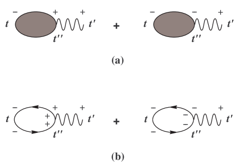
Figure 6.1: The Feynman diagrams that contribute to the invariant photon production rate from the QGP. Figure (a) shows the contribution to order $\alpha$ and to all orders in $\alpha_{s}$ with the blob denoting the full quark electromagnetic current correlation function to all orders in $\alpha_{s}$. Figure (b) is the lowest order contribution, of order $\alpha$.

We focus here on the lowest order (one-loop) contribution, which is missed by all the previous investigations using the $S$-matrix approach implicitly assuming an infinite QGP lifetime. To lowest order in perturbation theory, neglecting the vacuum contribution one obtains the invariant photon production rate for a QGP of two light quark flavors ($u$ and $d$) to be given by

$$E\frac{dN(t)}{d^{3}p\,d^{4}x} = \frac{2}{(2\pi)^{3}}\int_{t_{i}}^{t}dt^{\prime\prime}\int_{-\infty}^{+\infty}\frac{d\omega}{\pi}\,\mathcal{R}(\omega)\,\cos[(\omega-E)(t-t^{\prime\prime})],$$ (6.17)

where

$$\mathcal{R}(\omega) = \frac{20\,\pi^{2}\alpha}{3}\int\frac{d^{3}q}{(2\pi)^{3}}\Big{[}2\big{[}1-(\mathbf{\hat{p}}\cdot\mathbf{\hat{k}})(\mathbf{\hat{p}}\cdot\mathbf{\hat{q}})\big{]}n(q)[1-n(k)]\delta(\omega+k-q)$$ (6.18)

$$+\big{[}1+(\mathbf{\hat{p}}\cdot\mathbf{\hat{k}})(\mathbf{\hat{p}}\cdot\mathbf{\hat{q}})\big{]}n(q)n(k)\delta(\omega-k-q)\Big{]},$$

with $n(q)=1/[e^{q/T_{i}}+1]$ the quark distribution function at the initial time $t_{i}$. We note that in obtaining the above expressions, we have used the free quark propagators which correspond to hard quark loop momentum ($q\gtrsim T_{i}$). Soft quark lines ($q\ll T_{i}$) require using the HTL-resummed effective quark propagator [62], thereby leading to higher order corrections. Indeed, the one-loop diagram with soft quark loop momentum is part of the higher order contribution of order $\alpha\alpha_{s}$ that has been calculated in Refs. [112, 113].

We note that apart from color and flavor factors $\mathcal{R}(\omega)$ given by Eq. (6.18) has the same structure as the first two terms in $\mathcal{R}^{<}_{\gamma}(\omega,k)$ given by Eq. (5.49). From the discussion there, one finds that the first delta function $\delta(\omega+k-q)$ has support below the light cone ($\omega^{2}<E^{2}$) corresponding to the Landau damping cut whereas the second delta function $\delta(\omega-k-q)$ has support above the light cone corresponding to the usual two-particle cut. Furthermore, $\mathcal{R}(\omega)$ has a clear physical interpretation in terms of the following energy-nonconserving photon production processes: the first term describes (anti)quark bremsstrahlung $q(\bar{q})\rightarrow q(\bar{q})\gamma$, and the second term describes quark-antiquark annihilation to photon $q\bar{q}\rightarrow\gamma$.

The dependence of $\mathcal{R}(\omega)$ on the quark distribution at the initial time $t_{i}$ is a consequence of the fact that in nonequilibrium quantum field theory the important ingredient is the initial density matrix, which consistent with hydrodynamics is taken to be thermal for quarks and gluons. Since the calculation is carried out consistently in perturbation theory, the quark (and gluon) propagators are in terms of the equilibrium free particle distribution functions. In the case of a nonexpanding and thermalized QGP, the integral over $t^{\prime\prime}$ in Eq. (6.17) can be carried out directly leading to

$$E\frac{dN(t)}{d^{3}p\,d^{4}x}=\frac{2}{(2\pi)^{3}}\int_{-\infty}^{+\infty}d\omega\,\mathcal{R}(\omega)\,\frac{\sin[(\omega-E)(t-t_{i})]}{\pi(\omega-E)},$$ (6.19)

At this stage we can make contact with the $S$-matrix calculation and highlight the importance of the finite-time, nonequilibrium analysis. If, as is implicit in the $S$-matrix calculation, the QGP is assumed in thermal equilibrium and with an infinite lifetime (entailing that $t_{i}\rightarrow-\infty$ and $t_{f}\rightarrow\infty$), then we can take the infinite time limit $t_{i}\rightarrow-\infty$ in the argument of the sine function in Eq. (6.19) and use the approximation

$$\frac{\sin[(\omega-E)t]}{\pi(\omega-E)}\buildrel t\rightarrow\infty\over{\approx}\delta(\omega-E).$$ (6.20)

This is the assumption of completed collisions that is invoked in time-dependent perturbation theory leading to Fermi’s golden rule and energy conservation. The delta function $\delta(\omega-E)$ is a manifestation of energy conservation for each completed collision. Under this assumption one finds a time-independent photon production rate proportional to $\mathcal{R}(E)$, provided that the latter is finite. In the present situation, however, the delta functions in $\mathcal{R}(\omega)$ cannot be satisfied on the photon mass shell. Therefore, under the assumption of completed collisions the lowest order energy-nonconserving contribution to the photon production rate simply vanishes due to kinematics. Therefore this lowest order contribution is absent (by energy conservation) in the $S$-matrix calculation, but is present at any finite time.

The relevant question to ask is that how this finite-time contribution of order $\alpha$ compares to the higher order $S$-matrix contribution to the photon yield.

For finite QGP lifetime the time-dependent rate given in Eq. (6.19) is finite and nonvanishing, thus leading to a nontrivial contribution to direct photon production. The photon yield (per unit volume) is obtained by integrating the rate over the lifetime of the QGP. Using Eq. (6.19), one obtains

$$E\frac{dN}{d^{3}p~{}d^{3}x}=\frac{2}{(2\pi)^{3}}\int_{-\infty}^{+\infty}d\omega\,\mathcal{R}(\omega)\,\frac{1-\cos[(\omega-E)(t_{f}-t_{i})]}{\pi(\omega-E)^{2}},$$ (6.21)

where $t_{f}-t_{i}\sim 10\,{\rm fm}/c$ is the lifetime of the QGP.

Before proceeding further, we give an analytic estimate of the behavior of the photon yield in the HTL approximation. In this approximation the leading contribution of $\mathcal{R}(\omega)$ is dominated by the Landau damping cut, which corresponds to off-shell (anti)quark bremsstrahlung, and is found to be given by

$${\cal R}_{\mathrm{HTL}}(\omega)=\frac{20}{3}\frac{\pi^{2}\alpha T^{2}}{12}\frac{\omega}{E}\left(1-\frac{\omega^{2}}{E^{2}}\right)n_{B}(\omega)\,\theta(E^{2}-\omega^{2}),$$ (6.22)

where use has been made of the KMS condition, valid for quarks in thermal equilibrium.

For $E\ll T$, ${\cal R}_{\mathrm{HTL}}(\omega)$ can be further simplified as [see Eq. (5.51)]

$${\cal R}_{\rm HTL}(\omega)\buildrel E\ll T\over{\simeq}\frac{20}{3}\frac{\pi^{2}\alpha T^{3}}{12E}\left(1-\frac{\omega^{2}}{E^{2}}\right)\theta(E^{2}-\omega^{2}).$$ (6.23)

The dominant contribution of the $\omega$ integral in Eq. (6.21) for $E\ll T$ arises from the region where the resonant denominator vanishes ($\omega\approx E$). Using Eq. (6.23), we obtain

$$E\frac{dN(t)}{d^{3}p\,d^{3}x}\buildrel E\ll T\over{=}\frac{5}{9}\frac{\alpha}{2\pi^{2}}\frac{T^{3}}{E^{2}}\left[\ln 2Et+\gamma-1\right]+{\cal O}\left(\frac{1}{t}\right),$$ (6.24)

where $\gamma=0.577\ldots$ is the Euler-Mascheroni constant. Figure 6.2 displays the ratio of the hard ($E\sim T$) photon yield extrapolated from Eq. (6.24) and that obtained from the equilibrium rate of Kapusta et al. given by Eq. (6.9). We see clearly that the lowest order $\mathcal{O}(\alpha)$ nonequilibrium contribution to the photon yield is comparable at early times to the higher order $\mathcal{O}(\alpha\alpha_{s})$ equilibrium contribution.

Figure 6.2: The ratio of the nonequilibrium and equilibrium hard ($E\sim T$) photon yield plotted as a function of time for $\alpha=1/137$, $\alpha_{s}=0.3$ and $T=200$ MeV (see text for details).

For $E\gg T$, as depicted in Fig. 6.3, ${\cal R}_{\mathrm{HTL}}(\omega)$ is exponentially suppressed in the region $T<\omega<E$. From this observation we emphasize the following important features of the nonequilibrium yield given by Eq. (6.21). (i) Because for $E\gg T$ the threshold contribution near the photon mass shell $\omega\approx E$ is exponentially suppressed, the $\omega$ integral in Eq. (6.21) is now dominated by the interval $-E<\omega<T$, which corresponds to highly off-shell (anti)quark bremsstrahlung. (ii) As the integrand in Eq. (6.21) is positive-definite and the function $1-\cos[(\omega-E)t]$ averages to 1 for large $t$ in the region $-E<\omega<T$, for fixed $E\gg T$ the yield approaches a constant at large times. (iii) In contrast to those obtained from equilibrium rates, the yield for $E\gg T$ is not suppressed by the Boltzmann factor $e^{-E/T}$.

Figure 6.3: The function ${\cal R}_{\rm HTL}(\omega)$ plotted in the limit $E\gg T$. Here we take $E=2$ GeV and $T=200$ MeV.

Figure 6.4 shows a comparison of the nonequilibrium and equilibrium contributions to the hard photon yield in the range of energy $T<E<5$ GeV from a QGP of temperature $T=200$ MeV and lifetime $t=10$ fm/$c$. Whereas the two-loop contribution dominates the direct photon yield for smaller values of $E$, a significant enhancement of the direct photon yield due to the nonequilibrium contribution is seen at $E>2$ GeV as a consequence of its power law falloff for $E\gg T$. Numerical evidence shows that the nonequilibrium yield $EdN(t)/d^{3}p\,d^{3}x$ falls off with a power law $E^{-\nu}$ with $\nu\approx 2.14$ for $T\ll E<5$ GeV. In particular, the nonequilibrium contribution is larger than the equilibrium contributions by several orders of magnitude for $E>3$ GeV. As the nonequilibrium contribution for fixed $E\gg T$ approaches a constant at large times, the equilibrium contributions, which grow linearly in time, will eventually dominate the yield if the QGP has a very long lifetime. However, the linear growth in time of the equilibrium contributions has to compensate the Boltzmann suppression for $E\gg T$. Therefore we emphasize that for $E\gg T$ the equilibrium contributions could dominate the yield only if the QGP lifetime is of order $10^{2}-10^{3}$ fm/$c$ or larger, which nevertheless is very unrealistic at RHIC energies.

Figure 6.4: Comparison of various contributions to the direct photon yield from a QGP of temperature $T=200$ MeV and lifetime $t=10$ fm/$c$. The inset shows the figure on a log-log plot.

While these results in the nonexpanding case revealed the importance of the nonequilibrium and finite-lifetime aspects, the most experimentally relevant case to study is that of an expanding QGP. This experimentally relevant case can only be investigated by a detailed numerical study.

6.4.2 Longitudinally expanding QGP

As a prelude to photon production from an expanding QGP, we first focus on the invariant photon production rate from each individual fluid cell of the QGP. Since the proper time equals to the local time in the local rest frame of any fluid cell, we can follow the same real-time nonequilibrium analysis presented in the proceeding subsection to calculate the nonequilibrium invariant photon production rate in the local rest frame of each fluid cell. We obtain

$$E\frac{dN(\tau)}{d^{3}p\,d^{4}x}\bigg{|}_{\rm LR}=\lim_{\tau^{\prime}\rightarrow\tau}\frac{\partial}{\partial\tau^{\prime}}\sum^{N_{f}}_{f=1}\frac{e\,e_{f}}{2(2\pi)^{3}}\int\frac{d^{3}q}{(2\pi)^{3}}\big{\langle}\bar{\psi}_{f}^{-}(-{\bf k},\tau){\boldsymbol{\gamma}}\cdot{\bf A}^{+}_{T}({\bf p},\tau^{\prime})\psi_{f}^{-}({\bf q},\tau)\big{\rangle}+\mbox{c.c.}.$$ (6.25)

As before, the nonequilibrium expectation values on the right-hand side of Eq. (6.25) is computed perturbatively to order $\alpha$ and in principle to all orders in $\alpha_{s}$ by using real-time Feynman rules and propagators. To lowest order in perturbation theory, the result for two light quark flavors ($u$ and $d$) reads

$$E\frac{dN(\tau)}{d^{3}p\,d^{4}x}\bigg{|}_{\rm LR}=\frac{2}{(2\pi)^{3}}\int_{\tau_{i}}^{\tau}d\tau^{\prime\prime}\int_{-\infty}^{+\infty}\frac{d\omega}{\pi}\,\mathcal{R}(\omega)\,\cos[(\omega-E)(\tau-\tau^{\prime\prime})],$$ (6.26)

where $\mathcal{R}(\omega)$ is the same as that given in Eq. (6.18), but now with $n(q)=1/[e^{q/T_{i}}+1]$ being the quark distribution function at initial proper time $\tau_{i}$, at which the QGP reaches local thermal equilibrium.

In principle in the case of an expanding QGP under consideration, the photon production rate given by Eq. (6.26) has to be supplemented by kinetic equations that describe the evolution of the quark and gluon distribution functions so as to setup a closed set of coupled equations. However the assumption of the validity of (ideal) hydrodynamics entails that the quarks and gluons form a perfectly coupled fluid. This in turn implies that the mean free paths of the quarks and gluons are much shorter than the typical wavelengths and the relaxation time scales are much shorter than the typical time scales, i.e., the quark and gluon distribution functions adjust to local thermal equilibrium instantaneously. Thus the assumption of the validity of (ideal) hydrodynamics bypasses the necessity of the coupled kinetic equations: quarks and gluons are in local thermal equilibrium at all times. Therefore, within the framework of hydrodynamics we obtain the invariant photon production rate by directly replacing the initial quark distribution function $n(q)$ in Eq. (6.18) by the “updated” distribution function $n[q,T(\tau^{\prime\prime})]=1/[e^{q/T(\tau^{\prime\prime})}+1]$ at proper time $\tau^{\prime\prime}>\tau_{i}$, where $T(\tau^{\prime\prime})$ is determined by the cooling law Eq. (6.12). The nonequilibrium invariant photon production rate that is consistent with the underlying hydrodynamics is then given by

$$E\frac{dN}{d^{3}p\,d^{4}x}\bigg{|}_{\rm LR}[\tau,E,T(\tau)]=\frac{2}{(2\pi)^{3}}\int_{\tau_{i}}^{\tau}d\tau^{\prime\prime}\int_{-\infty}^{+\infty}\frac{d\omega}{\pi}\,\mathcal{R}[\omega,T(\tau^{\prime\prime})]\,\cos[(\omega-E)(\tau-\tau^{\prime\prime})],$$ (6.27)

with

$$\mathcal{R}[\omega,T(\tau)] = \frac{20\,\pi^{2}\alpha}{3}\int\frac{d^{3}q}{(2\pi)^{3}}\Big{[}2\big{[}1-({\bf\hat{p}}\cdot{\bf\hat{k}})({\bf\hat{p}}\cdot{\bf\hat{q}})\big{]}n[q,T(\tau)]\bar{n}[k,T(\tau)]\delta(\omega+k-q)$$ (6.28)

$$+\,\big{[}1+({\bf\hat{p}}\cdot{\bf\hat{k}})({\bf\hat{p}}\cdot{\bf\hat{q}})\big{]}n[q,T(\tau)]n[k,T(\tau)]\delta(\omega-k-q)\Big{]},$$

where $n[q,T(\tau)]=1/[e^{q/T(\tau)}+1]$ and $\bar{n}=1-n$. The momentum $q$ integrals in Eq. (6.28) are calculated in the LR frame and hence are equivalent to those of the nonexpanding case above.

Before proceeding further, we emphasize two noteworthy features of the nonequilibrium invariant photon production rate: (i) The photon production processes do not conserve energy. (ii) The rate depends on (proper) time not only implicitly through the local temperature but also explicitly. Furthermore, this explicit (proper) time dependence is non-Markovian as clearly displayed in Eq. (6.27). Whereas these two features seem rather uncommon in transport phenomena in heavy ion collisions (see, however, Refs. [72, 128]), they are not unusual in nonrelativistic many-body quantum kinetics under extreme conditions [29]. In particular, energy-nonconserving transitions and memory effects which cannot be explained by usual (semiclassical) Boltzmann kinetics have been observed recently in ultrafast spectroscopy of semiconductors with femtosecond laser pulses [32].

The real-time kinetic approach when incorporated consistently with the hydrodynamical evolution of the QGP reveals clearly that photon production is inherently a nonequilibrium quantum effect associated with the expansion and finite lifetime of the QGP.

At RHIC and LHC energies the quark distribution function $n[q,T(\tau)]$ depends on the proper time $\tau$ very weakly through the temperature $T(\tau)$ within the lifetime of the QGP phase, hence a Markovian approximation (MA) in which the temperature in $\mathcal{R}[\omega,T(\tau^{\prime\prime})]$ is taken at the upper limit of the integral is reasonable and hence the memory kernel may be simplified. In this Markovian approximation, $\mathcal{R}[\omega,T(\tau^{\prime\prime})]$ in Eq. (6.27) is replaced by $\mathcal{R}[\omega,T(\tau)]$ and taken outside of the $\tau^{\prime\prime}$-integral. Thus Eq. (6.27) becomes

$$E\frac{dN}{d^{3}p\,d^{4}x}\bigg{|}^{\rm MA}_{\rm LR}[\tau,E,T(\tau)]=\frac{2}{(2\pi)^{3}}\int_{-\infty}^{+\infty}d\omega\,\mathcal{R}[\omega,T(\tau)]\,\frac{\sin[(\omega-E)(\tau-\tau_{i})]}{\pi(\omega-E)}.$$ (6.29)

A computational advantage of this Markovian nonequilibrium production rate is that it provides the “updated” quark distribution functions locally in time. Physically, the motivation for this approximation is that the most important aspect of the nonequilibrium effect is the nonconservation of energy originated in the finite lifetime of the QGP, a feature that is missed by the usual $S$-matrix calculation, while the proper time variation of the temperature is a secondary effect and accounted for in the $S$-matrix approach.

It is worth noting that a connection with the Boltzmann approximation can be obtained by assuming completed collisions, i.e., taking the limit $\tau_{i}\rightarrow-\infty$ in the argument of the sine function in Eq. (6.29) and using the approximation given by Eq. (6.20). Consequently, the lowest order nonequilibrium photon production rate vanishes in the Boltzmann approximation due to kinematics. This highlights, once again, that the usual approach to photon production outlined in Sec. 6.2 and used in the literature corresponds to the Boltzmann approximation and therefore fails to capture the energy-nonconserving and memory effects that occur during the transient stage of evolution of the QGP.

We are now in a position to calculate the direct photon yield from a longitudinally expanding QGP. In the CM frame the invariant production rate for photons of four-momentum $P^{\mu}$ from a fluid cell with four-velocity $u^{\mu}$ can be obtained from Eq. (6.29) through the replacement $E\rightarrow P^{\mu}u_{\mu}$. In terms of the photon transverse momentum $p_{T}$ and rapidity $y$, one finds $P^{\mu}u_{\mu}=p_{T}\cosh(y-\eta)$. The photon yield is obtained by integrating the nonequilibrium rate over the space-time evolution of the expanding QGP. Assuming a central collision of identical nuclei, in the Markovian approximation we find the invariant nonequilibrium photon yield to lowest order in perturbation theory to be given by

$$\frac{dN}{d^{2}p_{T}\,dy}\bigg{|}^{\rm MA}_{\rm CM}=\pi R_{A}^{2}\int_{\tau_{i}}^{\tau_{f}}d\tau\,\tau\int_{-\eta_{\rm cen}}^{\eta_{\rm cen}}d\eta\,E\frac{dN}{d^{3}p\,d^{4}x}\bigg{|}^{\rm MA}_{\rm LR}[\tau,P^{\mu}u_{\mu},T(\tau)],$$ (6.30)

where $R_{A}$ is the radius of the nuclei and $-\eta_{\rm cen}<\eta<\eta_{\rm cen}$ denotes the central rapidity region within which Bjorken’s hydrodynamical model is valid.

As remarked above, at RHIC and LHC energies the quark distribution function $n[q,T(\tau)]$ depends on the proper time $\tau$ very weakly through the temperature $T(\tau)$ within the lifetime of the QGP phase, therefore the resultant photon yield is expected to qualitatively resemble the nonequilibrium photon yield from a nonexpanding QGP studied in above. This will be numerically verified below. We note that the expanding and nonexpanding cases differ mainly by the Jacobian $\tau$ in the $\tau$ integral in Eq. (6.30) that accounts for the longitudinal expansion of the QGP, and by the replacement $E\rightarrow P^{\mu}u_{\mu}$ in the argument of the invariant photon production rate that accounts for the shift of the photon energy under local Lorentz boost .

6.4.3 Numerical analysis: central collisions at RHIC and LHC energies

We now perform a numerical analysis of the nonequilibrium photon yield and compare the results to the equilibrium one obtained from higher order equilibrium rate calculations given by Eqs. (6.9) and (6.10). The nonequilibrium photon yield in the Markovian approximation given by Eq. (6.30) contains a four-dimensional integral that is performed numerically for the values of parameters of relevance at RHIC and LHC energies.

Figure 6.5: Comparison of nonequilibrium (solid) and equilibrium (dotted) photon yields at midrapidity ($y=0$) from a longitudinally expanding QGP at RHIC energies with initial conditions given by $\tau_{i}=1$ fm/$c$ and $T_{i}=200$ (top), 300 (bottom) MeV.

For central ¹⁹⁷Au$+{}^{197}$Au collisions at RHIC energies $\sqrt{s_{NN}}\sim 200$ GeV, we take $R_{A}\simeq 1.2\,A^{1/3}$ fm $\approx 7$ fm [43] and $\eta_{\rm cen}=2$. The initial thermalization time is taken to be $\tau_{i}=1$ fm/$c$ [123, 124], the final proper time $\tau_{f}$ is determined when the critical temperature for the quark-hadron transition is reached at $T(\tau_{f})\simeq 160$ MeV and is obtained from the cooling law given by Eq. (6.12) for a given initial temperature $T_{i}$ at proper time $\tau_{i}$.

The nonequilibrium photon yield at midrapidity ($y=0$) in the range of transverse momentum $0.3<p_{T}<5$ GeV/$c$ is shown on a log-log plot in Fig. 6.5 for initial temperatures $T_{i}=200$ and 300 MeV. For comparison we also plot the corresponding equilibrium yield obtained by integrating Eqs. (6.9) and (6.10) with the transformation to the CM frame as specified by Eq. (6.14), and using the value of $\alpha_{s}$ [122, 123, 129]

$$\alpha_{s}[T(\tau)]=\frac{6\pi}{(33-2N_{f})\ln[8\,T(\tau)/T_{c}]},$$ (6.31)

with $N_{f}=2$. Furthermore, Fig. 6.6 shows the rapidity distribution of the nonequilibrium photon yield at different values of $p_{T}$ for $T_{i}=200$ and $300$ MeV. Several noteworthy features are gleaned from these figures:

Figure 6.6: Rapidity distribution of the nonequilibrium photon yield at $p_{T}=1$ (solid), 2 (dotted), and 3 (dashed) GeV for a longitudinal expanding QGP at RHIC energies with initial conditions given by $\tau_{i}=1\,{\rm fm}/c$ and $T_{i}=200$ (top), 300 (bottom) MeV. The distribution is symmetric at $y=0$.

1. Whereas the equilibrium yield dominates the total yield for small $p_{T}$, the nonequilibrium yield becomes significantly dominant in the range $p_{T}>1.0-1.5$ GeV/$c$. Perhaps coincidentally, this is the range in which the CERN WA98 data for central Pb$+$Pb collisions at SPS energies shows a distinct excess [119].

2. While the equilibrium yield leads to a transverse momentum distribution that falls off approximately with the Boltzmann factor $e^{-p_{T}/T_{i}}$, the nonequilibrium yield is not Boltzmann suppressed and falls off algebraically. It is found numerically that for $p_{T}\gg T_{i}$ and within the region $1\lesssim p_{T}\lesssim 5$ GeV/$c$ the nonequilibrium yield at midrapidity falls off with a power law $p_{T}^{-\nu}$ with $\nu\simeq 2.47$ and $2.77$ for $T_{i}=200$ and 300 MeV, respectively. This is a remarkable consequence of the fact that bremsstrahlung is the dominant process. As discussed in detail above at large energies the dominant process is bremsstrahlung corresponding to the contribution from the term $n(q)[1-n(k)]$ with $k=|\mathbf{p}+\mathbf{q}|$ in Eq. (6.18). For large photon energy $p$ the important contribution, which is not exponentially suppressed arises from the small $q$ region.

3. A central plateau in the range of rapidity $y\lesssim 2$ is seen clearly. The rapidity distribution begins to bend down when $y\simeq\eta_{\rm cen}$, i.e., when the photon rapidity probes the fragmentation region.

4. The numerical analysis of the expanding case reveals features very similar to those found in the nonexpanding case, where we estimate that for $p_{T}\geq 1.5$ GeV/$c$ the higher order equilibrium contribution to the direct photon yield (which grows linearly in time) becomes of the same order as the lowest order nonequilibrium contribution (which grows at most logarithmically in time) only if the lifetime of the QGP is of the order longer than 1000 fm/$c$. Therefore, we conclude that these nonequilibrium effects dominate during the lifetime of the QGP in a realistic ultrarelativistic heavy ion collision experiment.

Figure 6.7: Comparison of nonequilibrium (solid) and equilibrium (dotted) photon yields at midrapidity ($y=0$) from a longitudinally expanding QGP at LHC energies with initial conditions given by $\tau_{i}=1$ fm/$c$ and $T_{i}=450$ (top), 500 (bottom) MeV.

Similar numerical analysis can be performed for central ²⁰⁸Pb$+{}^{208}$Pb collisions at higher LHC energies $\sqrt{s_{NN}}\sim 5500$ GeV, for which we take $R_{A}\approx 7$ fm, $\eta_{\rm cen}=5$ and $\tau_{i}=1$ fm/$c$ [123, 124]. The comparison of nonequilibrium and equilibrium photon yields at midrapidity is displayed in Fig. 6.7 for $T_{i}=450$ and 500 MeV. The dominance of the nonequilibrium yield at high $p_{T}$ remains but now at higher transverse momentum $p_{T}\gtrsim 2$ GeV. This can be understood as a consequence of the longer QGP lifetime resulting from higher initial temperature at LHC energies. Furthermore, it is found numerically that for $1\lesssim p_{T}\lesssim 5$ GeV/$c$ the nonequilibrium yield at midrapidity falls off with a power law $p_{T}^{-\nu}$ with $\nu\simeq 2.52$ and $2.56$ for $T_{i}=450$ and 500 MeV, respectively.

These results indicate a clear manifestation of the nonequilibrium aspects of direct photon production associated with a transient QGP of finite lifetime. The most experimentally accessible signal of the nonequilibrium effects revealed by this analysis is the power law falloff of the transverse momentum distribution for direct photons in the range $1\lesssim p_{T}\lesssim$ 5 GeV/$c$ with an exponent $2.5\lesssim\nu\lesssim 3$ for temperatures expected at RHIC and LHC energies. Our numerical studies reveal that this exponent increases with initial temperature and therefore with the initial energy density of the QGP and the total multiplicity rapidity distribution $dN_{\pi}/dy$ [124]. This could be a clean experimental nonequilibrium signature of a transient QGP since the photon distribution from the hadronic gas is expected to feature a Boltzmann type exponential suppression for $p_{T}\gg T_{i}$ [112, 121, 122, 123].

6.5 Conclusions

In this chapter we study an important phenomenological application of the real-time quantum kinetic techniques developed in previous chapters. Our goal is to search for clear experimental signatures of direct photon production associated with nonequilibrium aspects of the transient QGP created in ultrarelativistic heavy ion collisions at RHIC and LHC energies.

We first argue that the usual $S$-matrix approach to direct photon production from an expanding nonequilibrium QGP has conceptual limitations. Instead we introduce a real-time kinetic approach that allows a consistent treatment of photon production from a transient nonequilibrium state of finite lifetime.

We focus on obtaining the direct photon yield from a thermalized QGP undergoing Bjorken’s hydrodynamical expansion in central Au$+$Au collisions at RHIC ($\sqrt{s_{NN}}\sim 200$ GeV) and LHC ($\sqrt{s_{NN}}\sim 5500$ GeV) energies. The lifetime of a QGP for these collisions is of order $10-30$ fm/$c$. We find that energy-nonconserving (anti)quark bremsstrahlung $q(\bar{q})\rightarrow q(\bar{q})\gamma$ and quark-antiquark annihilation $q\bar{q}\rightarrow\gamma$, both of lowest order in $\alpha$, dominate during such short time scales with bremsstrahlung dominating for $p_{T}\gg T_{i}$. The contribution from these processes is a consequence of the transient nature and the finite lifetime of the QGP. As compared to the equilibrium rate calculations, the energy-nonconserving processes lead to a substantial enhancement in direct photon production for $1-2\lesssim p_{T}\lesssim 5$ GeV/$c$ near midrapidity. In striking contrast with the equilibrium calculation that predicts an exponential suppression of the transverse momentum distribution for $p_{T}\gg T_{i}$ ($T_{i}$ is the initial temperature), the nonequilibrium processes lead to a power law behavior instead. We find that at RHIC and LHC energies the direct photon transverse momentum distribution near midrapidity is of the form $p^{-\nu}_{T}$ with $2.5\lesssim\nu\lesssim 3$ for $1\lesssim p_{T}\lesssim 5$ GeV/$c$ and that photon rapidity distribution (for fixed $p_{T}$) is almost flat in the interval $|y|\lesssim\eta_{\rm cen}$, where $|\eta|<\eta_{\rm cen}$ denotes the central rapidity region of the QGP. The exponent $\nu$ is numerically found to increase with the initial temperature, hence increases with the total multiplicity rapidity distribution $dN_{\pi}/dy$, which is an experimental observable.

Thus, as the main conclusion, we propose that direct photons are distinct experimental signatures of the transient nonequilibrium QGP created at RHIC and LHC energies, both in the form of a large enhancement at $1-2\lesssim p_{T}\lesssim$ 5 GeV/$c$ as well as a power law transverse momentum distribution $p^{-\nu}_{T}$ with an exponent $\nu$ that is within the range $2.5\lesssim\nu\lesssim 3$ and increases with total multiplicity rapidity distribution $dN_{\pi}/dy$.

Our study of direct photon production focuses solely on the QGP phase and neglects contributions from pre-equilibrium stage as well as the mixed and hadronic phases, because we focus on a comparison between the usual equilibrium approach and the kinetic real-time approach that allows for following the time evolution of the density matrix as an initial value problem consistent with hydrodynamics. Furthermore, as discussed elsewhere in the literature, since most of the high-$p_{T}$ photons originate from the very early, hot stage in the QGP phase [110, 112, 114] and photons produced in the mixed phase as well as the subsequent hadronic phase are mainly in the lower-$p_{T}$ region [123], the nonequilibrium yield from the QGP phase contributes dominantly to the total high-$p_{T}$ photons.

We have provided a systematic real-time description compatible with the initial value problem associated with hydrodynamic evolution, however more needs to be understood for a complete description of all the different stages. The parton cascade approach to describe the early pre-equilibrium stage after the collision is an important first step in a full microscopic description, but perhaps a more consistent description of the initial condition for QGP formation must be based on the recent notions of a color glass condensate [131, 132]. Hence, a complete treatment of the direct photon yield must, in principle, begin from the initial stage, possibly a color glass condensate, and obtain the real-time evolution of photon production. Clearly there must be many more advances in this field before such a program becomes feasible. The finite-temperature equilibrium calculations assume that the equilibrium thermal state always prevailed, thus ignores completely not only the initial stages but also the time evolution. Our approach while incorporating the time evolution consistently, also neglects the initial stage. We have focused on direct photons from a transient QGP for a direct comparison with equilibrium calculations, but obviously photons will continue to be produced during the mixed and hadronic phases. A detailed understanding of the transition as well as the hadronic photon production matrix elements is necessary for a more reliable estimate of the potential nonequilibrium effects after hadronization.

Although we do not claim to have provided a completely detailed understanding of potential nonequilibrium effects due to the lack of knowledge of initial conditions in heavy ion collisions, we do claim that our approach provides a more systematic description of the finite-lifetime effects associated with a transient QGP. These effects lead to a distinct experimental prediction: a power law falloff of the distribution $dN/d^{2}p_{T}dy$ near the central rapidity region which is distinguishable from a thermal tail for $1-2\lesssim p_{T}\lesssim 5$ GeV/$c$. We note that the parton-cascade results of photon production from the pre-equilibrium stage [126] also seem to reveal a power law falloff of the photon distribution in this range of transverse momentum with comparable order of magnitude and exponent, as can be gleaned from Figs. 2 and 3 of Ref. [126]. Perhaps these two effects, namely the prompt photons from the pre-equilibrium stage and the direct photons from the hydrodynamically expanding QGP with a finite lifetime cannot be distinguished experimentally. Nevertheless, we emphasize that a power law departure from a thermal tail in the direct photon spectrum may very well be explained by nonequilibrium effects, either by a finite QGP lifetime as advocated in this chapter or by prompt photons from the pre-equilibrium stage.

An important and very relevant question is that why not treat high energy particle collisions in the same manner, i.e., with the real-time evolution rather than with the $S$-matrix approach. The answer to this question hinges on the issue of time scales. In a typical high energy particle collider experiment, the colliding “beams” are actually bunches or packets with a typical spatial extent of order $1-10$ cm and hence the typical time interval for the collision is of order $10^{-9}$ sec. This time scale is many orders of magnitude longer than the typical hadronic interaction time scale $\sim 10^{-23}$ sec, thus taking the infinite time limit is amply justified. This of course is the basis for using the $S$-matrix calculation in terms of asymptotic in and out states (at $t=\mp\infty$): the total interaction time is much, much longer than the typical hadronic time scale. With regard to the heavy ion collision, the consensus is that after an initial pre-equilibrium stage, a locally thermalized QGP is formed. It then evolves hydrodynamically, hadronizes and eventually the freeze-out of hadronic gas ensues. Current theoretical estimates indicate a total time between formation and freeze-out of order $50-100$ fm/$c$, with a QGP phase lasting for about $10$ fm/$c$. These time scales are not several orders of magnitude larger than the hadronic interaction time scale, thus the infinite time limit taken in the $S$-matrix calculation is at best questionable. Therefore while in typical particle collider experiments the $S$-matrix approach is valid (as has been demonstrated by half a century of experiments), the transient QGP with a finite lifetime of the order of the hadronic time scales merits a different treatment.

As many recent investigations [130] have suggested that the QGP produced at RHIC and LHC energies is not expected to be in local chemical equilibrium, i.e., the distribution functions of quarks and gluons will probably be undersaturated, an important extension of our work will be the study of nonequilibrium effects on direct photon production from a chemically nonequilibrated QGP. Another important aspect that requires further investigation is the finite size of the QGP. Much in the same way as the finite lifetime introduces nonequilibrium effects associated with energy nonconserving transitions, we expect that the finite size $\sim 7$ fm of the QGP will introduce uncertainty in the momentum of the emitted particles. This is clearly an important topic that deserves further and deeper study but is beyond the scope of this thesis. However, at this stage we speculate that if such effects are present they could bear an imprint in transverse flow [65].

Chapter 7 Summary

The central theme of this thesis is the study of real-time nonequilibrium quantum dynamics with specific focus on the real-time relaxation of the mean fields and quantum kinetics in a variety of physically relevant quantum field theories with applications to cosmology and ultrarelativistic heavy ion collisions. This study could be generalized to nonequilibrium problems in condensed matter physics, quantum optics and atomic physics. To conclude this thesis, we summarize our work and highlight the main results.

Fermion damping in a fermion-scalar plasma. We study the real-time relaxation of the fermion mean field in a fermion-scalar plasma which is relevant to models of baryogenesis at the electroweak scale. We begin by obtaining directly in real time the effective in-medium Dirac equation for the fermion mean field induced by an adiabatically switched-on external source. The in-medium Dirac equation is fully renormalized, retarded and causal, thereby leading to an initial value problem for the fermion relaxation.

For the light scalar which cannot decay into fermion pairs, we find that to lowest order in the Yukawa coupling the only medium effect on fermions is dispersive and in-medium propagation of fermion excitations is undamped. On the other hand, for the heavy scalar such that its decay into fermion pairs is kinematically allowed, we find a novel dissipative medium effect arises from scalar decay in the medium and leads to damping of fermion excitations. That is, the fermions acquire a width due to the decay of the heavy scalar in the medium and become quasiparticles with a finite lifetime. Solving the effective Dirac equation by Laplace transform, we obtained the time evolution of the fermion mean field which allows a clear identification of the damping rate. We calculate the damping rate in the narrow width approximation to one loop order for arbitrary values of the fermion and scalar masses (provided the scalar is heavy enough to decay), temperature and fermion momentum. An all-order expression for the damping rate in terms of the exact quasiparticle wave functions is established by analyzing the structure of the fermion self-energy.

Finally, a Boltzmann-type kinetic equation for the fermion distribution function in the relaxation time approximation confirms the damping of fermion excitations as a consequence of the decay of heavy scalars in the medium, and displays the relationship between the fermion damping rate and interaction rate to lowest order in the Yukawa coupling directly in real time.

Dynamical renormalization group approach to quantum kinetics. We provide an alternative first-principle derivation of quantum kinetic equations in quantum field theory by implementing a diagrammatic perturbative expansion improved by a resummation via the dynamical renormalization group directly in real time.

This method begins by obtaining the equation of motion for the quasiparticle distribution function in perturbation theory. The solution of this equation of motion at large times reveals secular terms that grow with time, as a consequence of the fact that the perturbative analysis breaks down at large times. We implement the dynamical renormalization group to resum these secular terms directly in real time, the corresponding dynamical renormalization group equation, which describes the time evolution of the quasiparticle distribution function insensitive to the physics on microscopic time scales, is interpreted as the quantum kinetic equation. A remarkable feature of this method is that it allows to include consistently medium effects via resummation akin to the hard thermal loops but away from equilibrium.

We establish a close relationship between the dynamical renormalization group approach and the renormalization group in Euclidean field theory. In particular, coarse graining, stationary solutions, relaxation time approximation and relaxation rates have a natural parallel as irrelevant operators, fixed points, linearization near the fixed point and stability exponents, respectively, in the usual Euclidean renormalization group. This identification brings a new and rather different perspective to kinetics and relaxation that will hopefully lead to a new insights.

We then apply this novel method to study quantum kinetics of pions and sigma mesons in the $O(4)$ chiral linear sigma model. We derive the quantum kinetic equations that describes the time evolution of the pion and sigma meson distribution functions. The pion and sigma meson relaxation rates calculated in relaxation time approximation and agree with the corresponding damping rates found in the literature. We also find that in large momentum limit the emission and absorption of massless pions result in threshold infrared divergence in sigma meson relaxation rate and lead to a crossover behavior in relaxation that is unambiguously captured by the dynamical renormalization group analysis.

Furthermore by establishing a direct correspondence between pinch singularities and secular terms, we show that the dynamical renormalization group approach to quantum kinetics provides a natural framework to interpret and resolve the issue of pinch singularities in nonequilibrium quantum field theory.

Nonequilibrium dynamics in a QED plasma at high temperature. We study real-time nonequilibrium dynamics in a QED plasma at high temperature within the hard thermal loop (HTL) approximation by implementing the dynamical renormalization group. The goal is to understand the relaxation of photon and fermion mean fields directly in real time and quantum kinetics of the photon and fermion distribution functions beyond the usual Boltzmann description of kinetics. As many features of a hot QCD plasma are similar to those of a hot QED plasma, in addition to its direct impacts on astrophysics and cosmology, this study is also of phenomenological importance in ultrarelativistic heavy ion collisions. In particular, the leading contributions in the hard thermal loop approximation can be generalized easily from hot QED to hot QCD, thus relaxation of quarks and production of photons in the QGP can be understood to leading order from the study of a hot QED plasma.

For semihard photons of momentum $eT\ll k\ll T$, we find to leading order in the HTL approximation that the photon mean field relaxes with a power law $\sim t^{-e^{2}T^{2}/12k^{2}}$ at large times $t\gg 1/k$, as a result of infrared enhancement of the photon spectral density near the Landau damping threshold. The quantum kinetic equation for the distribution function of semihard photons, which includes off-shell effects missed by the usual Boltzmann description, is derived directly in real time from first principles in the relaxation time approximation by using the dynamical renormalization group method. We find that the distribution function also relaxes with a power law, with an exponent which is twice that for the photon mean field. The dynamical renormalization group analysis reveals the emergence of detailed balance on microscopic time scales larger than $1/k$ while the rates are still varying with time.

We show directly in real time that as a consequence of the emission and absorption of soft, quasi-static magnetic photons, hard fermion mean field with momentum $k\sim T$ exhibits a nonexponential relaxation at large times as $\sim e^{-\alpha Tt(\ln\omega_{P}t+0.126\ldots)}$, where $\omega_{P}=eT/3$ is the plasma frequency and $\alpha=e^{2}/4\pi$. A quantum kinetic equation for the distribution function of hard fermions in the relaxation time approximation is obtained directly in real time by implementing the dynamical renormalization group resummation. Unlike that of the usual Boltzmann kinetic equation derived in the quasiparticle approximation, the collision term of this quantum kinetic equation is time-dependent and infrared finite. The distribution function is found to relax nonexponentially with an anomalous exponent twice as large as that for the hard fermion mean field.

Our real-time analysis reveals clearly the limitation of the usual Boltzmann description of kinetics and the quasiparticle approximation in the study of nonequilibrium quantum dynamics in gauge field theory and has important impacts on direct photon production from the quark-gluon plasma.

Direct photon production from the quark-gluon plasma. As an important phenomenological application of real-time nonequilibrium dynamics in quantum field theory, we study direct photon production from a longitudinally expanding QGP at RHIC and LHC energies. Instead of focusing on obtaining an equilibrium photon production rate using the usual $S$-matrix formalism, we study photon production as an initial value problem with the real-time quantum kinetic description developed in this work.

This real-time approach allows us to incorporate consistently the kinetic description of photons with the hydrodynamical description of the QGP. Within Bjorken’s hydrodynamical model, we show that the lowest order energy-nonconserving (anti)quark bremsstrahlung $q(\bar{q})\rightarrow q(\bar{q})\gamma$ and quark-antiquark annihilation $q\bar{q}\rightarrow\gamma$ contribute dominantly to photon production during the transient lifetime of the QGP. For central collisions at RHIC ($\sqrt{s_{NN}}\sim 200$ GeV) and LHC ($\sqrt{s_{NN}}\sim 5500$ GeV) energies, we find a significant excess of direct photons in the range of transverse momentum $1-2\lesssim p_{T}\lesssim 5$ GeV/$c$ as compared to higher order equilibrium estimates. The rapidity distribution of photons is fairly flat near the midrapidity region. The remarkable result is that the transverse momentum distribution of photons at midrapidity falls off with a power law $p^{-\nu}_{T}$ with $2.5\lesssim\nu\lesssim 3$ as a consequence of the energy-nonconserving processes taking place during the transient lifetime of the QGP, providing a distinct nonequilibrium experimental signature of the QGP formation.

As summarized above, in this thesis we have advanced several aspects of real-time nonequilibrium dynamics in quantum field theory. In particular, we have established a theoretical framework for studying nonequilibrium dynamics of quantum multiparticle systems directly in real time from first principles. This framework is used to study a variety of physically relevant quantum field theories. It not only reproduces the usual results in the literature when the same approximations and assumptions are invoked, but also leads us to a new territory which has not been explored before. Most importantly, it is capable of making concrete predictions that can be tested experimentally at BNL RHIC and CERN LHC. We envisage our work will also have direct impacts on the understanding of nonequilibrium phenomena in condensed matter physics, quantum optics and cosmology.

Appendix A Renormalization Group and Asymptotic Analysis

In this appendix we present a pedagogical introduction to the renormalization group (RG) method in studying asymptotic analysis of ordinary differential equations. In order to introduce the basic idea, we consider a simple but illuminating example: a weakly damped harmonic oscillator. The reader is referred to Refs. [93, 94] for generalization to the much more complicated problems.

The differential equation governing a weakly damped harmonic oscillator is given by

$$\ddot{y}+y=-\epsilon\dot{y},\quad\epsilon\ll 1$$ (A.1)

with initial conditions $y(t_{0})$ and $\dot{y}(t_{0})$ specified at time $t_{0}$, where the overdot denotes the derivative with respect to $t$. Note that Eq. (A.1) can be solved exactly with the exact solution given by

$$y(t)=R_{0}\,e^{-\epsilon(t-t_{0})/2}\,\cos\left[\sqrt{1-\frac{\epsilon^{2}}{4}}\,(t-\Theta_{0})\right],$$ (A.2)

where $R_{0}$ and $\Theta_{0}$ are constants determined by the initial conditions. However, in order to demonstrate the renormalization group method, we attempt to solve Eq. (A.1) in a perturbative expansion in powers of $\epsilon$

$$y=y_{0}+\epsilon y_{1}+\epsilon^{2}y_{2}+\cdots.$$ (A.3)

Upon substituting the perturbative expansion into Eq. (A.1), one obtains a hierarchy of equations:

$$\ddot{y}_{0}+y_{0} = 0,$$

$$\ddot{y}_{1}+y_{1} = -\dot{y}_{0},$$ (A.4)

$$\ddot{y}_{2}+y_{2} = -\dot{y}_{1},$$

$$\vdots \vdots$$

Starting from the solution to the zeroth-order equation

$$y_{0}(t)=R_{0}\cos(t-\Theta_{0}),$$ (A.5)

and the zeroth-order retarded Green’s function

$$G_{0}^{R}(t-t^{\prime})=\sin(t-t^{\prime})\,\theta(t-t^{\prime}),$$ (A.6)

one obtains

$$y_{1}(t) = -\int^{t}_{t_{0}}dt^{\prime}\sin(t-t^{\prime})\,\dot{y}_{0}(t^{\prime})$$

$$= -\frac{R_{0}}{2}[(t-t_{0})\cos(t-\Theta_{0})-\cos(t_{0}-\Theta_{0})\sin(t-t_{0})],$$

$$y_{2}(t) = -\int^{t}_{t_{0}}dt^{\prime}\sin(t-t^{\prime})\,\dot{y}_{1}(t^{\prime})$$

$$= \frac{R_{0}}{8}\left[\left((t-t_{0})^{2}+\frac{1}{2}\right)\cos(t-\Theta_{0})-(t-t_{0})\sin(t-2t_{0}+\Theta_{0})-\cos(t-2t_{0}+\Theta_{0})\right].$$

Hence, to order $\mathcal{O}(\epsilon^{2})$ the solution is given by

$$y(t) = R_{0}\Biggl{\{}\left[1-\frac{\epsilon}{2}(t-t_{0})+\frac{\epsilon^{2}}{8}(t-t_{0})^{2}\right]\cos(t-\Theta_{0})-\frac{\epsilon^{2}}{8}(t-t_{0})\sin(t-2t_{0}+\Theta_{0})\Biggr{.}$$

$$+\,\Biggl{.}\frac{\epsilon}{2}\cos(t_{0}-\Theta_{0})\sin(t-t_{0})+\frac{\epsilon^{2}}{8}\left[\frac{1}{2}\cos(t-\Theta_{0})-\cos(t-2t_{0}+\Theta_{0})\right]\Biggr{\}}+\mathcal{O}(\epsilon^{3}).$$

It is noted that this solution contains secular terms that grow in $t$. This perturbative expansion breaks down for $\epsilon(t-t_{0})\gtrsim 1$ because of these secular terms. The presence of secular terms in a perturbative expansion indicates that perturbation method is only suitable to study short time behavior of a nonequilibrium system. To extract information of the long time behavior, one needs to go beyond the perturbation method. A close inspection of the secular terms in Eq. (LABEL:dosol) suggests the prefactor multiplying $\cos(t-\Theta_{0})$ resembles a time-dependent amplitude $R(t)$ and that multiplying $\sin(t-2t_{0}+\Theta_{0})$ resembles a time-dependent phase $\Theta(t)$.

The way to solve this difficulty of the perturbation method is to take account of its limitation and hence apply it only to describe short time behavior. The perturbative solution is evolved in time from $t_{0}$ only up to a time, say $t_{1}$, such that $\epsilon(t_{1}-t_{0})\ll 1$ and hence the perturbative solution is still reliable. Then the amplitude $R(t_{1})$ and phase $\Theta(t_{1})$ is used as the updated initial conditions at $t_{1}$ to iterate the perturbative solution forward in time to $t_{2}$ say $t_{1}$, such that $\epsilon(t_{2}-t_{1})\ll 1$. Repeating this procedure, one obtains an improved perturbative solution up to an arbitrary time $\tau$. The idea of renormalization group comes in when one wants to find out how the amplitude $R(\tau)$ and phase $\Theta(\tau)$ change as $\tau$ changes.

Let us assume that $R(\tau)$ and $\Theta(\tau)$ are related to $R_{0}$ and $\Theta_{0}$, respectively, by a multiplicative amplitude renormalization $Z_{R}(\tau)$ and an additive phase renormalization $Z_{\Theta}(\tau)$ such that

$$R_{0}=Z_{R}(\tau)R(\tau),\quad\Theta_{0}=\Theta(\tau)+Z_{\Theta}(\tau),$$ (A.9)

with $Z_{R}(\tau)$ and $Z_{\Theta}(\tau)$ being expanded in power of $\epsilon$ as

$$Z_{R}(\tau)=1+\epsilon a_{1}(\tau)+\epsilon^{2}a_{2}(\tau)+\cdots,\quad Z_{\Theta}(\tau)=\epsilon b_{1}(\tau)+\epsilon^{2}b_{2}(\tau)+\cdots.$$ (A.10)

Inserting the above expressions into Eq. (LABEL:dosol), one obtains to order $\mathcal{O}(\epsilon)$

$$y(t) = R\,\biggl{\{}\cos(t-\Theta)-\epsilon\left[\frac{1}{2}(t-t_{0})-a_{1}(\tau)\right]\cos(t-\Theta)$$ (A.11)

$$+\,\frac{\epsilon}{2}\left[\cos(\Theta-t_{0})\sin(t-t_{0})+2b_{1}(\tau)\sin(t-\Theta)\right]\biggr{\}}+\mathcal{O}(\epsilon^{2}).$$

Now we want to remove the term that grows with $t_{0}$. Because for a fixed (eventually large) $t$, this is a secular term. Choosing

$$a_{1}(\tau)=\frac{1}{2}(\tau-t_{0}),\quad b_{1}(\tau)=0,$$ (A.12)

we can rewrite Eq. (A.11) as

$$y(t,\tau)=R(\tau)\left\{\left[1-\frac{\epsilon}{2}(t-\tau)\right]\cos[t-\Theta(\tau)]+\frac{\epsilon}{2}\cos[\Theta(\tau)-t_{0}]\sin(t-t_{0})\right\}+\mathcal{O}(\epsilon^{2}).$$ (A.13)

A remarkable feature of Eq. (A.13) is that it is valid for large times as long as (i) $\tau$ is chosen such that $\epsilon(t-\tau)\ll 1$, and (ii) $R(\tau)$ and $\Theta(\tau)$ are uniquely determined by the initial conditions. The first condition is trivial as the variable $\tau$ introduced through Eq. (A.9) is complete arbitrary. To determine $R(\tau)$ and $\Theta(\tau)$, we notice that since $\tau$ done not appear in the original problem, the solution $y(t,\tau)$ cannot depend on the arbitrary variable $\tau$. This leads to

$$\frac{\partial y}{\partial\tau}=\left[\frac{dR}{d\tau}+\frac{\epsilon}{2}R\right]\cos[t-\Theta(\tau)]+R\frac{d\Theta}{d\tau}\sin[t-\Theta(\tau)]=0.$$ (A.14)

Using the fact that $\cos[t-\Theta(\tau)]$ and $\sin[t-\Theta(\tau)]$ are linearly independent functions, to this order in $\epsilon$, Eq. (A.14) reduces to

$$\frac{dR}{d\tau}=-\frac{\epsilon}{2}R(\tau)+\mathcal{O}(\epsilon^{2}),\quad\frac{d\Theta}{d\tau}=0+\mathcal{O}(\epsilon^{2}).$$ (A.15)

This set of equations are analogous to the renormalization group equations in Euclidean field theory in the sense that they describe the flow of the amplitude $R(\tau)$ and phase $\Theta(\tau)$ under the change of $\tau$. The time scale $\tau$ can be thought of as an arbitrary renormalization scale, and the RG equation determine how the “renormalized” amplitude and phase depend on the renormalization scale in such a way that the change in the renormalization scale is compensated by the change in the renormalized amplitude and phase. It is easy to see that the configuration $R(\tau)=0$ and $\Theta(\tau)=\mbox{const}$ corresponds to the fixed point of the RG equations.

Solving the above RG equations and setting $\tau=t$, one obtains

$$R(t)=R(0)e^{-\epsilon(t-t_{0})/2}+\mathcal{O}(\epsilon^{2}t),\quad\Theta(t)=\Theta(0)+\mathcal{O}(\epsilon^{2}t),$$ (A.16)

where $R(0)$ and $\theta(0)$ are constants determined by initial conditions at $t_{0}$. Upon setting $\tau=t$ in Eq. (A.13), we obtain an “improved” perturbative solution $y(t)$ which to this order does not contain any secular terms and hence is valid for large times. With the initial conditions $y(t_{0})=1$ and $\dot{y}(t_{0})=0$, one finds $R(0)=1$, $\Theta(0)=t_{0}$ and the RG-improved solution reads

$$y(t)=e^{-\epsilon(t-t_{0})/2}\left[\cos(t-t_{0})+\frac{\epsilon}{2}\sin(t-t_{0})\right]+\mathcal{O}(\epsilon^{2}).$$ (A.17)

This renormalization group method can be extended to higher order in $\epsilon$. Specifically, to order $\mathcal{O}(\epsilon^{2})$ the choice of renormalization constants

$$a_{2}(\tau)=\frac{1}{8}(\tau-t_{0})^{2},\quad b_{2}(\tau)=-\frac{1}{8}(\tau-t_{0}),$$ (A.18)

can be shown to completely remove all of the secular terms to this order. This is a sign of the renormalizability to all orders in perturbation theory. After amplitude and phase renormalization the solution is found to be given by

$$y(t,\tau) = R(\tau)\left\{\left[1-\frac{\epsilon}{2}(t-\tau)+\frac{\epsilon^{2}}{8}\left((t-\tau)^{2}+\frac{1}{2}\right)\right]\cos[t-\Theta(\tau)]+\frac{\epsilon}{2}\cos[\Theta(\tau)-t_{0}]\sin(t-t_{0})\right.$$ (A.19)

$$-\left.\frac{\epsilon^{2}}{8}\left[(t-\tau)\sin[t-2t_{0}+\Theta(\tau)]+\frac{1}{2}\cos[t-2t_{0}+\Theta(\tau)]\right]\right\}+\mathcal{O}(\epsilon^{3}).$$

The fact that $y(t,\tau)$ is independent of $\tau$ leads to

$$\frac{\partial y}{\partial\tau}=\left[\frac{dR}{d\tau}+\frac{\epsilon}{2}R\right]\cos[t-\Theta(\tau)]+\left[R\frac{d\Theta}{d\tau}+\frac{\epsilon}{4}\frac{dR}{d\tau}\right]\sin[t-\Theta(\tau)]+\mathcal{O}(\epsilon^{3})=0.$$ (A.20)

Hence, the RG equations to order $\mathcal{O}(\epsilon^{2})$ read

$$\frac{dR}{d\tau}=-\frac{\epsilon}{2}R(\tau)+\mathcal{O}(\epsilon^{3}),\quad\frac{d\Theta}{d\tau}=\frac{\epsilon^{2}}{8}+\mathcal{O}(\epsilon^{3}).$$ (A.21)

The solution of the above RG equations (A.21) is given by

$$R(t)=R(0)\,e^{-\epsilon(t-t_{0})/2}+\mathcal{O}(\epsilon^{3}t),\quad\Theta(t)=\Theta(0)+\frac{\epsilon^{2}}{8}t+\mathcal{O}(\epsilon^{3}t),$$ (A.22)

where $R(0)$ and $\theta(0)$ are constants determined by initial conditions. Using the initial conditions specified above, to order $\epsilon^{2}$, one finds the RG-improved solution is given by

$$y(t) = e^{-\epsilon(t-t_{0})/2}\,\bigg{\{}\left(1+\frac{\epsilon^{2}}{16}\right)\cos\left[\left(1-\frac{\epsilon^{2}}{8}\right)(t-t_{0})\right]+\frac{\epsilon}{2}\cos\left[\frac{\epsilon^{2}}{8}(t-t_{0})\right]\sin(t-t_{0})$$ (A.23)

$$-\,\frac{\epsilon^{2}}{16}\cos\left[\left(1+\frac{\epsilon^{2}}{8}\right)(t-t_{0})\right]\bigg{\}}+\mathcal{O}(\epsilon^{3}).$$

The interpretation of the renormalization group method is very clear in this simple example: the perturbative expansion is carried out to a time scale $\ll 1/\epsilon$ within which perturbation theory is valid. The correction is recognized as a change in the amplitude and phase, so at this time scale the correction is absorbed into the renormalization of the amplitude and phase. The perturbative expansion is carried out to a later time but in terms of the amplitude and phase at the renormalization time scale. The dynamical renormalization group equation is the differential form of this procedure of evolving in time, absorbing the corrections into the amplitude and phase, and continuing the evolution in terms of the renormalized amplitudes and phases.

Bibliography

- [1] J. Schwinger, J. Math. Phys. 2, 407 (1961).
- [2] E.V. Shuryak, Phys. Rep. 61, 71 (1980); H. Stöcker and W. Greiner, Phys. Rep. 137, 277 (1986); H. Elze and U. Heinz, Phys. Rep. 183, 81 (1989); H. Satz, in Proceedings of the Large Hadron Collider Workshop, edited by G. Jarlskog and D. Rein, Vol. 1 (CERN, Geneva, 1989); in Particle Production in Highly Excited Matter, edited by H.H. Gutbrod and J. Rafelski, NATO Advanced Study Institute, series B, Vol. 303 (Plenum, New York, 1993); B. Müller, ibid.; J.W. Harris and B. Muller, Annu. Rev. Nucl. Part. Sci. 46, 71 (1996).
- [3] L.P. Csernai, Introduction to Relativistic Heavy Ion Collisions (John Wiley and Sons, England, 1994); C.Y. Wong, Introduction to High-Energy Heavy Ion Collisions (World Scientific, Singapore, 1994).
- [4] R.C. Hwa, edited, Quark-Gluon Plasma (World Scientific, Singapore, 1990); Quark-Gluon Plasma 2 (World Scientific, Singapore, 1995).
- [5] For a summary of recent experimental results from CERN SPS, see CERN web page at http://www.cern.ch/CERN/Announcements/2000/NewStateMatter; U. Heinz and M. Jacob, nucl-th/0002042.
- [6] X.-N. Wang and M. Gyulassy, Phys. Rev. D 44, 350 (1991); X.-N. Wang, Phys. Rep. 280, 287 (1997).
- [7] K. Geiger, Phys. Rev. D 47, 133 (1993); 46, 4965 (1992); Phys. Rep. 258, 237 (1995).
- [8] S.A. Bass, M. Belkacem, M. Brandstetter, M. Bleicher, L. Gerland, J. Konopka, L. Neise, C. Spieles, S. Soff, H. Weber, H. Stöcker, and W. Greiner, Phys. Rev. Lett. 81, 4092 (1998); S.A. Bass et al., Prog. Part. Nucl. Phys. 41, 225 (1998), and references therein.
- [9] J. Brachmann, A. Dumitru, J.A. Maruhn, H. Stöcker, W. Greiner, and D.H. Rischke, Nucl. Phys. A 619, 391 (1997), and references therein.
- [10] PHENIX Collaboration, K. Adcox et al., Phys. Rev. Lett. 86, 3500 (2001).
- [11] PHOBOS Collaboration, B.B. Back et al., Phys. Rev. Lett. 85, 3100 (2000); nucl-ex/0105011.
- [12] STAR Collaboration, K.H. Ackermann et al., Phys. Rev. Lett. 86, 402 (2001); C. Adler et al., Phys. Rev. Lett. 86, 4778 (2001); nucl-ex/0106004.
- [13] For up-to-date experimental results, see RHIC webpage at http://www.bnl.gov/RHIC/.
- [14] For reviews on DCC, see, e.g., K. Rajagopal, in Quark-Gluon Plasma 2 [4]; J.P. Blaizot and A. Krzywicki, Acta Phys. Polon. B 27, 1687 (1996); J. D. Bjorken, 28, 2773 (1997).
- [15] F. Cooper, Y. Kluger, E. Mottola, and J.P. Paz, Phys. Rev. D 51, 2377 (1995); D. Boyanovsky, H.J. de Vega, R. Holman, and S.P. Kumar, 56, 5233 (1997).
- [16] E.W. Kolb and M.S. Turner, The Early Universe (Addison Wesley, 1990).
- [17] A.H. Guth, Phys. Rev. D 23, 347 (1981).
- [18] A. Linde, Particle Physics and Inflationary Cosmology (Harwood Academic, 1990).
- [19] M.S. Turner and J.A. Tyson, Rev. Mod. Phys. 71 S145 (1999); M. Kamionkowski and A. Kosowsky, Ann. Rev. Nucl. Part. Sci. 49, 77 (1999).
- [20] A.D. Sakharov, JETP Lett. 5, 24 (1967).
- [21] For a review on electroweak baryogenesis, see M. Trodden, Rev. Mod. Phys. 71, 1463 (1999); for the very recent developments in electroweak baryogenesis and GUT baryogenesis, see A. Riotto, hep-ph/9807454; A. Riotto and M. Trodden, Annu. Rev. Nucl. Part. Sci. 49, 35 (1999).
- [22] For a comprehensive review of phase transition in QCD, see H. Meyer-Ortmanns, Rev. Mod. Phys. 68, 473 (1996).
- [23] For instance, see D. Boyanovsky, hep-ph/0102120 (to appear in Proceedings of the 8th Erice Chalonge School on Current Topics in Astrofundamental Physics, edited by H.J. de Vega, I. Khalatnikov, and N. Sanchez), and references therein.
- [24] O. Éboli, R. Jackiw, and S.-Y. Pi, Phys. Rev. D 37, 3557 (1988).
- [25] For instance, see D. Boyanovsky and H.J. de Vega, astro-ph/0006446 (to appear in Proceedings of the 7th Erice Chalonge School on Current Topics in Astrofundamental Physics, edited by N. Sánchez), and references therein.
- [26] M.H. Anderson, J.R. Ensher, M.R. Matthews, C.E. Wieman, and E.A. Cornell, Science 269, 198 (1995); K.B. Davis, M.-O. Mewes, M.R. Andrews, N.J. van Druten, D.S. Durfee, D.M. Kurn, and W. Ketterle, Phys. Rev. Lett. 75, 3969 (1995).
- [27] For reviews from a theoretical perspective, see F. Dalfovo, S. Giorgini, L.P. Pitaesvkii, and S. Stringari, Rev. Mod. Phys. 71, 463 (1999); A.J. Leggett, 73, 307 (2001).
- [28] For an overview, see J. Shah, Ultrafast Spectroscopy of Semiconductors and Semiconductor Nanostructures (Springer, New York, 1999).
- [29] H. Haug and A.P. Jauho, Quantum Kinetics in Transport and Optics of Semiconductors (Springer, New York, 1998).
- [30] A. Griffin, D.W. Snoke, and S. Stringari, edited, Bose-Einstein Condensation (Cambridge University Press, 1995).
- [31] H.T.C. Stoof, J. Low Temp. Phys. 114, 11 (1999); Phys. Rev. A 49, 3824 (1994); 45, 8398 (1992); Phys. Rev. Lett. 66, 3148 (1991).
- [32] L. Bányai, D.B. Tran Thoai, E. Reitsamer, H. Haug, D. Steinbach, M.U. Wehner, M. Wegener, T. Marschner, and W. Stolz, Phys. Rev. Lett. 75, 2188 (1995); S. Bar-Ad, P. Kner, M.V. Marquezini, D.S. Chemla, and K. El Sayed, 77, 3177 (1996); C. Fürst, A. Leitenstorfer, A. Laubereau, and R. Zimmermann, 78, 3733 (1997).
- [33] K.T. Mahanthappa, Phys. Rev. 126, 329 (1962); P.M. Bakshi and K.T. Mahanthappa, J. Math. Phys. 4, 1 (1963); 4, 12 (1963).
- [34] L.V. Keldysh, JETP 20, 1018 (1965).
- [35] L.P. Kadanoff and G. Baym, Quantum Statistical Mechanics (Benjamin, New York, 1962).
- [36] R.A. Craig, J. Math. Phys. 9, 605 (1968); R. Mills, Propagators for Many-Particle Systems (Gordon and Breach, New York, 1969).
- [37] K.-C. Chou, Z.-B. Su, B.-L. Hao, and L. Yu, Phys. Rep. 118, 1 (1985).
- [38] J. Rammer and H. Smith, Rev. Mod. Phys. 58, 323 (1986).
- [39] E. Calzetta and B.L. Hu, Phys. Rev. D 35, 495 (1987).
- [40] F. Cooper and E. Mottola, Phys. Rev. D 36, 3114 (1987); 40, 455 (1987).
- [41] A.L. Fetter and J.D. Walecka, Quantum Theiry of Many-Particle Systems (McGraw-Hill, New York, 1971).
- [42] J.I. Kapusta, Finite-Temperature Field Theory (Cambridge University Press, 1989).
- [43] M. Le Bellac, Thermal Field Theory (Cambridge University Press, 1996).
- [44] J. Baacke, D. Boyanovsky, and H.J. de Vega, Phys. Rev. D 63, 045023 (2001).
- [45] D. Boyanovsky, H.J. de Vega, and R. Holman, in Proceedings of the 5th Erice Chalonge School on Current Topics in Astrofundamental Physics, edited by N. Sánchez and A. Zichichi (World Scientific, Singapore, 1996); D. Boyanovsky, H.J. de Vega, R. Holman, and D.-S. Lee, Phys. Rev. D 52, 6805 (1995); D. Boyanovsky, M. D’Attanasio, H.J. de Vega, and R. Holman, 54, 1748 (1996).
- [46] L. Boltzmann, Wien. Ber. 66, 275 (1872).
- [47] E.A. Uehling and G.E. Uhlenbeck, Phys. Rev. 43, 552 (1933).
- [48] J.-P. Blaizot and E. Iancu, Nucl. Phys. B 557, 183 (1999); B570, 326 (2000).
- [49] K. Geiger, Phys. Rev. D 54, 949 (1996); 56, 2665 (1996).
- [50] For a comprehensive review, see G.G. Raffelt, Stars as Laboratories for Fundamental Physics (University of Chicago Press, 1996).
- [51] L. Wolfenstein, Phys. Rev. D 17, 2369 (1978); S.P. Mikheyev and A.Y. Smirnov, Nuov. Cim. C 9, 17 (1986).
- [52] J.B. Adams, M.A. Ruderman, and C.H. Woo, Phys. Rev. 129, 1383 (1963); E. Braaten, Phys. Rev. Lett. 66, 1655 (1991); E. Braaten and D. Segel, Phys. Rev. D 47, 1478 (1993).
- [53] H.A. Weldon, Phys. Rev. D 26, 1394 (1982); 2789 (1982); 40, 2410 (1989); Physica A 158, 169 (1989).
- [54] H.A. Weldon, Phys. Rev. D 28, 2007 (1983); Ann. Phys. (N.Y.) 228, 43 (1993).
- [55] V.V. Lebedev and A.V. Smilga, Ann. Phys. (N.Y.) 202, 229 (1990); Phys. Lett. B 253, 231 (1991); Phys. Lett. A 181, 187 (1992); T. Altherr, E. Petitgirard, and T. del Rio Gaztelrrutia, Phys. Rev. D 47, 703 (1993); H. Nakkagawa, A. Niégawa, and B. Pire, Phys. Lett. B 294, 396 (1992); Can. J. Phys. 71, 269 (1993); R. Baier, H. Nakkagawa, and A. Niégawa, Can. J. Phys. 71, 205 (1993); S. Peigné, E. Pilon, and D. Schiff, Z. Phys. C 60, 455 (1993); R. Baier and R. Kobes, Phys. Rev. D 50, 5944 (1994).
- [56] A. Riotto and I. Vilja, Phys. Lett. B 402, 314 (1997); P. Elmfors, K. Enqvist, and I. Vilja, Nucl. Phys. B 422 [FS], 521 (1994); B412, 459 (1994); K. Enqvist, A. Riotto, and I. Vilja, Phys. Lett. B 438, 273 (1998).
- [57] P. Elmfors, K. Enqvist, A. Riotto, and I. Vilja, Phys. Lett. B 452, 279 (1999).
- [58] H. Davoudiasl, K. Rajagopal, and E. Westphal, Nucl. Phys. B 515, 384 (1998).
- [59] J.C. D’Olivo and J.F. Nieves, Int. J. Mod. Phys. A 11, 141 (1996); Phys. Lett. B 383, 87 (1996); Phys. Rev. D 52, 2987 (1995); A. Ayala, J.C. D’Olivo, and M. Torres, 59, 111901 (1999).
- [60] J.F. Nieves, Phys. Rev. D 40, 866 (1989).
- [61] A. Ayala, J. C. D’Olivo, and A. Weber, Int. J. Mod. Phys. A 15, 2953 (2000).
- [62] R.D. Pisarski, Phys. Rev. Lett. 63, 1129 (1989); Physica A 158, 146 (1989); E. Braaten and R.D. Pisarski, Nucl. Phys. B 337, 569 (1990); B 339, 310 (1990); R.D. Pisarski, Nucl. Phys. A 525, 175 (1991).
- [63] M. Thoma, Z. Phys. C 66, 491(1995).
- [64] For instance, see J.-P. Blaizot, Nucl. Phys. A 661, 3 (1999).
- [65] For recent reviews on collective flow in heavy ion collisions, see W. Reisdorf and H.G. Ritter, Annu. Rev. Nucl. Part. Sci. 47, 663 (1997); N. Herrmann, J.P. Wessels, and T. Wienold, 49, 581 (1999).
- [66] S. Jeon and L. Yaffe, Phys. Rev. D 53, 5799 (1996); S. Jeon, Phys. Rev. D 52, 3591 (1995).
- [67] H.-T. Elze and U. Heinz, Phys. Rep. 183, 81 (1989); H.-T. Elze and U. Heinz, in Quark-Gluon Plasma [4].
- [68] S. Mrówczyński, in Quark-Gluon Plasma [4]; S. Mrówczyński and P. Danielewicz, Nucl. Phys. B 342, 345 (1990); S. Mrówczyński and U. Heinz, Ann. Phys. (N.Y.) 229, 1 (1994); S. Mrówczyński, Phys. Part. Nucl. 30, 419 (1999).
- [69] F.T. Brandt, J. Frenkel, A. Guerra, Int. J. Mod. Phys. A 13, 4281 (1998).
- [70] I.D. Lawrie, J. Phys. A21, L823 (1988); Phys. Rev. D 40, 3330 (1989); Can. J. Phys. 71, 262 (1993); I.D. Lawrie and D.B. McKernan, Phys. Rev. D 55 2290 (1997).
- [71] D. Boyanovsky, I.D. Lawrie, and D.-S. Lee, Phys. Rev. D 54, 4013 (1996).
- [72] J. Rau and B. Müller, Phys. Rept. 272, 1 (1996).
- [73] A. Niegawa, Prog. Theor. Phys. 102, 1 (1999).
- [74] K. J. Eskola, Nucl. Phys. A 590, 383c (1995); Prog. Theor. Phys. Suppl. 129, 1 (1997); K.J. Eskola, K. Kajantie, P.V. Ruuskanen, Eur. Phys. J. C 1 627 (1998); K.J. Eskola, B. M ller, X.-N. Wang, Phys. Lett. B 374, 20 (1996).
- [75] G. Aarts and J. Smit, Nucl. Phys. B 555, 355 (1999); Phys.Rev. D 61, 025002 (2000); Nucl. Phys. Proc. Suppl. 83, 586 (2000); G. Aarts, G.F. Bonini, and C. Wetterich, Phys.Rev. D 63, 025012 (2001).
- [76] A. Rajantie and M. Hindmarsh, Phys. Rev. D 60, 096001 (1999).
- [77] R.V. Gavai and R. Venugopalan, Phys. Rev. D 54, 5795 (1996); A. Krasnitz and R. Venugopalan, hep-ph/9905319; Nucl. Phys. B 557, 237 (1999); Phys. Rev. Lett. 84, 4309 (2000).
- [78] W. Poeschl and B. Müller, Phys. Rev. D 60, 114505 (1999); nucl-th/9903050.
- [79] M. Hindmarsh and A. Rajantie, hep-ph/0103311.
- [80] D. Bodeker, Phys. Lett. B 426, 351 (1998); Nucl. Phys. B 566, 402 (2000).
- [81] P. Arnold, D.T. Son, and L.G. Yaffe, Phys. Rev. D 59, 105020 (1999).
- [82] M.A. Valle Basagoiti, hep-ph/9903462.
- [83] D.F. Litim and C. Manuel, Phys. Rev. Lett. 82, 4981 (1999); Nucl. Phys. B 562, 237 (1999).
- [84] D. Boyanovsky and H.J. de Vega, Phys. Rev. D 59, 105019 (1999); D. Boyanovsky, H.J. de Vega, R. Holman, and M. Simionato, 60, 065003 (1999).
- [85] P. Danielewicz, Ann. Phys. (N.Y.) 152, 239 (1984).
- [86] D. Boyanovsky, H.J. de Vega, R. Holman, S.P. Kumar, and R.D. Pisarski, Phys. Rev. D 58, 125009 (1998).
- [87] N.P. Landsmann and C.G. van Weert, Phys. Rep. 145, 141 (1987).
- [88] T. Altherr and D. Seibert, Phys. Lett. B 333, 149 (1994); T. Altherr, Phys. Lett. B 341, 325 (1995).
- [89] T. Hatsuda, T. Kunihiro, and H. Shimizu, Phys. Rev. Lett. 82 2840 (1999); S. Chiku and T. Hatsuda, Phys. Rev. D 58 076001 (1998); 57, 6 (1998).
- [90] R.R. Parwani, Phys. Rev. D 45, 4695 (1992).
- [91] L. Dolan and R. Jackiw, Phys. Rev. D 9, 332 (1974).
- [92] P. Elmfors, K. Enqvist, and I. Vilja, Nucl. Phys. B 422 [FS], 521 (1994).
- [93] L.-Y. Chen, N. Goldenfeld, and Y. Oono, Phys. Rev. Lett. 73, 1311 (1994); Phys. Rev. E 54, 376 (1996).
- [94] T. Kunihiro, Prog. Theor. Phys. 95, 503 (1995); 97, 179 (1997); S. Ei, K. Fujii, and T. Kunihiro, Ann. Phys. (N.Y.) 280, 236 (2000); Y. Hatta and T. Kunihiro, hep-th/0108159.
- [95] H.J. de Vega and J.F.J. Salgado, Phys. Rev. D 56 6524, (1997).
- [96] V.E. Zakharov, V.S. Lv́ov, G. Falkovich, Kolmogorov Spectra of Turbulence I (Springer-Verlag, Berlin Heidelberg, 1992).
- [97] A. Bochkarev and J. Kapusta, Phys. Rev. D 54, 4066 (1996).
- [98] R.D. Pisarski and M. Tytgat, Phys. Rev. D 54, 2989 (1996).
- [99] A. Jakovac, A. Patkos, P. Petreczky, Zs. Szep, Phys. Rev. D 61, 025006 (2000).
- [100] B.D. Serot and J.D. Walecka, Adv. Nucl. Phys. 16, 1 (1986).
- [101] D.H. Rischke, Phys. Rev. C 58, 2331 (1998).
- [102] L.P. Csernai, P.J. Ellis, S. Jeon, and J.I. Kapusta, Phys. Rev. C 61, 054901, 2000.
- [103] P.F. Bedaque, Phys. Lett. B 344, 23 (1995).
- [104] A. Niégawa, Phys. Lett. B 416, 137 (1998).
- [105] C. Greiner and S. Leupold, Eur. Phys. J. C 8, 517 (1999); Ann. Phys. (N.Y.) 270, 328 (1998).
- [106] I. Dadic, Phys. Rev. D 59, 125012 (1999); 63, 025011 (2001); hep-ph/0103025.
- [107] M.E. Carrington, H. Defu, and M. Thoma, Eur. Phys. J. C 7, 347 (1999).
- [108] K.J. Eskola and X.-N. Wang, Phys. Rev. D 49 1284 (1994), T.S. Biró, E. van Doorn, B. Müller, M.H. Thoma, and X.-N. Wang, Phys. Rev. C 48, 1275 (1993); T.S. Biró, B. Müller, and X.-N. Wang, Phys. Lett. B 283, 171 (1992).
- [109] E.L. Feinberg, Nuovo Cim. 34A, 391 (1976); E. Shuryak, Phys. Lett. B 78, 150 (1978); B. Sinha, 128, 91 (1983).
- [110] L.D. McLerran and T. Toimela, Phys. Rev. D 31, 545 (1985).
- [111] R. Baier, B. Pire, and D. Schiff, Phys. Rev. D 38, 2814 (1988).
- [112] J.I. Kapusta, P. Lichard, and D. Seibert, Phys. Rev. D 44, 2774 (1991); 47, 4171 (1993).
- [113] R. Baier, H. Nakkagawa, A. Niégawa, and K. Redlich, Z. Phys. C 53, 433 (1992).
- [114] P.V. Ruuskanen, in Particle Production in Highly Excited Matter, NATO ASI Series, Series B: Physics Vol. 303, edited by H.H. Gutbrod and J. Rafelski (Plenum Press, New York, 1992).
- [115] J. Alam, B. Sinha, and S. Raha, Phys. Rept. 273, 243 (1996).
- [116] J.-P. Blaizot and E. Iancu, Phys. Rev. Lett. 76, 3080 (1996); Phys. Rev. D 55, 973 (1997); 56, 7877 (1997).
- [117] K. Takashiba, Int. J. Mod. Phys. A 11, 2309 (1996).
- [118] D. Boyanovsky, D. Brahm, R. Holman, and D.-S. Lee, Phys. Rev. D 54, 1763 (1996).
- [119] WA98 Collaboration, M.M. Aggarwal et al., Phys. Rev. Lett. 85, 3595 (2000); nucl-ex/0006007.
- [120] P. Aurenche, F. Gelis, R. Kobes, and H. Zaraket, Phys. Rev. D 58, 085003 (1998).
- [121] J. Sollfrank, P. Huovinen, M. Kataja, P.V. Ruuskanen, M. Prakash, and R. Venugopalan, Phys. Rev. C 55, 392 (1997).
- [122] D.K. Srivastava and B. Sinha, Phys. Rev. Lett. 73, 2421 (1994); nucl-th/0006018; D.K. Srivastava, Eur. Phys. J. C 10, 487 (1999).
- [123] J. Alam, S. Sarkar, T. Hatsuda, T.K. Nayak, and B. Sinha, Phys. Rev. C 63, 021901 (2001); J. Alam, S. Sarkar, P. Roy, T. Hatsuda, and B. Sinha, Anna. Phys. (N.Y.) 286, 159 (2000).
- [124] J. D. Bjorken, Phys. Rev. D 27, 140 (1983).
- [125] J.-P. Blaizot and J.-Y. Ollitrault, in Quark-Gluon Plasma [4].
- [126] D.K. Srivastava and K. Geiger, Phys. Rev. C 58, 1734 (1998).
- [127] The values of the numerical coefficients and are taken from F.D. Steffen and M.H. Thoma, Phys. Lett. B 510, 98 (2001). In this reference, it is pointed out that those values calculated in Ref. [120] were overestimated by a factor of 4 due to an error in the numerical codes.
- [128] C. Greiner, K. Wagner, and P. G. Reinhard, Phys. Rev. C 49, (1994).
- [129] F. Karsch, Z. Phys. C 38, 147 (1988).
- [130] E. Shuryak, Phys. Rev. Lett. 68, 3270 (1992); E. Shuryak and L. Xiong, 70, 2241 (1993); M.H. Thoma and C.T. Traxler, Phys. Rev. C 53, 1348 (1996); M.G. Mustafa and M.H. Thoma, 62, 014902 (2000).
- [131] L. McLerran, hep-ph/0104285; hep-ph/9705426; E. Iancu, hep-ph/0010317.
- [132] A. Krasnitz and R. Venugopalan, hep-ph/0104168; hep-ph/0102118.