DESY–01–160

CERN–TH/2001–261

LPTHE–01–43

hep-ph/0110213

October 2001

Resummation of the jet broadening in DIS

M. Dasgupta

DESY, Theory Group, Notkestrasse 85, Hamburg, Germany.

G. P. Salam

CERN, TH Division, 1211 Geneva 23, Switzerland.

LPTHE, Universités P. & M. Curie (Paris VI) et Denis Diderot (Paris VII), Paris, France.

Abstract

We calculate the leading and next-to-leading logarithmic resummed distribution for the jet broadening in deep inelastic scattering, as well as the power correction for both the distribution and mean value. A truncation of the answer at NLL accuracy, as is standard, leads to unphysical divergences. We discuss their origin and show how the problem can be resolved. We then examine DIS-specific procedures for matching to fixed-order calculations and compare our results to data. One of the tools developed for the comparison is an NLO parton distribution evolution code. When compared to PDF sets from MRST and CTEQ it reveals limited discrepancies in both.

1 Introduction

In $e^{+}e^{-}$ collisions there have been extensive studies of event shape distributions involving comparisons to calculations which resum logarithms at the edge of phase space [1, 2, 3, 4, 5]. Much has been learnt from these studies, for example precise determinations of $\alpha_{{\textsc{s}}}$ and strong tests of recent novel approaches to hadronisation (see for example [6]), and even explicit measurements of the colour factors of QCD [7].

In the past few years the H1 and ZEUS experiments at HERA have embarked on analogous studies of DIS current-hemisphere event shapes [8, 9, 10]. Compared to most $e^{+}e^{-}$ results, a feature of the DIS measurements is that a wide range of $Q$ values is probed by the same experiment. This is useful when one wishes to isolate effects with a specific dependence on $Q$, such as the running of $\alpha_{{\textsc{s}}}$ or hadronisation corrections. Additionally DIS event shapes depend on radiation from the incoming proton, allowing one to study non-trivial questions related to the process-independence of hadronisation corrections and perhaps even issues such as intrinsic transverse momentum.

With these motivations in mind we recently initiated a project to resum a range of event shapes in DIS [11, 12, 13]. This paper deals with the resummation in the $1+1$ jet limit, of the distribution of the jet-broadening with respect to the photon axis, $B_{zE}$, as measured in the current hemisphere of the Breit frame of deep inelastic scattering and defined as

$$B_{zE}=\frac{\sum_{i\in{\cal H}_{\mathrm{C}}}|\vec{p}_{i}\times\vec{n}|}{2\sum_{i\in{\cal H}_{\mathrm{C}}}|\vec{p}_{i}|}\,.$$ (1.1)

In the above equation $\vec{n}$ refers to the photon axis (conventionally taken to be the $z$ axis) in the Breit frame and ${\cal H}_{\mathrm{C}}$ is the current hemisphere. The above definition is valid provided one imposes a certain minimum energy cut-off ${\cal E}_{\mathrm{C}}>\mathcal{E}_{\mathrm{lim}}$ for reasons of infrared safety, with ${\cal E}_{\mathrm{C}}$ the energy in the current hemisphere. The choice of $\mathcal{E}_{{\mathrm{lim}}}$ should be sensible (a not too small fraction of $Q$) to avoid development of further significant logarithms involving this quantity.

In the $1+1$ jet limit, the broadening is small and in the perturbative expansion of the distribution each power of $\alpha_{{\textsc{s}}}$ can be multiplied by up to two powers of $\ln B_{zE}$. This leads to a very poorly convergent series and necessitates a calculation which sums the dominant terms of the perturbative series at all orders — a resummation.

As we have already mentioned, techniques for the resummation of event shapes in $e^{+}e^{-}$ are well established [1, 2, 3, 4, 5] and more recently there have been extensions to DIS [11], to non-global variables [12] and to multi-jet configurations [15, 16].

In general for a resummable variable $V$ one can show an exponentiation of the large logarithms, which means that the suitably normalised cross section for the variable to be smaller than some value $V$ can be written in the following form:

$$\sigma(V)=\left(1+\sum_{n}C_{n}{\bar{\alpha}}_{{\textsc{s}}}^{n}\right)e^{Lg_{1}(\alpha_{{\textsc{s}}}L)+g_{2}(\alpha_{{\textsc{s}}}L)+\cdots}+D(V)\,,$$ (1.2)

where $L=\ln 1/V$. The distribution is obtained by differentiating this expression with respect to $V$.

The leading (or double) logs are those contained in $Lg_{1}(\alpha_{{\textsc{s}}}L)$ and the next-to-leading (or single) logs are those contained in $g_{2}(\alpha_{{\textsc{s}}}L)$. Further subleading sets of terms would be contained in functions $\alpha_{{\textsc{s}}}^{n-2}g_{n}(\alpha_{{\textsc{s}}}L)$. There is also a remainder function $D(V)$ containing terms which go to zero for $V\to 0$. For problems with initial state hadrons (DIS, $p\bar{p}$) the $C_{n}$ and $D$, as well as $g_{2},g_{3},\ldots$ are generally $x$ dependent and involve convolutions with parton distribution functions (which in eq. (1.2) have not been explicitly shown).

The summation of leading and NL logarithms is usually sufficient to control the normalisation of the distribution down to the region of the peak of the distribution, $\alpha_{{\textsc{s}}}L\sim 1$. The contribution from further subleading terms, such as $\alpha_{{\textsc{s}}}g_{3}(\alpha_{{\textsc{s}}}L)$, will be of order $\alpha_{{\textsc{s}}}$ in that region and so formally a ‘small’ correction.

The variable considered here is however unusual in that if one follows the standard procedure and keeps just the leading and next-to-leading logs, calculated in section 2, one obtains an answer which diverges for $\alpha_{{\textsc{s}}}L$ of order $1$. Such an occurrence is not unknown in problems involving initial state hadrons. In Ref. [17] it was observed for the case of Drell-Yan lepton pair production near threshold, that a factorial divergence occurs (shown to be unrelated to the expected renormalon behaviour) in the coefficients of the resummed formula if one performs a naive resummation till NLL accuracy.

Additionally, problems closely related to those discussed here have been observed before in certain approaches for calculating the transverse momentum distribution of a Drell-Yan pair [18, 19], but to our knowledge the DIS broadening represents the first time these difficulties have come up in the context of an event shape — i.e. a variable with direct sensitivity to hadron emission.

Essentially the divergence stems from the fact that there is a dependence of the observable on the transverse momentum recoil. In close analogy with the case of the Drell-Yan $p_{t}$ distribution, the net vector sum of the recoil can go to zero in two ways: either by a veto on emissions, or by vector sum of several emissions adding up to zero [20]. The exponentiated form for the answer is suitable for taking into account the first effect but not the second, and breaks down (with a divergence) when the ‘easiest’ (most likely) way of producing a low transverse momentum recoil is through the second mechanism.

There are however important differences between the Drell-Yan case and $B_{zE}$. The Drell-Yan transverse momentum is sensitive to emissions exclusively through their recoil. The broadening however is sensitive to emissions in the target hemisphere only through recoil, but to emissions in the current hemisphere through both recoil and direct ‘measurement’ of the emissions. This means that standard solutions for the Drell-Yan problem [19, 20] are not so easily applied to $B_{zE}$.

Accordingly in section 3 we develop a new technique for supplementing the answer so as to avoid the divergence. Essentially we redefine our accuracy criterion in terms of the relative impact of a given contribution on the final answer rather than in terms of a formal counting of logarithms. Technically this requires the expansion of certain integrands to be carried out about a point closer to their saddle-point than is needed in the standard approach. We show that after the application of this method remaining uncertainties are pure (non-divergent) subleading terms.

For actual phenomenological applications, to be able to study the event shape distribution over its full range, it is necessary to match the resummed calculation to fixed-order results. There exist well established techniques in $e^{+}e^{-}$, however for a variety of technical reasons they cannot be directly applied to the DIS case. So in section 4 we examine the modifications that are necessary as well as elaborating on a matching scheme proposed in [11] (here named $M$-matching) and introducing a new scheme which we call $M_{2}$ matching.

A final element in the prediction of event shape distributions is the non-perturbative correction. For most variables this is quite straightforward, being a simple shift of the distribution over most of its range [21, 22]. However for the broadening, as is calculated in section 5, in close analogy with the $e^{+}e^{-}$ case [23], the effect of the non-perturbative correction is also to squeeze the distribution. One interesting consequence of this is that the power correction to the mean broadening acquires an $x$-dependent component, which has been noticed experimentally by the ZEUS collaboration [10].

Given all these ingredients we are therefore able for the first time, in section 6, to show a comparison of a resummed, matched and power-corrected distribution to DIS event shape data [9]. In that section we also show how the resummed results compare to the exact fixed order calculation and examine the effect of the standard and improved resummations. Forthcoming work [13] will give a more detailed analysis of the data, for a range of observables including the broadening.

In addition to the contents of the body of this paper described above, there are several appendices containing details of the working of the various sections. One appendix which we draw particular attention to is appendix F, which deals with the evolution of parton distribution functions (PDF). Though PDF evolution is not the subject of this paper, it turns out that for the phenomenological implementation of our formulae there are certain advantages (e.g. freedom in the choice of the value of $\alpha_{{\textsc{s}}}$ for the evolution) to using one’s own PDF evolution rather than that embodied in standard PDF global fits such as those from CTEQ, GRV or MRST [24, 25, 26]. Appendix F discusses these advantages in detail, presents the algorithms used, and also shows some discrepancies (though fortunately in contexts of limited phenomenological importance) that we have found in the evolutions embodied in the CTEQ5 and MRST99 distributions.

2 Derivation

Many aspects of the resummation of event shapes have become standard in past years. Accordingly in this derivation we will shall be quite concise, referring the reader to the literature [11, 2, 4] for a more detailed discussion of certain subtleties.

Figure 1: Kinematics.

We start off by writing the momenta $k_{i}$ of radiated partons (gluons and/or quark-antiquark pairs) in terms of Sudakov (light-cone) variables as (Fig. 1)

$$k_{i}\>=\>\alpha_{i}P\>+\>\beta_{i}P^{\prime}\>+\>k_{ti}\>,\qquad\qquad\alpha_{i}\beta_{i}\>=\>\vec{k}_{ti}^{2}/Q^{2}\,,$$ (2.1)

where $P$ and $P^{\prime}$ are light-like vectors along the incoming parton and current directions, respectively, in the Breit frame of reference:

$$P\>=\>xP_{p}\>,\>\>P^{\prime}\>=\>xP_{p}+q\>,\>\>2(P\cdot P^{\prime})\>=\>-q^{2}\>\equiv\>Q^{2}$$ (2.2)

where $P_{p}$ is the incoming proton momentum and $x=Q^{2}/2(P_{p}\cdot q)$ is the Bjorken variable. Thus in the Breit frame we can write $P=\mbox{\small$\frac{1}{2}$}Q(1,0,0,-1)$ and $P^{\prime}=\mbox{\small$\frac{1}{2}$}Q(1,0,0,1)$, taking the current direction as the $z$-axis. Particles in the current hemisphere ${\cal H}_{\mathrm{C}}$ have $\beta_{i}>\alpha_{i}$ while those in the proton remnant hemisphere ${\cal H}_{\mathrm{R}}$ have $\alpha_{i}>\beta_{i}$.

In line with the procedure adopted in [11], we write the following expression for the cross section (strictly speaking the contribution to $F_{2}$ from an incoming quark of unit charge). It is given in terms of $N$, the moment variable conjugate to Bjorken-$x$ for the case of emission of $m$ gluons in the remnant hemisphere and $n$ in the current hemisphere, where all the gluons have $k_{t}\ll Q$,

$$\sigma_{mn}=q_{N}(Q_{0}^{2})\cdot\frac{1}{m!}\prod_{i}^{m}\int_{Q_{0}^{2}}^{Q^{2}}\frac{d^{2}\vec{k}_{ti}}{\pi k_{ti}^{2}}\frac{\alpha_{{\textsc{s}}}(k_{ti}^{2})C_{F}}{2\pi}\rho_{R,i}\,\cdot\,\frac{1}{n!}\prod_{j}^{n}\int^{Q^{2}}\frac{d^{2}\vec{k}_{tj}}{\pi k_{tj}^{2}}\frac{\alpha_{{\textsc{s}}}(k_{tj}^{2})C_{F}}{2\pi}\rho_{C,j}\,.$$ (2.3)

with the coupling defined in the Bremsstrahlung scheme [27] and

$$\rho_{R,i} =\int z_{i}^{N}\;dz_{i}\,\frac{1+z_{i}^{2}}{1-z_{i}}\,\Theta(Q\alpha_{i}-k_{ti}),$$ (2.4a)

$$\rho_{C,j} =\int d{\bar{z}}_{i}\,\frac{1+{\bar{z}}_{i}^{2}}{1-{\bar{z}}_{i}}\Theta(Q\beta_{j}-k_{tj})\,.$$ (2.4b)

Because of the collinear divergence on the incoming (proton) leg, we have had to introduce a factorisation scale, $Q_{0}^{2}$. This scale serves both for the parton distribution and as the lower limit on transverse momentum for emissions in ${\cal H}_{\mathrm{R}}$. The virtual corrections are given by expressions which are similar except for the absence of the factor $z^{N}_{i}$ in (2.4a).

In the situation where there is an ordering $k_{t1}>k_{t2}>\ldots k_{ti}$, the $\alpha_{i}$ and $\beta_{j}$ can be written as follows

$$\alpha_{i}=\frac{1-z_{i}}{z_{1}\ldots z_{i}}\,,\qquad\quad\beta_{j}=\frac{1-{\bar{z}}_{j}}{{\bar{z}}_{1}\ldots{\bar{z}}_{j}}\,.$$ (2.5)

For differently ordered cases one should simply permute the indices appropriately. In the limit of soft emissions the $z_{i}$ can all be approximated by $1$. As is explained in [11], to our accuracy it is actually possible to do this even when there are hard collinear emissions. So the factor $\Theta(Q\alpha_{i}-k_{ti})$ can be replaced by $\Theta(Q(1-z_{i})-k_{ti})$ and analogously for $\Theta(Q\beta_{j}-k_{tj})$.

2.1 $\boldsymbol{B_{zE}}$

Here we work out the contribution to $F_{2}$ from events with a broadening smaller than $B_{zE}$. We shall examine configurations consisting solely of soft and/or collinear emitted gluons. In this limit the difference between $2\sum_{i\in{\cal H}_{\mathrm{C}}}|\vec{p}_{i}|$ and $Q$ is small and given that the broadening is also small we can replace $2\sum_{i\in{\cal H}_{\mathrm{C}}}|\vec{p}_{i}|\to Q$ introducing an error of ${\cal{O}}\left(k_{t}^{2}/Q^{2}\right)$ which is negligible. In order for the broadening to be smaller than $B_{zE}$, one then obtains the following condition on the emitted momenta:

$$\Theta\left(QB_{zE}-\sum_{{\cal H}_{\mathrm{C}}}k_{ti}-\left|\sum_{{\cal H}_{\mathrm{R}},{\cal H}_{\mathrm{C}}}\vec{k}_{ti}\right|\right).$$ (2.6)

The real emission part of the contribution to $F_{2}$ (for an incoming quark of unit charge) is then given by

$$\Sigma_{N}(B_{zE})=\sum_{m,n}^{\infty}\sigma_{mn}\Theta\left(QB_{zE}-\sum_{{\cal H}_{\mathrm{C}}}k_{ti}-\left|\sum_{{\cal H}_{\mathrm{R}},{\cal H}_{\mathrm{C}}}\vec{k}_{ti}\right|\right)\,.$$ (2.7)

In order to carry out a resummation we need not only $\sigma_{mn}$ in factorised form, as given above, but also the $\Theta$ function. This can be obtained with the aid of a couple of integral transforms:

$$\Theta\to\int\frac{d\nu}{2\pi i\nu}\frac{d^{2}\vec{b}\,d^{2}\vec{p}_{t}}{4\pi^{2}}\,e^{\nu B}e^{-\nu p_{t}/Q}e^{i\vec{b}\cdot\vec{p}_{t}}\prod_{i\in{\cal H}_{\mathrm{C}}}e^{-\nu k_{ti}/Q}\prod_{i\in{\cal H}_{\mathrm{R}},{\cal H}_{\mathrm{C}}}e^{i\vec{b}\cdot\vec{k}_{ti}}\,,$$ (2.8)

where we have explicitly introduced the current quark transverse momentum $\vec{p}_{t}=-\sum_{i\in{\cal H}_{\mathrm{R}},{\cal H}_{\mathrm{C}}}\vec{k}_{ti}$. Carrying out the $p_{t}$ integration gives [4]

$$\Theta\to\int\frac{d\nu}{2\pi i\nu}\frac{Q^{2}d^{2}\vec{b}}{2\pi}\frac{\nu}{(\nu^{2}+b^{2}Q^{2})^{3/2}}\,e^{\nu B}\prod_{i\in{\cal H}_{\mathrm{C}}}e^{-\nu k_{ti}/Q}\prod_{i\in{\cal H}_{\mathrm{R}},{\cal H}_{\mathrm{C}}}e^{i\vec{b}\cdot\vec{k}_{ti}}\,.$$ (2.9)

We then define the double transform $\varsigma_{N}(\nu,b)$ of our cross section:

$$\Sigma_{N}(B)=\int\frac{d\nu}{2\pi i\nu}\frac{Q^{2}d^{2}\vec{b}}{2\pi}\varsigma_{N}(\nu,b).$$ (2.10)

Writing the sums over $m$ and $n$ as exponentials one obtains the following all-orders expression for $\varsigma_{N}(\nu,b)$:

$$\varsigma_{N}(\nu,b)=\exp\left\{\int_{Q_{0}^{2}}^{Q^{2}}\frac{d^{2}\vec{k}_{t}}{\pi k_{t}^{2}}\frac{\alpha_{{\textsc{s}}}(k_{t}^{2})C_{F}}{2\pi}\int_{0}^{1-\frac{k_{t}}{Q}}dz\frac{1+z^{2}}{1-z}\left(z^{N}e^{i\vec{b}.\vec{k}_{t}}-1\right)\right.\\ \left.+\int^{Q^{2}}\frac{d^{2}\vec{k}_{t}}{\pi k_{t}^{2}}\frac{\alpha_{{\textsc{s}}}(k_{t}^{2})C_{F}}{2\pi}\int_{0}^{1-\frac{k_{t}}{Q}}d{\bar{z}}\frac{1+{\bar{z}}^{2}}{1-{\bar{z}}}\left(e^{i\vec{b}.\vec{k}_{t}-\nu k_{t}/Q}-1\right)\right\}q_{N}(Q_{0}^{2})\,.$$ (2.11)

We have simplified the phase-space restrictions in eq. (2.4), making the approximation that $z_{1}\ldots z_{i}\simeq 1$, as explained in above. The terms $(-1)$ account for the virtual corrections [4]. We then write

$$q_{N}(Q_{0}^{2})=\exp\left\{-\int_{Q_{0}^{2}}^{Q^{2}}\frac{d^{2}\vec{k}_{t}}{\pi k_{t}^{2}}\frac{\alpha_{{\textsc{s}}}(k_{t}^{2})C_{F}}{2\pi}\int_{0}^{1-\frac{k_{t}}{Q}}dz\frac{1+z^{2}}{1-z}\left(z^{N}-1\right)\right\}q_{N}(Q^{2})\,,$$ (2.12)

where, as elsewhere so far, we keep only the piece relating to gluon emission from a quark. We have exploited the fact that whenever an integrand is finite for $z\to 1$ we are allowed to ignore the (subleading) difference between $1-k_{t}/Q$ and $1$ in the upper limit on $z$. It is then convenient to rearrange the $N$-dependence so as to isolate the $\gamma_{qq,N}$ anomalous dimension:

$$\int_{0}^{1-\frac{k_{t}}{Q}}dz\frac{1+z^{2}}{1-z}\left[(z^{N}e^{i\vec{b}.\vec{k}_{t}}-1)-(z^{N}-1)\right]=(e^{i\vec{b}.\vec{k}_{t}}-1)\left[\gamma_{qq,N}+\int_{0}^{1-\frac{k_{t}}{Q}}dz\frac{1+z^{2}}{1-z}\right].$$ (2.13)

Since the $N$-dependence is now completely separated from the $1/(1-z)$ soft divergence it is straightforward to replace $\gamma_{qq,N}$ with the full anomalous dimension matrix, $\boldsymbol{\gamma}_{N}$. Accordingly our complete answer in Mellin transform space is:

$$\varsigma_{N}(\nu,b)=\boldsymbol{C}_{0,N}\,e^{-{\cal R}_{\mathrm{C}}(\nu,b)-{\cal R}_{\mathrm{R}}(b)}\boldsymbol{q}_{N}(Q^{2})\,,$$ (2.14)

where $\boldsymbol{C}_{0,N}$ is a matrix of zeroth order coefficient functions in $N$ space (see [11]), $\boldsymbol{q}$ is a vector of parton distributions and one has the following expressions for radiators ${\cal R}_{\mathrm{C}}$ and ${\cal R}_{\mathrm{R}}$:

$${\cal R}_{\mathrm{R}}(b) =-\int\frac{dk_{t}^{2}}{k_{t}^{2}}\frac{C_{F}\alpha_{{\textsc{s}}}(k_{t}^{2})}{2\pi}\left(J_{0}(bk_{t})-1\right)\left(\boldsymbol{\gamma}_{N}+\int_{0}^{1-\frac{k_{t}}{Q}}dz\frac{(1+z^{2})}{1-z}\right),$$ (2.15a)

$${\cal R}_{\mathrm{C}}(\nu,b) =-\int\frac{dk_{t}^{2}}{k_{t}^{2}}\frac{C_{F}\alpha_{{\textsc{s}}}(k_{t}^{2})}{2\pi}\left(J_{0}(bk_{t})\,e^{-\nu k_{t}/Q}-1\right)\int_{0}^{1-\frac{k_{t}}{Q}}d{\bar{z}}\,\frac{1+{\bar{z}}^{2}}{1-{\bar{z}}}\,.$$ (2.15b)

To NLL accuracy these integrals can be evaluated by making the following replacements [4, 19]:

$$\left(J_{0}(bk_{t})\,e^{-\nu k_{t}}-1\right) \to\Theta\left(k_{t}-\frac{2e^{-{\gamma_{\textsc{e}}}}Q}{\nu+\sqrt{\nu^{2}+Q^{2}b^{2}}}\right),$$ (2.16a)

$$\left(J_{0}(bk_{t})\,-1\right) \to\Theta\left(k_{t}-\frac{2e^{-{\gamma_{\textsc{e}}}}}{b}\right).$$ (2.16b)

Carrying out the integrations over ${\bar{z}}$ and $z$ one obtains

$${\cal R}_{\mathrm{C}}(\nu,b) \simeq R\left(\frac{{\bar{\nu}}+\sqrt{{\bar{\nu}}^{2}+Q^{2}{\bar{b}}^{2}}}{2}\right),$$ (2.17a)

$${\cal R}_{\mathrm{R}}(b) \simeq R_{\gamma}\left(\frac{{\bar{b}}Q}{2}\right),$$ (2.17b)

where we have introduced ${\bar{\nu}}=\nu e^{{\gamma_{\textsc{e}}}}$ and ${\bar{b}}=be^{{\gamma_{\textsc{e}}}}$, and

$$R(u) =\int_{Q^{2}/u^{2}}^{Q^{2}}\frac{dk_{t}^{2}}{k_{t}^{2}}\frac{C_{F}\alpha_{{\textsc{s}}}(k_{t}^{2})}{2\pi}\left(2\ln\frac{Q}{k_{t}}-\frac{3}{2}\right),$$ (2.18a)

$$R_{\gamma}(u) =\int_{Q^{2}/u^{2}}^{Q^{2}}\frac{dk_{t}^{2}}{k_{t}^{2}}\frac{C_{F}\alpha_{{\textsc{s}}}(k_{t}^{2})}{2\pi}\left(2\ln\frac{Q}{k_{t}}-\frac{3}{2}+\boldsymbol{\gamma}_{N}\right).$$ (2.18b)

Explicit expressions for $R(u)$ and $R_{\gamma}(u)$, to leading and next-to-leading accuracy, are given in appendix A.

Our answer in $\nu$ space is then given by an integral over $b$:

$$\varsigma_{N}(\nu)=\boldsymbol{C}_{0,N}\int{\bar{b}}d{\bar{b}}\frac{{\bar{\nu}}}{({\bar{\nu}}^{2}+{\bar{b}}^{2}Q^{2})^{3/2}}e^{-R\left(\frac{{\bar{\nu}}+\sqrt{{\bar{\nu}}^{2}+Q^{2}{\bar{b}}^{2}}}{2}\right)-R_{\gamma}\left(\frac{Q{\bar{b}}}{2}\right)}\boldsymbol{q}_{N}(Q^{2})\,.$$ (2.19)

To evaluate this integral, the procedure that has being adopted previously [4, 11], has been to expand the functions $R(u)$, eqs. (2.17), as

$$R\left(\frac{{\bar{\nu}}+\sqrt{{\bar{\nu}}^{2}+Q^{2}{\bar{b}}^{2}}}{2}\right) =R(2{\bar{\nu}})+R^{\prime}\ln\frac{1+\sqrt{1+y^{2}}}{4}+{\cal{O}}\left(R^{\prime\prime}\ln^{2}y\right)+{\cal{O}}\left(R_{2}^{\prime}\ln y\right)\,,$$ (2.20a)

$$R_{\gamma}\left(\frac{{\bar{b}}Q}{2}\right) =R_{\gamma}({\bar{\nu}})+R_{\gamma}^{\prime}\ln\frac{y}{2}+{\cal{O}}\left(R_{\gamma}^{\prime\prime}\ln^{2}y\right)+{\cal{O}}\left(R_{\gamma 2}^{\prime}\ln y\right)\,,$$ (2.20b)

where we have introduced $y={\bar{b}}Q/{\bar{\nu}}$. We have defined $R^{\prime}$ as been the pure single-logarithmic piece of $\nu\partial_{\nu}R(\nu)$; accordingly $R^{\prime}_{\gamma}=R^{\prime}$. The part of $\nu\partial_{\nu}R(\nu)$ containing terms $\alpha_{{\textsc{s}}}^{n}\ln^{n-1}\nu$ is referred to as $R_{2}^{\prime}$ (and analogously for $R_{\gamma}$). In what follows immediately below it can be neglected because it leads only to NNLL corrections. The same criterion also allows us to throw away the terms containing $R^{\prime\prime}$.

So we can now write our expression for the $\nu$-space resummed cross section:

$$\varsigma_{N}(\nu)=\boldsymbol{C}_{0,N}\,e^{-R_{\gamma}({\bar{\nu}})-R(2{\bar{\nu}})}\Lambda(2R^{\prime})\,\boldsymbol{q}_{N}(Q^{2})\,,$$ (2.21)

with

$$\Lambda(2R^{\prime})=\int_{0}^{\infty}\frac{y\,dy}{(1+y^{2})^{3/2}}\,\left(\frac{1+\sqrt{1+y^{2}}}{4}\right)^{-R^{\prime}}\left(\frac{y}{2}\right)^{-R^{\prime}}\,.$$ (2.22)

We are not aware of a closed form for $\Lambda$. Its expansion for small $R^{\prime}$ is

$$\Lambda(2R^{\prime})=1+\frac{7\pi^{2}-36\ln^{2}2}{96}(2R^{\prime})^{2}\,+{\cal{O}}\left({R^{\prime}}^{3}\right).$$ (2.23)

The final step of the calculation is to perform the inverse Mellin transform with respect to $\nu$:

$$\Sigma_{N}(B)=\int\frac{d\nu}{2\pi i\nu}\,e^{\nu B}\varsigma_{N}(\nu)\,.$$ (2.24)

It can be shown in a variety of ways (see for example [4]) that this gives

$$\Sigma_{N}(B)\simeq\frac{1}{\Gamma(1-\nu\partial_{\nu}\ln\varsigma_{N}(\nu)|_{\nu=1/B})}\varsigma_{N}\left(\frac{1}{B}\right).$$ (2.25)

Accordingly after throwing away all NNLL (and yet higher order) terms we obtain

$$\Sigma_{N}(B)=\boldsymbol{C}_{0,N}\,\frac{\Lambda(2R^{\prime})}{\Gamma(1+2R^{\prime})}e^{-R(1/B)-R_{\gamma}(1/B)-R^{\prime}(\ln 2+2\gamma_{E})}\boldsymbol{q}_{N}(Q^{2})\,.$$ (2.26)

Its fixed order expansion is given in terms of the coefficients $G_{nm}$ of $(\alpha_{{\textsc{s}}}/2\pi)^{n}\ln^{m}1/B$ in the exponent, which are listed in table 1. Note that in contrast with the convention adopted in [11] the change in scale of the parton distribution has not been written explicitly, but rather left implicit through the action of $R_{\gamma}$ on $\mathbf{q}_{N}$. Accordingly the $G_{mm}$ are not pure numbers but rather operators in flavour space.

We note that the answer has been checked against an analytical first-order calculation of the dominant terms at small $B$, given in appendix B. It has also been tested (strictly the form (4.2), which includes the ${\cal{O}}\left(\alpha_{{\textsc{s}}}\right)$ constant term) against fixed order results from DISASTER++ [28] and we find good agreement for all terms that are intended to be under control, namely ${\bar{\alpha}}_{{\textsc{s}}}L^{n}$ with $0\leq n\leq 2$ and ${\bar{\alpha}}_{{\textsc{s}}}^{2}L^{n}$ with $2\leq n\leq 4$.

Finally, we observe that while we have chosen to resum logarithms of $1/B$, we could just as easily considered a resummation of say logarithms of $1/XB$. With an appropriate change of the $g_{2}$ function, given in appendix C one then obtains an equivalent answer to NLL order, but with different effective subleading dependence on $B$. Such a rescaling of the argument of the logarithm is therefore a way of testing the sensitivity of the answer to uncontrolled subleading effects.

$G_{12}$	$-4C_{F}$
$G_{11}$	$(6-4\ln 2)C_{F}-2\boldsymbol{\gamma}_{N}$
$G_{23}$	$-\frac{32\pi\beta_{0}}{3}C_{F}$
$G_{22}$	$\left((12-16\ln 2)\pi\beta_{0}-4K-\left(\frac{2\pi^{2}}{3}+24\ln^{2}2\right)C_{F}\right)C_{F}-4\pi\beta_{0}\boldsymbol{\gamma}_{N}$

Table 1: Fixed order coefficients of the resummation for $B_{zE}$, at order $\alpha_{{\textsc{s}}}$ and $\alpha_{{\textsc{s}}}^{2}$.

2.2 Problems

Though eq. (2.26) is correct to NLL order, it turns out that even in the region where the expansion is formally valid, $R^{\prime}\sim 1$, there are problems. For $R^{\prime}\geq 2$ the integral (2.22) diverges in the $y\to 0$ region. One can examine in more detail what is happening by including the $R^{\prime\prime}$ term of our expansion around $bQ=\nu$ in eq. (2.20b). One finds that for $R^{\prime}$ close to $2$, the modified form of the integral (2.22), gives

$$\Lambda=\frac{1}{2-R^{\prime}}+\frac{R^{\prime\prime}}{(2-R^{\prime})^{3}}+\cdots$$ (2.27)

i.e. the formally subleading $R^{\prime\prime}$ term (as well as yet higher-order terms of the expansion) becomes enhanced and can no longer be neglected.

The breakdown of our expansion around $b=\nu/Q$ is associated with two physical facts: firstly, half of the double logarithmic contribution comes solely from recoil of the current quark with respect to emissions in ${\cal H}_{\mathrm{R}}$; secondly the recoil transverse momentum of the current quark can be zero even if it has radiated gluons — it suffices that the vector sum of the emitted transverse momenta be zero.

It has been known for some time [20] that there are two competing mechanisms for obtaining a small recoil transverse momentum. One can restrict the transverse momentum of all emissions in ${\cal H}_{\mathrm{R}}$ — locally the probability of getting a small transverse momentum from this mechanism scales as $p_{t}^{R^{\prime}}$ (there is another factor $p_{t}^{R^{\prime}}$ coming from a restriction on emissions in ${\cal H}_{\mathrm{C}}$, however this factor persists independently of any discussion of recoil because it is also generated by directly observed gluons). Alternatively one can have a small recoil transverse momentum due to the cancellation of larger emitted transverse momenta, and the corresponding probability scales as $p_{t}^{2}$.

In the region where $R^{\prime}<2$ the easiest (least suppressed) way of restricting the $p_{t}$ is to restrict emitted transverse momenta. Accordingly one sees a probability proportional to a Sudakov form factor. However for $R^{\prime}>2$ this Sudakov form factor associated with ${\cal H}_{\mathrm{R}}$ emissions gets frozen (at its $R^{\prime}=2$ value) and the alternative mechanism of suppression takes over.

The divergence that we see is associated with this transition. It arises because we are trying to use a formula, eq. (2.21), with the same double logarithmic Sudakov structure above and below $R^{\prime}=2$, and a single logarithmic factor $\Lambda(2R^{\prime})$ intended to account for the effects of multiple emission. However there is no way for a single logarithmic function to cancel the effect of a double-logarithmic Sudakov form factor and bring about the “freeze-out” discussed above — so at the point where this is supposed to happen, the simple approach of eqs. (2.20-2.22) breaks down, giving a divergence.

Mathematically, what this corresponds to is that for very small $B$ the integral (2.19) is dominated by values of $bQ\ll\nu$ (related to individual emitted transverse momenta in ${\cal H}_{\mathrm{R}}$ being much larger than $BQ$), so that an expansion around $bQ\sim\nu$ is bound to fail.

Related problems have been seen before, in certain approaches for the calculation of the transverse momentum distribution of a Drell-Yan pair [18, 19]. They turn out to be a general feature of observables for which the contributions from different emissions can cancel. Other examples of such variables are the oblateness (the difference between the thrust major and minor) [29] and the difference between jet masses in $e^{+}e^{-}$. Strictly speaking even the thrust $\tau_{zE}$, resummed in [11], suffers from this problem — however there, for actual values of $\beta_{0}$, the divergence turns out to be to the left of the Landau pole and so can be ignored.

3 Beyond the divergence

For most phenomenological purposes it turns out that the divergence at $R^{\prime}=2$ does not cause any practical problems. This is because it is considerably to the left of the maximum of the distribution ($R^{\prime}=1/2$), in a region where the distribution is strongly suppressed by the Sudakov form factor, and where there are in any case large uncontrolled non-perturbative corrections.

However one can envisage cases where the divergence may cause problems (for example when using a non-perturbative shape function so as to extend the distribution down to zero $B$ [21, 30]), especially at low $Q$ values, where it is more pronounced. Furthermore it is in a region which should formally be under control. So we feel that it is worth dedicating some effort to improving the answer in this region. Additionally the techniques that we develop may be of use for other variables where similar divergences occur closer to the phenomenologically relevant region.

Before entering into the details of the method it is perhaps worth commenting on criteria for including subleading terms. In the standard approach it is usual to keep the minimal set of terms — i.e. just the leading and next-to-leading logs, and throw away anything which contributes beyond this accuracy. This is analogous to the philosophy in a fixed-order calculation, where one keeps only the orders one knows and sets higher order terms to zero. Accordingly for example, whenever we have an expression involving $\partial_{L}R$ we keep only the dominant (single-log) terms $R^{\prime}$, eq. (A.7), because other terms would lead to next-to-next-to-leading contributions.

For a ‘normal’ observable, in the region $\alpha_{{\textsc{s}}}L\sim 1$, the inclusion of NLL terms is required to guarantee that the relative error on the answer is of order $\alpha_{{\textsc{s}}}$ (associated with the NNL $\alpha_{{\textsc{s}}}g_{3}(\alpha_{{\textsc{s}}}L)$ term in the exponent). For the broadening a natural extension of our accuracy criterion, is to keep not just a particular set of logarithms, but additionally all terms whose relative contribution in the region $\alpha_{{\textsc{s}}}L\sim 1$ is larger than ${\cal{O}}\left(\alpha_{{\textsc{s}}}\right)$, even if they are formally NⁿLL, with $n\geq 2$. In general we will try to take prescriptions which are as close to the original formulation as possible. We refer to these as ‘minimal’ prescriptions.

3.1 Improved resummation

In the standard approach the divergence arises only when taking the inverse Fourier and Mellin transforms of our answers. Accordingly up to eq. (2.19) the resummation procedure remains unmodified. It is in performing the inverse transforms that the method needs to be improved. Roughly speaking our approach will involve expanding ${\cal{R}}_{R}(b)$ around a point $b_{0}$ close to the saddle point of the integral (2.19), rather than around $b=Q/\nu$. It will also be necessary to keep a larger number of terms in the expansion.

So we start off by finding the point $b_{0}$ of eq. (2.19) around which to expand ${\cal{R}}_{R}$. To within our accuracy, as is shown in appendix D, it is necessary for $b_{0}$ to be close to the saddle point of the integral, but it is allowed to differ from the true saddle point by a factor of order $1$. This enables us to choose $b_{0}$ such that in the limit of small $R^{\prime}$ we have $b_{0}Q=\nu$, as in the standard resummation.

A convenient way of doing this is to define $b_{0}=y_{0}\nu/Q$ through the saddle point, $y_{0}$, of the following integral

$$\Lambda_{m}=\frac{2}{\pi}\int\frac{dy}{y}\frac{1}{\cosh 2\ln y}\exp\left(-(L+\ln y)R_{1}(\alpha_{{\textsc{s}}}(L+\ln y))\right)\,,$$ (3.1)

with $L=\ln\nu$. This corresponds to finding the solution of the following equation, where we have defined $\ell=\ln y_{0}$:

$$2\tanh 2\ell+R^{\prime}(\alpha_{{\textsc{s}}}(L+\ell))=0\,,$$ (3.2)

or equivalently

$$2\tanh 2\ell+\frac{2C_{F}}{\pi}\frac{\alpha_{{\textsc{s}}}(L+\ell)}{1-2\alpha_{{\textsc{s}}}\beta_{0}(L+\ell)}=0\,.$$ (3.3)

This prescription for choosing $b_{0}$ is minimal not just because for small $R^{\prime}$ it gives $b_{0}Q=\nu$, but also because all unnecessary subleading terms have thrown away. The solution to (3.3) has the following expansion

$$\ell=-C_{F}{\bar{\alpha}}_{{\textsc{s}}}L-C_{F}L(4\pi\beta_{0}L-C_{F}){\bar{\alpha}}_{{\textsc{s}}}^{2}+{\cal{O}}\left(\alpha_{{\textsc{s}}}^{3}L^{3}\right)\,,$$ (3.4)

where we have defined ${\bar{\alpha}}_{{\textsc{s}}}=\alpha_{{\textsc{s}}}/2\pi$. We also define

$${\bar{L}}=L-\ell\,,\qquad{\bar{R}}^{\prime}=R^{\prime}(\alpha_{{\textsc{s}}}{\bar{L}})\,,\qquad{\bar{R}}^{\prime\prime}=R^{\prime\prime}(\alpha_{{\textsc{s}}}{\bar{L}})\,.$$ (3.5)

We then expand ${\cal{R}}_{R}(b)$ around $b_{0}=\frac{\nu}{Q}e^{\ell}$,

$${\cal{R}}_{R}(b)=R_{\gamma}(\nu e^{\ell})+{\gamma_{\textsc{e}}}{\bar{R}}^{\prime}+\left(\ln\frac{bQ}{2\nu}-\ell\right)({\bar{R}}^{\prime}+{\bar{R}}^{\prime}_{\gamma 2}+{\gamma_{\textsc{e}}}{\bar{R}}^{\prime\prime})\\ +\frac{1}{2}\left(\ln\frac{bQ}{2\nu}-\ell\right)^{2}{\bar{R}}^{\prime\prime}+\frac{1}{6}\left(\ln\frac{bQ}{2\nu}-\ell\right)^{3}{\bar{R}}^{\prime\prime\prime}\,.$$ (3.6)

Comparing to the expansion (2.20b), the additional ${\bar{R}}^{\prime\prime}$ term on the second line is required in order to control the answer to within a factor of ${\cal{O}}\left(1\right)$, while the ${\bar{R}}^{\prime}_{2\gamma}$, ${\gamma_{\textsc{e}}}{\bar{R}}^{\prime\prime}$ and ${\bar{R}}^{\prime\prime\prime}$ give contributions of relative order $\sqrt{\alpha_{{\textsc{s}}}}$. This too is discussed in detail in appendix D. For ${\cal{R}}_{C}(\nu,b)$ one expands as before,

$${\cal{R}}_{C}(\nu,b)=R(2{\bar{\nu}})+\left(\ln\frac{1+\sqrt{1+b^{2}Q^{2}/\nu^{2}}}{4}\right)R^{\prime}+\cdots\,,$$ (3.7)

since the series remains well-behaved in the limit $b\to 0$.

We then write our $\nu$-space answer as

$$\varsigma_{N}(\nu)=\boldsymbol{C}_{0,N}{\bar{\Lambda}}\,e^{-R(\nu e^{\ell})-e^{{\gamma_{\textsc{e}}}}{\bar{R}}^{\prime}-R(\nu)-(2+{\gamma_{\textsc{e}}})R^{\prime}}\boldsymbol{q}_{N}\left(Q^{2}e^{-2\ell}/\nu^{2}\right)\,,$$ (3.8)

where

$${\bar{\Lambda}}=\frac{1}{1-\frac{\pi^{2}}{3}{\bar{\alpha}}_{{\textsc{s}}}C_{F}}\int\frac{dy}{y}\frac{y^{2}}{(1+y^{2})^{3/2}}\left(\frac{1+\sqrt{1+y^{2}}}{4}\right)^{-R^{\prime}}e^{-(\ln\frac{y}{2}-\ell){\bar{R}}^{\prime}-\frac{1}{2}(\ln\frac{y}{2}-\ell)^{2}{\bar{R}}^{\prime\prime}}\times\\ \times\left[1-\frac{1}{6}\left(\ln\frac{y}{2}-\ell\right)^{3}{\bar{R}}^{\prime\prime\prime}-\left(\ln\frac{y}{2}-\ell\right)({\bar{R}}^{\prime}_{\gamma 2}+{\gamma_{\textsc{e}}}{\bar{R}}^{\prime\prime})\right]\,.$$ (3.9)

In the expansion of the exponent, terms whose relative contribution is of order $\sqrt{\alpha_{{\textsc{s}}}}$ have been kept only at first order, whereas other terms must be kept at all orders. The factor $1/(1-\pi^{2}\alpha_{{\textsc{s}}}C_{F}/3)$ is included so as to ensure that ${\bar{\Lambda}}$ is free of any ${\cal{O}}\left(\alpha_{{\textsc{s}}}\right)$ contribution in analogy with the standard resummation. Writing its expansion as

$${\bar{\Lambda}}=1+\sum_{m=2}^{\infty}\sum_{n=0}^{m}{\bar{\Lambda}}_{mn}{\bar{\alpha}}_{{\textsc{s}}}^{m}L^{n}$$ (3.10)

the order $\alpha_{{\textsc{s}}}^{2}$ terms are given by

$${\bar{\Lambda}}_{20} =\frac{3}{10}\,{C_{F}}^{2}{{\bar{\alpha}}_{{\textsc{s}}}}^{2}{\pi}^{4}+\zeta(3)[6\boldsymbol{\gamma}_{N}+(12{\gamma_{\textsc{e}}}-9)C_{F}-8\pi\beta_{0}]C_{F}\,,$$ (3.11a)

$${\bar{\Lambda}}_{21} =\frac{4}{3}\,C_{F}\,\left(-2\,{\pi}^{3}\beta_{0}+9\,C_{F}\,\zeta(3)+6\,C_{F}\,X_{12}\right)+$$

$$\qquad\qquad\qquad+C_{F}(2\boldsymbol{\gamma}_{N}+(4{\gamma_{\textsc{e}}}-3)C_{F})\left(-1+\frac{7\pi^{2}}{6}-2\ln^{2}2\right)\,,$$ (3.11b)

$${\bar{\Lambda}}_{22} =\frac{2}{3}\,C_{F}^{2}\left(7\,{\pi}^{2}-36\,\ln^{2}2-6\right)\,,$$ (3.11c)

with

$$X_{12}=\int\frac{dy}{y}\frac{y^{2}}{(1+y^{2})^{3/2}}\ln\left(\frac{1+\sqrt{1+y^{2}}}{4}\right)\ln^{2}\frac{y}{2}\simeq 1.945031318\,.$$ (3.12)

We note that eqs. (3.9) and (3.11) involve the anomalous dimension matrix $\boldsymbol{\gamma}_{N}$, through its presence in the term ${\bar{R}}^{\prime}_{\gamma 2}$.

It is useful to study the behaviour of the various factors of (3.8) in the two regimes, $R^{\prime}<2$ and $R^{\prime}>2$. For small $L$, the series expansion of $\ell$, eq. (3.4), shows that $\ell$ remains small compared to $L$. Indeed $R_{\gamma}(\nu e^{\ell})$ differs from $R_{\gamma}(\nu)$ by a term of order $\alpha_{{\textsc{s}}}^{2}L^{2}$ (and higher) which is exactly compensated by the ${\cal{O}}\left(\alpha_{{\textsc{s}}}^{2}L^{2}\right)$ difference between ${\bar{\Lambda}}$ and $\Lambda$, cf. eqs. (3.11c) and (2.23).

If one increases $L$, then one finds that a transition takes place around $R^{\prime}\simeq 2$. Beyond this point $\ell$ starts to vary much more rapidly, going roughly as

$$\ell\simeq-L+\frac{\pi}{(C_{F}+2\pi\beta_{0})\alpha_{{\textsc{s}}}}+{\cal{O}}\left(1\right)\,,\qquad\quad(R^{\prime}>2)$$ (3.13)

Accordingly $R_{\gamma}(\nu e^{\ell})$ stops varying for $R^{\prime}>2$; on the other hand ${\bar{\Lambda}}$ starts varying rapidly, going as $e^{-2L}$.

In section 2.2 we mentioned the presence of two competing mechanisms for the current quark to have a small transverse momentum. The transition in the behaviour of $\ell$ that we have just discussed corresponds precisely to the transition from the mechanism of suppression of radiation (associated with a Sudakov form factor), to that of arranging for the vector sum of the emitted momenta to be small (the probability of which scales as $k_{t}^{2}$).

It is important to understand this transition, and in particular the $L$ dependence of the various factors in (3.8) in order to perform the inverse Mellin transform of our result. As in section 2 we shall make use of eq. (2.25). To calculate the argument of the $\Gamma$-function we need to know which factors in (3.8) vary rapidly. Since we aim to control our answer to a relative accuracy of ${\cal{O}}\left(\alpha_{{\textsc{s}}}\right)$ this means that (logs of) terms whose derivatives are of order $\alpha_{{\textsc{s}}}L$, or of order $1$, must be kept, while terms for the which the derivative is of order $\alpha_{{\textsc{s}}}$ can be neglected.

So whereas in section 2 this meant that we could neglect $\Lambda$, now, since ${\bar{\Lambda}}$ can vary rapidly it needs to be taken into account in $\nu\partial_{\nu}\ln\varsigma_{N}(\nu)$. Nevertheless, in line with the approach of neglecting non-essential subleading terms, we shall not take the derivative of the whole function $\ln\varsigma_{N}(\nu)$, but only of those terms which are essential. One possibility would be to define

$$R^{\prime}_{\mathrm{eff}}=\frac{d}{dL}({\bar{L}}R_{1}(\alpha_{{\textsc{s}}}{\bar{L}})-\ln{\bar{\Lambda}})$$ (3.14)

This however presents some technical difficulties, because ${\bar{\Lambda}}$ involves the anomalous dimension matrix. These difficulties could perhaps be surmounted, however a simpler solution is to observe that while ${\bar{R}}^{\prime}_{\gamma 2}$ contributes pieces of relative order $\sqrt{\alpha_{{\textsc{s}}}}$, they vary significantly only over a region of $\Delta L\sim 1/\sqrt{\alpha_{{\textsc{s}}}}$ (see appendix D). Accordingly in $\partial_{L}\ln{\bar{\Lambda}}$ they can at most contribute an amount of order $\alpha_{{\textsc{s}}}$ and so can be neglected. So to avoid the complications associated with the anomalous dimension matrix, in (3.14) we could replace $\Lambda$ with the following ‘simpler’ quantity:

$${\bar{\Lambda}}_{n}=\frac{1}{1-\frac{\pi^{2}}{3}{\bar{\alpha}}_{{\textsc{s}}}C_{F}}\int\frac{dy}{y}\frac{y^{2}}{(1+y^{2})^{3/2}}\left(\frac{1+\sqrt{1+y^{2}}}{4}\right)^{-R^{\prime}}e^{-(\ln\frac{y}{2}-\ell){\bar{R}}^{\prime}-\frac{1}{2}(\ln\frac{y}{2}-\ell)^{2}{\bar{R}}^{\prime\prime}}\times\\ \times\left[1-\frac{1}{6}\left(\ln\frac{y}{2}-\ell\right)^{3}{\bar{R}}^{\prime\prime\prime}-\left(\ln\frac{y}{2}-\ell\right)({\bar{R}}^{\prime}_{2}+{\gamma_{\textsc{e}}}{\bar{R}}^{\prime\prime})\right]\,.$$ (3.15)

which differs from from ${\bar{\Lambda}}$ only through the replacement of ${\bar{R}}^{\prime}_{\gamma 2}$ by ${\bar{R}}^{\prime}_{2}$ in the second line. Correspondingly its fixed order expansion differs from that of ${\bar{\Lambda}}$ by the absence of the $\boldsymbol{\gamma}_{N}$ terms in (3.11a) and (3.11b). The subscript $n$ indicates that this is a non-minimal choice for ${\bar{\Lambda}}$.

We can also make a more extreme choice, throwing away all terms which do not contribute significantly to the derivative. One possibility makes use of the same integrand as was used to determine the saddle-point of $\ell$, and gives

$${\bar{\Lambda}}_{m}=\frac{2}{\pi}\int\frac{dy}{y}\frac{1}{\cosh 2\ln y}\exp\left(-(\ln y-\ell){\bar{R}}^{\prime}-\frac{1}{2}(\ln y-\ell)^{2}{\bar{R}}^{\prime\prime}\right),$$ (3.16)

where the subscript ‘$m$’ stands for ‘minimal’. The terms of its fixed order expansion that will be needed are

$${\bar{\Lambda}}_{m21}=-\pi^{3}\beta_{0}C_{F}\,,\qquad\quad{\bar{\Lambda}}_{m22}=\left(\frac{\pi^{2}}{2}-4\right)C_{F}^{2}\,.$$ (3.17)

Our final answer for the integrated broadening distribution will therefore be given by

$$\Sigma_{N}(B)=\boldsymbol{C}_{0,N}\frac{{\bar{\Lambda}}}{\Gamma(1+R^{\prime}+R^{\prime}_{\mathrm{eff},X})}e^{-R(1/B)-R(1/{\bar{B}})-R^{\prime}(\ln 2+\gamma_{E})-{\bar{R}}^{\prime}\gamma_{E}}\boldsymbol{q}_{N}({\bar{B}}^{2}Q^{2})\,,$$ (3.18)

where ${\bar{B}}=e^{-\ell}B$ and

$$R^{\prime}_{\mathrm{eff},X}=\frac{d}{dL}\left({\bar{L}}R_{1}(\alpha_{{\textsc{s}}}{\bar{L}})-\ln{\bar{\Lambda}}_{X}\right),$$ (3.19)

with $X=s$ or $m$. Here, we have written the scale of the parton distribution explicitly, to emphasise that it is now ${\bar{B}}Q$ rather than $BQ$.

For the purposes of matching to fixed order we need to know the expansion of (3.18) to ${\cal{O}}\left(\alpha_{{\textsc{s}}}^{2}\right)$. One finds that it differs from that of (2.26) by the following additional (subleading) terms:

$$\left[{\bar{\Lambda}}_{20}-{\bar{\Lambda}}_{X21}{\gamma_{\textsc{e}}}+\left({\bar{\Lambda}}_{21}+(2\boldsymbol{\gamma}_{N}-3C_{F})C_{F}-(2{\bar{\Lambda}}_{X22}+4C_{F}^{2}){\gamma_{\textsc{e}}}\right)L\right]{\bar{\alpha}}_{{\textsc{s}}}^{2}\,.$$ (3.20)

4 Matching

In order to extend the range of validity of the predictions for event-shape distributions, various procedures have been developed in $e^{+}e^{-}$ [1] for supplementing resummed distributions with the information from the first and second fixed order distributions. This is referred to as matching. It is not possible to merely carry over the matching schemes developed in $e^{+}e^{-}$ to DIS without addressing certain technical complications that arise in the DIS context, which shall become evident here. Additionally we propose new schemes that are suitable for the purposes of matching our resummations to fixed order estimates. The discussion that follows will be kept fairly general since we intend to use the various schemes and ideas introduced here not just for the jet broadening but for other DIS variables that have been resummed thus far [11, 13]. For this reason we refer to all distributions as being a function of a generic variable $V$ rather than specifically of the broadening $B$.

We begin by examining the form of our resummed cross section. This has the following structure in moment ($N$) space

$$\sigma_{r,N}(Q^{2},V)=\left[{\boldsymbol{C}}_{0,N}+\bar{\alpha}_{s}{\boldsymbol{C}}_{1,N}\right]\exp[L{\boldsymbol{g}}_{1}(\alpha_{s}L)+{\boldsymbol{g}}_{2}(\alpha_{s}L)]\,\boldsymbol{q}_{N}(Q^{2}),$$ (4.1)

where the subscript $N$ denotes Mellin transformed quantities and we have introduced flavour vectors and matrices in $2n_{f}+1$ dimensions for the constants, the parton distributions (see [13] for details) and the functions $g_{1}$ and $g_{2}$. The operator structure for ${\boldsymbol{g}}_{1}$ is trivial (diagonal matrices with the scalar function $g_{1}$, computed as in appendix A for the broadening case, for the quark entries and zero for the gluon entry) and only needed for dimensional consistency. The operator structure of $\boldsymbol{g}_{2}$ is non-trivial due to the presence of the anomalous dimension operator. Note that this result is for the un-normalised cross section. Since a normalisation in $N$ space does not correspond to a normalised $x$ space result, we only normalise our result after translating to $x$ space.

The normalised resummed result in $x$ space then reads as

$$\sigma_{r}(x,Q^{2},V)=\Sigma(x,Q^{2},V)+\bar{\alpha}_{s}\exp[Lg_{1}+g_{2}^{*}]{\boldsymbol{C}}_{1}\otimes\frac{{\boldsymbol{q}}(x,V^{n}Q^{2})}{q(x,Q^{2})},$$ (4.2)

with the form factor $\Sigma$ defined by

$$\Sigma(x,Q^{2},V)=\exp[Lg_{1}+g_{2}^{*}]\frac{q(x,V^{n}Q^{2})}{q(x,Q^{2})}\,,$$ (4.3)

where we have introduced the singlet distribution

$$q(x,Q^{2})=\sum_{j=u,d,s,\ldots}e_{j}^{2}\,[q_{j}(x)+\bar{q}_{j}(x)]\,,$$ (4.4)

and used it to normalise the $x$ space result. Note that the piece of $\boldsymbol{g}_{2}$ corresponding to DGLAP evolution (that involving the anomalous dimension matrix) has been used to change the scale of the parton distributions to $V^{n}Q^{2}$ leaving behind the $g_{2}^{*}$ function. All quantities in (4.3) are now scalars rather than operators since in writing the above we have multiplied out the matrices involved. The result for ${\boldsymbol{C}}_{1}$ is available in appendix B. The index $n$ can have the values 0 (for variables like the jet mass, C parameter or thrust with respect to thrust axis), 1 (for the thrust with respect to the photon axis) or 2 (for the broadening).

A point that we wish to draw attention to is that although the form factor contains a parton distribution evaluated at scale $V^{n}Q^{2}$, we can ignore this change of scale in the second (${\cal{O}}\left(\alpha_{s}\right)$) term of eq. (4.2) (and use $Q^{2}$ for the scale of the parton distribution) since it leads to subleading terms starting at the $\alpha_{s}^{2}\ln 1/V$ level. However such a term will of course be relevant in the matching to NLO. Hence if one chooses not to keep the scale as $V^{n}Q^{2}$ in the convolution involving $C_{1}$ we will have to modify the matching piece accordingly.

Now we are ready to match the resummed result to the fixed order result returned by the NLO DIS Monte Carlo programs. Let us denote these exact results by $\sigma_{e}^{(1)}$ and $\sigma_{e}^{(2)}$ for the $\alpha_{s}$ and $\alpha_{s}^{2}$ Monte Carlo estimates. These are the result of a convolution with a specified structure function and so are returned in $x$ space, and taken normalised to $q(x,Q^{2})$. In order to perform the matching we essentially have to add the Monte Carlo and resummed results and remove the pieces which would be double counted. These pieces would be the ${\cal{O}}\left(\alpha_{{\textsc{s}}}\right)$ and ${\cal{O}}\left(\alpha_{{\textsc{s}}}^{2}\right)$ terms of the resummed result $\sigma_{r}^{(1)}$ and $\sigma_{r}^{(2)}$, which can be obtained by expanding eq. (4.2).

However note that the matched resummed cross section has to satisfy certain requirements. The most important property is that in the $V\to 0$ limit the cross section must vanish on physical grounds [1]. Accordingly the following matching formula is invalid

$$\sigma(V)=\sigma_{r}+{\bar{\alpha}}_{{\textsc{s}}}\left(\sigma_{e}^{(1)}-\sigma_{r}^{(1)}\right)+{\bar{\alpha}}_{{\textsc{s}}}^{2}\left(\sigma_{e}^{(2)}-\sigma_{r}^{(2)}\right)\,,$$ (4.5)

because for $V\to 0$, the factor $(\sigma_{e}^{(2)}-\sigma_{r}^{(2)})$ does not vanish, but rather grows as $\ln 1/V$.

In $e^{+}e^{-}$ the two main matching procedures are $R$ and $\ln R$ matching ($R$ in the original papers is the equivalent of $\sigma$ here). In $R$ matching one determines (from the fixed-order distribution) the $G_{21}$ and $C_{2}$ coefficients for the distribution, and defines an improved resummation formula

$$\sigma_{R}=(1+C_{1}{\bar{\alpha}}_{{\textsc{s}}}+C_{2}{\bar{\alpha}}_{{\textsc{s}}})e^{Lg_{1}(\alpha_{{\textsc{s}}}L)+g_{2}(\alpha_{{\textsc{s}}}L)+G_{21}{\bar{\alpha}}_{{\textsc{s}}}^{2}L}\,.$$ (4.6)

Then the equivalent of eq. (4.5) with $\sigma_{r}$ replaced by $\sigma_{R}$ does indeed vanish in the limit $V\to 0$. This procedure is feasible in $e^{+}e^{-}$ because $C_{2}$ and $G_{21}$ are simple constants, and they can be evaluated by subtracting $\sigma_{r}^{(2)}$ from $\sigma_{e}^{(2)}$ in the very small $V$ limit. However in DIS $C_{2}$ and $G_{21}$ both have $x$-dependence, and it is simply not feasible to extract numerically them with their $x$-dependence. One might think of extracting them (individually for each $x,Q^{2}$ point) once the convolution has been done with the structure functions. However experience in $e^{+}e^{-}$ shows that one needs to go to very low values of $V$, with vast statistics, in order to reliably extract these quantities. In DIS with DISASTER++, low values of $V$ are often not accessible because of cutoff effects. Furthermore the Monte Carlo statistical errors tend to be an order of magnitude larger than for a similar number of $e^{+}e^{-}$ events, and a similar number of events in DIS with DISASTER++ takes an order of magnitude more time to generate.

The $\ln R$ matching approach is more easily extended to DIS. The philosophy of $\ln R$ matching is to carry out the matching in the logarithm of the cross section rather than in the cross section itself:

$$\sigma_{V}=\exp\left[\ln\sigma_{r}+{\bar{\alpha}}_{{\textsc{s}}}\left((\ln\sigma_{e})^{(1)}-(\ln\sigma_{r})^{(1)}\right)+{\bar{\alpha}}_{{\textsc{s}}}^{2}\left((\ln\sigma_{e})^{(2)}-(\ln\sigma_{r})^{(2)}\right)\right]\,,$$ (4.7)

where $(\ln\sigma_{e})^{(n)}$ is the ${\cal{O}}\left(\alpha_{{\textsc{s}}}^{n}\right)$ part of $\ln\sigma_{e}$.

Strictly, taking the logarithm of the cross section is a delicate operation because of the operator structure, which enters at NLL level, in particular in the coefficients $G_{nn}$, and one cannot for example use $\ln R$ matching exactly in the form prescribed in [1] . However using

$$\ln\sigma_{e,r}=\ln(1+{\bar{\alpha}}_{{\textsc{s}}}\sigma^{(1)}_{e,r}+{\bar{\alpha}}_{{\textsc{s}}}^{2}\sigma^{(2)}_{e,r})$$ (4.8)

and expanding the logarithm in each case in powers of $\alpha_{{\textsc{s}}}$ one can alternatively write

$$\sigma(V)=\sigma_{r}\,e^{{\bar{\alpha}}_{{\textsc{s}}}\left(\sigma^{(1)}_{e}-\sigma^{(1)}_{r}\right)+{\bar{\alpha}}_{{\textsc{s}}}^{2}\left(\sigma^{(2)}_{e}-\sigma^{(2)}_{r}-\frac{1}{2}(\sigma^{(1)}_{e})^{2}+\mbox{\small$\frac{1}{2}$}(\sigma^{(1)}_{r})^{2}\right)}\,,$$ (4.9)

which still retains the correct ${\cal{O}}\left(\alpha_{{\textsc{s}}}^{2}\right)$ expansion as well as the LL and NLL terms. Hence the above form is the one that should be used for $\ln R$ type matching in DIS. Note that further subleading contributions are of course not exponentiated as operators. But since they are beyond our accuracy, we are entitled to mistreat them, as long they do not lead to some particularly pathological behaviour.

Another matching scheme we considered in [11] was the following which we shall now call multiplicative, or $M$-matching,

$$\sigma(V)=\sigma_{r}+\left[{\bar{\alpha}}_{{\textsc{s}}}\left(\sigma_{e}^{(1)}-\sigma_{r}^{(1)}\right)+{\bar{\alpha}}_{{\textsc{s}}}^{2}\left(\sigma_{e}^{(2)}-\sigma_{r}^{(2)}\right)-\right.\\ \left.{\bar{\alpha}}_{{\textsc{s}}}^{2}\left(\sigma_{e}^{(1)}-\sigma_{r}^{(1)}\right)(L^{2}G_{12}+L{\mathcal{G}}_{11})\right]\Sigma(x,Q^{2},V)\,,$$ (4.10)

where the presence of the form factor, $\Sigma$, ensures that the whole cross section does go to zero for $V\to 0$ and we have used ${\mathcal{G}}_{nm}$ for the $x$ space versions of the resummation coefficients listed in Table 1. Note that the ${\mathcal{G}}_{11}$ in the above result involves matrix products and convolutions in $x$ space. For example for the jet broadening one gets from Table 1, by inspection

$${\mathcal{G}}_{11}(x)=(6-4\ln 2)\,C_{F}-2\boldsymbol{C}_{0}\otimes\boldsymbol{P}\otimes\frac{\boldsymbol{q}}{q},$$ (4.11)

with $\boldsymbol{P}$ being a matrix of leading order splitting functions. The $x$ space versions of the $G_{n,n+1}$ coefficients are the same as the $N$ space numbers mentioned in Table 1 and we do not distinguish them notationally.

We can also define $M_{2}$ matching:

$$\sigma(V)=\sigma_{r}+{\bar{\alpha}}_{{\textsc{s}}}\left(\sigma_{e}^{(1)}-\sigma_{r}^{(1)}\right)+{\bar{\alpha}}_{{\textsc{s}}}^{2}\left(\sigma_{e}^{(2)}-\sigma_{r}^{(2)}\right)\Sigma(x,Q^{2},V)\,,$$ (4.12)

which exploits the fact that the ${\cal{O}}\left(\alpha_{{\textsc{s}}}\right)$ term does vanish in the $V\to 0$ limit. (Assuming of course that one has the correct $C_{1}$). This has some similarity to $R$ matching in that the ${\cal{O}}\left(\alpha_{{\textsc{s}}}\right)$ piece of the remainder is not suppressed by a form factor.

If there is also resummation off a gluon then we need to modify the matching somewhat. Strictly one would want some way in the fixed-order contribution of separating out contributions associated with the presence of just two gluons in the current hemisphere (or one gluon plus virtual corrections). However with the existing tools, DISENT and DISASTER++, this is not possible. Accordingly we arbitrarily choose to attribute the entire difference between exact fixed order and the expanded resummation to the part of the resummation that is off a quark leg. The formulae for $M$ and $M_{2}$ matching remained unchanged, while that for $\ln R$ matching becomes (where $\sigma_{rq}$, $\sigma_{rg}$ refer to the resummations off the current quark and gluon respectively)

$$\sigma_{V}=\sigma_{rg}+\exp\left[\ln\sigma_{rq}+{\bar{\alpha}}_{{\textsc{s}}}\left((\ln\sigma_{eq})^{(1)}-(\ln\sigma_{rq})^{(1)}\right)+{\bar{\alpha}}_{{\textsc{s}}}^{2}\left((\ln\sigma_{eq})^{(2)}-(\ln\sigma_{rq})^{(2)}\right)\right]$$ (4.13)

where we have defined $\sigma_{eq}=\sigma_{e}-\sigma_{rg}$. After explicitly taking the logarithms we obtain

$$\sigma(V)=\sigma_{rg}+\sigma_{rq}\,e^{{\bar{\alpha}}_{{\textsc{s}}}\left(\sigma^{(1)}_{e}-\sigma^{(1)}_{r}\right)+{\bar{\alpha}}_{{\textsc{s}}}^{2}\left(\sigma^{(2)}_{e}-\sigma^{(2)}_{r}-\frac{1}{2}\left(\sigma^{(1)}_{e}-\sigma^{(1)}_{r}\right)\left(\sigma^{(1)}_{e}+\sigma^{(1)}_{r}-2\sigma^{(1)}_{rg}\right)\right)}\,.$$ (4.14)

There are some other important requirements of the final matched result. One is that at the upper limit of the distribution $V_{\mathrm{max}}$ the integrated cross section must go to its exact upper limit without any additional leftover tems ${\cal{O}}\left(\alpha_{{\textsc{s}}}^{3}\right)$. Where the fixed-order differential distribution goes to zero at the upper limit one must ensure that the matched-resummed one does the same. In order to obtain these properties, one should use modified matching formulae. The details can be found in appendix E.

5 Non-perturbative effects

For most event-shape observables, in the Born limit the principal consequence of non-perturbative (NP) corrections is a uniform shift of the distribution by an amount of order $\Lambda_{\mathrm{QCD}}/Q$ [21, 22]. This is because the effect of low-momentum radiation on the observable is independent of the configuration of the hard momenta in the event.

For the broadening the situation is more complicated because the effect of low-momentum emissions depends critically on the configuration of the hard momenta. There are actually several effects. One is that it is possible to neglect the recoil from the non-perturbative emission because after azimuthal averaging it is washed out relative to the recoil from perturbative radiation. Accordingly the only NP correction to the broadening comes directly from the transverse momentum of low-momentum particles emitted into the current hemisphere. (This is similar to the effect which reduces the naively calculated power correction to the heavy-jet mass by a factor of two [31, 32]).

But there is a second very important effect: soft gluons are emitted uniformly in rapidity with respect to the quark axis. However transverse momentum is measured with respect to the $z$ axis. When gluons are emitted at very small angles to the quark axis the contribution from their transverse momenta is entirely cancelled by a longitudinal recoil of the quark. So only when gluons are emitted with an angle larger than $\theta_{zq}$, the angle between the quark and $z$-axes, do they contribute to the NP correction.

This has been discussed in detail for the $e^{+}e^{-}$ broadening in [23], and the techniques developed there can be carried through almost in their entirety. Accordingly we shall only outline the steps, following very closely the working of section 3.2 of [23], and illustrating the relatively small differences.

5.1 Power correction to the distribution

After integrating over the rapidity of NP emissions, the NP contribution to the broadening can be written as

$${\cal{P}}\left(\ln\frac{Q}{p_{t}}+\eta_{0}\right)\,,\qquad\eta_{0}\simeq-0.6137056\,,$$ (5.1)

where $p_{t}$ is the transverse momentum (with respect to the $z$-axis) of the current quark, and ${\cal{P}}$ governs the overall magnitude of the power correction [33]:

$${\cal{P}}\>\equiv\>\frac{4C_{F}}{\pi^{2}}{\cal{M}}\frac{\mu_{I}}{Q}\left\{\alpha_{0}(\mu_{I})-\alpha_{{\textsc{s}}}-\beta_{0}\frac{\alpha_{{\textsc{s}}}^{2}}{2\pi}\left(\ln\frac{Q}{\mu_{I}}+\frac{K}{\beta_{0}}+1\right)\right\}\>,\quad\alpha_{{\textsc{s}}}\equiv\alpha_{\overline{\mbox{\scriptsize MS}}}(Q)\>,$$ (5.2)

with $\alpha_{0}(\mu_{I})$ a non-perturbative parameter (corresponding to the first moment of $\alpha_{{\textsc{s}}}$ up to some infrared scale $\mu_{I}$) which is postulated to be observable and process independent. The ‘Milan’ factor ${\cal{M}}$ accounts for the non-inclusiveness of the observable [34, 32, 35].

The effect of the non-perturbative contribution on the distribution can be determined by replacing

$$e^{\nu B}\to e^{\nu B-\nu{\cal{P}}\left(\ln\frac{Q}{p_{t}}+\eta_{0}\right)}$$ (5.3)

in eq. (2.8). Since ${\cal{P}}$ is a small quantity, we are allowed to expand the exponential and we write

$$\varsigma_{N}(\nu)=\varsigma^{(PT)}_{N}(\nu)+\nu{\cal{P}}f_{N}(\nu)+{\cal{O}}\left({\cal{P}}^{2}\right)\,,$$ (5.4)

where the non-perturbative information function $f_{N}(\nu)$ is given by

$$f_{N}(\nu)=\boldsymbol{C}_{0,N}\int_{0}^{\infty}\frac{y\,dy}{(1+y^{2})^{3/2}}\,e^{-{\cal{R}}_{R}(y\nu/Q)-{\cal{R}}_{C}(\nu,y\nu/Q)}\\ \left(2-{\gamma_{\textsc{e}}}-\eta_{0}+\ln\frac{1+\sqrt{1+y^{2}}}{2\nu(1+y^{2})}-\sqrt{1+y^{2}}\right)\boldsymbol{q}_{N}(Q^{2})\,.$$ (5.5)

We make use of the results (2.17), expand in powers of $R^{\prime}$, and introduce the differential representation of [23], to obtain

$$f_{N}(\nu)=\boldsymbol{C}_{0,N}e^{-R(e^{{\gamma_{\textsc{e}}}}e^{-\partial_{a}})-R(2e^{{\gamma_{\textsc{e}}}}e^{-\partial_{a}})}\int_{0}^{\infty}\frac{y\,dy}{(1+y^{2})^{3/2}}\,\left(\frac{1+\sqrt{1+y^{2}}}{4}\right)^{-a/2}\\ \cdot\left.\left(\frac{y}{2}\right)^{-a/2}\left(2-{\gamma_{\textsc{e}}}-\eta_{0}+\ln\frac{1+\sqrt{1+y^{2}}}{2(1+y^{2})}+\partial_{a}-\sqrt{1+y^{2}}\right)\boldsymbol{q}_{N}(Q^{2})\,\nu^{-a}\right|_{a=0}\,.$$ (5.6)

Evaluating the integral gives

$$f_{N}(\nu)=\boldsymbol{C}_{0,N}\,e^{-R(e^{{\gamma_{\textsc{e}}}}e^{-\partial_{a}})-R(2e^{{\gamma_{\textsc{e}}}}e^{-\partial_{a}})}\Lambda(a)\\ \left.\left(2-{\gamma_{\textsc{e}}}-\eta_{0}+\partial_{a}+{\cal{I}}(a)+{\cal{J}}(a)-\frac{8^{a/2}}{a}\right)\boldsymbol{q}_{N}(Q^{2})\,\nu^{-a}\right|_{a=0},$$ (5.7)

where

$${\cal{I}}(a)=\frac{1}{\Lambda(a)}\int_{0}^{\infty}\frac{y\,dy}{(1+y^{2})^{3/2}}\,\left(\frac{1+\sqrt{1+y^{2}}}{4}\right)^{-a/2}\left(\frac{y}{2}\right)^{-a/2}\ln\frac{1+\sqrt{1+y^{2}}}{2(1+y^{2})}\,,$$ (5.8)

and

$${\cal{J}}(a)=-\int_{0}^{\infty}\left[\frac{y}{\Lambda(a)(1+y^{2})^{3/2}}\,\left(\frac{1+\sqrt{1+y^{2}}}{4}\right)^{-a/2}\left(\frac{y}{2}\right)^{-a/2}\sqrt{1+y^{2}}\right.\\ \left.-\frac{8^{a/2}}{(1+y)^{1+a}}\right]dy\,.$$ (5.9)

Note the presence of the factor $8^{a/2}$ in the subtraction term, required for a proper regularisation of the integral in the $a\to 0$ limit.

After carrying the $\nu$ integration and accounting for the effect of the $\partial_{a}$ derivative, we obtain

$$\Sigma_{N}(B)=\boldsymbol{C}_{0,N}e^{-R(e^{{\gamma_{\textsc{e}}}}e^{-\partial_{a}})-R(2e^{{\gamma_{\textsc{e}}}}e^{-\partial_{a}})}\left.\frac{\Lambda(a)}{\Gamma(1+a)}\left[1+\frac{a}{B}\delta B(B,a)\right]\boldsymbol{q}_{N}(Q^{2})\,B^{a}\right|_{a=0}\!\!\!\!\!,$$ (5.10)

with

$$\delta B(B,a)={\cal{P}}\left(\ln\frac{1}{B}-{\cal{I}}(a)-{\cal{J}}(a)-2+\eta_{0}+\psi(1+a)-\psi(1)+\frac{8^{a/2}-1}{a}\right).$$ (5.11)

Finally, having evaluated the derivatives with respect to $a$ and ‘undoing the expansion’ with respect to powers of $1/Q$ we obtain

$$\Sigma_{N}(B)=\Sigma_{N}^{(\mathrm{PT})}\left(B-\delta B(B,2R^{\prime})\right)\,.$$ (5.12)

In order to better understand our answer we shall consider two important limits, $R^{\prime}\to 0$ and $R^{\prime}\to 2$.

Limit of $\boldsymbol{R^{\prime}\to 0}$.

A useful cross check of the answer is to compare it with one’s expectations for $R^{\prime}=0$. In this limit the perturbative broadening is determined entirely by a single emission. Half the time the emission will have been in the remnant hemisphere, implying $B=p_{t}/Q$ and $\ln Q/p_{t}$ = $\ln 1/B$. The other half of the time the emission will have been in the current hemisphere and $B=2p_{t}/Q$ and so $\ln Q/p_{t}=\ln 2/B$. Taking the average one obtains

$$\delta B(B,0)={\cal{P}}\left(\ln\frac{1}{B}+\frac{1}{2}\ln 2+\eta_{0}\right).$$ (5.13)

Noting that $I(0)=\ln 2-2$ and $J(0)=0$, we see that this agrees with the full result, eq. (5.11).

Limit of $\boldsymbol{R^{\prime}\to 2}$.

A second limit of interest is the point where $\Lambda$ diverges, $R^{\prime}=2$. The techniques used here for calculating the power correction are analogous to those of section 2 for determining $\Lambda$. We know that in the case of $\Lambda$ they break down pathologically for $R^{\prime}\simeq 2$.

In the case of $\delta B$ the method also breaks down, but in a less pathological fashion. The reason is that $\delta B$ involves ratios of divergent integrals, and so stays finite. In particular

$${\cal{I}}(4)=0,\qquad\quad{\cal{J}}(4)=127\,,$$ (5.14)

which leads us to the result that

$$\delta B(B,4)={\cal{P}}\left(\ln\frac{1}{B}+\frac{5}{6}+\eta_{0}\right).$$ (5.15)

In the case of $\Lambda$ we devoted considerable effort to obtaining a correct answer in the region $R^{\prime}=2$, even though this is somewhat to the left of the peak. Our motivation for doing this was two fold. With more sophisticated models (e.g. involving shape functions) for non-perturbative effects, a perturbative understanding of that region may still be of interest. Furthermore the method may be generalisable to other observables for which the breakdown occurs much closer to the peak (e.g. for the difference between jet masses in $e^{+}e^{-}$).

For the power correction however it is not clear that such an effort is warranted: (a) the techniques that are required are probably more complex than for ${\bar{\Lambda}}$ (even without a specific treatment of the $R^{\prime}\simeq 2$ region, the working for the power correction is somewhat more complex than for the PT distribution); (b) in the region $R^{\prime}=2$ the simple approximation of a non-perturbative shift to the distribution is in any case thought to be a poor approximation; (c) any techniques developed would probably be useful only for the broadening.

Accordingly for phenomenology we advocate the use of eq. (5.11). If one wishes to venture into the region around $R^{\prime}=2$ while bearing in mind that this is almost certainly not a safe endeavour, one can ensure that the distribution remains well-behaved by using the following extrapolation for $\delta B$ beyond $R^{\prime}=2$:

$$\delta B(B,a)={\cal{P}}\left(\ln\frac{1}{B}+\frac{5}{6}+\eta_{0}+0.0795537(a-4)\right),\qquad\quad a\geq 4\,,$$ (5.16)

where the first derivative around $a=4$ has been determined numerically.

Another region which deserves some discussion is that of large $B$. Normally in $e^{+}e^{-}$ the expression analogous to (5.11) is used over the whole range of $B$. Of course for large $B$ the expression is not valid, because it does not take into account non-perturbative effects from a base configuration with 3 or more hard partons. Nevertheless, phenomenologically this approach works rather well as long as one does not go beyond the $3$-jet region, where the distribution is in any case suppressed. In particular it is not unreasonable to expect non-perturbative effects to shift the distribution to the right even around the upper limit of the 3-jet region, though perhaps not by exactly the same amount. This is because the 3-jet upper limit is not the kinematical upper limit, and extra soft gluon radiation is free to increase the value of the event shape. (In the only case for which a calculation exists, the $C$-parameter at the 3-jet limit, $C=3/4$, the power correction is found to be about half that in the 2-jet region [36])

In the case of $B_{zE}$ in DIS (as well as many other variables in DIS), the situation is different — the $2+1$-jet upper limit ($B=1/2$) is also the kinematical limit for any number of particles and extra soft radiation cannot increase the value of the event shape (though it can reduce it). Accordingly it makes no sense to shift the distribution by (5.11) around $B=1/2$.

Of course we do not know what the right answer is. However one solution, which does at least preserve the property that the distribution should not extend beyond $B_{\mathrm{max}}=1/2$, is to replace

$$\delta B\to\delta{\widetilde{B}}\equiv\left(1-\left(\frac{B}{B_{\mathrm{max}}}\right)^{p_{\mathrm{NP}}}\right)\delta B\,,$$ (5.17)

where $p_{\mathrm{NP}}$ is an arbitrary positive power (which we would expect to take of order 1). We refer to this procedure as a modified power correction, in analogy with the modified matching of appendix E, though we note that the value of $p_{\mathrm{NP}}$ used for the power correction does not have to be the same as $p$ used in the matching. As for the $p$ used in matching it should be varied so as to gauge the systematic errors associated with the arbitrariness of the procedure.

5.2 Power correction to the mean

We can use the above results to extract the power correction to $\langle B_{zE}\rangle$. It can be written as

$$\langle\delta B_{zE}\rangle(x,Q^{2})=\int dB\frac{d\Sigma^{(\mathrm{PT})}(x,Q^{2},B)}{dB}\delta B(B,2R^{\prime}(B))\,.$$ (5.18)

As can easily be seen, the integral converges for $\ln 1/B\sim\alpha_{{\textsc{s}}}^{-1/2}$. Since our aim is only to control pieces down to a relative order of $\sqrt{\alpha_{{\textsc{s}}}}$, it therefore is possible to make considerable simplifications to both $\Sigma(x,Q^{2},B)$ and to $\delta B$. We use

$$\Sigma^{(\mathrm{PT})}(x,Q^{2},B)\to(1+{\bar{\alpha}}_{{\textsc{s}}}L{\mathcal{G}}_{11}(x,Q^{2})+{\bar{\alpha}}_{{\textsc{s}}}^{2}L^{3}{G}_{23})\,e^{G_{12}{\bar{\alpha}}_{{\textsc{s}}}L^{2}}\,,\qquad L=\ln\frac{1}{B}\,,$$ (5.19)

where ${\mathcal{G}}_{11}$ is as defined in (4.11), and

$$\delta B(B,2R^{\prime}(B))\to\delta B(B,0)\,.$$ (5.20)

We then exploit the following relations (dropping the explicit $x,Q^{2}$ labels, for compactness)

$$\int dB\frac{d\Sigma^{(\mathrm{PT})}}{dB} =1\,,$$ (5.21)

$$\int dB\frac{d\Sigma^{(\mathrm{PT})}}{dB}\ln\frac{1}{B} =\frac{1}{2}\sqrt{\frac{\pi}{-G_{12}{\bar{\alpha}}_{{\textsc{s}}}}}-\frac{1}{2}\frac{{\mathcal{G}}_{11}}{G_{12}}+\frac{1}{2}\frac{G_{23}}{G_{12}^{2}}+{\cal{O}}\left(\sqrt{\alpha_{{\textsc{s}}}}\right)\,,$$ (5.22)

to obtain

$$\langle\delta B_{zE}\rangle=\left(\frac{1}{4}\sqrt{\frac{\pi}{{\bar{\alpha}}_{{\textsc{s}}}C_{F}}}+\frac{3}{4}-\frac{\boldsymbol{C}_{0}\otimes\boldsymbol{P}\otimes\boldsymbol{q}}{4C_{F}\,q}-\frac{\pi\beta_{0}}{3C_{F}}+\eta_{0}+{\cal{O}}\left(\sqrt{\alpha_{{\textsc{s}}}}\right)\right){\cal{P}}\,,$$ (5.23)

where ${\bar{\alpha}}_{{\textsc{s}}}$ is to be evaluated at scale $Q^{2}$ (or $\mu^{2}$). We recall that $\boldsymbol{q}$ is the vector of quark and gluon distributions, with $q$ defined in (4.4), and that $\boldsymbol{P}$ is the matrix of leading order splitting functions. An alternative form for (5.23), which may be more practical to evaluate (but which introduces subleading corrections at ${\cal{O}}\left(\alpha_{{\textsc{s}}}\right)$), is the following

$$\langle\delta B_{zE}\rangle=\left(\frac{1}{4}\sqrt{\frac{\pi}{{\bar{\alpha}}_{{\textsc{s}}}C_{F}}}+\frac{3}{4}-\frac{1}{4{\bar{\alpha}}_{{\textsc{s}}}C_{F}}\frac{d\ln q}{d\ln Q^{2}}-\frac{\pi\beta_{0}}{3C_{F}}+\eta_{0}+{\cal{O}}\left(\sqrt{\alpha_{{\textsc{s}}}}\right)\right){\cal{P}}\,.$$ (5.24)

If one determines the derivative of the quark distributions numerically, then one should ensure that they are reasonably smooth in $Q^{2}$, which as discussed in appendix F is not always the case.

We emphasise that the power correction acquires explicit $x$ dependence, through the dependence on the scaling violations of the quark distributions. It is the first time that such a phenomenon is seen for the mean value of DIS event shape. It would be of interest to make a comparison with the results of the ZEUS collaboration, whose data seem to require non-negligible $x$-dependence [10] in the power correction.

Finally we point out that the modification of the power correction described at the end of the previous subsection, (5.17), only affects the answer for the mean power correction, (5.23), at the level of terms ${\cal{O}}\left(\sqrt{\alpha_{{\textsc{s}}}}\right)$, which are beyond our accuracy.

6 Analysis of results

Here we present numerical results based on the the calculations of the previous sections. All figures have been generated with $\alpha_{{\textsc{s}}}(M_{Z})=0.118$ and where relevant $\alpha_{0}(\mu_{I}=2\,\mathrm{GeV})=0.5$. Leading order parton evolution has been used, consistent with the philosophy of keeping only leading and next-to-leading logs in the resummation formula. The renormalisation and factorisation scales have been kept equal to $Q$.

6.1 Resummation versus fixed order

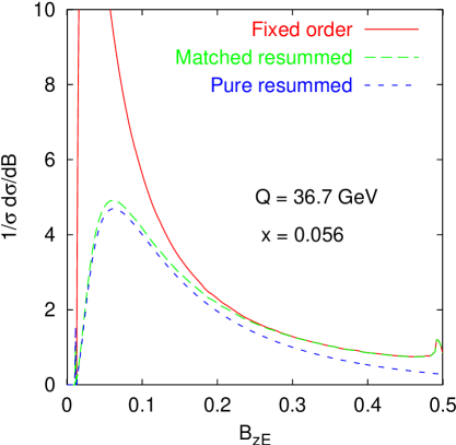
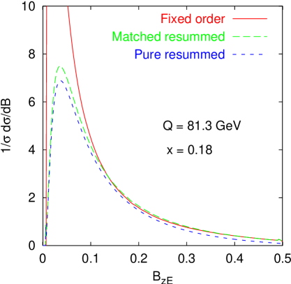
Figure 2: A comparison of fixed order, resummed and matched-resummed distributions, at two $x,Q$ values for which measurements exist at HERA [9]. The standard resummation has been used, and the matching is modified $M$-matching. No non-perturbative corrections have been included.

Figure 2 compares the resummed results (with and without matching) to the fixed order ($\alpha_{{\textsc{s}}}^{2}$) prediction as calculated with DISASTER++ [28]. The two plots correspond to different $Q$ values. One sees that in the small-$B$ region the resummation has a dramatic effect and that this effect is larger still at lower $Q$ values. One also sees that the matched curves are essentially identical to the fixed-order results at large $B$, while at small $B$ the effect of matching amounts to a small modification of the pure resummed results.

Close to the upper limit of the distribution one sees a small secondary peak, most prominent at lower $x$ and $Q$ values. It seems that this structure may actually be an artifact of the interpolation of the fixed-order distribution, since there are arguments that suggest that close to the maximum the distribution has an integrable, $(\mbox{\small$\frac{1}{2}$}-B)^{-1/2}$, divergence: when there is a single particle in the current hemisphere, at an angle $\theta$ with respect to the photon axis, the broadening is $B=\mbox{\small$\frac{1}{2}$}\sin\theta$. For $\theta$ close to $\pi/2$ there is roughly a uniform distribution of $\theta$ values, then this translates into a $(\mbox{\small$\frac{1}{2}$}-B)^{-1/2}$ behaviour for the distribution of $B$. In practice this divergence will almost certainly be smoothed out by soft gluon radiation, but that is beyond the scope of this paper.

If we calculate the matched curves with DISENT [37] (the program is much faster, but is known to give wrong subleading logarithms of $B$ [11]) we find that the results are modified by an amount of the order of a percent (for the lower $Q$ value). This small difference is a consequence of the matching that we have used: in the small-$B$ region the matching terms are multiplied by a Sudakov form factor, and therefore so are the discrepancies in DISENT. If the matching term were not multiplied by a form factor (as for example would be the case in $R$ matching) then the discrepancy would be considerably larger, of the order of $6\%$ in the peak region — however given the difficulty of carrying out $R$ matching in DIS, this is unlikely to pose a problem.

Finally we note that at the higher $Q$ value shown there could be some non-negligible contribution from $Z$-boson (rather than photon) exchange. From the point of view of the resummation this makes no difference, but for the non-logarithmically enhanced parts of the fixed order calculation there could be an effect. Unfortunately of the fixed-order programs that are able to calculate the broadening distribution with reasonable accuracy, DISENT and DISASTER++, neither implements $Z$-boson exchange.

6.2 Resummation variants

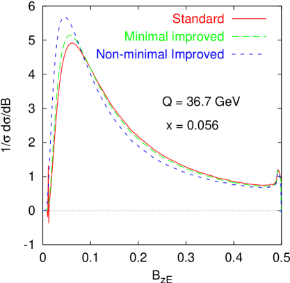
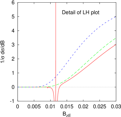
Figure 3: A comparison of the standard, ‘improved’ and ‘minimal improved’ kinds of resummations. The right hand plot shows the same curves as the left-hand plot but with a magnified abscissa. All curves use modified $M$-matching and are shown without non-perturbative corrections.

Figure 3 shows the three different varieties of resummation that have been developed in this paper. For the standard resummation one sees some ‘noise’ in the left-hand plot. In the right-hand plot, which simply has a higher resolution on the $B$ axis, one sees clearly the divergent structure associated with the derivative of the pole in $\Lambda$ (which has been analytically continued to give it meaning beyond $R^{\prime}=2$). At lower $Q$ values the problem is more prominent, but remains confined to a region which though formally within perturbative reach, in practice is beyond the applicability of the formulas.

We also show the two variants of the improved resummation. The minimal improved curve is actually very close to the standard resummation, while the non-minimal improved curve is somewhat different. This difference is indicative of the size of uncontrolled subleading effects. If one wishes to use an improved resummation we recommend the ‘minimal’ variant, mainly because of its similarity to the pure LL plus NLL resummation. We note also that the non-minimal improved resummation can show some small instabilities (not visible here) for $R^{\prime}\to\infty$, which arise in the derivative of the $((1+\sqrt{1+y^{2}})/4)^{-R^{\prime}}$ factor in the integrand for ${\bar{\Lambda}}_{n}$.

6.3 Comparison with data

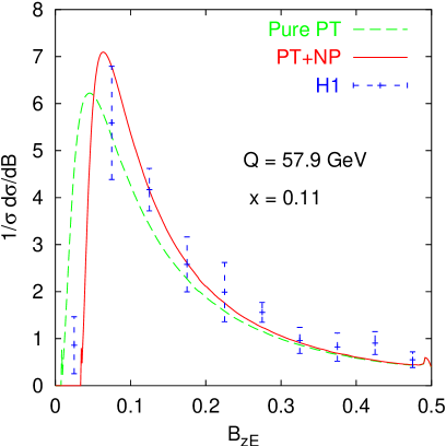
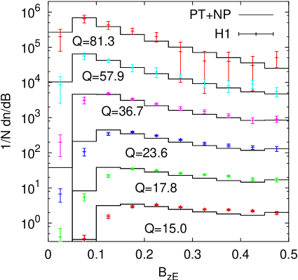
Figure 4: Comparisons of the resummed results with H1 data [9]. Experimental statistical and systematic, added in quadrature (and averaged if asymmetric). Note that in the right-hand plot the $x$ values are correlated with the $Q$ values, going from $x=0.014$ at $Q=15$ GeV, to $x=0.18$ at $Q=81.3$ GeV, and that the distributions have been rescaled by a factor $10^{i}$ with $i$ running from $0$ to $5$ respectively.

Figure 4 shows the comparison of our results to some data from H1 [9]. The left hand plot shows a single $x,Q$ value, illustrating the pure perturbative result and the prediction including the power correction (modified with $p_{\mathrm{NP}}=2$). Because of the $\ln 1/B$ dependence, the effect of the power correction is not just to shift the prediction but also to squeeze it, in a manner similar to what is seen for the $e^{+}e^{-}$ broadenings. Overall the description of the $x=0.11$ data is reasonably good (we recall that we are using standard values of $\alpha_{{\textsc{s}}}(M_{Z})=0.118$ and $\alpha_{0}=0.5$). The apparently poor description of the two lowest $B$ data points disappears in large part after integration over the bin widths.

The right-hand plot of figure 4 shows a comparison between the data and the power-corrected resummations (now integrated over bins) for a range of $x,Q$ values. There is a worsening of the description at lower values of $Q$, but this is to some extent expected, due to the increased relevance of subleading corrections (both $1/Q^{n}$ [21] and higher orders in $\alpha_{{\textsc{s}}}$).

Elsewhere [13] we shall present a more detailed analysis together with that for a range of other variables, including a study of renormalisation and factorisation scale dependence, of matching scheme and rescaling dependence (cf. appendix C), and of various other subleading effects.

7 Conclusions

For an accurate description of event shapes over the whole of the available phase space it is necessary to carry out a resummation of logarithmically enhanced terms and to supplement it with a non-perturbative correction. This paper deals with the broadening $B_{zE}$ and is one of a series addressing the resummation of a range of event shapes in the Breit-frame current hemisphere in DIS [11, 12, 13].

In principle the broadening calculations involve a straightforward extension of pre-existing resummation [4, 11] and power correction [23] techniques. In practice several subtleties arise. The standard prescription of keeping just leading and next-to-leading logarithms actually leads to a divergent answer. This divergence is associated with a change in regime: at a certain point as one goes to very small $B$, the coefficient of the double logarithm is halved, because pure Sudakov suppression stops being the favoured mechanism for producing the small $B$ values and is partially replaced by a cancellation of recoil between multiple emissions.

In principle the divergence occurs inside the region which is supposed to be under control. Accordingly we have developed techniques for extending the resummation into the region with the divergence. It is then necessary to modify our ‘accuracy criterion’ — rather than being the correct treatment of LL and NLL terms, it becomes that for $\alpha_{{\textsc{s}}}\ln 1/B\sim 1$ the distribution should be under control up to (but not including) corrections of relative order ${\alpha_{{\textsc{s}}}}$ (for normal variables these two conditions are equivalent).

In practice the divergence lies in a region where relative corrections of ${\cal{O}}\left(\alpha_{{\textsc{s}}}\right)$ are multiplied by such large (purely numerical) coefficients that the distribution is in any case not well constrained. Accordingly phenomenology is restricted to a region of larger $B$, where it turns out to be sufficient to use the ‘standard’ resummation approach. We note however that the techniques developed here may be applicable to other variables such as the difference between jet masses in $e^{+}e^{-}$ where a similar divergence is likely to be present inside the phenomenologically relevant region.

We have also made other developments which are necessary for practical phenomenology. In $e^{+}e^{-}$ there exist two standard techniques for matching the fixed order and resummed calculations. In DIS one of them ($R$-matching) is awkward to apply because of difficulties in extracting the required fixed-order information from Monte Carlo programs such as DISENT and DISASTER++. Another procedure, $\log R$ matching is applicable, but needs to be modified to address some subtleties that arise in DIS but not in $e^{+}e^{-}$. Furthermore we give details on the matching procedure proposed in [11], naming it $M$-matching, and also propose a new procedure, $M_{2}$ matching.

For the numerical implementation of our resummed formulae it was useful to develop a software tool for the evolution of parton distributions. A by product of this work was the discovery of bugs in the NLO evolution embodied in the MRST (at small $x$) and CTEQ (in the DIS scheme) parton distributions. In due course a stand-alone version of the evolution program will be made public.

Another software development, which will be discussed in detail in [13], is a tool which exploits factorisation to allow fixed-order Monte Carlo events at a single value of $x,Q$ to be reused for other $x,Q$ values. For DISASTER++ in particular this allows a gain of an order of magnitude in speed and was essential for the generation of the fixed order distributions used throughout this paper.

With the availability of these tools we have therefore for the first time been able to evaluate the resummed distribution of a DIS event shape including NLO matching and compare the results to data. We find reasonable agreement especially at higher $x$ and $Q$ values. More detailed analysis, including the study of other variables, will be presented in forthcoming work [13].

Finally we note that the programs to calculate the resummed broadening distribution, including the matching and power correction, are available from the following web page: http://cern.ch/gsalam/disresum/.

Appendix A Formulae for the radiators

We write the radiators eq. (2.18) to NLL accuracy as $R(1/B)=LR_{1}(\alpha_{{\textsc{s}}}L)+R_{2}(\alpha_{{\textsc{s}}}L)$ with

$$R_{1}(\alpha_{{\textsc{s}}}L)=\frac{C_{F}}{2\pi\beta_{0}\lambda}\left(-2\lambda-\ln(1-2\lambda)\right),$$ (A.1)

and

$$R_{2}(\alpha_{{\textsc{s}}}L)=\frac{3C_{F}}{4\pi\beta_{0}}\ln(1-2\lambda)+\frac{C_{F}K}{4\pi^{2}\beta_{0}^{2}}\frac{2\lambda+(1-2\lambda)\ln(1-2\lambda)}{1-2\lambda}\\ +\frac{C_{F}\beta_{1}}{2\pi\beta_{0}^{3}}\left(-\frac{2\lambda+\ln(1-2\lambda)}{1-2\lambda}-\frac{1}{2}\ln^{2}(1-2\lambda)\right),$$ (A.2)

where $\lambda=\alpha_{{\textsc{s}}}\beta_{0}L$ and $L=\ln 1/B$. We have defined the coefficients of the $\beta$-function to be

$$\beta_{0}=\frac{11C_{A}-2n_{\!f}}{12\pi},\qquad\quad\beta_{1}=\frac{17C_{A}^{2}-5C_{A}n_{\!f}-3C_{F}n_{\!f}}{24\pi^{2}}\,,$$ (A.3)

and the constant relating the gluon Bremsstrahlung scheme [27] to the $\overline{\mbox{\scriptsize MS}}$ to be

$$K=C_{A}\left(\frac{67}{18}-\frac{\pi^{2}}{6}\right)-\frac{5}{9}n_{\!f}\,.$$ (A.4)

For the radiator including the anomalous dimension, $R_{\gamma}$ we have

$$R_{\gamma 1} =R_{1}\,,$$ (A.5)

$$R_{\gamma 2} =R_{2}-\frac{\boldsymbol{\gamma}_{N}}{2\pi\beta_{0}}\ln(1-2\lambda)\,.$$ (A.6)

We also define

$$R^{\prime}(\alpha_{{\textsc{s}}}L)\equiv\frac{d}{dL}(LR_{1}(\alpha_{{\textsc{s}}}L))=\frac{C_{F}}{\pi\beta_{0}}\frac{2\lambda}{1-2\lambda},$$ (A.7)

and

$$R^{\prime}_{2}(\alpha_{{\textsc{s}}},L)\equiv\frac{d}{dL}(R_{2}(\alpha_{{\textsc{s}}}L))=\frac{\alpha_{{\textsc{s}}}}{2\pi}\frac{-3C_{F}}{1-2\lambda}+\frac{\alpha_{{\textsc{s}}}}{2\pi}\frac{2K\beta_{0}C_{F}\lambda-4\pi\beta_{1}C_{F}\lambda\ln(1-2\lambda)}{\pi\beta_{0}^{2}(1-2\lambda)^{2}}\,.$$ (A.8)

The analogous results for the case with the anomalous dimensions are

$$R_{\gamma}^{\prime} =R^{\prime}$$ (A.9)

$$R_{\gamma 2}^{\prime} =R_{2}^{\prime}+\frac{\alpha_{{\textsc{s}}}}{2\pi}\frac{2\boldsymbol{\gamma}_{N}}{1-2\lambda}$$ (A.10)

Finally we shall need the leading parts of the second and third derivatives:

$$R_{\gamma}^{\prime\prime}\equiv R^{\prime\prime} =\frac{2C_{F}}{\pi}\frac{\alpha_{{\textsc{s}}}}{(1-2\lambda)^{2}}\,,$$ (A.11)

$$R_{\gamma}^{\prime\prime\prime}\equiv R^{\prime\prime\prime} =\frac{8C_{F}}{\pi}\frac{\alpha_{{\textsc{s}}}^{2}\beta_{0}}{(1-2\lambda)^{3}}\,.$$ (A.12)

Appendix B Fixed order result

Here we calculate the first order coefficient function $\boldsymbol{C}_{1}$, which appears for example in (4.2). It is needed in a variety of contexts — for example in many (but not all) of the approaches to matching with fixed-order calculations, and also for carrying out comparisons down to ${\bar{\alpha}}_{{\textsc{s}}}^{2}L^{2}$ accuracy with fixed-order calculations. Calculating $\boldsymbol{C}_{1}$ proves more cumbersome in DIS than in $e^{+}e^{-}$ since instead of a pure number one obtains a function of the variable $\xi=Q^{2}/(2p.q)$, where $p$ is the four-momentum of the incoming (as opposed to struck) parton. Additionally there are various contributions to be computed, i.e. transverse and longitudinal parts of graphs with an incoming quark as well as boson gluon fusion. It proves convenient to first compute the $\mathcal{O}(\alpha_{s})$ result for events with broadening $B_{zE}>B$ because at leading order this quantity, $\sigma_{c}^{(1)}$, doesn’t get any virtual correction. Note that this is complementary to the final quantity we want, $\sigma_{r}^{(1)}$, which requires the selection of events with $B_{zE}<B$. The following relation is therefore required (which follows from unitarity)

$$\sigma_{r}^{(1)}=\sigma_{\mathrm{tot}}^{(1)}-\sigma_{c}^{(1)}\,,$$ (B.1)

where $\sigma_{\mathrm{tot}}^{(1)}$ is the total $\mathcal{O}(\alpha_{s})$ cross-section for all events, except those with an empty current hemisphere which are excluded throughout, since it does not make much sense to define current jet observables in such a situation.

The computation of $\sigma_{c}^{(1)}$ is relatively straightforward up to terms of order $B$, which we do not require, and after applying eq. (B.1) (at the level of the corresponding coefficient functions ) we obtain the following pieces relevant to the computation of $\sigma_{r}^{(1)}$

• $F_{2}$ quark contribution

  $$\mathcal{F}_{q}(B,\xi)=-\delta(1-\xi)\left[4\ln^{2}B-3\ln\frac{1}{B}-4\ln 2\ln B+2\ln^{2}2+3-3\ln 2-\frac{\pi^{2}}{3}\right]\\ -2\frac{1+\xi^{2}}{(1-\xi)_{+}}\ln\frac{1}{B}+\frac{1+\xi^{2}}{1-\xi}\ln{\xi}-(1+\xi^{2})\left(\frac{\ln{(1-\xi)}}{1-\xi}\right)_{+}+\frac{6\xi^{2}-2\xi-1}{2(1-\xi)_{+}}\,.$$ (B.2)

• $F_{2}$ gluon contribution

  $$\mathcal{F}_{g}(B,\xi)=-[\xi^{2}+(1-\xi^{2})]\left[4\ln\frac{1}{B}-2+2\ln\frac{1-\xi}{\xi}\right]-8\xi(1-\xi)\,.$$ (B.3)

Note that the longitudinal contributions are absent since they cancel in the two terms of eq. (B.1). Then we have $\sigma_{r}^{(1)}$ is given by

$$\sigma_{r}^{(1)}(x,B,Q^{2})=\frac{1}{q(x)}\,\frac{\alpha_{s}}{2\pi}\int_{x}^{1}\frac{d\xi}{\xi}\left[C_{F}\,\mathcal{F}_{q}(B,\xi)\,q(x/\xi)+T_{f}\,\mathcal{F}_{g}(B,\xi)\,g(x/\xi)\right]\,,$$ (B.4)

with

$$q(x)=\sum_{j=1}^{n_{f}}e_{j}^{2}[q_{j}(x)+\bar{q}_{j}(x)]\,,\quad T_{f}=T_{R}\sum_{j=1}^{n_{f}}e_{j}^{2}\,.$$ (B.5)

In the above $q_{j}(x)$ and $g(x)$ are quark and gluon distributions (for a quark with flavour index $j$ and corresponding charge electric charge $e_{j}$). The colour factors are as usual $C_{F}=4/3$, $T_{R}=1/2$ and $n_{f}$ denotes the number of active flavours. From the above leading order result the constant ($C_{1}$) and logarithmic ($G_{11}$ and $G_{12}$) pieces can be easily read-off. In particular the logarithms are in agreement with those obtained at this order from the resummation method. The transpose of the matrix $\boldsymbol{C}_{1}$ in section 4 is

$$\boldsymbol{C}_{1}^{T}(x)=\left(\begin{array}[]{c}e_{u}^{2}C_{1,q}(x)\\ e_{u}^{2}C_{1,q}(x)\\ \vdots\\ \sum_{q,{\bar{q}}}e_{q}^{2}C_{1,g}(x)\end{array}\right)$$ (B.6)

with

$$C_{1,q}(\xi) =C_{F}\,{\mathcal{F}}_{q}(1,\xi)\,,$$ (B.7a)

$$C_{1,g}(\xi) =\frac{T_{R}}{2}\,{\mathcal{F}}_{g}(1,\xi)\,.$$ (B.7b)

Lastly we add that the above results are valid for the DIS factorisation scheme. To go the $\overline{\mbox{\scriptsize MS}}$ scheme one should add the standard $\overline{\mbox{\scriptsize MS}}$ scheme $F_{2}$ coefficient functions to the above results exactly as in eqs. (A.9) and (A.10) in appendix A of Ref. [11].

Appendix C Rescaling the variable

Usually the resummation of a variable $V$ is defined in terms of $\ln 1/V$; however we can just as well define it in terms of $\ln 1/XV$ where $X$ is some arbitrary number. If we do this then in the resummed formula we need to make the following replacements (note that the meaning of overlined symbols, such as ${\overline{L}}$, is not in any way related to the meaning of barred symbols, ${\bar{L}}$, introduced when discussing the improved resummation):

$$L \to{\overline{L}}=\ln\frac{1}{XV}\,,$$ (C.1)

$$g_{1}(\alpha_{{\textsc{s}}}L) \to g_{1}(\alpha_{{\textsc{s}}}{\overline{L}})\,,$$ (C.2)

$$g_{2}(\alpha_{{\textsc{s}}}L) \to g_{2}(\alpha_{{\textsc{s}}}{\overline{L}})+(g_{1}(\alpha_{{\textsc{s}}}{\overline{L}})+\alpha_{{\textsc{s}}}{\overline{L}}g_{1}^{\prime}(\alpha_{{\textsc{s}}}{\overline{L}}))\ln X\,,$$ (C.3)

where bold symbols for those functions that are operators in $x$ and flavour space.

We also need to modify the constant term:

$$C_{1}\to{\overline{C}}_{1}=C_{1}+G_{12}\ln^{2}X+G_{11}\ln X$$ (C.4)

In the fixed order expansion there are corresponding modifications which need to be taken into account:

$$G_{11} \to{\overline{G}}_{11}=G_{11}+2G_{12}\ln X$$ (C.5)

$$G_{22} \to{\overline{G}}_{22}=G_{22}+3G_{23}\ln X$$ (C.6)

which imply the following modifications at orders $\alpha_{{\textsc{s}}}$

$$\sigma^{(1)}_{r}(L)\to\sigma^{(1)}_{r}({\overline{L}})+\Delta G_{11}L+\Delta C_{1}\,,$$ (C.7)

and $\alpha_{{\textsc{s}}}^{2}$:

$$\sigma^{(2)}_{r}(L)\to\sigma^{(2)}_{r}({\overline{L}})+G_{12}\Delta G_{11}L^{3}+\\ +\left(\Delta G_{22}+G_{11}\Delta G_{11}+\mbox{\small$\frac{1}{2}$}(\Delta G_{11})^{2}+G_{12}\Delta C_{1}\right)L^{2}+\\ +\left(G_{11}\Delta C_{1}+\Delta G_{11}C_{1}+\Delta G_{11}\Delta C_{1}\right)L\,.$$ (C.8)

We have defined $\Delta C_{1}={\overline{C}}_{1}-C$ and similarly for other quantities. This expansion is valid in the case where $C_{1}$ multiplies $q(V^{n}Q^{2})$ rather than $q(Q^{2})$ as was used in [11]. However the analogous expressions are straightforward to determine for that case too.

The above formulae follow directly from the $N$ space resummed result but their re-interpretation, where required, as matrix projections in $x$ space is rather straightforward. We note that these formulae are currently not applicable to the improved broadening resummations, which have further terms that need to be taken into account.

Appendix D Accuracy checks

In deriving the ‘improved’ resummation in section 3, the stated aim was that the result should be correct to within corrections of relative order $\alpha_{{\textsc{s}}}$. This requires a careful study of contributions that have been neglected.

There are three main potential sources of inaccuracy that must be considered:

• The choice of the expansion point.

• The terms to be kept in the expansion of $R_{\gamma}$ (and whether they need to be kept in the exponent).

• The choice of terms needed in evaluating the derivative of $\ln\sigma$, required for the inverse $\nu$-transform.

D.1 Choice of expansion point

In the standard approach of section 2 the radiators are both expanded around the point $\nu$. If one’s only interest were to obtain a convergent answer for $R^{\prime}\gtrsim 2$ then this could be achieved by keeping that expansion point and simply including the second order expansion of $R$ in the exponent.

However for $R^{\prime}>2$ the saddle-point of the integral is far from $bQ\sim\nu$. Indeed it is in a region where $\alpha_{{\textsc{s}}}\ln\nu/bQ\sim 1$, and therefore in an expansion

$$R(bQ)=R(\nu)+\sum_{n=1}^{\infty}R^{(n)}\left(\ln\frac{bQ}{\nu}\right)^{n}$$ (D.1)

where $R^{(n)}(\nu)$ is of the form $\alpha_{{\textsc{s}}}^{n-1}f(\alpha_{{\textsc{s}}}L)$, it is necessary to keep all terms. One way this could be achieved, is by not expanding in the first place and integrating, say numerically, over $b$ with the full function for $R(b)$. However this would lead to problems because for sufficiently large values of $b$ one reaches a singularity associated with the Landau pole in $R$.

If on the other hand we expand close to the saddle-point of the integral the situation simplifies. The width of the integrand around the saddle-point is roughly of order $1/\sqrt{R^{\prime\prime}}\sim\alpha_{{\textsc{s}}}^{-1/2}$, allowing us to keep a fixed number of terms in our expansion.

For simplicity we choose to expand not around the actual saddle point, but a point $b_{0}$ close to it, differing from it by a pure numerical factor. Since in any case we will then have to keep terms in our expansion so as to give an accurate representation of our function up to $\ln b/b_{0}\sim\alpha_{{\textsc{s}}}^{-1/2}$, the difference of a pure factor between the expansion and saddle points makes no difference.

D.2 Choice of terms to be kept

When examining the choice of terms to be kept, the discussion can be kept simpler in the relevant region, $\alpha_{{\textsc{s}}}L\sim 1$, by noting that any quantity which is formally $\alpha_{{\textsc{s}}}^{n}f(\alpha_{{\textsc{s}}}L)$ (with $f$ some arbitrary function) is just of order $\alpha_{{\textsc{s}}}^{n}$. Accordingly we will refer to $R^{\prime\prime}$ as being of order $\alpha_{{\textsc{s}}}$, $R^{\prime\prime\prime}$ as being of order $\alpha_{{\textsc{s}}}^{2}$ and so on.

Keeping the first and second order terms in the expansion of ${\cal{R}}_{R}$, our basic integral is of the form

$$\lambda=\int\frac{dy}{y}\frac{y^{2}}{(1+y^{2})^{3/2}}\left(\frac{1+\sqrt{1+y^{2}}}{4}\right)^{-R^{\prime}}e^{-(\ln\frac{y}{2}-\ell){\bar{R}}^{\prime}-\frac{1}{2}(\ln\frac{y}{2}-\ell)^{2}{\bar{R}}^{\prime\prime}}\,.$$ (D.2)

We see that for ${\bar{R}}^{\prime}\simeq 2$ it is the ${\bar{R}}^{\prime\prime}$ term which ensures the integral’s convergence. It must therefore be kept in the exponent. Examining the integral one sees that there are actually three possible regimes.

• $2-R^{\prime}\gg\sqrt{\alpha_{{\textsc{s}}}}$. In this case the expansion point remains close to $y=1$ and the integral converges in a region of $\Delta\ln y$ of order $1$.

• $2-R^{\prime}\sim\sqrt{\alpha_{{\textsc{s}}}}$. In this case the saddle and expansion points remain close to $y=1$. The relevant integration region extends down to $\ln y\sim-\alpha_{{\textsc{s}}}^{-1/2}$, but convergence is rapid for $y>1$.

• $R^{\prime}-2\gg\sqrt{\alpha_{{\textsc{s}}}}$. Here $-\ell\gg\sqrt{\alpha_{{\textsc{s}}}}$ and accordingly the relevant part of the integral is entirely contained in the region $y\ll 1$ and all occurrences of $1+y^{2}$ can simply be replaced by $2$.

The first region is simply that addressed in section 2, and one can neglect even the $R^{\prime\prime}$ term.

The second and third regions require more care. We need to understand what happens when we multiply the integrand by a term $\alpha_{{\textsc{s}}}^{m}(\ln y-\ell)^{n}$,

$$\lambda_{mn}=\int\frac{dy}{y}\frac{y^{2}}{(1+y^{2})^{3/2}}\left(\frac{1+\sqrt{1+y^{2}}}{4}\right)^{-R^{\prime}}e^{-(\ln\frac{y}{2}-\ell){\bar{R}}^{\prime}-\frac{1}{2}(\ln\frac{y}{2}-\ell)^{2}{\bar{R}}^{\prime\prime}}\cdot\alpha_{{\textsc{s}}}^{m}\left(\ln\frac{y}{2}-\ell\right)^{n}\,.$$ (D.3)

Let us first consider the third region, where this simplifies to

$$2^{2+R^{\prime}}e^{2\ell}\int\frac{dy}{y}e^{-(\ln\frac{y}{2}-\ell)({\bar{R}}^{\prime}-2)-\frac{1}{2}(\ln\frac{y}{2}-\ell)^{2}{\bar{R}}^{\prime\prime}}\cdot\alpha_{{\textsc{s}}}^{m}\left(\ln\frac{y}{2}-\ell\right)^{n}\,.$$ (D.4)

If we are sufficiently into this region that we can neglect the $({\bar{R}}^{\prime}-2)$ term then we obtain

$$\frac{\lambda_{mn}}{\lambda}\sim\left\{\begin{array}[]{ll}\alpha_{{\textsc{s}}}^{m-n/2}&\mbox{$n$ even}\\ 0&\mbox{$n$ odd}\end{array}\right.$$ (D.5)

The largest such contributions will come from terms such as $(R_{\gamma 2}^{\prime})^{2}$, ${R^{\prime\prime\prime}}^{2}$, $R^{(4)}$, and will all be of relative order $\alpha_{{\textsc{s}}}$, and so negligible.

In the situation where $2-R^{\prime}\sim\sqrt{\alpha_{{\textsc{s}}}}$ the situation is more complex because the odd-$n$ terms do not give zero. The reason is that the integral extends only to one side of the saddle-point so one loses the cancellation between $\ln y/2-\ell>0$ and $\ln y/2-\ell<0$. Accordingly, in this region

$$\frac{\lambda_{mn}}{\lambda}\sim\alpha_{{\textsc{s}}}^{m-n/2},\qquad n\geq 0\,.$$ (D.6)

Accordingly we must keep all terms $\alpha_{{\textsc{s}}}(\ln y/2-\ell)$ and $\alpha_{{\textsc{s}}}^{2}(\ln y/2-\ell)^{3}$, since they contribute at the relative ${\cal{O}}\left(\sqrt{\alpha_{{\textsc{s}}}}\right)$ level. This is the motivation behind the set of terms kept in eq. (3.6).

D.3 Terms to be kept in the derivative of $\boldsymbol{{\bar{\Lambda}}}$

In evaluating the inverse Mellin transform with respect to $\nu$, it is necessary to calculate the factor

$$\frac{1}{\Gamma\left(1+\nu\frac{d}{d\nu}\ln\sigma\right)}\,.$$ (D.7)

In the second and third regions discussed above ${\bar{\Lambda}}$ varies rapidly, so its derivative can contribute significantly to this factor and should not be neglected.

The derivative of the full $\ln{\bar{\Lambda}}$ is technically quite complicated to evaluate because of the presence of the anomalous-dimension matrices. However these terms, which are of order $\alpha_{{\textsc{s}}}(\ln y/2-\ell)$, have two important features: they give a contribution of relative order $\sqrt{\alpha_{{\textsc{s}}}}$, and that contribution is relevant (and varies significantly) only in the region of $\Delta L\sim\alpha_{{\textsc{s}}}^{-1/2}$. Consequently in $\ln{\bar{\Lambda}}$ when taking the derivative with respect to $L$, these extra pieces become of order $\alpha_{{\textsc{s}}}$ rather than $\sqrt{\alpha_{{\textsc{s}}}}$, and so can be neglected. The same is true of all terms which contribute a relative amount $\sqrt{\alpha_{{\textsc{s}}}}$ in this limited region of $L$.

The fact that we can throw away terms contributing a relative amount $\sqrt{\alpha_{{\textsc{s}}}}$ in that region also allows us to modify the large-$y$ structure of the integrand, and therefore we can use ${\bar{\Lambda}}_{m}$ rather than ${\bar{\Lambda}}_{n}$. That the large-$y$ region contributes an amount of relative order $\sqrt{\alpha_{{\textsc{s}}}}$ follows from the fact that the whole integral is of order $\alpha_{{\textsc{s}}}^{-1/2}$, while the large-$y$ region is unenhanced and contributes an amount of order $1$.

Appendix E Modified matching

As was discussed in section 4, it is important that the matching respect certain properties concerning the behaviour at the maximum of the distribution $V=V_{\mathrm{max}}$. We recall that these were: first the integrated cross section should go to whatever the correct upper limit happens to be, without leftover terms of order $\alpha_{{\textsc{s}}}^{3}$ or higher. Secondly if the fixed order distribution goes to zero smoothly at the upper limit, so should the matched-resummed one. In $e^{+}e^{-}$ this was always the case, whereas for many DIS variables the distribution is non-zero at the upper limit (and the upper limit is the same for all orders). Here we discuss a modified matching procedure that makes sure that the final answer has the required behaviour in the above respects.

The first element of the modification is to replace

$$L=\ln\frac{V_{0}}{V}\to{\widetilde{L}}=\frac{1}{p}\ln\left[\left(\frac{V_{0}}{V}\right)^{p}-\left(\frac{V_{0}}{V_{\mathrm{max}}}\right)^{p}+1\right]\,,$$ (E.1)

where we have generalised through the inclusion of the power $p$ the modification originally proposed in [1] (which used $p=1$). Typically one might expect to consider $1\leq p\lesssim 3$, where the upper limit is fairly arbitrary and the lower one comes from an assumption that the cross section contains no terms of the form $V^{p}\ln V$ with $p<1$. In cases where we use a rescaled variable then we have

$${\overline{L}}=\ln\frac{V_{0}}{XV}\to{\widetilde{\overline{L}}}=\frac{1}{p}\ln\left[\left(\frac{V_{0}}{XV}\right)^{p}-\left(\frac{V_{0}}{XV_{\mathrm{max}}}\right)^{p}+1\right]\,.$$ (E.2)

We shall also need a factor with the property that it goes to $1$ rapidly for $V\to 0$ and to zero for $V=V_{\mathrm{max}}$. We adopt the following form for it:

$$Z(V)=1-\left(\frac{V}{V_{\mathrm{max}}}\right)^{p}.$$ (E.3)

For $M$ and $M_{2}$ matching, the replacement of $L$ with ${\widetilde{L}}$ is usually sufficient to ensure that cross section goes exactly to the ${\cal{O}}\left(\alpha_{{\textsc{s}}}^{2}\right)$ upper limit. This is because at $V=V_{\mathrm{max}}$, ${\widetilde{L}}=0$, and accordingly $\sigma_{r}$ contains no terms higher than ${\cal{O}}\left(\alpha_{{\textsc{s}}}\right)$, and the matching adjusts both the order $\alpha_{{\textsc{s}}}$ and $\alpha_{{\textsc{s}}}^{2}$ terms to be exact, without introducing any additional terms. There is an exception to this rule for the improved broadening formula, which contains ${\cal{O}}\left(\alpha_{{\textsc{s}}}^{3}\right)$ terms at $V_{\mathrm{max}}$ even after the replacement $L\to{\widetilde{L}}$ — these then need to be subtracted.

If $\sigma^{(2)}_{e}(V_{\mathrm{max}})$ is non-zero (as it usually is), then the matched distribution does not go to zero even if the fixed order one does, because of the ${\bar{\alpha}}_{{\textsc{s}}}^{3}\sigma^{(2)}_{e}(V_{\mathrm{max}})\mathcal{G}_{11}$ contribution. Technically the most straightforward solution to the above two problems is to use the following formula

$$\sigma(V)=\sigma_{r}+\left[{\bar{\alpha}}_{{\textsc{s}}}\left(\sigma_{e}^{(1)}-\sigma_{r}^{(1)}\right)+{\bar{\alpha}}_{{\textsc{s}}}^{2}\left(\sigma_{e}^{(2)}-\sigma_{r}^{(2)}\right)-{\bar{\alpha}}_{{\textsc{s}}}^{2}Z(V)\left(\sigma_{e}^{(1)}-\sigma_{r}^{(1)}\right)(L^{2}G_{12}+L\mathcal{G}_{11})\right.\\ \left.+1+{\bar{\alpha}}_{{\textsc{s}}}\sigma_{r}^{(1)}(V_{\mathrm{max}})+{\bar{\alpha}}_{{\textsc{s}}}^{2}\sigma_{r}^{(2)}(V_{\mathrm{max}})-\sigma_{r}(V_{\mathrm{max}})\right]\Sigma^{Z(V)}\,,$$ (E.4)

though strictly speaking only the $G_{11}$ part of $\Sigma$ need be raised to the power $Z(V)$.

Correspondingly for $M_{2}$ matching we have

$$\sigma(V)=\sigma_{r}+{\bar{\alpha}}_{{\textsc{s}}}\left(\sigma_{e}^{(1)}-\sigma_{r}^{(1)}\right)+\left[{\bar{\alpha}}_{{\textsc{s}}}^{2}\left(\sigma_{e}^{(2)}-\sigma_{r}^{(2)}\right)\right.\\ \left.+1+{\bar{\alpha}}_{{\textsc{s}}}\sigma_{r}^{(1)}(V_{\mathrm{max}})+{\bar{\alpha}}_{{\textsc{s}}}^{2}\sigma_{r}^{(2)}(V_{\mathrm{max}})-\sigma_{r}(V_{\mathrm{max}})\right]\Sigma^{Z(V)}\,.$$ (E.5)

For $\ln R$ matching the situation is different in that, following the replacement $L\to{\widetilde{L}}$, the matched distribution goes to zero if the fixed-order one does, but that now we need to fix up the value of the cross section at the upper limit. In this respect the procedure differs from the $e^{+}e^{-}$ case, where replacing $L\to{\widetilde{L}}$ led to all required properties automatically being satisfied. There are two reasons for the difference: the fact that we keep the full $\sigma_{rq}$ in front of the exponential (in $e^{+}e^{-}$ the constant part is left out) and the fact that the fixed order cross section does not go to exactly $1$ at the upper limit, but to $1+{\cal{O}}\left(\alpha_{{\textsc{s}}}\right)$. To ensure that we get exactly the same answer as the ${\cal{O}}\left(\alpha_{{\textsc{s}}}^{2}\right)$ answer we need to insert an extra factor $F$ in front of the exponential:

$$\sigma(V)=\sigma_{rg}+\sigma_{rq}\,F\,e^{{\bar{\alpha}}_{{\textsc{s}}}\left(\sigma^{(1)}_{e}-\sigma^{(1)}_{r}\right)+{\bar{\alpha}}_{{\textsc{s}}}^{2}\left(\sigma^{(2)}_{e}-\sigma^{(2)}_{r}-\frac{1}{2}\left(\sigma^{(1)}_{e}-\sigma^{(1)}_{r}\right)\left(\sigma^{(1)}_{e}+\sigma^{(1)}_{r}-2\sigma^{(1)}_{rg}\right)\right)}\,,$$ (E.6)

with

$$F=e^{-{\bar{\alpha}}_{{\textsc{s}}}\left(\sigma^{(1)}_{e}-\sigma^{(1)}_{r}\right)-{\bar{\alpha}}_{{\textsc{s}}}^{2}\left(\sigma^{(2)}_{e}-\sigma^{(2)}_{rq}-\frac{1}{2}\left(\sigma^{(1)}_{e}-\sigma^{(1)}_{r}\right)\left(\sigma^{(1)}_{e}+\sigma^{(1)}_{r}-2\sigma^{(1)}_{rg}\right)\right)}\\ \left.\frac{1+{\bar{\alpha}}_{{\textsc{s}}}(\sigma^{(1)}_{e}-\sigma^{(1)}_{rg})+{\bar{\alpha}}_{{\textsc{s}}}^{2}\sigma^{(2)}_{e}}{1+{\bar{\alpha}}_{{\textsc{s}}}\sigma^{(1)}_{rq}+{\bar{\alpha}}_{{\textsc{s}}}^{2}\sigma^{(2)}_{rq}}\right|_{V=V_{\mathrm{max}}}\,.$$ (E.7)

where have exploited the fact that $\sigma^{(2)}_{rg}(V_{\mathrm{max}})$ is zero. Since $F=1+{\cal{O}}\left(\alpha_{{\textsc{s}}}^{3}\right)$ the inclusion of the factor $F$ makes no difference (at our accuracy) to the small-$V$ behaviour of the answer.

To see that the matched distribution goes to zero if the fixed-order one does, we restrict ourselves to the case of variables without any variable dependent scale in the structure function, because it turns out that none of the variables involving $V$ in the scale of the distribution have fixed-order distributions which go to zero at the upper limit. So with this proviso one recalls

$$\sigma_{rq}=(1+{\bar{\alpha}}_{{\textsc{s}}}{\mathcal{C}}_{1})e^{{\widetilde{L}}g_{1}(\alpha_{{\textsc{s}}}{\widetilde{L}})+g_{2}(\alpha_{{\textsc{s}}}{\widetilde{L}})}\,\qquad\quad{\mathcal{C}}_{1}=\frac{\boldsymbol{C}_{1}\otimes\boldsymbol{q}}{q}\,.$$ (E.8)

In the exponent, after matching, the $\alpha_{{\textsc{s}}}$ and $\alpha_{{\textsc{s}}}^{2}$ will have vanishing derivatives by construction (i.e. from the inclusion of the fixed order pieces). At order $\alpha_{{\textsc{s}}}^{3}$ we get contribution only from $g_{1}$ and $g_{2}$, but they go as ${\widetilde{L}}^{4}$ and ${\widetilde{L}}^{3}$ respectively and accordingly their derivatives vanish. This ensures that the quark resummation part gives a vanishing distribution.

We also need to show that the gluon resummation piece gives a vanishing distribution — this follows since, because we have included no $g_{2}$ term in the gluon resummation exponent, the lowest power of ${\widetilde{L}}$ that is present is ${\widetilde{L}}^{2}$, automatically giving zero derivative.

Appendix F Parton distributions

A complication in the practical computation of the broadening (and also $\tau_{zE}$ and $\tau_{zQ}$) distribution in DIS arises from the fact that the main result (2.26) involves operators in $x$ and flavour space, a consequence of the presence of the anomalous dimension matrix, $\boldsymbol{\gamma}_{N}$, in $R_{\gamma}$.

The action of $\boldsymbol{\gamma}_{N}$ is of course just to change the scale of the parton distributions to $(VQ)^{2}$, i.e. we can rewrite (2.26) as

$$\Sigma_{N}(B)=\boldsymbol{C}_{0,N}\frac{\Lambda(2R^{\prime})}{\Gamma(1+2R^{\prime})}e^{-2R(1/B)-R^{\prime}(\ln 2+2\gamma_{E})}\boldsymbol{q}_{N}(V^{2}Q^{2})\,.$$ (F.1)

Parton distributions are available in tabulated form as a function of scale from groups such as MRST [26], CTEQ [24] or GRV [25], so we could just choose to use these tabulated distributions at scale $V^{2}Q^{2}$. This is what is usually done in the context for example of Drell-Yan $p_{t}$ resummations (for recent examples, see [38] and references therein).

Instead however we have chosen to take a seemingly more complicated route and develop our own software for the evolution of parton distributions. There are four main reasons for this.

Matching.

When we carry out matching to fixed-order calculations we need to know quantities such as

$$\boldsymbol{P}^{(1)}\otimes q\,,\qquad\boldsymbol{P}^{(2)}\otimes q\,,\qquad\boldsymbol{P}^{(1)}\otimes\boldsymbol{P}^{(1)}\otimes q\,,$$ (F.2)

where $\boldsymbol{P}^{(1)}$ and $\boldsymbol{P}^{(2)}$ are the matrices respectively of leading and next-to-leading order splitting functions. By taking numerical derivatives it would be possible to obtain certain combinations of the above quantities, for example

$$\left({\bar{\alpha}}_{{\textsc{s}}}\boldsymbol{P}^{(1)}+{\bar{\alpha}}_{{\textsc{s}}}^{2}\boldsymbol{P}^{(2)}\right)\otimes q$$ (F.3)

from the first derivative. However this combination would be obtained only for a particular value of $\alpha_{{\textsc{s}}}$ (that used in the original evolution). The double convolution term can be obtained from the second derivative of the structure functions, but only in a form ‘polluted’ by additional ${\cal{O}}\left(\alpha_{{\textsc{s}}}^{3}\right)$ terms. Furthermore some current tabulated (global fit) parton distribution sets use quite poor interpolation which means that numerically determined derivatives (especially higher derivatives) are nonsensical.

So we in any case need to write software to calculate the quantities in (F.2). Once this is done, writing a full PDF evolution program involves relatively little extra work.

Flexibility.

If we follow the philosophy of $e^{+}e^{-}$ event-shape resummations, i.e. we include LL and NLL terms but no higher-order contributions (other than as introduced in the matching), then we must take eq. (2.26) literally, using only the leading-order splitting functions. If on the other hand we use (F.1) with tabulated global-fit parton distributions then the evolution embodied in $q(V^{2}Q^{2})$ will automatically include NLO splitting functions (either way we have to use NLO parton densities since we match to ${\cal{O}}\left(\alpha_{{\textsc{s}}}^{2}\right)$ fixed order calculations).

Using our own evolution code gives us a certain flexibility, and we are free to take a NLO parton distribution at scale $Q$, and then apply to it the operator $\exp(-R_{\gamma}(B))$, i.e. carry out leading order evolution to scale $VQ$.

Fitting $\boldsymbol{\alpha_{{\textsc{s}}}}$.

When fitting for $\alpha_{{\textsc{s}}}$, for each new value of $\alpha_{{\textsc{s}}}$ that one wishes to examine, the formally correct procedure is to reevaluate all quantities using parton distributions fitted with that value of $\alpha_{{\textsc{s}}}$.

With the tools that are currently available for calculating fixed-order distributions, this means rerunning DISENT or DISASTER++, a process which can use several tens of days of computing time on a modern workstation. As a result it is common to fit for $\alpha_{{\textsc{s}}}$ using a single PDF set and then to check that the results do not change significantly with a set corresponding to a different value of $\alpha_{{\textsc{s}}}$.

Within this approach, if we insert tabulated global-fit distributions into (F.1), then while most of the calculation will be done with the value of $\alpha_{{\textsc{s}}}$ that is explicitly inserted into the formulas, the single logs associated with the anomalous dimension will be evaluated with a value of $\alpha_{{\textsc{s}}}$ corresponding to the PDF set. We can study the extent to which this is a problem by examining how the ratio

$$\frac{q(x,V^{2}Q^{2})}{q(x,Q^{2})}$$ (F.4)

depends on different approaches used for its evaluation (we recall our earlier definition for $q$, eq. (4.4)). Suppose we are calculating the broadening distribution with $\alpha_{{\textsc{s}}}(M_{Z})=0.1225$. The correct procedure is to calculate the ratio (F.4) using the MRST99 hi-$\alpha_{{\textsc{s}}}$ ($\alpha_{{\textsc{s}}}(M_{Z})=0.1225$) set evolved down from $Q$ to $VQ$ with this appropriate value of $\alpha_{{\textsc{s}}}(M_{Z})$. We want to examine the error that is made if one calculates this ratio in two different ways (as would be done in a fit): (a) with the central-$\alpha_{{\textsc{s}}}$ MRST99 (originally fitted with $\alpha_{{\textsc{s}}}(M_{Z})=0.1175$) set evaluated at scale $Q^{2}$ and evolved down to $V^{2}Q^{2}$ with $\alpha_{{\textsc{s}}}(M_{Z})=0.1175$ — this is roughly equivalent to using the ‘central’ tabulated global-fit distribution in both the numerator and denominator of (F.1); (b) with the central-$\alpha_{{\textsc{s}}}$ MRST99 set evaluated at scale $Q^{2}$ and evolved down to $V^{2}Q^{2}$ with $\alpha_{{\textsc{s}}}(M_{Z})=0.1225$ — this is the philosophy of treating the anomalous dimension terms on the same footing as all the other single logs. The error that arises in these two different approaches is shown in figure 5, where one sees that the $\alpha_{{\textsc{s}}}$ used in the evolution is considerably more important than the $\alpha_{{\textsc{s}}}$ used in the fit for the parton distributions.

It should however be noted that for small-$x$ and small-$Q$ we can have the opposite situation because of the strong correlation between the value of $\alpha_{{\textsc{s}}}$ and the fitted gluon distribution. Nevertheless this analysis indicates that at the very least we want the option of doing our own evolution of the parton distribution.

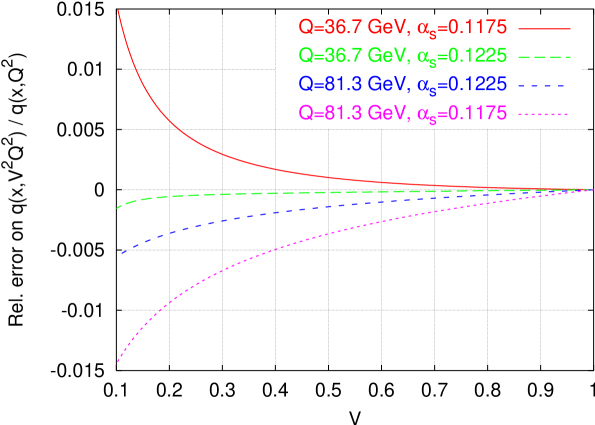
Figure 5: The relative error on the ratio (F.4) introduced by (improper) use of the central MRST PDF set to calculate quantities at $\alpha_{{\textsc{s}}}(M_{Z})=0.1225$ (where one should formally use the high-$\alpha_{{\textsc{s}}}$ MRST distribution). Shown for $x=0.056,\,Q=36.7$ GeV and $x=0.18,\,Q=81.3$ GeV. The value of $\alpha_{{\textsc{s}}}$ is that used to evolve the central MRST parton distribution down from scale $Q^{2}$ to scale $V^{2}Q^{2}$.

Technical limitations of tabulated global-fit distributions.

One final motivation for using our evolution in calculating is $q(V^{2}Q^{2})$ is smoothness. Generally global-fit parton distributions are provided in tabulated form together with an interpolating program.

In the case of the CTEQ and GRV distributions the interpolation is of reasonable quality. However for the current publicly available MRST distributions (dating from 1999, [26]) only linear interpolation is used, leading to non-smoothness in $Q$. When calculating a resummed distribution (as opposed to the integrated cross section) one takes the derivative of (F.1) and this non-smoothness gets promoted to discontinuities. This is illustrated in figure 6 which shows the broadening distribution for $Q=81.3$ GeV, determined in two ways: in one case we have used our own evolution between scales $Q$ and $VQ$; in the other case we have used the MRST99 tabulated distributions to obtain $q(V^{2}Q^{2})$. The clear discrepancies between the two curves (at the level of a few percent) are a consequence of the non-smoothness of the tabulated distribution.

We have also tested a preliminary version of the MRST 2001 distributions [39], which use improved interpolation code, and there we find that the problem is eliminated.

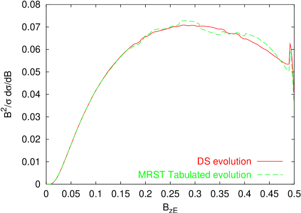
Figure 6: The broadening distribution (without power correction) calculated using our own (DS) evolution and with the MRST99 tabulated evolution. Shown for $x=0.18,\,Q=81.3$ GeV. For other $x,Q$ points of interest at HERA, the non-smoothness of the MRST distributions has a smaller effect. A leading factor of $B^{2}$ has been included so as to highlight the large-$B$ region, where the problem is more severe.

F.1 Convolution and evolution algorithms.

We have seen above that there are several motivations for evolving the parton distributions independently from the original global-fit tabulations. Accordingly we have developed our own evolution and convolution code. Various requirements arise from the need to use it for event shape resummations (though we envisage that it may well have wider applications):

• Flexibility: it should be straightforward to implement new kernels (i.e. without any special analytical work), since each event shape involves a new constant piece $C_{1}$. This also makes it straightforward to extend it to NNLL evolution.

• Reasonable tradeoff between speed and accuracy: both setup and evolution should be relatively quick.

• Robustness: we will be evolving tabulated distributions, which may have imperfections due to interpolation, and which are not usually available in analytic form. Also, given that one may at some stage wish to use the code in a very different context (e.g. evolution of fragmentation functions to scales of interest for high-energy cosmic rays [40]) we prefer to avoid any reliance on certain properties of ‘nice behaviour’ of the structure functions and their derivatives as in [41] may reduce the robustness of the algorithm (though it can enable a considerable increase in speed).

The code has been written with a modular, semi object-oriented approach, within the limits of the programming language used, Fortran 90. It uses an optimised $x$-space algorithm (as opposed to $N$-space, where $N$ is the Mellin transform variable conjugate to $x$). Parton distributions are represented on a grid with $n$ points uniformly spaced in $\ln 1/x$:

$$q(x)\Rightarrow q_{i}\equiv q(x_{i})$$ (F.5)

where $x_{i}=\exp(-i\delta)$ with $\delta$ the grid spacing. The parton distribution at arbitrary $x$ is then defined to be equal to a linear combination of the parton distribution on neighbouring grid points

$$q(x)=\sum_{j=i(x)}^{i(x)+p}c_{j}(x)q_{j}\,.$$ (F.6)

where $i(x)$ is a grid point close to $x$. The coefficients $c_{j}(x)$ are chosen so that $q(x)$ corresponds to the $p^{\mathrm{th}}$ order interpolation of the points $i(x)$ to $i(x)+p$. If one chooses

$$i(xe^{-\delta})=i(x)+1\,,$$ (F.7)

then one has the property

$$c_{j}(x)=c_{j+1}\left(xe^{-\delta}\right)\,.$$ (F.8)

With this representation of the parton distribution, convolutions then become sums:

$$[P\otimes q](x)=\int_{x}^{1}\frac{dz}{z}P(x/z)q(z)\Rightarrow[P\otimes q]_{i}=\sum_{j=0}^{i}P_{ij}q_{j}\,,$$ (F.9)

where

$$P_{ij}=\int^{1}_{x_{i}}\frac{dz}{z}P(x_{i}/z)c_{j}(z)\,.$$ (F.10)

Approaches of this kind have been adopted by many people, for example [42, 43, 44, 45], and indeed are a standard numerical method [46]. In the algorithms of [42, 43] the grid is non-uniform in $\ln x$ and there are roughly $n^{2}/2$ elements of the $P_{ij}$. Their evaluation leads to considerable overheads (analytical or numerical depending on the approach), while the requirement that they be held in memory during program execution (rather than on disk) places an upper limit on the value of $n$ that can be used.

As has been exploited by [44, 45], on a uniform grid, away from the edges of the integral, the property (F.8) allows a further simplification:

$$P_{ij}=P_{(i+1)(j+1)}\,,$$ (F.11)

i.e. $P_{ij}$ is only a function of $i-j$. Thus one has only $n$ elements to evaluate and store, making it feasible to go to large values of $n$. Furthermore the operators for multiple convolutions are straightforward to evaluate, for example

$$P^{2}_{ik}=\sum_{j}P_{ij}P_{jk}$$ (F.12)

and $P^{2}_{ik}$ can be completely determined with ${\cal{O}}\left(n^{2}\right)$ operations. In contrast if (F.11) does not hold then one needs ${\cal{O}}\left(n^{3}\right)$ operations.

In [44] this method has been implemented only for $p=1$, while [45] has applied it to the general $p$ case. For the general-$p$ case some subtleties arise with grid edges, because eqs. (F.6) and (F.7) taken together imply a sum over points outside one’s grid. The approach in [45] is to sacrifice the formal accuracy of the approach at large $x$, so that for the integration region between grid points $j-1$ and $j$, the order is $\min(p,j)^{\mathrm{th}}$ order.

Here we observe that by choosing the $i(x)$ appropriately (and differently according to the value of $x$ used in (F.9)) one can maintain the full $p^{\mathrm{th}}$ order accuracy of the method. The price that we pay is that $P_{ij}$ now requires the computation of ${\cal{O}}\left(pn\right)$ entries rather than $n$, the extra entries being used to treat correctly the edge-region close to $z=1$. Similarly the evaluation of an operator such as $P^{2}$ requires ${\cal{O}}\left(pn^{2}\right)$ operations. This therefore remains much more manageable than the ${\cal{O}}\left(n^{3}\right)$ factor that is relevant with a non-uniform grid, while preserving formal $p^{\mathrm{th}}$ order accuracy at all values of $x$. We of course maintain the property that the evaluation of $P\otimes q$ requires ${\cal{O}}\left(n^{2}/2\right)$ operations

We point out that the approach used here differs significantly in philosophy from that in say [45] in that the evolution in $Q^{2}$ is performed with a Runge Kutta algorithm, rather than by a formal analytic solution to the evolution equations expressed in terms of a power series of $P$. This gives considerable simplicity because, for example, the inclusion of NNLL splitting functions and 3-loop running for $\alpha_{{\textsc{s}}}$ requires no extra analytical calculations.

F.2 Testing the evolution: comparisons to tabulated global-fit PDF sets

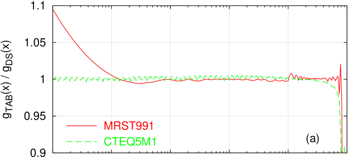
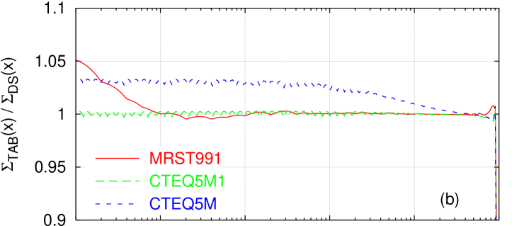
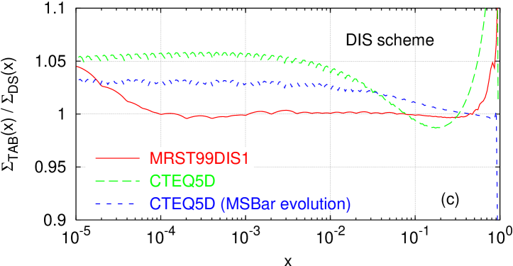
Figure 7: Comparisons between evolution encoded in two widely used tabulated global-fit PDF sets (TAB) [26, 24] and our evolution (DS). In all cases we start with the global-fit (tabulated, interpolated) distribution at $10$ GeV, evolve up to $179$ GeV and then compare to the tabulated distribution at the higher scale; (a) and (b) are in the $\overline{\mbox{\scriptsize MS}}$ scheme, while $(c)$ is for the DIS scheme.

As a test of our evolution code we decided to compare to the latest available tabulated evolution of the MRST [26], CTEQ [24] and GRV [25] groups. It was our expectation that following the work of the 1995/96 HERA workshop (see for example [47]), the latest available tabulated distributions would embody reasonably accurate evolution.

The comparisons indicate that our code is functioning properly since we generally agree with the evolution of at least one of the tabulated global-fit PDF sets. However in certain situations (probably of limited practical phenomenological relevance) we do see significant disagreement with one of MRST or CTEQ and in what follows we give a summary of our findings.

To carry out the comparison we adopted the following procedure. We started with the MRST or CTEQ tabulated (interpolated in $x$) distribution at $Q=10$ GeV and evolved it up to $179$ GeV with our evolution routines. We then took the ratio of the tabulated distribution at $179$ GeV and our evolved distribution. This is plotted for MRST and CTEQ in figure 7. We have chosen an upper limit of $179$ GeV rather than a ‘round number’ because it is a grid point of the MRST distributions: the interpolation provided with the MRST99 PDF sets is linear in $Q^{2}$ (as mentioned earlier) and a choice of $Q$ in between grid points introduces errors of the order of a couple of percent.

Figure 7a shows the results for the gluon distribution — there is good agreement with CTEQ and MRST over most of the range in $x$. However at small $x\lesssim 10^{-4}$ we find significant disagreement with MRST at a level of up to $10\%$, whereas the agreement with CTEQ remains perfect. At large $x\gtrsim 0.5$ there is slight disagreement with the CTEQ evolution, while agreement with MRST remains good up to $x\gtrsim 0.8$. It should be kept in mind that in this region the gluon distribution is in any case very small, and poorly constrained experimentally.

We note that the small irregularities of the curves arise because slight non-smoothness of the starting distributions (a consequence of the interpolation in $x$) gets amplified after convolutions with the plus-distributions of the splitting functions.

Figure 7b shows the analogous results for the quark singlet distribution,

$$\Sigma(x)\;=\sum_{j=u,d,s,\ldots}\left(q_{j}(x)+{\bar{q}}_{j}(x)\right).$$ (F.13)

The problem in the MRST distributions at small $x$ are present here too, though they are reduced by a factor of $2$. At large $x$ the agreement is uniformly good. We also show a comparison with the CTEQ5M evolution which uses some numerical approximations in the NLO evolution (see the note in the archive v3 of [24]), which is useful for reference below.

We have not explicitly shown comparisons with the GRV98 $\overline{\mbox{\scriptsize MS}}$ global-fit evolution [25] — there we find only small differences, generally less than $1\%$, which can be ascribed to a different convention for the treatment of higher-order terms in the evolution. Detailed comparisons with Vogt’s code, using the same convention for the higher-order terms, gives systematic agreement to a relative accuracy of better than $10^{-4}$ for $x<0.8$ [48].

We also wished to test our DIS scheme evolution, figure 7c. The DIS factorisation scheme is defined as the scheme in which all higher-order corrections to the $F_{2}$ coefficient functions are zero. Again we start with tabulated global-fit distributions (now in the DIS scheme) at $10$ GeV, evolve them up to $179$ GeV (with DIS scheme splitting functions) and compare with the tabulated distributions at the higher scale. Ignoring the small-$x$ problem, with MRST there is generally good agreement. There is a moderate discrepancy at large $x$, however we believe that this is because of the convention adopted by MRST to define the DIS scheme — all their fitting and evolution is done in the $\overline{\mbox{\scriptsize MS}}$ scheme, and then at each $Q$ value they calculate the DIS-scheme distribution from the $\overline{\mbox{\scriptsize MS}}$ distributions. This differs from straightforward DIS scheme evolution by NNL terms, which are largest at large $x$ because of a $\ln(1-x)/(1-x)_{+}$ enhancement.

With CTEQ, the agreement is quite poor and we identify two reasons for this. Firstly there is no updated version of the DIS scheme distributions (i.e. no equivalent to CTEQ5M1), so the numerical inaccuracies present in CTEQ5M (see figure 7b) are present in CTEQ5D as well. Secondly it seems that the NLO splitting functions used for the evolution are in the $\overline{\mbox{\scriptsize MS}}$ scheme: if we use $\overline{\mbox{\scriptsize MS}}$ splitting functions for the evolution then the resulting disagreement is identical to that due to numerical approximations that is to be seen in CTEQ5M.

We note that the DIS scheme was not examined in the context of the 1995/96 HERA workshop studies [47] and it would perhaps be worth performing a similar ‘standardisation exercise’ also in the DIS scheme.

References

-
[1]
S. Catani, L. Trentadue, G. Turnock and B. R. Webber,
Nucl. Phys. B 407 (1993) 3;
S. Catani, G. Turnock, B. R. Webber and L. Trentadue, Phys. Lett. B 263 (1991) 491. - [2] S. Catani, G. Turnock and B. R. Webber, Phys. Lett. B 295 (1992) 269.
-
[3]
S. Catani, Y. L. Dokshitzer, F. Fiorani and B. R. Webber,
Nucl. Phys. B 377 (1992) 445;
S. Catani, Y. L. Dokshitzer and B. R. Webber, Phys. Lett. B 322 (1994) 263;
S. J. Burby, Phys. Lett. B 453 (1999) 54 [hep-ph/9902305]. - [4] Y. L. Dokshitzer, A. Lucenti, G. Marchesini and G. P. Salam, JHEP 9801 (1998) 011 [hep-ph/9801324].
- [5] S. Catani and B. R. Webber, Phys. Lett. B 427 (1998) 377 [hep-ph/9801350]; S. Catani and B. R. Webber, JHEP 9710 (1997) 005 [hep-ph/9710333].
-
[6]
M. Acciarri et al. [L3 Collaboration],
Phys. Lett. B 489 (2000) 65
[hep-ex/0005045];
P. A. Movilla Fernandez, S. Bethke, O. Biebel and S. Kluth, hep-ex/0105059;
P. Abreu et al. [DELPHI Collaboration], Phys. Lett. B 456 (1999) 322;
ALEPH Collaboration, CERN-OPEN-99-337 Prepared for International Europhysics Conference on High-Energy Physics (HEP 97), Jerusalem, Israel, 19-26 Aug 1997;
The LEP QCD Working Group, “Preliminary Combination of Values Derived from Event Shape Variables at LEP,” ALEPH 01-038 Physic 01-012, DELPHI 2001-043 PHYS 893, L3 note 2661, OPAL TN689. -
[7]
S. Kluth, P. A. Movilla Fernandez, S. Bethke, C. Pahl and P. Pfeifenschneider,
Eur. Phys. J. C 21 (2001) 199
[hep-ex/0012044];
G. Dissertori, Nucl. Phys. Proc. Suppl. 65 (1998) 43 [hep-ex/9705016]. - [8] C. Adloff et al. [H1 Collaboration], Phys. Lett. B 406 (1997) 256 [hep-ex/9706002].
- [9] C. Adloff et al. [H1 Collaboration], Eur. Phys. J. C 14 (2000) 255 [Erratum-ibid. C 18 (2000) 417] [hep-ex/9912052].
-
[10]
G. J. McCance [for the H1 and ZEUS Collaborations],
hep-ex/0008009, talk given at the 35th Rencontres de Moriond: QCD and
High Energy Hadronic Interactions, France, March 2000;
H. Martyn [for the H1 and ZEUS Collaborations], hep-ex/0010046, talk given at 30th International Conference on High-Energy Physics (ICHEP 2000), Osaka, Japan, 27 Jul - 2 Aug 2000. - [11] V. Antonelli, M. Dasgupta and G. P. Salam, JHEP 0002 (2000) 001 [hep-ph/9912488].
- [12] M. Dasgupta and G. P. Salam, Phys. Lett. B 512 (2001) 323 [hep-ph/0104277].
- [13] M. Dasgupta and G. P. Salam, in preparation.
- [14] G. P. Salam and D. Wicke, JHEP 0105 (2001) 061 [hep-ph/0102343].
-
[15]
A. Banfi, G. Marchesini, Y. L. Dokshitzer and G. Zanderighi,
JHEP 0007 (2000) 002
[hep-ph/0004027];
A. Banfi, Y. L. Dokshitzer, G. Marchesini and G. Zanderighi, Phys. Lett. B 508 (2001) 269 [hep-ph/0010267]. A. Banfi, Y. L. Dokshitzer, G. Marchesini and G. Zanderighi, JHEP 0105 (2001) 040 [hep-ph/0104162]. A. Banfi, G. Marchesini, G. Smye and G. Zanderighi, JHEP 0108 (2001) 047 [hep-ph/0106278]. - [16] S. J. Burby and E. W. N. Glover, JHEP 0104 (2001) 029 [hep-ph/0101226].
- [17] S. Catani, M. L. Mangano, P. Nason and L. Trentadue, Nucl. Phys. B 478 (1996) 273 [hep-ph/9604351].
- [18] S. D. Ellis and W. J. Stirling, Phys. Rev. D 23 (1981) 214.
- [19] P. E. Rakow and B. R. Webber, Nucl. Phys. B 187 (1981) 254.
- [20] G. Parisi and R. Petronzio, Nucl. Phys. B 154 (1979) 427.
-
[21]
G. P. Korchemsky and G. Sterman,
Nucl. Phys. B437 (1995) 415
[hep-ph/9411211];
G. P. Korchemsky, G. Oderda and G. Sterman, presented at 5th International Workshop on Deep Inelastic Scattering and QCD (DIS 97), Chicago, IL, April 1997 hep-ph/9708346;
G. P. Korchemsky and G. Sterman, Nucl. Phys. B 555 (1999) 335 [hep-ph/9902341]. - [22] Y. L. Dokshitzer and B. R. Webber, Phys. Lett. B 404 (1997) 321 [hep-ph/9704298].
- [23] Y. L. Dokshitzer, G. Marchesini and G. P. Salam, Eur. Phys. J. directC 3 (1999) 1 [Erratum-ibid. C 1 (2001) 1] [hep-ph/9812487].
- [24] H. L. Lai et al. [CTEQ Collaboration], Eur. Phys. J. C 12 (2000) 375 [hep-ph/9903282]; see also http://www.phys.psu.edu/~cteq/CTEQ5Table/.
- [25] M. Gluck, E. Reya and A. Vogt, Eur. Phys. J. C 5 (1998) 461 [hep-ph/9806404]; see also http://durpdg.dur.ac.uk/hepdata/grv.html .
-
[26]
A. D. Martin, R. G. Roberts, W. J. Stirling and R. S. Thorne,
Eur. Phys. J. C 14 (2000) 133
[hep-ph/9907231];
see also http://durpdg.dur.ac.uk/hepdata/mrs.html -
[27]
S. Catani, B. R. Webber and G. Marchesini,
Nucl. Phys. B 349 (1991) 635;
Y. L. Dokshitzer, V. A. Khoze and S. I. Troian, Phys. Rev. D 53 (1996) 89 [hep-ph/9506425]. - [28] D. Graudenz, hep-ph/9710244.
- [29] A. Banfi, G. P. Salam and G. Zanderighi, in preparation.
- [30] E. Gardi and J. Rathsman, Nucl. Phys. B 609 (2001) 123 [hep-ph/0103217].
-
[31]
R. Akhoury and V. I. Zakharov,
Phys. Lett. B357 (1995) 646
[hep-ph/9504248].
R. Akhoury and V. I. Zakharov, Nucl. Phys. B465 (1996) 295 [hep-ph/9507253]. - [32] Y. L. Dokshitzer, A. Lucenti, G. Marchesini and G. P. Salam, JHEP 9805 (1998) 003 [hep-ph/9802381].
-
[33]
Y. L. Dokshitzer and B. R. Webber,
Phys. Lett. B352 (1995) 451
[hep-ph/9504219];
Y. L. Dokshitzer, G. Marchesini and B. R. Webber, Nucl. Phys. B469 (1996) 93 [hep-ph/9512336];
M. Dasgupta and B. R. Webber, Phys. Lett. B382 (1996) 273 [hep-ph/9604388]. - [34] Y. L. Dokshitzer, A. Lucenti, G. Marchesini and G. P. Salam, Nucl. Phys. B511 (1998) 396 [hep-ph/9707532], erratum ibid. B593 (2001) 729.
- [35] M. Dasgupta and B. R. Webber, JHEP 9810 (1998) 001 [hep-ph/9809247].
- [36] G. P. Salam and Z. Trócsányi, unpublished result.
- [37] S. Catani and M. H. Seymour, Phys. Lett. B 378 (1996) 287 [hep-ph/9602277]; S. Catani and M. H. Seymour, Nucl. Phys. B 485 (1997) 291 [hep-ph/9605323].
-
[38]
R. K. Ellis and S. Veseli,
Nucl. Phys. B 511 (1998) 649
[hep-ph/9706526];
A. Kulesza and W. J. Stirling, Eur. Phys. J. C 20 (2001) 349 [hep-ph/0103089]. - [39] A. D. Martin, R. G. Roberts, W. J. Stirling and R. S. Thorne, paper in preparation.
-
[40]
V. Berezinsky and M. Kachelriess,
Phys. Rev. D 63 (2001) 034007
[hep-ph/0009053];
S. Sarkar and R. Toldra, hep-ph/0108098. - [41] D. A. Kosower, Nucl. Phys. B 506 (1997) 439 [hep-ph/9706213].
- [42] M. A. J. Botje, Zeus Note 97–066, see http://www.nikhef.nl/ h24/qcdnum/.
- [43] P. Santorelli and E. Scrimieri, Phys. Lett. B 459 (1999) 599 [hep-ph/9807572].
- [44] C. Pascaud and F. Zomer, hep-ph/0104013.
- [45] P. G. Ratcliffe, Phys. Rev. D 63 (2001) 116004 [hep-ph/0012376].
- [46] See for example the section (18.3) on singular kernels in Numerical Recipes in Fortran 77: The Art of Scientific Computing, William H. Press, et al, Cambridge University Press (1992).
- [47] J. Blumlein, S. Riemersma, M. Botje, C. Pascaud, F. Zomer, W. L. van Neerven and A. Vogt, hep-ph/9609400.
- [48] G. P. Salam and A. Vogt, in preparation.