Abstract

We investigate corrections to the handbag approach for wide-angle Compton scattering off protons at moderately large momentum transfer: the photon-parton subprocess is calculated to next-to-leading order in $\alpha_{s}$ and contributions from the generalized parton distribution ${E}$ are taken into account. Photon and proton helicity flip amplitudes are non-zero due to these corrections which leads to a wealth of polarization phenomena in Compton scattering. Thus, for instance, the incoming photon asymmetry or the transverse polarization of the proton are non-zero although small.

PACS: 13.60.Hb, 13.88.+e, 14.20.Dh

1 Introduction

Probing the proton with high-energy photons provides information about its inner structure. The most famous process used for such investigations is deep inelastic lepton-proton scattering. From a dynamical point of view this process represents forward (virtual) Compton scattering and is described by the handbag diagram shown in Fig. 1. Recent theoretical developments revealed that the physics of the handbag diagram is also of importance for deeply virtual [1, 2] and wide-angle [3, 4] Compton scattering off protons. Both these processes refer to complementary kinematical situations. The region of deeply virtual scattering is characterized by small momentum transfer from the initial to the final proton and a large photon virtuality while in the wide-angle region the situation is reversed. As has been argued in [3, 4] the wide-angle Compton amplitudes approximately factorize into hard photon-parton subprocess amplitudes and proton matrix elements representing the soft emission and reabsorption of a parton by the proton. These matrix elements are moments of generalized parton distributions (GPDs) [1, 5, 6] and can be regarded as new form factors of the protons. The GPDs also encode the soft physics information required to describe deeply virtual Compton scattering. That the handbag diagram, i.e. elastic scattering of photons from quarks, controls Compton scattering has been conjectured by Bjorken and Paschos [7] and by Scott [8] long time ago as we note in passing.

It is however to be emphasized that the handbag contribution to wide-angle Compton scattering formally represents only a power correction to the leading-twist perturbative contribution [9]. This contribution for which all partons the proton is composed participate in the hard scattering and not only a single one as in the handbag, has been calculated several times [10] with partially contradicting results. According to the most recent study [11], it seems difficult to account for the wide-angle data on Compton scattering [12]. This result as well as similar observations made with the pion and the proton electromagnetic form factors [13, 14] have lead to the assumption of a dominant handbag contribution for momentum transfers below about 100 GeV². There is a third contribution to Compton scattering. It has the topology of the so called cat’s ears graphs where the hard subprocess involves two partons. It is reasonable to assume that the magnitude of this contribution is intermediate between the handbag and the perturbative one and that it can be neglected in the kinematical range of interest.

In this work we are going to investigate perturbative and non-perturbative QCD corrections to the handbag contribution for wide-angle Compton scattering. We calculate the next-to-leading order (NLO) corrections to the subprocess and, motivated by the surprising result for the Pauli form factor found at JLab [15], we study the bearing of the in [3, 4] neglected form factor $R_{T}$ on the predictions. We begin with a sketch of the handbag approach and the calculation of the NLO corrections (Sect. 2). A brief discussion of the model used for the form factors, or the underlying GPDs, follows (Sect. 3). Sect. 4 is devoted to a comprehensive discussion of the predictions for a large set of observables and their comparison with the results presented in [4] and with those obtained with other theoretical concepts. This may facilitate the interpretation of future experimental data on wide-angle Compton scattering that might be obtained at Spring-8, JLab or at an ELFE-type accelerator. Finally we discuss the possibility of measuring the Compton form factors (Sect. 5) and close with a summary (Sect. 6).

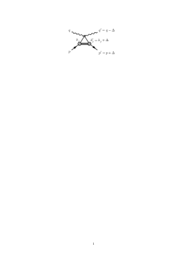
Figure 1: The handbag diagram for Compton scattering off protons. The horizontal lines represent any number of spectator partons.

2 The handbag contribution

Let us sketch the calculation of the handbag contribution to wide-angle Compton scattering; for details we refer to [4]. For Mandelstam variables, $s$, $t$ and $u$, that are large on a hadronic scale, $\Lambda^{2}$, of the order of 1 GeV², the Compton amplitudes are calculated from the handbag graph displayed in Fig. 1. Its contribution is defined through the assumption that the soft hadron wave functions occurring in the Fock decomposition of the proton, are dominated by parton virtualities in the range $|k_{i}^{2}|\raisebox{-4.0pt}{$\,\stackrel{{\scriptstyle\textstyle<}}{{\sim}}\,$}\Lambda^{2}$ and by intrinsic transverse parton momenta ${\bf k}_{\perp}{}_{i}$ that satisfy ${\bf k}_{\perp}{}_{i}^{2}/x_{i}\raisebox{-4.0pt}{$\,\stackrel{{\scriptstyle\textstyle<}}{{\sim}}\,$}\Lambda^{2}$. The intrinsic transverse momentum of a parton is defined in a frame where its parent’s hadron transverse momentum is zero; $x_{i}=k_{i}^{+}/p^{+}$ is the usual light-cone momentum fraction. It is of advantage to choose a symmetric frame of reference where the plus and minus light-cone components of the momentum transfer, $\Delta$, are zero (for the definition of the kinematics see Fig. 1). This implies $t=-{\bf\Delta}_{\perp}$ as well as a vanishing skewedness parameter, $\xi=(p-p^{\prime})^{+}/(p+p^{\prime})^{+}$. One can then show that the photon-parton scattering is hard and the momenta $k_{j}^{\phantom{.}}$, $k^{\prime}_{j}$ of the active partons, i.e. those to which the photons couple (see Fig. 1), are approximately on-shell, collinear with their parent hadrons and with momentum fractions $x_{j}^{\phantom{.}}=x^{\prime}_{j}=1$. This leads to an approximate equality of the Mandelstam variables in the photon-parton subprocess and in the overall photon-proton reaction up to corrections of order $\Lambda^{2}/t$.

In view of this the helicity amplitudes ${\cal M}_{\mu^{\prime}\nu^{\prime},\,\mu\nu}$ of wide-angle Compton scattering in the symmetric frame are given by

$${\cal M}_{\mu^{\prime}+,\,\mu+}(s,t) = \;2\pi\alpha_{\rm em}\left[{\cal H}_{\mu^{\prime}+,\,\mu+}(s,t)\,(R_{V}(t)+R_{A}(t))\,+\,{\cal H}_{\mu^{\prime}-,\,\mu-}(s,t)\,(R_{V}(t)-R_{A}(t))\right]\,,$$

$${\cal M}_{\mu^{\prime}-,\,\mu+}(s,t) = \;-\pi\alpha_{\rm em}\frac{\sqrt{-t}}{m}\left[{\cal H}_{\mu^{\prime}+,\,\mu+}(s,t)\,+\,{\cal H}_{\mu^{\prime}-,\,\mu-}(s,t)\,\right]\,R_{T}(t)\,.$$ (1)

Here, $\mu$ ($\nu$) and $\mu^{\prime}$ ($\nu^{\prime}$) denote the light-cone helicities [16, 17] of the incoming and outgoing photon (proton), respectively. $m$ is the proton mass. For the sake of legibility explicit helicities are labeled only by their signs. We emphasize that the proton helicity flip amplitudes have been neglected in Refs. [3, 4]. Below we will discuss under which circumstances this is reasonable and when not.

The soft proton matrix elements, $R_{i}$ ($i=V,A,T$), appearing in Eq. (1) represent new types of proton form factors. They are defined as $1/x$-moments of GPDs at zero skewedness. For active quarks of flavour $a$ ($u$, $d$, …) they read

$$R_{V}^{a}(t) = \int_{-1}^{1}\,\frac{d\bar{x}}{\bar{x}}\,H^{a}(\bar{x},0;t)\,,$$

$$R_{A}^{a}(t) = \int_{-1}^{1}\,\frac{d\bar{x}}{\bar{x}}\,{\rm sign}(\bar{x})\,\widetilde{H}^{a}(\bar{x},0;t)\,,$$

$$R_{T}^{a}(t) = \int_{-1}^{1}\,\frac{d\bar{x}}{\bar{x}}\,E^{a}(\bar{x},0;t)\,,$$ (2)

where $\bar{x}=(k_{j}+k_{j}^{\prime})^{+}/(p+p^{\prime})^{+}$. The full form factors in (1), specific to Compton scattering, are given by

$$R_{i}(t)=\sum_{a}e_{a}^{2}\,R_{i}^{a}(t)\,,$$ (3)

$e_{a}$ being the charge of quark $a$ in units of the positron charge. In principle there is a fourth form factor being related to the GPD $\widetilde{E}^{a}$ but it does not contribute to the Compton amplitudes in the symmetric frame. The form factors $R_{i}^{a}$ also appear in wide-angle photo- and electroproduction of mesons [18].

Last not least, the ${\cal H}_{\mu^{\prime}\lambda^{\prime},\,\mu\lambda}$ in Eq. (1) denote the $\gamma q\to\gamma q$ subprocess amplitudes where the helicities $\lambda$ and $\lambda^{\prime}$ refer to the quarks now. To leading order (LO) these amplitudes are to be calculated from the Feynman graphs shown in Fig. 2 a. One finds

$${\cal H}^{LO}_{++,++}=2\sqrt{\frac{s}{-u}}\,,\qquad{\cal H}^{LO}_{-+,-+}=2\sqrt{\frac{-u}{s}}\,,\qquad{\cal H}^{LO}_{-+,++}=0\,.$$ (4)

Since the quarks are taken as massless there is no quark helicity flip, ${\cal H}_{\mu^{\prime}\lambda,\,\mu-\lambda}=0$ to any order of $\alpha_{\rm s}$. Other helicity amplitudes are obtained from those given in (4) by parity and time reversal invariance

$${\cal H}_{-\mu^{\prime}-\lambda^{\prime},-\mu-\lambda}\,=\,{\cal H}_{\mu\lambda,\,\mu^{\prime}\lambda^{\prime}}\,=\,(-1)^{\mu-\lambda-\mu^{\prime}+\lambda^{\prime}}\,{\cal H}_{\mu^{\prime}\lambda^{\prime},\,\mu\lambda}\,.$$ (5)

Analogous relations hold for the ${\cal M}_{\mu^{\prime}\nu^{\prime},\,\mu\nu}$.

Figure 2: Feynman graphs for Compton scattering off on-shell quarks. a) is the LO graph, the others represent the NLO QCD corrections. Graphs with self energy corrections to external fermions and those with interchanged interaction points of the photons are not shown.

The NLO corrections to the $\gamma q\to\gamma q$ are to be calculated from the Feynman graphs b - e depicted in Fig. 2. We work in Feynman gauge and use dimensional regularization ($n=4+\epsilon$). As expected for the process at hand, the ultraviolet divergencies of the individual graphs cancel in the sum, the NLO amplitudes are ultraviolet safe. On the other hand, those photon helicity non-flip amplitudes which are non-zero at LO, are infrared (IR) divergent. They can be decomposed into an infrared divergent part $\propto{\cal H}^{LO}$ and an infrared safe one, ${\cal H}^{NLO}$,

$${\cal H}_{\mu+,\,\mu+}^{IR}=\frac{\alpha_{\rm s}}{4\pi}\,C_{F}\,C_{IR}(\mu_{F})\,{\cal H}_{\mu+,\,\mu+}^{LO}+{\cal H}_{\mu+,\,\mu+}^{NLO}\,,$$ (6)

where $C_{IR}$ embodies the IR singularities. $C_{F}$ ($=4/3$) is a colour factor and $\mu_{F}$ is a factorization scale being of order $\Lambda$. As usual, we interprete the infrared divergent pieces as non-perturbative physics and absorb them into the soft form factors. Thus, we write for any of the products of hard scattering amplitudes and form factors appearing in (1)

$${\cal H}_{\mu+,\,\mu+}(s,t)\,R_{i}(t) = \left[{\cal H}_{\mu+,\,\mu+}^{LO}\,\left(1+\frac{\alpha_{\rm s}}{4\pi}\,C_{F}\,C_{IR}(\mu_{F})\right)+{\cal H}_{\mu+,\,\mu+}^{NLO}\right]\,R_{i}(t)$$ (7)

$$= \left[{\cal H}_{\mu+,\,\mu+}^{LO}\,+{\cal H}_{\mu+,\,\mu+}^{NLO}\right]\,R_{i}(t,\mu_{F})\,+\,{\cal O}(\alpha_{\rm s}^{2})\,.$$

The next issue we are concerned with is the exact definition of $C_{IR}$. The infrared divergencies in (6) have the form

$$-\left(\frac{-t}{4\pi\mu_{F}^{2}}\right)^{\epsilon/2}\,\Gamma(1-\epsilon/2)\,(8/\epsilon^{2}-6/\epsilon)\,.$$ (8)

The $1/\epsilon^{2}$ term appears as a consequence of overlapping soft and collinear divergencies. The accompanying double logs become large at large $-t$ and have to be resummed together with corresponding higher order terms $[\alpha_{\rm s}\ln^{2}(-t/\mu_{F}^{2})]^{n}$ in a Sudakov factor [19]. The same problems occur in the Feynman contribution to the electromagnetic form factor of the proton which is the analogue of the handbag contribution to Compton scattering. To NLO the $\gamma^{*}\to q\bar{q}$ vertex appearing in that calculation, provides infrared singularities identically to (8) which have to be absorbed into the soft hadronic matrix element, too. It is, of course, natural to use the same scheme for the regularization of the IR divergencies for both the Feynman and the handbag contribution. Since customarily the Sudakov factor is considered as part of the electromagnetic form factor [19, 20], i.e. the latter already includes resummed double logs, we are forced to identify $C_{IR}$ with the full expression (8) in order to match with standard phenomenology and, in particular, with the model we employ in our numerical studies of Compton scattering. We remark in passing that the $\gamma^{*}\to q\bar{q}$ vertex also occurs in $e^{+}e^{-}\to q\bar{q}$. In this case the infrared singularities are compensated by real gluon emission. The infrared divergencies generated by the NLO QED corrections to Compton scattering off electrons cancel against those of double Compton scattering, $\gamma e\to\gamma\gamma e$ [21]. In deeply virtual Compton scattering only a single IR pole appears [22] but it can be shown that in the limit $x_{j}\to 1$ an additional singularity emerges [23].

After removal of the IR divergencies the NLO amplitudes read:

$${\cal H}_{++,++}^{NLO} = \frac{\alpha_{\rm s}}{2\pi}C_{F}\left\{\frac{\pi^{2}}{3}-7+\frac{2t-s}{s}\ln\frac{t}{u}\right.$$

$$\hskip 56.9055pt+\,\left.\ln^{2}\frac{-t}{s}+\frac{t^{2}}{s^{2}}\left(\ln^{2}\frac{t}{u}+\pi^{2}\right)-2i\pi\ln\frac{-t}{s}\right\}\sqrt{\frac{s}{-u}}\,,$$

$${\cal H}_{-+,-+}^{NLO} = \frac{\alpha_{\rm s}}{2\pi}C_{F}\left\{\frac{4}{3}\pi^{2}-7+\frac{2t-u}{u}\ln\frac{-t}{s}+\ln^{2}\frac{t}{u}\right.$$

$$\left.\hskip 56.9055pt+\,\frac{t^{2}}{u^{2}}\ln^{2}\frac{-t}{s}-2i\pi\left(\frac{2t-u}{2u}+\frac{t^{2}}{u^{2}}\ln\frac{-t}{s}\right)\right\}\sqrt{\frac{-u}{s}}\,,$$

$${\cal H}_{-+,++}^{NLO} = -\frac{\alpha_{\rm s}}{2\pi}C_{F}\left\{\sqrt{\frac{s}{-u}}+\sqrt{\frac{-u}{s}}\right\}\,.$$ (9)

Since in wide-angle Compton scattering $-t$ and $-u$ are of order $s$ there are no large logs in the NLO amplitudes. We also see that the NLO amplitudes possess both non-zero imaginary parts and non-zero photon helicity flips.

At the one-loop level, there is a complication which we have to discuss next, namely gluons have to be considered as active partons as well. The treatment of the gluonic contributions to wide-angle Compton scattering is analogous to that one utilized in wide-angle photo- and electroproduction of vector mesons [18]. The gluonic contributions factorize into the parton subprocess $\gamma g\to\gamma g$ and gluonic form factors. In contrast to the case of quarks, the partonic amplitudes now allow parton, i.e. gluon, helicity flips.

For gluon helicity non-flip the gluonic contributions have a representation analogous to (1). The corresponding form factors read

$$R_{V}^{g}(t)=\sum_{a}e^{2}_{a}\int_{0}^{1}\frac{d\bar{x}}{\bar{x}^{2}}\,H^{g}(\bar{x},0;t)\,,$$ (10)

and analogously for the other ones. The range of integration is restricted to the interval $[0,1]$ since gluons and antigluons are the same particles. The additional factor $1/\bar{x}$ is conventional; it appears as a consequence of the definition of the gluon GPDs [1, 5, 6] which implies the forward limits

$$\bar{x}g(\bar{x})=H^{g}(\bar{x},0;0)\,,\qquad\bar{x}\Delta g(\bar{x})=\widetilde{H}^{g}(\bar{x},0;0)\,.$$ (11)

With regard to this definition we still term (10) a $1/\bar{x}$-moment. The sum in (10) runs over the flavors $u$, $d$, $s$ which suffices for the range of energy we are interested in. For gluon helicity flip we do not present details here because these contributions are neglected in our numerical studies as those proportional to the form factors $R_{A}^{g}$ and $R_{T}^{g}$. This is justified since, as we will argue in Sec. 3, the gluon form factors are expected to be smaller than the corresponding quark ones at large $-t$ and since the gluonic contributions only appear to order $\alpha_{\rm s}$. Hence, we only consider the contribution $\propto R_{V}^{g}$. It reads

$$2\pi\alpha_{\rm em}\left[{\cal H}^{g}_{\mu^{\prime}+,\,\mu+}(s,t)+{\cal H}^{g}_{\mu^{\prime}-,\,\mu-}(s,t)\right]\,R_{V}^{g}(t)\,,$$ (12)

and is to be added to the proton helicity non-flip amplitudes ${\cal M}_{\mu^{\prime}+,\,\mu+}$ in (1).

Figure 3: Sample Feynman graphs for photon-gluon scattering.

The photon-gluon amplitudes are to be calculated from the three graphs shown in Fig. 3. There are three further graphs contributing to order $\alpha_{\rm s}$ which however reduce to first three ones by reversing the fermion number flow. After some algebra we find for the gluon helicity non-flip amplitudes

$${\cal H}^{g}_{++,++} = \frac{\alpha_{s}}{\pi}\left\{\frac{t^{2}+u^{2}}{2s^{2}}\left(\ln^{2}\frac{t}{u}+\pi^{2}\right)+\frac{t-u}{s}\ln\frac{t}{u}+1\right\}\,,$$

$${\cal H}^{g}_{-+,-+} = \frac{\alpha_{s}}{\pi}\left\{\frac{s^{2}+t^{2}}{2u^{2}}\ln^{2}\frac{-t}{s}+\frac{t-s}{u}\ln\frac{-t}{s}+1-i\pi\left(\frac{t-s}{u}+\frac{s^{2}+t^{2}}{u^{2}}\ln\frac{-t}{s}\right)\right\}\,,$$

$${\cal H}^{g}_{-+,++} = -\frac{\alpha_{s}}{\pi}\,.$$ (13)

Except for a different normalization these amplitudes agree with those given in Ref. [24]. In this recent paper the gluon helicity flip amplitudes can be found, too.

3 Modelling the GPDs

In order to predict wide-angle Compton scattering a model for the GPDs at large $-t$ and zero skewedness is required. In Ref. [25] (see also [4, 26]) it has been shown on the basis of light-cone quantization that the GPDs possess a representation in terms of light-cone wave function overlaps. This representation allows the construction of a simple model for the GPDs by parameterizing the transverse momentum dependence of a $N$-particle wave function as

$$\Psi_{N}\propto\exp{\left[-a_{N}^{2}\sum_{i=1}^{N}k_{\perp i}^{2}/x_{i}\right]}\,,$$ (14)

which is in line with the central assumption of the handbag approach of restricted $k_{\perp i}^{2}/x_{i}$, necessary to achieve factorization of the amplitudes into soft and hard parts. Without explicit specification of the $x$-dependencies of the wave functions one can then calculate the $\xi=0$ GPDs from the overlap representation if a common transverse size parameter $a=a_{N}$ is used. This ansatz leads to

$$H^{a}(\bar{x},0;t)=\exp{\left[a^{2}t\frac{1-\bar{x}}{2\bar{x}}\right]}\,q_{a}(\bar{x})\,,\qquad\widetilde{H}^{a}(\bar{x},0;t)=\exp{\left[a^{2}t\frac{1-\bar{x}}{2\bar{x}}\right]}\,\Delta q_{a}(\bar{x})\,,$$ (15)

where $q_{a}$ and $\Delta q_{a}$ are the ordinary unpolarized and polarized parton distributions for a quark of flavour $a$, respectively. An analogous representation holds for the gluon GPDs with the replacement of $q_{a}$ and $\Delta q_{a}$ by $\bar{x}g$ and $\bar{x}\Delta g$, respectively.

Taking the parton distributions from one of the current analyses of deep inelastic lepton-nucleon scattering, e.g. from Ref. [27], and using a value of $\simeq 1{\rm GeV}^{-1}$ for the transverse size parameter $a$, one obtains acceptable results for the unpolarized Compton cross section as well as for the proton and neutron electromagnetic Dirac form factors, $F_{1}$, which represent $x^{0}$-moments of $H^{a}$. The model GPDs (15) have been improved somewhat by treating the lowest three proton Fock states explicitly with specified wave functions [4, 14] whose parameters are fitted to data for the electromagnetic form factors and to the parton distributions given in [27]. Due to this procedure the form factors effectively include the Sudakov factors and do practically not depend on the factorization scale. Since we are merely interested in a restricted range of momentum transfer we ignore the evolution of the GPDs as has been done in previous work [3, 4, 18]. As shown by Vogt [28], the evolution can be incorporated in the overlap model for the GPDs at the expense of a scale dependent transverse size parameter. Numerical results for the form factors, obtained from the improved version of the overlap model [4, 18], are displayed in Fig. 4. We will employ these results in our numerical studies.

Figure 4: The Compton form factors $R_{V}$, $R_{A}$ and $R_{V}^{g}$, scaled by $t^{2}$, vs. $-t$.

Let us now discuss the form factor $R_{T}$. The overlap representation of the underlying GPD $E^{a}$ involves components of the proton wave functions where the parton helicities do not add up to the helicity of the proton. In other words, parton configurations with non-zero orbital angular momentum contribute to it. That $E^{a}$ involves parton orbital angular momentum in an essential way is also reflected in Ji’s angular momentum sum rule [29]. Whereas $R_{V}$ and $F_{1}$ represent different moments of the GPD $H^{a}$, correspond $R_{T}$ and the Pauli form factor, $F_{2}$, to $E^{a}$. Since, at large $-t$, the integrals (2) for $R_{V}$ and $R_{T}$ as well as those for their electromagnetic counter parts, $F_{1}$ and $F_{2}$, are dominated by the region $\bar{x}\to 1$ where the valence $u$-quarks provide most of the contributions, there is little difference between $1/x$ and $x^{0}$-moments. This is sufficiently suggestive to assume that

$$R_{T}/R_{V}\simeq F_{2}/F_{1}\,.$$ (16)

Inspection of the SLAC data on $F_{2}$ [30] therefore leads one to the expectation $R_{T}/R_{V}\propto\Lambda^{2}/t$ with the consequence of parameterically suppressed ($\propto\Lambda/\sqrt{-t}$) contributions from $R_{T}$ to the Compton amplitudes (1). Given that already the evaluation of the handbag diagram is only accurate up to corrections of order $\Lambda^{2}/t$, $R_{T}$ and consequently proton helicity flip is to be neglected for consistency. This has been done in previous LO calculations [3, 4]. However, the recent JLab measurement of $F_{2}$ [15] seems to indicate a behaviour $\propto\Lambda/\sqrt{-t}$ for the ratio of form factors rather than $\Lambda^{2}/t$. Provided this behaviour will be confirmed, $R_{T}$ cannot be omitted in the handbag approach; it contributes to the same order in $\Lambda/\sqrt{-t}$ as the other form factors, see (1). The results for Compton scattering presented in [3, 4] have to be revised accordingly. Note that a behaviour $\propto\Lambda/\sqrt{-t}$ for the ratio of form factors appears quite natural in the overlap representation [25, 31].

In the next section we will present predictions for Compton scattering using both the scenarios $R_{T}$ omitted and $R_{T}/R_{V}\propto\Lambda/\sqrt{-t}$ for comparison. In the latter case we use a value of 0.37 for the ratio

$$\kappa=\frac{\sqrt{-t}}{2m}\,\frac{R_{T}}{R_{V}}\,,$$ (17)

as taken from the experimental ratio of $F_{2}$ and $F_{1}$ measured by the JLab Hall A Collaboration [15]. In general $\kappa$ is a function of $t$.

The gluonic form factors play a minor role in our analysis since they contribute only to order $\alpha_{\rm s}$. Moreover, they are smaller than their quark counterparts at large $-t$ since there, as we argued above, the form factors are controlled by the region $\bar{x}\simeq 1$ where the valence $u$-quark dominates. $R_{T}^{g}$, related to $E^{g}$, as well as the gluon helicity flip form factors [17] involve parton orbital angular momentum. One may therefore anticipate that these form factors are smaller than $R_{V}^{g}$. $R_{A}^{g}$, being related to $\Delta g$, is expected to be very small, too [18]. Thus, only the largest of the gluonic form factors, $R_{V}^{g}$, is taken into account by us, the other ones are neglected. Numerical results for $R_{V}^{g}$ are taken from [18] and shown in Fig. 4.

4 Observables for Compton scattering off protons

The derivation of the Compton amplitudes within the handbag approach naturally requires the use of the light-cone helicity basis. However, for comparison with experimental and other theoretical results the use of the ordinary photon-proton c.m.s. helicity basis is more convenient. The c.m.s. helicity amplitudes $\Phi_{\mu^{\prime}\nu^{\prime},\,\mu\nu}$ (we keep the notation of the helicity labels) are obtained from the light-cone helicity amplitudes (1), defined in the symmetric frame, by the following transform [17]

$$\Phi_{\mu^{\prime}\nu^{\prime},\,\mu\nu}\,=\,{\cal M}_{\mu^{\prime}\nu^{\prime},\,\mu\nu}+\beta/2\left[\,(-1)^{1/2-\nu^{\prime}}{\cal M}_{\mu^{\prime}-\nu^{\prime},\,\mu\nu}+(-1)^{1/2+\nu}{\cal M}_{\mu^{\prime}\nu^{\prime},\,\mu-\nu}\,\right]+{\cal O}(\Lambda^{2}/t)\,,$$ (18)

where

$$\beta=\frac{2m}{\sqrt{s}}\,\frac{\sqrt{-t}}{\sqrt{s}+\sqrt{-u}}\,.$$ (19)

For convenience we will use below a more generic notation for the six independent helicity amplitudes [32]

$$\Phi_{1} = \Phi_{++++}\,,\qquad\Phi_{3}=\Phi_{-+++}\,,\qquad\Phi_{5}=\Phi_{+-+-}\,,$$

$$\Phi_{2} = \Phi_{--++}\,,\qquad\Phi_{4}=\Phi_{+-++}\,,\qquad\Phi_{6}=\Phi_{-++-}\,.$$ (20)

Inspection of (18) and (1) reveals that

$$\Phi_{2}=-\Phi_{6}\,+\,{\cal O}(\Lambda^{2}/t)\,,$$ (21)

within the handbag approach. The amplitudes $\Phi_{2}$, $\Phi_{3}$ and $\Phi_{6}$ are of order $\alpha_{\rm s}$.

In our numerical studies we choose $s/2$ as the scale of $\alpha_{\rm s}$ which is the typical virtuality one encounters in the Feynman graphs shown in Figs. 2 and 3, and evaluate $\alpha_{\rm s}$ from the two-loop expression for $n_{f}=4$ flavours and $\Lambda_{\overline{MS}}^{(4)}=305\,{\rm MeV}$ [33]. We emphasize that our predictions, termed scenario A in the following, include corrections of order $\alpha_{\rm s}$ and $\beta$ ($\propto\Lambda/\sqrt{-t}$) as well as contributions from $R_{T}$ (with $\kappa=0.37$). Terms of order $\alpha_{\rm s}^{2}$ and $\beta^{2}$ are neglected throughout. Thus, for instance, a square of a helicity amplitude is evaluated as

$$|{\cal H}|^{2}=|{\cal H}^{LO}|^{2}+2\,{\cal H}^{LO}\,{\rm Re}\,{\cal H}^{NLO}\,.$$ (22)

For comparison we also show the results given in [4] where only the LO subprocess amplitudes are taken into account and $R_{T}$ as well as the order $\Lambda/\sqrt{-t}$ corrections are omitted (scenario B).

Figure 5: Predictions from scenario A for the Compton cross section, scaled by $s^{6}$, versus $\cos\theta$ for various photon energies, $E$, in the laboratory frame. $\theta$ is the c.m.s. scattering angle. Data taken from Ref. [12]; they are only shown for $-t,-u\geq 2.5\;{\rm GeV}^{2}$ as a minimum condition for our approximations to be applicable.

The simplest but most important observable is the unpolarized cross section. In terms of the c.m.s. helicity amplitudes and within the handbag approach it reads:

$$\frac{d\sigma}{dt} = \frac{1}{32\pi(s-m^{2})^{2}}\left[|\Phi_{1}|^{2}+|\Phi_{2}|^{2}+2|\Phi_{3}|^{2}+2|\Phi_{4}|^{2}+|\Phi_{5}|^{2}+|\Phi_{6}|^{2}\right]$$ (23)

$$= \frac{\pi\alpha_{\rm em}^{2}}{4(s-m^{2})^{2}}\bigg{\{}R_{V}^{2}\,\big{[}1+\kappa^{2}\big{]}\big{|}{\cal H}_{++++}+{\cal H}_{+-+-}\big{|}^{2}+R_{A}^{2}\,\big{|}{\cal H}_{++++}-{\cal H}_{+-+-}\big{|}^{2}$$

$$\hskip 56.9055pt+2\,({\cal H}_{++++}^{LO}+{\cal H}_{+-+-}^{LO})\,{\rm Re}\,({\cal H}_{++++}^{g}+{\cal H}_{+-+-}^{g})\,R_{V}R_{V}^{g}\bigg{\}}\,,$$

where we keep the proton mass in the phase space factor. In Fig. 5 we compare our scenario A results for the Compton cross section, scaled by $s^{6}$, with experiment [12]. This scaling accounts for most of the energy dependence in the kinematical range of interest. As can be seen from Fig. 4, the form factors behave as $1/t^{2}$ in the momentum transfer range from about 5 to 15 GeV² and, consequently, the Compton cross section exhibits approximate dimensional counting rule behaviour ($\propto s^{-6}$) at fixed scattering angle in a limited range of energy. With increasing $-t$ the form factors gradually turn into a $\propto t^{-4}$ behaviour. In that region of $t$, likely well above $100\,{\rm GeV}^{2}$ as is argued in [4], the perturbative contribution to Compton scattering will take the lead. For our form factor model the contribution from $R_{T}$ results in a constant factor of 1.13 multiplying $R_{V}^{2}$ while that from $R_{A}$ is very small in the forward hemisphere and grows to about $17\%$ for $\cos\theta\simeq-0.6$. This comes about because $|{\cal H}_{++++}+{\cal H}_{+-+-}|^{2}\gg|{\cal H}_{++++}-{\cal H}_{+-+-}|^{2}$ in the wide angle region and because, according to the overlap model, $R_{V}>R_{A}$. In order to demonstrate the importance of the NLO corrections we display ratios of the NLO corrections for quarks and gluons and the LO result in Fig. 6. As can be seen from that figure the gluonic contribution amounts to less than $10\%$ in the entire $\cos\theta$ range of interest. The NLO corrections from quarks are small in the backward hemisphere while the grow up to about $30\%$ for $\cos\theta\to 1$. This happens because $s$ and $-t$ differ greatly for $\cos\theta\to 0.6$ and, hence, some of the logs in (9) become large. $\cos\theta\simeq 0.6$ is the border line for the applicability of the handbag approach beyond which $-t$ can hardly be regarded as being of order $s$.

Figure 6: Comparison between the NLO and LO results for the Compton cross section (contribution from $R_{T}$ not included) at a photon lab. energy of 6 GeV.

Given the quality of the data, and the small energies and low values of $-t$ and $-u$ at which they are available, the predictions following from the handbag approach are in fair agreement with experiment. Better data are clearly needed for a severe test of the handbag approach and its confrontation with other approaches. Cross sections of comparable magnitude have been obtained within a diquark model [34]. This model is a variant of the perturbative approach in which diquarks are considered as quasi-elementary constituents of the proton [35]. In the leading-twist perturbative approach, on the other hand, it seems difficult to account for the Compton data even if strongly asymmetric distribution amplitudes are used [11]. For more symmetric ones, like the asymptotic one or that one proposed in [14] the perturbative predictions are way below experiment [11].

Before we turn to the discussion of spin dependent observables a remark concerning the definition of the proton polarization states is in order. We use the convention advocated by Bourrely, Leader and Soffer [36] and define the rotation of a vector through an azimuthal angle $\varphi$ and a polar angle $\theta$ by the matrix $R(\varphi,\theta,0)$. We consider three different polarization states of the proton – $L$, $S$ and $N$ – defined as spin eigenstates of ${\bf A}\cdot{\bf\sigma}$ where ${\bf\sigma}$ is the vector formed of the Pauli matrices and ${\bf A}$ any of the unit vectors

$${\bf L}^{(}{}^{\prime)}=\frac{{\bf p}^{(}{}^{\prime)}}{|{\bf p}^{(}{}^{\prime)}|}\,,\qquad{\bf N}={\bf L}\times{\bf L}^{\prime}\,,\qquad{\bf S}^{(}{}^{\prime)}={\bf N}\times{\bf L}^{(}{}^{\prime)}\,.$$ (24)

${\bf p}$ and ${\bf p}^{\prime}$ denote the three-momenta of the incoming and outgoing protons, respectively. For Compton scattering a number of polarization observables have been introduced in order to probe theoretical ideas [32], many more can be defined in principle. Obviously, only a few of them can be discussed here.

One set of polarization observables are the two-spin correlations of which the helicity ($L$-type) correlations are of particular interest. That one of the photon and the proton in the initial state is defined by

$$A_{LL}\frac{d\sigma}{dt} = \frac{1}{2}\left[\frac{d\sigma(++)}{dt}-\frac{d\sigma(+-)}{dt}\right]$$ (25)

$$= \frac{1}{32\pi(s-m^{2})^{2}}\left[|\Phi_{1}|^{2}+|\Phi_{2}|^{2}-|\Phi_{5}|^{2}-|\Phi_{6}|^{2}\right]$$

$$= \frac{\pi\alpha_{\rm em}^{2}}{2(s-m^{2})^{2}}R_{A}\,\bigg{\{}R_{V}\,\Big{[}1-\beta\kappa\Big{]}\,\Big{[}\big{|}{\cal H}_{++++}\big{|}^{2}-\big{|}{\cal H}_{+-+-}\big{|}^{2}\Big{]}$$

$$\hskip 14.22636pt+\;R_{V}^{g}\,\big{(}{\cal H}_{++++}^{LO}-{\cal H}_{+-+-}^{LO}\big{)}\,{\rm Re}\,\big{(}{\cal H}_{++++}^{g}+{\cal H}_{+-+-}^{g}\big{)}\,\bigg{\}}\,.$$

Using the model form factors discussed in Sect. 3, we evaluate the initial state helicity correlation $A_{LL}$ for scenario A and compare it in Fig. 7 to that obtained from scenario B [4]. The $\cos\theta$ dependence of $A_{LL}$ approximately reflects that of the corresponding helicity correlation for the photon-parton subprocess, $(s^{2}-u^{2})/(s^{2}+u^{2})$, its size being however diluted by the form factors. We observe from Fig. 7 that the inclusion of $R_{T}$ and the NLO corrections reduce the values of $A_{LL}$ by about $0.1$ to $0.2$ as compared to the results from scenario B. The results from the handbag approach are opposite in sign to the diquark model predictions [34]. In the leading-twist perturbative approach, the results for $A_{LL}$ are also markedly different from our ones [11]. They are very sensitive to the proton distribution amplitudes used in the evaluation.

Figure 7: Predictions for the initial state helicity correlation $A_{\rm LL}$ from scenario A and B at photon lab. energies of 6 GeV and 12 GeV.

The analogous correlation between the helicities of the incoming photon and the outgoing proton is defined by

$$K_{LL}\frac{d\sigma}{dt} = \frac{d\sigma(++)}{dt}-\frac{d\sigma(+-)}{dt}$$ (26)

$$= \frac{1}{32\pi(s-m^{2})^{2}}\left[|\Phi_{1}|^{2}-|\Phi_{2}|^{2}-|\Phi_{5}|^{2}+|\Phi_{6}|^{2}\right]\,.$$

Since $\Phi_{2}=-\Phi_{6}$ in the handbag approach, see (21), we obtain

$$K_{LL}=A_{LL}\,.$$ (27)

The helicity transfer from the incoming to the outgoing photon reads

$$D_{LL}\frac{d\sigma}{dt} = \frac{d\sigma(++)}{dt}-\frac{d\sigma(+-)}{dt}$$ (28)

$$= \frac{1}{32\pi(s-m^{2})^{2}}\left[|\Phi_{1}|^{2}-|\Phi_{2}|^{2}-2|\Phi_{3}|^{2}+2|\Phi_{4}|^{2}+|\Phi_{5}|^{2}-|\Phi_{6}|^{2}\right]\,.$$

Although the photon helicity is not strictly conserved to NLO, the helicity transfer is

$$D_{LL}=1+{\cal O}(\alpha_{\rm s}^{2})\,,$$ (29)

as is evident from a comparison of (23) and (28).

One may also consider sideway proton spin directions, see (24). The correlation between the helicity of the incoming photon and the sideway ($S$-type) polarization of the incoming proton, parallel ($\rightarrow$) or antiparallel ($\leftarrow$) to the $S$-direction reads

$$A_{LS}\frac{d\sigma}{dt} = \frac{1}{2}\left[\frac{d\sigma(+\rightarrow)}{dt}-\frac{d\sigma(-\rightarrow)}{dt}\right]$$ (30)

$$= \frac{1}{16\pi(s-m^{2})^{2}}\,{\rm Re}\,\left[\,(\Phi_{1}-\Phi_{5})\Phi_{4}^{*}-(\Phi_{2}+\Phi_{6})\Phi_{3}^{*}\,\right]$$

$$= -\frac{\pi\alpha_{\rm em}^{2}}{2(s-m^{2})^{2}}\,R_{A}\,\bigg{\{}\frac{\sqrt{-t}}{2m}\,R_{T}\,\Big{[}1+\beta\kappa^{-1}\Big{]}\,\Big{[}\big{|}{\cal H}_{++++}\big{|}^{2}-\big{|}{\cal H}_{+-+-}\big{|}^{2}\Big{]}$$

$$+\quad\beta\,R_{V}^{g}\,\big{(}{\cal H}_{++++}^{LO}-{\cal H}_{+-+-}^{LO}\big{)}\,{\rm Re}\,\big{(}{\cal H}_{++++}^{g}+{\cal H}_{+-+-}^{g}\big{)}\bigg{\}}\,.$$

Predictions from scenario A are shown in Fig. 8, those obtained from scenario B are zero. $A_{LS}$ turns out to be rather independent of the photon energies. It is important to note that $A_{LS}$ is a observable that is very sensitive to the form factor $R_{T}$. The corrections from the term $\beta\kappa^{-1}$ are, however, substantial, in particular for the energies available at JLab; they cannot be ignored. This, after all, is the reason why, in contrast to [3, 4], we keep these terms. Neither in the diquark model [34] nor in the leading-twist perturbative approach [11] this observable has been discussed.

Figure 8: The correlation $A_{LS}$ at photon lab. energies of 6 GeV and 12 GeV.

The correlation between the helicity of the incoming photon and the sideway polarization of the outgoing proton is defined as

$$K_{LS}\frac{d\sigma}{dt} = \frac{d\sigma(+\rightarrow)}{dt}-\frac{d\sigma(-\rightarrow)}{dt}$$ (31)

$$= -\frac{1}{16\pi(s-m^{2})^{2}}\,{\rm Re}\,\left[\,(\Phi_{1}-\Phi_{5})\Phi_{4}^{*}+(\Phi_{2}+\Phi_{6})\Phi_{3}^{*}\,\right]\,.$$

Because of $\Phi_{2}=-\Phi_{6}$ it follows that

$$K_{LS}=-A_{LS}\,.$$ (32)

Correlations between the helicity of the incoming photon and the transverse ($N$-type) polarization of either the incoming or the outgoing proton are zero due to parity invariance

$$K_{LN}=A_{LN}=0\,.$$ (33)

A single-spin observable for Compton scattering is the incoming photon asymmetry $\Sigma$ which is defined as

$$\Sigma\frac{d\sigma}{dt} = \frac{1}{2}\left[\frac{d\sigma_{\perp}}{dt}-\frac{d\sigma_{\parallel}}{dt}\right]$$ (34)

$$= \frac{1}{16\pi(s-m^{2})^{2}}\,{\rm Re}\,\left[\,(\Phi_{1}+\Phi_{5})\Phi_{3}^{*}+(\Phi_{2}-\Phi_{6})\Phi_{4}^{*}\,\right]$$

$$= \frac{\alpha_{\rm s}\,\alpha_{\rm em}^{2}}{(s-m^{2})^{2}}\,\frac{(s-u)^{2}}{us}\,\Big{[}C_{F}\,R_{V}^{2}\,(1+\kappa^{2})+2\frac{\sqrt{-us}}{s-u}R_{V}R_{V}^{g}\Big{]}\,,$$

where $\perp$ and $\parallel$ refer to linear photon polarization normal to and in the scattering plane, respectively. Obviously, $\Sigma$ is zero to LO since there is no photon helicity flip. The predictions obtained from scenario A are shown in Fig. 9. $\Sigma$ is negative and small in absolute value. Approximately, i.e. if the terms $\propto R_{A}$ and $\propto R_{V}^{g}$ are neglected in (23), it is given by

$$\Sigma\simeq-\alpha_{\rm s}C_{F}/\pi\,.$$ (35)

Hence, the incoming photon asymmetry is nearly independent of the Compton form factors. In the diquark model [34] $\Sigma$ is negative too but smaller in absolute value. The leading-twist approach [11], on the other hand, provides rather large positive values for $\Sigma$.

Figure 9: The incoming photon asymmetry $\Sigma$ at photon lab. energies of 6 GeV and 12 GeV.

Last not least we want to comment on the ($N$-type) polarization or, as occasionally termed, the single spin asymmetry of the incoming proton, that of the outgoing one is analogous. The polarization of the incoming proton is defined by

$$P\frac{d\sigma}{dt} = \frac{1}{2}\left[\frac{d\sigma(\uparrow)}{dt}-\frac{d\sigma(\downarrow)}{dt}\right]$$ (36)

$$= \frac{1}{16\pi(s-m^{2})^{2}}\,{\rm Im}\,\left[\,(\Phi_{1}+\Phi_{5})\Phi_{4}^{*}-(\Phi_{2}-\Phi_{6})\Phi_{3}^{*}\,\right]\,,$$

where $\uparrow$ and $\downarrow$ denote the proton polarization parallel and antiparallel to the $N$-direction, respectively. The calculation of that polarization is a notoriously difficult task within QCD. Therefore, many experimentally observed polarization effects, as for instance the polarization in proton-proton elastic scattering at large momenta transfer [37], remained unexplained. As is well-known a non-zero polarization requires proton helicity flip and phase differences between the various helicity amplitudes. Both the necessary ingredients are provided by the handbag approach, helicity flips from $R_{T}$ and phases from the NLO corrections and we approximately obtain

$$P\simeq-\frac{\sqrt{-t}}{2m}\,\frac{R_{T}\,R_{V}^{g}}{R_{V}^{2}}\,\frac{\sqrt{-us}}{s-u}\,{\rm Im}\,\big{(}{\cal H}_{++++}^{g}+{\cal H}_{+-+-}^{g}\big{)}\,.$$ (37)

The polarization is of order $\alpha_{\rm s}$ and proportional to the gluonic contribution. Numerically it is very small, less than $3\%$ for our model form factors. The predictions for $P$ are to be taken with a grain of salt. The neglect of gluon helicity flip as well as $\alpha_{\rm s}^{2}$ and $\Lambda^{2}/t$ terms may lead to substantial corrections. Thus, at a conservative estimate, we can only say that an experimentally observed polarization larger in absolute value than, say, 0.1 - 0.2 near $\theta=90^{\circ}$ would be difficult to understand in the handbag approach.

5 Measuring the Compton form factors

In the preceding sections we presented predicitions for various observables of wide-angle Compton scattering within the handbag approach, using a model for the form factors that is based on light-cone wave function overlaps [4, 25]. On the other hand, a model-independent test of the handbag approach is provided by a measurement of the Compton form factors which can be performed through an analysis of the data for a set of observables to be at disposal for several values of $s$ and $t$. The crucial question is whether or not the experimentally determined form factors are independent of $s$ within the experimental and theoretical uncertainties.

At JLab the E99-114 collaboration plans to measure along with the differential cross section the two-spin correlations $K_{LL}$ and $K_{LS}$ [38]. Provided the quality of this data will be sufficiently good one may isolate the three form factors $R_{V}(t)$, $R_{A}(t)$ and $R_{T}(t)$ (or $\kappa(t)$) from it. As a first step towards a model-independent analysis, one may neglect the gluonic contributions everywhere and the term $\propto R_{A}$ in the cross section which, as we discussed above, is small. To the extend that these simplifications are justified, one finds

$$\frac{d\sigma}{dt} \simeq \frac{\pi\alpha_{\rm em}^{2}}{4(s-m^{2})^{2}}\,R_{V}^{2}(t)[1+\kappa^{2}(t)]\,\big{|}{\cal H}_{++++}+{\cal H}_{+-+-}\big{|}^{2}\,,$$

$$K_{LL} \simeq 2\,\frac{R_{A}(t)}{R_{V}(t)}\,\frac{1-\beta\kappa(t)}{1+\kappa^{2}(t)}\,\frac{\big{|}{\cal H}_{++++}\big{|}^{2}-\big{|}{\cal H}_{+-+-}\big{|}^{2}}{\big{|}\;{\cal H}_{++++}+{\cal H}_{+-+-}\;\big{|}^{2}}\,,$$

$$\frac{K_{LS}}{K_{LL}} \simeq \kappa(t)\,\frac{1+\beta\kappa^{-1}(t)}{1-\beta\kappa(t)}\,.$$ (38)

The cross section is essentially controlled by the form factor $R_{V}$ with, probably, only a small correction from $\kappa$. $K_{LL}$ measures the ratio $R_{A}/R_{V}$ with, however, substantial corrections from $\kappa$. The ratio $K_{LS}/K_{LL}$ determines the Compton analogue $R_{T}/R_{V}$ ($\propto\kappa$) to the ratio of the electromagnetic form factors $F_{2}$ and $F_{1}$. For large energies and scattering angles near $90^{\circ}$, the $\beta$ terms are negligible small and the analysis is markedly simplified. In Tab. 1 we present an assessment of the quality of the approximations (38). The discrepancies between (38) and the full results from scenario A do not exceed $15\%$ at a photon energy of 6 GeV. The use of the LO amplitudes in (38) instead of the full ones enlarges the discrepancies, in particular in the forward hemisphere, see Fig. 6. The form factors measured through (38) may be improved iteratively.

[$\cos\theta$	$\Delta(d\sigma/dt)$ [$\%$]	$\Delta(K_{LL})$ [$\%$]	$\Delta(K_{LS}/K_{LL})$ [$\%$]
- 0.6	1-6.2	-15.0	11.4
- 0	1-5.6	-12.4	12.2
-0.6	-14.8	-11.2	14.6

Table 1: The discrepancies between the approximations (38) and the full results from scenario A in percent of the full results at a photon lab. energy of 6 GeV.

6 Summary

As a complement to [4] we have calculated the NLO QCD corrections to the subprocess amplitudes and include the form factor $R_{T}$, related to the GPD ${E}$, in the analysis of wide-angle Compton scattering off protons. We have also considered the difference between the light-cone helicity basis in which the handbag graph is calculated, and the usual c.m.s. helicity one. Predictions for various Compton observables are given and compared to the leading contribution discussed in [4]. It turns out that these corrections are non-negligible in general although not unreasonably large. The NLO corrections and those due to the change of the helicity basis decrease with increasing energy while those due to the form factor $R_{T}$ keep their size provided $\kappa$ is independent of $t$. We stress that there are uncontrolled corrections of order $\Lambda^{2}/t$ in the handbag approach. For energies as low as, say, 3 GeV these corrections may be substantial. Our study may be of importance for severe tests of the handbag approach with future high-quality data for wide-angle Compton scattering which might be obtained at Spring-8, JLab or an ELFE-type accelerator.

References

- [1] A. V. Radyushkin, Phys. Rev. D56 5524 (1997) [hep-ph/9704207].
- [2] X. Ji and J. Osborne, Phys. Rev. D 58, 094018 (1998) [hep-ph/9801260]; J. C. Collins and A. Freund, Phys. Rev. D 59, 074009 (1999) [hep-ph/9801262].
- [3] A. V. Radyushkin, Phys. Rev. D 58, 114008 (1998) [hep-ph/9803316].
- [4] M. Diehl, T. Feldmann, R. Jakob and P. Kroll, Eur. Phys. J. C8 409 (1999) [hep-ph/9811253]; Phys. Lett. B460 204 (1999) [hep-ph/9903268].
- [5] X. Ji, Phys. Rev. D55 7114 (1997) [hep-ph/9609381].
- [6] D. Müller, D. Robaschik, B. Geyer, F. M. Dittes and J. Hořejši, Fortsch. Phys. 42 101 (1994) [hep-ph/9812448];
- [7] J. D. Bjorken and E. A. Paschos, Phys. Rev. 185, 1975 (1969).
- [8] D. M. Scott, Phys. Rev. D 10, 3117 (1974).
- [9] G.P. Lepage and S.J. Brodsky, Phys. Rev. D22, 2157 (1980).
- [10] G. R. Farrar and H. Zhang, Phys. Rev. D 41, 3348 (1990) [Erratum-ibid. D 42, 3348 (1990)]; A. Kronfeld and B. Nižić, Phys. Rev. D44, 3445 (1991); Erratum Phys. Rev. D46, 2272 (1992); M. Vanderhaeghen, P.A.M. Guichon and J. Van de Wiele, Nucl. Phys. A622, 144c (1997).
- [11] T. C. Brooks and L. Dixon, Phys. Rev. D 62, 114021 (2000) [hep-ph/0004143] and private communication.
- [12] M. A. Shupe et al., Phys. Rev. D 19, 1921 (1979).
- [13] A.V. Radyushkin, Nucl. Phys. A532, 141c (1991); N. Isgur and C. H. Llewellyn Smith, Nucl. Phys. B 317, 526 (1989); R. Jakob, P. Kroll and M. Raulfs, J. Phys. G 22, 45 (1996) [hep-ph/9410304].
- [14] J. Bolz and P. Kroll, Z. Phys. A 356, 327 (1996) [hep-ph/9603289].
- [15] M. K. Jones et al. [Jefferson Lab Hall A Collaboration], Phys. Rev. Lett. 84, 1398 (2000) [nucl-ex/9910005].
- [16] J. B. Kogut and D. E. Soper, Phys. Rev. D 1, 2901 (1970).
- [17] M. Diehl, Eur. Phys. J. C 19, 485 (2001) [hep-ph/0101335].
- [18] H. W. Huang and P. Kroll, Eur. Phys. J. C 17, 423 (2000) [hep-ph/0005318].
- [19] J. C. Collins, “Sudakov Form-Factors,” in Mueller, A.H. (ed.), Perturbative Quantum Chromodynamics, 573-614 and references therein.
- [20] I. V. Musatov and A. V. Radyushkin, Phys. Rev. D 56, 2713 (1997) [hep-ph/9702443].
- [21] L.M. Brown and R.P. Feynman, Phys. Rev. 85, 231 (1952).
- [22] A. V. Belitsky and D. Müller, Phys. Lett. B 417, 129 (1998) [hep-ph/9709379]; L. Mankiewicz, G. Piller, E. Stein, M. Vanttinen and T. Weigl, Phys. Lett. B 425, 186 (1998) [hep-ph/9712251].
- [23] D. Müller, private communication.
- [24] Z. Bern, A. De Freitas and L. J. Dixon, hep-ph/0109078.
- [25] M. Diehl, T. Feldmann, R. Jakob and P. Kroll, Nucl. Phys. B 596, 33 (2001) [Erratum-ibid. B 605, 647 (2001)] [hep-ph/0009255].
- [26] S. J. Brodsky, M. Diehl and D. S. Hwang, Nucl. Phys. B 596, 99 (2001) [hep-ph/0009254].
- [27] M. Glück, E. Reya and A. Vogt, Z. Phys. C67, 433 (1995); Eur. Phys. J. C5, 461 (1998) [hep-ph/9806404]; M. Glück, E. Reya, M. Stratmann and W. Vogelsang, Phys. Rev. D53, 4775 (1996) [hep-ph/9508347].
- [28] C. Vogt, Phys. Rev. D 64, 057501 (2001) [hep-ph/0101059].
- [29] X. Ji, J. Phys. G24, 1181 (1998) [hep-ph/9807358].
- [30] L. Andivahis et al., Phys. Rev. D 50, 5491 (1994).
- [31] J.P. Ralston, P. Jain and R. Buniy, contribution to the Conference on Intersections of Particle and Nuclear Physics, Quebec (2000); P. Kroll, contribution to the 9th Intern. Workshop on Deep Inelastic Scattering, Bologna (2001), hep-ph/0106191.
- [32] H. Rollnik and P. Stichel, in E.Paul et al., Elementary Particle Physics, Springer Tracts Vol.79, Berlin 1976.
- [33] C. Caso et al. [Particle Data Group Collaboration], Eur. Phys. J. C 3, 1 (1998).
- [34] P. Kroll, M. Schürmann and W. Schweiger, Int. J. Mod. Phys. A 6, 4107 (1991).
- [35] M. Anselmino, P. Kroll and B. Pire, Z. Phys. C 36, 89 (1987).
- [36] C. Bourrely, J. Soffer and E. Leader, Phys. Rept. 59, 95 (1980).
- [37] P. R. Cameron et al., Phys. Rev. D 32, 3070 (1985).
- [38] A. M. Nathan, hep-ph/9908522.