Long-distance contributions to the QCD pressure

Abstract

The QCD pressure is a most fundamental quantity, for which lattice data is available up to a few times the critical temperature $T_{c}$. Perturbation theory, even at very high temperatures, has serious convergence problems. Combining analytical and 3d numerical methods, we show that it is possible to compute the QCD pressure from about $2T_{c}$ to infinity. We also describe an algorithm to generate and classify high order Feynman diagrams which is tailored to minimize computational effort.

Introduction. The properties of QCD matter are expected to change above a critical temperature of the order of 200 MeV. While the low-temperature phase is governed by bound states, such as mesons, the high-temperature phase should, due to asymptotic freedom, look more like a gas of free quarks and gluons. Any observable witnessing this change is therefore a potential candidate for (direct or indirect) measurements in heavy-ion collision experiments.

One such observable clearly is the free energy density of the system. The rough picture is that it is, according to the Stefan-Boltzmann law, proportional to the number of effective degrees of freedom. For vanishing baryon density $\mu_{b}=0$ and at temperature $T$, the free energy density of QCD is simply given by the functional integral

$$f = -{\frac{T}{V}\,}\ln\int{\cal D}[A_{\mu}^{a}\bar{\psi}_{f}\psi_{f}]\exp\left(-\int_{0}^{1/T}\!\!d\tau\int_{V}\!d^{3}x\left[{\frac{1}{4}\,}F_{\mu\nu}^{a}F_{\mu\nu}^{a}+\sum_{f}\bar{\psi}_{f}\gamma_{\mu}D_{\mu}\psi_{f}\right]\right)\;.$$ (1)

Note that, in the thermodynamic limit of infinite volume $V$, the pressure $p$ of the plasma is given directly by $p=-f$. Below, we will choose to display results for the pressure.

The most direct way to evaluate this integral would now be to measure it numerically on the lattice. In fact, this has been done by a number of groups. While the results for $N_{f}=0$ are rather complete, they are rapidly developing for a finite number of fermion flavours $N_{f}$ (e.g. [2, 3]). The general picture emerging from these lattice simulations is the following: Normalizing the pressure to zero below $T_{c}$ (in practice, one can only measure derivatives of the free energy, leaving an integration constant to be fixed), it rises sharply in the interval $(1-2)T_{c}$, to level off at a few times $T_{c}$. At the highest temperatures used in the simulations, typically $(4-5)T_{c}$, the deviation to the Stefan-Boltzmann limit is of the order of $15\%$. This general picture is surprisingly stable with respect to different values of $N_{f}$. At even higher temperatures, the pressure is then expected to asymptotically approach the ideal-gas limit $p_{0}(T)=(\pi^{2}T^{4}/45)(N_{c}^{2}\!-\!1+(7/4)N_{c}N_{f})$, where $N_{c}$ denotes the number of colours.

It turns out that this deviation of $15\%$ is too large to be understood in terms of ordinary perturbation theory. In a series of impressive works, the expansion has been driven to 5th order in the gauge coupling $g$ [4],

$${\frac{p(T)}{p_{0}(T)}\,} = 1+c_{2}g^{2}+c_{3}g^{3}+(c^{\prime}_{4}\ln g+c_{4})g^{4}+c_{5}g^{5}+{\cal O}(g^{6}\ln g,g^{6})\;.$$ (2)

While the coefficients are known analytically, convergence properties are extremely poor, cf. Fig. 2, at least for all physically relevant temperatures.

Facing the poor convergence of the perturbative series, in the past few years a lot of effort has gone into refined and/or alternative approaches, in order to gain an analytic understanding of the high-temperature behaviour of the pressure. The spectrum ranging from Padé-Borel resummations over using effective masses to employing selfconsistent approximations [5], a general feature of these works is the suppression of infrared (long-distance) effects. While this suppression does not seem to be crucial in the computation of the pressure (which appears to be a short-distance dominated observable), the aim of this talk is to review our framework to resum the long-distance contributions to the pressure to all orders [6].

Combined analytic and 3d numerical method. A way to understand the poor convergence of the ordinary perturbative expansion is the observation that at small gauge coupling $g$, the system undergoes dimensional reduction (see e.g. [7] and references therein). The scale hierarchy $gT\ll\pi T$ allows to perturbatively construct an effective theory for the “soft” modes (momenta $\propto gT$) by integrating out the “hard” modes ($\propto\pi T$). In the case of QCD, this effective theory is a 3d SU($N_{c}$) + adjoint Higgs model:

$${\cal L}_{\rm 3d} = {\frac{1}{4}\,}{\rm Tr}\,F_{ij}^{2}+{\frac{1}{2}\,}{\rm Tr}\,[D_{i},A_{0}]^{2}+{\frac{1}{2}\,}m_{D}^{2}{\rm Tr}\,A_{0}^{2}+{\frac{1}{4}\,}\lambda_{A}({\rm Tr}\,A_{0}^{2})^{2}+\delta{\cal L}_{\rm 3d}\;.$$ (3)

While the last term represents higher-order operators, which we do not take into account here because their contributions are parametrically suppressed [8], the parameters of the first terms ($g_{3}$, $m_{D}^{2}$, $\lambda_{A}$) are related to the physical parameters of the full 4d theory ($T$, ${\Lambda_{\overline{\rm MS}}}$). Using optimized next-to-leading order perturbation theory [8] (let us introduce dimensionless parameters $x$, $y$ and set $N_{f}=0$, $N_{c}=3$ here), they read:

$$\frac{g_{3}^{2}}{T}={\frac{8\pi^{2}/11}{\ln(6.742T/{\Lambda_{\overline{\rm MS}}})}\,}\!\!\quad,\quad\!\!x={\frac{\lambda_{A}}{g_{3}^{2}}\,}={\frac{3/11}{\ln(5.371T/{\Lambda_{\overline{\rm MS}}})}\,}\!\!\quad,\quad\!\!y={\frac{m_{D}^{2}}{g_{3}^{4}}\,}={\frac{3}{8\pi^{2}x}\,}\!+\!{\frac{9}{16\pi^{2}}\,}\;.$$ (4)

Two comments are now in order. First, ${\cal L}_{\rm 3d}$ can be used to reproduce Eq. (2) in a technically simple way [7]. This shows that the bad convergence is due precisely to the soft degrees of freedom, and it provides a clearer understanding of the contributions from separate physical scales.

Second, the effective theory is confining, hence non-perturbative [9]. This fact directly leads us to the conclusion that the only way to systematically include the long-distance contributions to the pressure is to treat ${\cal L}_{\rm 3d}$ on the lattice.

To proceed, we rewrite the pressure, up to hard-scale $g^{6}$ contributions, as

$${\frac{p(T)}{p_{0}(T)}\,} = 1-{\frac{5x}{2}\,}-{\frac{45}{8\pi^{2}}\,}\left({\frac{g_{3}^{2}}{T}\,}\right)^{3}\left[{\cal F}_{\overline{\rm MS}}(x,y)-{\frac{24y}{(4\pi)^{2}}\,}\left(\ln{\frac{\bar{\mu}_{\rm{3d}}}{T}\,}+\delta\right)\right]\;,$$ (5)

where $\delta\sim 10^{-4}$ and the dependence on the scale $\bar{\mu}_{\rm{3d}}$, which originates from an infrared divergence of the 4d part, cancels against a similar ultraviolet term in the dimensionless 3d free energy density ${\cal F}_{\overline{\rm MS}}(x,y)$,

$${\cal F}_{\overline{\rm MS}}=-\frac{1}{Vg_{3}^{6}}\ln\int\!\!{\cal D}A\exp\left(\!-\!\!\int\!\!d^{3}x{\cal L}_{\rm 3d}\right)={\cal F}_{\overline{\rm MS}}(x_{0},y_{0})+\int_{y_{0}}^{y}\!dy\left({\frac{\partial{\cal F}_{\overline{\rm MS}}}{\partial y}\,}\!+{\frac{dx}{dy}\,}{\frac{\partial{\cal F}_{\overline{\rm MS}}}{\partial x}\,}\right)\;,$$ (6)

which should be measured on the lattice. This requires a measurement of the quadratic as well as quartic adjoint Higgs field condensates (which determine the partial derivatives under the integral), as well as a (4-loop) perturbative computation in lattice regularization, to match to the ${\overline{\mbox{\rm MS}}}$ scheme. We choose to fix the integration constant perturbatively at high temperatures $T\sim 10^{11}T_{c}$, where one is confident that the expansion converges.

Before displaying first results for the pressure obtained by the above strategy, let us illuminate one aspect in more detail here, namely the setup of its high-order perturbative expansion in an efficient manner.

Diagrammatics. The enumeration of Feynman diagrams contributing to a specific loop order together with a derivation of the accompanying symmetry factors seems to be the ’trivial’ part of any perturbative calculation. At higher orders, it is our experience that an efficient algorithmic setup of this initial step proves necessary. This does not only assure completeness of the required set of diagrams, but it also has the potential of streamlining the subsequent integration step considerably by grouping together sets of related diagrams, thereby avoiding an unnecessary repetition of subdiagram computations [10].

The main idea is to utilize the very efficient notion of skeleton (2-particle-irreducible, 2PI) diagrams to achieve the above-mentioned grouping (into skeleton and ring diagrams, see below). For simplicity, we will turn to a generic bosonic $\phi^{3}+\phi^{4}$ theory here. The skeleton expansion for the free energy as a functional of the full propagator $D$ reads [11]

$$-F[D]=-{\frac{1}{2}\,}\left({\rm Tr}\,\ln D^{-1}+{\rm Tr}\,\Pi[D]D\right)+\Phi[D]\;.$$ (7)

Here $\Phi[D]$ collects all 2PI vacuum diagrams. The full propagators $D$ are related to their corresponding self-energies by $D^{-1}=\Delta^{-1}-\Pi$ where $\Delta$ are the free propagators. The partition function has an extremal property, such that the variation of $F$ with respect to the full propagator vanishes, giving a relation between skeletons and self-energies, $\partial_{D}\,\Phi[D]\;=\;{\frac{1}{2}\,}\,\Pi[D]$. Pictorially, this corresponds to obtaining a self-energy by “cutting a propagator” in all possible ways in the set of vacuum skeletons. Hence, knowing the skeletons alone provides full information.

To utilize Eq. (7), we need to rewrite it as a loop expansion, which can be achieved by a straightforward Taylor expansion around the free propagator $\Delta$. The result, up to 4-loop order, reads diagrammatically (denoting by $F_{0}$ the non-interacting result)

$$-F=-F_{0}+\Phi_{2}[\Delta]+\left(\Phi_{3}[\Delta]{\textstyle+\frac{1}{4}}\;\;\parbox[c]{21.0pt}{\begin{picture}(21.0,21.0)(0.0,0.0) \put(0.0,0.0){} \put(0.0,0.0){} \put(0.0,0.0){} \raise 10.5pt\hbox to0.0pt{\kern 0.0pt\makebox(0.0,0.0)[c]{$\scriptscriptstyle 1$}\hss} \ignorespaces \put(0.0,0.0){} \raise 10.5pt\hbox to0.0pt{\kern 21.0pt\makebox(0.0,0.0)[c]{$\scriptscriptstyle 1$}\hss} \ignorespaces \end{picture}}\;\;\right)+\left(\Phi_{4}[\Delta]{\textstyle+\frac{1}{6}}\;\parbox[c]{21.0pt}{\begin{picture}(21.0,21.0)(0.0,0.0) \put(0.0,0.0){} \put(0.0,0.0){} \put(0.0,0.0){} \put(0.0,0.0){} \raise 21.0pt\hbox to0.0pt{\kern 10.5pt\makebox(0.0,0.0)[c]{$\scriptscriptstyle 1$}\hss} \ignorespaces \put(0.0,0.0){} \raise 5.25pt\hbox to0.0pt{\kern 1.4pt\makebox(0.0,0.0)[c]{$\scriptscriptstyle 1$}\hss} \ignorespaces \put(0.0,0.0){} \raise 5.25pt\hbox to0.0pt{\kern 19.6pt\makebox(0.0,0.0)[c]{$\scriptscriptstyle 1$}\hss} \ignorespaces \end{picture}}\;{\textstyle+\frac{1}{2}}\;\;\parbox[c]{21.0pt}{\begin{picture}(21.0,21.0)(0.0,0.0) \put(0.0,0.0){} \put(0.0,0.0){} \put(0.0,0.0){} \raise 10.5pt\hbox to0.0pt{\kern 0.0pt\makebox(0.0,0.0)[c]{$\scriptscriptstyle 1$}\hss} \ignorespaces \put(0.0,0.0){} \raise 10.5pt\hbox to0.0pt{\kern 21.0pt\makebox(0.0,0.0)[c]{$\scriptscriptstyle 2$}\hss} \ignorespaces \end{picture}}\;\;{\textstyle+\frac{1}{4}}\;\;\parbox[c]{21.0pt}{\begin{picture}(21.0,21.0)(0.0,0.0) \put(0.0,0.0){} \put(0.0,0.0){} \put(0.0,0.0){} \raise 10.5pt\hbox to0.0pt{\kern 0.0pt\makebox(0.0,0.0)[c]{$\scriptscriptstyle 1$}\hss} \ignorespaces \put(0.0,0.0){} \raise 10.5pt\hbox to0.0pt{\kern 21.0pt\makebox(0.0,0.0)[c]{$\scriptscriptstyle 2$}\hss} \ignorespaces \end{picture}}\;\;\right)\;,$$ (8)

clarifying our terminology of having achieved a separation into skeleton and ring diagrams. The notation here is that $\Phi_{n}[\Delta]$ are $n$-loop skeletons built up of free propagators, while a circle/square with $n$ inside denotes what we term an $n$-loop irreducible/reducible self-energy $\Pi^{\mbox{\scriptsize irr}}_{n}$/$\Pi^{{\mbox{\scriptsize red}}}_{n}$. More precisely, the irreducible self-energies derive directly from the skeletons, while reducible self-energies have (at least) one further self-energy insertion,

$$\!\;\parbox[c]{36.0pt}{\begin{picture}(22.5,30.0)(0.0,0.0) \put(0.0,0.0){} \put(0.0,0.0){} \put(0.0,0.0){} \raise 15.0pt\hbox to0.0pt{\kern 20.0pt\makebox(0.0,0.0)[c]{$\scriptstyle n$}\hss} \ignorespaces \end{picture}}\;=\Pi_{n}^{\mbox{\scriptsize irr}}[\Delta]=2\partial_{\Delta}\Phi_{n+1}[\Delta]\quad,\;\,\!\;\parbox[c]{36.0pt}{\begin{picture}(22.5,30.0)(0.0,0.0) \put(0.0,0.0){} \put(0.0,0.0){} \put(0.0,0.0){} \raise 15.0pt\hbox to0.0pt{\kern 20.0pt\makebox(0.0,0.0)[c]{$\scriptstyle n$}\hss} \ignorespaces \end{picture}}\;=\Pi_{n}^{\mbox{\scriptsize red}}[\Delta]=\left.\Pi_{n-1}^{\mbox{\scriptsize irr}}[\Delta+\Delta\Pi_{1}^{\mbox{\scriptsize irr}}\Delta]\right|_{n{\rm-loop}}\;.$$ (9)

Hence it is now clear that Eq. (8) expresses the loop expansion of the free energy in an economic way in terms of the irreducible skeletons $\Phi_{n}[\Delta]$: either as direct contributions, or as self-energy insertions, obtained from the same skeletons by derivatives.

While everything is reduced to knowing the skeletons and their symmetry factors now, the key advance is that one can write down a closed exact equation which directly generates the n-loop skeletons [10]:

$$\Phi_{n}[\Delta]={\frac{1}{n-1}\,}\left\{{\textstyle\frac{1}{12}}\;\parbox[c]{21.0pt}{\begin{picture}(21.0,21.0)(0.0,0.0) \put(0.0,0.0){} \put(0.0,0.0){} \put(0.0,0.0){} \put(0.0,0.0){} \end{picture}}\;\;{\textstyle+\frac{1}{8}}\;\parbox[c]{42.0pt}{\begin{picture}(42.0,21.0)(0.0,0.0) \put(0.0,0.0){} \put(0.0,0.0){} \end{picture}}\;{\textstyle+\frac{1}{8}}\!\!\;\parbox[c]{32.0pt}{\begin{picture}(32.0,21.0)(0.0,0.0) \put(0.0,0.0){} \put(0.0,0.0){} \put(0.0,0.0){} \put(0.0,0.0){} \put(0.0,0.0){} \put(0.0,0.0){} \put(0.0,0.0){} \end{picture}}\;\!\!{\textstyle+\frac{1}{24}}\;\parbox[c]{32.0pt}{\begin{picture}(32.0,21.0)(0.0,0.0) \put(0.0,0.0){} \put(0.0,0.0){} \put(0.0,0.0){} \put(0.0,0.0){} \put(0.0,0.0){} \end{picture}}\;\right\}_{n},\quad n\geq 2\;.$$ (10)

Lines are bare propagators $\Delta$, and vertices are bare and full ones (shaded blob), respectively. The full vertices are generated in the standard way by the tower of Schwinger-Dyson equations, which we do not repeat here. For a functional derivation as well as a graphical representation see, e.g., [12].

It is now straightforward to utilize the concept of Eqs. (8),(10) to generate all diagrams needed for the theory in Eq. (3), to serve as a starting point for the (up to) 4-loop computations needed.

Discussion.

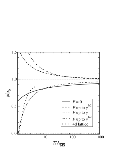
Figure 1: Perturbative pressure vs. lattice data for $N_{f}=0$ (from [6]). The notation is like in Eq. (5), corresponding to $p$ up to $g^{2}$, $g^{3}$, $g^{4}$ and $g^{5}$.

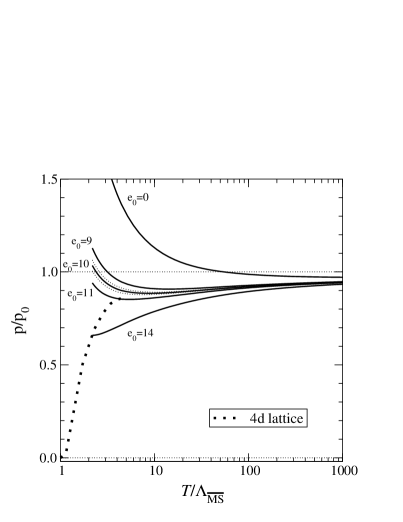
Figure 2: The pressure after inclusion of the long-distance part according to Eq. (6) (from [6]). Statistical errors are shown only for $e_{0}=10$.

As a first result obtained along the strategy outlined above, Fig. 2 shows the normalized pressure. The integration constant has been fixed perturbatively on the 3-loop level, allowing for an additional constant $e_{0}$, which represents an (up to now) unknown $g_{3}^{6}$ contribution. In principle, this constant can be determined in a setup equivalent to the above, after splitting off its perturbative part: A further reduction step relates $e_{0}$ to the free energy of 3d pure gauge theory, which is at the core of the famous non-perturbative $g^{6}$ term, but can nevertheless be determined on the lattice. On the lattice side, we have only included the quadratic scalar condensate, while at temperatures closer to $T_{c}$, the quartic one will become important as well.

While more work is required (and in progress), we wish to point out two important trends seen in Figs. 2,2: First, the outcome is sensitive to the non-perturbative parameter $e_{0}$, which in principle can be determined by additional computations. Clearly, there exists a range for that parameter (say, ${\cal O}(10)$), which leads to a sensible result.

Second, at $T>30{\Lambda_{\overline{\rm MS}}}$ the curves for $g^{5}$ ($y^{{\frac{1}{2}\,}}$) and $e_{0}=10$ fall almost on top of each other, signalling a cancellation of all higher-order terms (determined here by the quadratic Higgs condensate) against the large non-perturbative $g^{6}$ contribution. Hence, in this temperature range the pressure is indeed dominated by short-distance effects.

While we have mostly presented results for QCD at $N_{f}=0$ and zero baryon number, inclusion of $N_{f}$ fermion flavours as well as a baryon chemical potential $\mu_{b}$ pose no further complications, and hence provide for a natural extension of this investigation.

Acknowledgements. This work was supported in part by the EU TMR network ERBFMRX-CT-970122. It is a pleasure to thank K. Kajantie, M. Laine and K. Rummukainen for an enjoyable collaboration on the matter presented in the above.

References

- [1]
- [2] G. Boyd et al, Nucl. Phys. B 469 (1996) 419 [hep-lat/9602007].
- [3] F. Karsch; E. Laermann; Proceedings of Statistical QCD, Bielefeld, 2001.
- [4] C. Zhai and B. Kastening, Phys. Rev. D 52 (1995) 7232 [hep-ph/9507380].
- [5] E. Braaten; J.P. Blaizot; A. Rebhan; A. Peshier; Proceedings of Statistical QCD, Bielefeld, 2001.
- [6] K. Kajantie et al, Phys. Rev. Lett. 86 (2001) 10 [hep-ph/0007109].
- [7] E. Braaten and A. Nieto, Phys. Rev. D 53 (1996) 3421 [hep-ph/9510408].
- [8] K. Kajantie et al, Nucl. Phys. B 503 (1997) 357 [hep-ph/9704416].
- [9] D.J. Gross et al, Rev. Mod. Phys. 53 (1981) 43.
- [10] K. Kajantie et al, hep-ph/0109100.
- [11] J.M. Luttinger and J.C. Ward, Phys. Rev. 118 (1960) 1417.
- [12] P. Cvitanović, Field Theory, Nordita Lecture Notes (Nordita, Copenhagen, 1983).