Identification of Randall-Sundrum Graviton Resonances at Linear Colliders

Abstract

We discuss several methods which can be used to distinguish the graviton resonances of the Randall-Sundrum model from the graviton-like resonances which may occur in other theories. The Breit-Wigner line shape of the RS graviton is found to be particularly useful. In particular we show that the “effective” graviton resonance present in the model of Dvali et al. can be distinguished from those of the Randall-Sundrum scenario for a reasonably wide range of model parameters.

I Introduction and Background

Many models of new physics beyond the Standard Model can lead to phenomena which produce similar signatures at future colliders. It will thus be necessary to have tools available with which to distinguish these models and to identify the specific new physics source. In this report we consider the set of diagnostic tools for model identification of spin-2 resonances and demonstrate that the excitation line shape can be a useful model discriminator.

One class of possible of new physics scenarios is that of extra spatial dimensions at the TeV scale which have been discussed in various contexts for some timeanton . Amongst this class of theories is the interesting and phenomenologically rich model of Randall and Sundrum(RS)rs which predicts the existence of graviton resonances that can be produced at high energy collidersdhr . Such resonances are easily distinguishable from other new states, such as a $Z^{\prime}$snow , by measurements of the angular distribution of their decay products by which one can determine the spin of the initially decaying particle. The question we would like to address below is whether RS gravitons can be distinguished from other spin-2 states which can arise in extra dimensional scenarios. Here we are interested in the particular case where only the lightest of the RS resonances is accessible to detailed accelerator study, i.e., when the other more massive graviton excitations are beyond the collider center of mass energy. (Having a visible series of resonance states would obviously make the situation easier. For example, a determination that the mass spectrum of a series of spin-2 resonances follows the pattern of the roots of the Bessel function $J_{1}$ would strongly favor the RS interpretation.) For some scenarios the model differentiation is quite straightforward, e.g., in the case of Regge-like, spin-2 excitations of the photon and $Z$cpp . Here one finds that the branching fractions for these spin-2 states do not match those for gravitons so that these two models are easily separable given sufficient statistics and the visibility of the relevant final states at a given collider. In other cases, however, the situation may be more difficult, particularly so if the resonance appears more graviton-like. A good example of this is provided by the work of Carena et al.(CDLPQW)cdlpqw that is based on the model by Dvali and co-workersdvali which predicts the existence of a single graviton-like resonance.

II Analysis

In this class of models the propagator of the graviton obtains a rather complicated structure that arises due to novel brane interactions, including a dimensional-dependent, as well as energy-dependent, imaginary part and a real part which vanishes at a fixed value of $s$. Hence one produces an effective resonance which is is some sense a “collective” mode. Since this mode is constructed out of a superposition of the KK states in the graviton tower it has the same branching fractions as does an RS graviton and thus the two models cannot be distinguished using such measurements. The Dvali et al. model has three parameters: $d\geq 2$, the number of extra dimensions, $M_{d}$, the effective resonance mass and $M_{*}$, the $d-$dimensional Planck scale, which is on the order of a few TeV. Note that in the limit $M_{d}\rightarrow\infty$ we recover the model of Arkani-Hamed, Dimopoulos and Dvali(ADD)nima within this framework. For some values of the parameters the effective resonance shape looks very much like that of a relativistic Breit-Wigner(BW) RS graviton; this can easily be seen in Fig. 1. Here is shown the cross section for $e^{+}e^{-}\rightarrow\mu^{+}\mu^{-}$ in both the RS and Dvali et al. models with a common value chosen for the resonance masses(500 GeV) and for various values of the other model parameters. We note that the $d=5$ excitation curve in the Dvali et al. model is quite similar to that for the RS model with the only remaining free parameter $c=k/\overline{M}_{Pl}\simeq 0.1-0.2$. Furthermore, we note that for $d$ and $M$ fixed, increasing $M_{*}$ leads to a narrowing of the width and an increase in the peak height for this effective graviton which also makes the resonance appear more BW-like. This can be seen by examining the curves in Fig. 2. Can the more conventional shape for the RS graviton be distinguished from that of the non-BW “effective” resonance distribution in the Dvali et al. model at a Linear Collider?

     

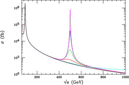
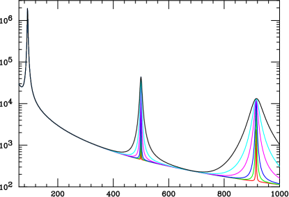
Figure 1: $e^{+}e^{-}\rightarrow\mu^{+}\mu^{-}$ in the Dvali et al.(left) and RS(right) models. For the Dvali et al. case we assume $M_{*}=3$ TeV with $d=2$(red dots) and $d=3,4,5$ and 6(solid red, green, blue and magenta curves). The cyan curve is the ADD model prediction with constructive interference. For the RS model the sample curves are for the parameter $c=k/\overline{M}_{Pl}$ in the range 0.01-0.1.

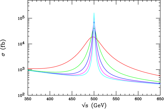
Figure 2: Line shapes for the Dvali et al. graviton-like resonance in $e^{+}e^{-}\rightarrow\mu^{+}\mu^{-}$ assuming $d=5$, $M_{d}=500$ GeV and $M_{*}=3-6$ TeV in steps of 1 TeV corresponding to the red, green, blue, magenta and cyan curves, respectively.

To this end we undertook a preliminary study of the two line shapes which we imagine taking place after an unfolding of the initial state radiation and beamstahlung spectra; in particular we try to fit the non-BW Dvali et al. “effective” resonance under the assumption that it is instead a BW RS graviton and perform a fit for the RS model parameter $c=k/\overline{M}_{Pl}$. A poor quality fit would thus indicate that the two scenarios are distinguishable. In this sample study we imagine the production of a graviton-like resonance(i.e., spin-2 and with the proper branching fractions) with a mass of 1 TeV. We next generate the excitation curves for a set of different resonances in $e^{+}e^{-}\rightarrow\mu^{+}\mu^{-}$ assuming an integrated luminosity of 500 $fb^{-1}$. Since the Dvali et al. resonance shape is non-BW we do not follow the usual approach for fitting a BW but instead we fit a larger $\sqrt{s}$ region surrounding the resonance peak. Given the rather similar shapes of the two resonances we fit the cross section over the region $\sqrt{s}=0.80-1.32$ TeV in steps of 40 GeV. Since this is merely a first pass analysis we make no attempt to optimize the luminosity and assume that the 500 $fb^{-1}$ is shared equally amongst the generated data points; an overall $0.5\%$ luminosity uncertainty is included in this analysis. To test this approach we first try to fit two true RS model resonances with the input values $c=k/\overline{M}_{Pl}=0.073(0.117)$. This comparison is done by employing a series of ‘templates’ which are obtained by generating the relevant cross section data for the RS model for values of $c=k/\overline{M}_{Pl}$ in the range 0.010-0.210 in 200 steps of 0.001. We then perform our fits by using a large order polynomial to interpolate the values of the cross sections at other intermediate values of $c$ for each of the relevant values of $\sqrt{s}$. The fine granularity in the templates insures that the polynomial interpolation gives an extremely accurate estimate for the value of the true cross section. These RS model fits yield $c=0.0730^{+0.0035}_{-0.0040}$ and $c=0.1170^{+0.0026}_{-0.0027}$, respectively, with very good $\chi^{2}$’s as shown in Fig. 3. Next, we attempt to fit the Dvali et al. model; for low values of $M_{*}$ the fits are very poor but improve as $M_{*}$ is increased. Fig. 3 shows the results of these fits when $M_{*}\geq 5$ TeV. For cases where the value of $M_{*}$ are below 5 TeV, the resulting $\chi^{2}$’s are very large and are not shown. Note that the value of both the minimum $\chi^{2}$ and the fitted value for $c$ decrease as $M_{*}$ is increased. Clearly from this figure we see that for values of $M_{*}$ below $\simeq 5.7$ TeV the fit is sufficiently poor to claim that the RS hypothesis fails and the RS and Dvali et al. models are easily distinguished. In particular, for $M_{*}=5.0(5.5)$ TeV we obtain a minimum $\chi^{2}/d.o.f$ of 52.9/13(27.4/13) which corresponds to a confidence level of $1.97\times 10^{-6}(1.70\times 10^{-2})$. However, as we raise $M_{*}$ much beyond $\simeq 5.7$ TeV we obtain an acceptable $\chi^{2}$ and the two models are no longer distinguishable. We would expect to do somewhat better in this separation with an optimised distribution of luminosity; this is currently under investigation.

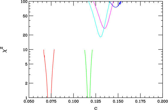
Figure 3: Sample fits to different resonances in $e^{+}e^{-}\rightarrow\mu^{+}\mu^{-}$ assuming the validity of the RS model. The resonance mass is taken to be 1 TeV and a total integrated luminosity of 500$fb^{-1}$ is assumed as described in the text. The red(green) curves are for RS gravitons with $c=k/\overline{M}_{Pl}=0.073(0.117)$ are used as tests of our fitting method. The blue(magenta,cyan) curves are the corresponding fits for the Dvali et al. model with $M_{*}=5.0(5.5,5.7)$ TeV.

III Summary and Conclusions

The above simplified analysis has shown that in some case the line shapes of spin-2 resonances can be a useful tool for model identification of spin-2 resonances at linear colliders. In particular, we have shown in a toy analysis that the line shape can be used to distinguish the graviton resonances of the RS model from the “collective” resonance present in the Dvali et al. model over a reasonable range of model parameters even without an optimization of the luminosity distribution in the resonance region. A detector simulation along the lines of the present analysis including such an optimization would prove useful.

References

- (1) See, for example, I. Antoniadis, Phys. Lett. B246, 377 (1990); I. Antoniadis, C. Munoz and M. Quiros, Nucl. Phys. B397, 515 (1993); I. Antoniadis and K. Benalki, Phys. Lett. B326, 69 (1994)and Int. J. Mod. Phys. A15, 4237 (2000); I. Antoniadis, K. Benalki and M. Quiros, Phys. Lett. B331, 313 (1994).
- (2) L. Randall and R. Sundrum, Phys. Rev. Lett. 83, 3370 (1999).
- (3) For an overview of the Randall-Sundrum model phenomenology, see H. Davoudiasl, J.L. Hewett and T.G. Rizzo, Phys. Rev. Lett. 84, 2080 (2000); Phys. Lett. B493, 135 (2000); and Phys. Rev. D63, 075004 (2001).
- (4) For a review of new gauge boson physics at colliders and details of the various models, see J.L. Hewett and T.G. Rizzo, Phys. Rep. 183, 193 (1989); M. Cvetic and S. Godfrey, in Electroweak Symmetry Breaking and Beyond the Standard Model, ed. T. Barklow et al., (World Scientific, Singapore, 1995), hep-ph/9504216; T.G. Rizzo in New Directions for High Energy Physics: Snowmass 1996, ed. D.G. Cassel, L. Trindle Gennari and R.H. Siemann, (SLAC, 1997), hep-ph/9612440; A. Leike, Phys. Rep. 317, 143 (1999).
- (5) S. Cullen, M. Perelstein and M.E. Peskin, Phys. Rev. D62, 055012 (2000).
- (6) M. Carena, A. Delgado, J. Lykken, S. Pokorski, M. Quiros and C.E.M. Wagner, Nucl. Phys. B609, 499 (2001).
- (7) G. Dvali, G. Gabadadze and M. Porrati, Phys. Lett. B485, 208 (2000); G. Dvali and G. Gabadadze, Phys. Rev. D63, 065007 (2001).
- (8) N. Arkani-Hamed, S. Dimopoulos, and G. Dvali, Phys. Lett. B429, 263 (1998), and Phys. Rev. D59, 086004 (1999); I. Antoniadis, N. Arkani-Hamed, S. Dimopoulos, and G. Dvali, Phys. Lett. B436, 257 (1998).