Inclusive Higgs Production at Next-to-Next-to-Leading Order

Abstract

We describe the contributions of virtual corrections and soft gluon emission to the inclusive Higgs boson production cross section $pp\to H+X$ computed at next-to-next-to-leading order in the heavy top quark limit. We also discuss estimates of the leading non-soft corrections.

I Introduction

The Standard Model is almost thirty-five years old, and its essential goal, to describe the electro-weak interactions as a spontaneously broken $SU(2)_{L}\otimes U(1)_{Y}$ gauge symmetry has been spectacularly confirmed. However, the agent of electroweak symmetry breaking remains elusive. The simplest model of symmetry breaking, called the Minimal Standard Model, uses a single complex doublet of fundamental scalars and is the benchmark for studies of the symmetry breaking sector of the theory. Direct search limits from LEP tell us that the Higgs mass is greater than $\sim 114$ GeV. Fits to precision electroweak data prefer a mass well below the direct search limit although the $95\%$ confidence level upper limit is somewhat greater than $200$ GeV.

Higgs boson production at hadron colliders is dominated by the gluon fusion mechanism. However, experiments must not only produce Higgs bosons, they must also detect them. With a center-of-mass energy of $2$ TeV, the Fermilab Tevatron is primarily sensitive to a Higgs boson with mass below the threshold for decay into $W$ boson pairs. In this case, the Higgs will decay almost exclusively into $b\bar{b}$ pairs which will be undetectable on top of an enormous QCD background. Since the total cross section is too small to permit the use of rare decay modes, a light Higgs can only be detected through associated production with a $W$ or $Z$ boson. Only if the Higgs is sufficiently massive that the $WW^{*}$ channel begins to open up, will inclusive production via the gluon fusion mechanism be useful in the Tevatron Higgs search.

At the CERN LHC, however, gluon fusion will be the discovery channel for the Higgs. The cross section for light Higgs boson production will be sufficiently large that the rare decay $H\to\gamma\gamma$ can be used up to the point that the $WW^{*}$ channel begins to open up. From that point on, the diboson decays provide a very robust signal.

II Methods

The Higgs boson couples to mass, which presents a problem for hadronic production. Gluons are massless and therefore do not couple directly to the Higgs at all, while the quarks that make up the proton have very tiny masses. Therefore, the dominant production mechanism is gluon fusion via virtual top quark loops. In the limit that the top quark is very heavy, we can integrate out the top and formulate an effective Lagrangian coupling the Higgs boson to the light quarks and gluons Vainshtein et al. (1979, 1980); Voloshin (1986). If we take the light quarks to be massless, the effective Lagrangian takes the form

$${\cal L}_{\rm eff}=C_{1}(\alpha_{s})HG^{a\mu\nu}G^{a}_{\mu\nu},$$ (1)

where $G^{a}_{\mu\nu}$ is the gluon field strength tensor. The coefficient function $C_{1}(\alpha_{s})$ has been computed to order $\alpha_{s}^{4}$Chetyrkin et al. (1997).

The use of the effective Lagrangian allows us to replace massive loop diagrams with point-like interactions. Next-to-leading order (NLO) corrections to inclusive Higgs production have been computed using both the effective Lagrangian Dawson (1991); Djouadi et al. (1991) and the full theory Graudenz et al. (1993); Spira et al. (1995). One expects that the effective Lagrangian will work very well if the Higgs mass is much smaller than twice the top mass but that it will be unreliable for larger masses. In fact, it was found that at NLO the effective Lagrangian does indeed agree very well with the full calculation below the top threshold and was even found to agree to within $10\%$ for Higgs masses as large as $1$ TeV.

It was also found that the NLO corrections are very large, of order $70-100\%$. Such large corrections clearly call for the evaluation of still higher-order terms in order to arrive at a solid theoretical understanding of the process. Since the effective Lagrangian seems to be a valid approximation, especially in the phenomenologically interesting region of Higgs boson masses below $200$ GeV, we have embarked on an effort to compute the full next-to-next-to-leading order (NNLO) corrections in the heavy top limit. In this talk, we will present results for soft plus virtual corrections to inclusive Higgs production Harlander (2000); Harlander and Kilgore (2001a); Catani et al. (2001). These terms are not expected to dominate the full result and for this reason we also discuss an approximation of the formally sub-leading but numerically dominant contribution Krämer et al. (1998).

III The Soft Approximation and Beyond

There are three distinct contributions to inclusive Higgs production at NNLO (see Figure 1): Virtual corrections to two loops, single real radiation to one loop and double real radiation at tree level.

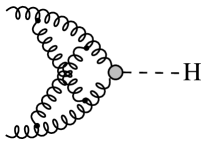
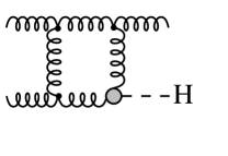
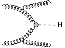
Figure 1: Representative diagrams of virtual corrections, single real radiation and double real radiation.

These three channels produce radiative corrections that fall into three categories, depending on their functional dependence on the fraction $x\equiv M_{H}^{2}/\hat{s}$ of the center-of-mass energy squared of the scattering process that goes into producing the Higgs boson.

$$\sigma^{NNLO}=\ x\left[a\,\delta(1-x)+\sum_{n=0}^{3}b_{n}\left(\frac{\ln^{n}(1-x)}{1-x}\right)_{+}+\sum_{n=0}^{3}c_{n}\ln^{n}(1-x)+\dots\right].$$ (2)

In the virtual corrections, all of the energy goes into Higgs boson production, so these terms contribute only to the $\delta(1-x)$ correction. Real emission processes generate terms like $(1-x)^{n-m\epsilon}$ where $n\geq-1$ is an integer and $\epsilon$ is the dimensional regularization parameter where space-time is taken to be $D=4-2\epsilon$ dimensions. These processes contribute to the $a$ and $b_{n}$ coefficients in equation (2) by expanding terms like $(1-x)^{-1-m\epsilon}$ as distributions

$$(1-x)^{-1-m\epsilon}=\ -\frac{\delta(1-x)}{m\epsilon}+\sum_{n=0}^{\infty}\frac{(-m\epsilon)^{n}}{n!}\left[\frac{\ln^{n}(1-x)}{1-x}\right]_{+}.$$ (3)

In the soft limit, there would be no energy carried away by real emission and only the $\delta(1-x)$ term would be kept. However, the $\left[\frac{\ln^{n}(1-x)}{1-x}\right]_{+}$ terms are directly connected to the $\delta(1-x)$ terms through equation (3) and in canceling the infrared poles proportional to $\delta(1-x)$ we get these terms for free so they are kept as part of the soft approximation.

While the soft approximation keeps the formally leading terms, it was found that at NLO it is a poor approximation. It is actually the sub-leading $c_{n}$ ($n=0,1$ at NLO) terms that dominate the cross section. At NNLO, the $c_{n}$ terms are again expected to dominate. Krämer, Laenen and Spira Krämer et al. (1998) have used collinear resummation to derive approximate NNLO results for $a,b_{n}$ and $c_{n}$. We expect their resummation to give the correct values for the coefficients $b_{3}$, $b_{2}$ and $c_{3}$. The other coefficients require additional calculation, higher order resummation coefficients or, for the remaining $c_{n}$, receive non-collinear contributions and we do not expect the approximation to be accurate. For the $a$ and $b_{n}$ terms which we have computed directly, these expectations are fulfilled, giving us confidence that the dominant term, $c_{3}$ is indeed accurate.

This gives us a range of possibilities for estimating the full NNLO correction. In Figure 2 we show three approximations in addition to the soft limit:
1) Use $c_{3}$, $c_{2}$, $c_{1}$ and $c_{0}$ from Ref. Krämer et al. (1998),
2) Use $c_{3}$ from Ref. Krämer et al. (1998) and generate sub-leading $\ln^{n}(1-x)$ terms by expanding $xb_{n}\to b_{n}+(1-x)b_{n}$,
3) Use $c_{3}$ from Ref. Krämer et al. (1998) and drop all sub-leading $\ln^{n}(1-x)$ terms.
Note that in order to truly estimate the NNLO cross section, one needs NNLO parton distribution functions (PDFs). Unfortunately, the necessary ingredients for producing NNLO PDFs are still being developed. Approximate NNLO PDFs have been produced, but at the time of this work they are not yet publicly available. We therefore use the CTEQ5 NLO parton distribution functions Lai et al. (2000) and acknowledge the inconsistency.

There are two outstanding features of Figure 2: the formally sub-leading $\ln^{3}(1-x)$ terms dominate the corrections, and the size of the corrections is very large. One expects that using NNLO PDFs will reduce the magnitude of the correction by $\sim 10\%$, but it will still be very large. We can take the spread between these approximations as an estimate of the uncertainty due to the uncalculated terms.

IV Conclusions

We have described a calculation of the soft plus virtual NNLO corrections to inclusive Higgs production and estimates of the full NNLO correction based on collinear resummation. While the soft plus virtual terms are perturbatively well-behaved, the leading non-soft terms dominate the cross section and give rise to very large corrections. At this time, the two most important questions concerning inclusive Higgs production are 1) What is the precise value of the NNLO K-factor? and 2) How reliable is the NNLO K-factor with respect to even higher order corrections? The first question can be answered by completing the full NNLO calculation and this work is underway Harlander and Kilgore (2001b). The second question, which is crucial for determining the precision to which the properties of the Higgs boson can be measured at the LHC, requires further investigation.

Figure 2: NNLO K-factor as a function of Higgs boson mass at (a) $\sqrt{\hat{s}}=14$ TeV and (b) $\sqrt{\hat{s}}=2$ TeV. The solid line corresponds to approximation 1 above, the dashed line to approximation 2 and the dash-dot line to approximation 3. The dotted line represents the soft approximation.

References

- Vainshtein et al. (1979) A. I. Vainshtein, M. B. Voloshin, V. I. Zakharov, and M. A. Shifman, Yad. Fiz. 30, 1368 (1979), [Sov. J. Nucl. Phys. 30, 711 (1979)].
- Vainshtein et al. (1980) A. I. Vainshtein, V. I. Zakharov, and M. A. Shifman, Usp. Fiz. Nauk 131, 537 (1980), [Sov. Phys. Usp. 23, 429 (1980)].
- Voloshin (1986) M. B. Voloshin, Yad. Fiz. 44, 738 (1986), [Sov. J. Nucl. Phys. 44, 478 (1986)].
- Chetyrkin et al. (1997) K. G. Chetyrkin, B. A. Kniehl, and M. Steinhauser, Phys. Rev. Lett. 79, 353 (1997), eprint hep-ph/9705240.
- Dawson (1991) S. Dawson, Nucl. Phys. B359, 283 (1991).
- Djouadi et al. (1991) A. Djouadi, M. Spira, and P. M. Zerwas, Phys. Lett. B264, 440 (1991).
- Graudenz et al. (1993) D. Graudenz, M. Spira, and P. M. Zerwas, Phys. Rev. Lett. 70, 1372 (1993).
- Spira et al. (1995) M. Spira, A. Djouadi, D. Graudenz, and P. M. Zerwas, Nucl. Phys. B453, 17 (1995), eprint hep-ph/9504378.
- Harlander (2000) R. V. Harlander, Phys. Lett. B492, 74 (2000), eprint hep-ph/0007289.
- Harlander and Kilgore (2001a) R. V. Harlander and W. B. Kilgore, Phys. Rev. D64, 013015 (2001a), eprint hep-ph/0102241.
- Catani et al. (2001) S. Catani, D. de Florian, and M. Grazzini, JHEP 05, 025 (2001), eprint hep-ph/0102227.
- Krämer et al. (1998) M. Krämer, E. Laenen, and M. Spira, Nucl. Phys. B511, 523 (1998), eprint hep-ph/9611272.
- Lai et al. (2000) H. L. Lai et al. (CTEQ), Eur. Phys. J. C12, 375 (2000), eprint hep-ph/9903282.
- Harlander and Kilgore (2001b) R. V. Harlander and W. B. Kilgore (2001b), in Preparation.