OCTOBER 2001

NEUTRINOS AND THEIR FLAVOR MIXING IN NUCLEAR ASTROPHYSICS

Chapter 1 Introduction

1.1 Motivation

The neutrino was proposed by Pauli in 1929 “….as a desperate remedy to save the principle of energy conservation in beta decay”. This particle which can take part only in weak interactions was discovered experimentally by Reines and Cowan in 1956. Neutrinos can come in different flavors in analogy to the different flavors of charged leptons. However, the decay width of Z⁰ boson in the LEP2 experiment restricts the number of light active neutrinos to three [1]. We now have experimental evidence for the existence of all the three types of neutrinos, ${\nu_{e}}$, ${\nu_{\mu}}$ and ${\nu_{\tau}}$.

The neutrino is known to be a neutral particle which carries a spin 1/2. But whether it has mass or not has been an intriguing issue ever since it was proposed. The direct upper limits on neutrino masses are quite poor. The limit on ${\nu_{e}}$ mass is obtained from tritium beta decay experiments and the best bound is $m_{{\nu_{e}}}<5$ eV [2]. The bounds on ${\nu_{\mu}}$ and ${\nu_{\tau}}$ masses are much more weaker, ${\nu_{\mu}}<$ 190 keV and ${\nu_{\tau}}<$ 18 MeV [3]. If the neutrinos are assumed to be Majorana particles then another experimental bound on neutrino mass comes from the neutrino-less double beta decay experiments ($\beta\beta 0\nu$ or $\beta\beta 0\nu J$, where J is a Majoron). This is a lepton number violating process which will be possible only if the neutrinos are massive Majorana particles. From the non-observation of this process the most stringent bounds on the Majorana neutrino mass is $m_{\nu_{e}}<0.35$ eV at 90% C.L. [4].

Even though these upper bounds, particularly the ones coming from direct mass searches are still weak (these limits on neutrino masses far exceed the cosmological bound which we will discuss later), they clearly indicate that the neutrino masses are much smaller than the mass of the corresponding charged leptons. This leads to an intra-familial hierarchy problem, a challenge for any model which can predict neutrino mass. In the Glashow-Weinberg-Salam standard model of particle physics, which is consistent with all known experimental data till date, the neutrinos are assumed to be massless. However there is no underlying gauge symmetry which forbids neutrino mass, unlike as in the case of the photons. In most extensions of the standard model, the Grand Unified theories and the supersymmetric models, the neutrino is massive [5, 6].

If one does allow for non-zero neutrino mass then the flavor eigenstates of the neutrino can be different from the mass eigenstates. One then encounters the quantum mechanical phenomenon of neutrino flavor mixing where one neutrino flavor oscillates into another flavor due to interference effects. The parameters involved in this process is the mass square difference between the two states which mix, $\Delta{m}^{2}$ and the mixing angle between them, $\theta$. This mechanism can probe very small neutrino masses. Neutrino flavor oscillations was conjectured long ago as a plausible solution to the solar neutrino problem [7] and the atmospheric neutrino anomaly [8].

The thermonuclear fusion reactions responsible for energy generation in the Sun release a huge flux of neutrinos. This flux of pure ${\nu_{e}}$ arriving from the Sun have been measured for almost the last 40 years now by the Homestake, SAGE, GALLEX/GNO, Kamiokande, Super-Kamiokande and the SNO experiments. All these experiments have observed a deficit of the solar neutrino flux predicted by the “standard solar model” (SSM) [9]. This discrepancy between theory and experiment came to be known as the solar neutrino problem. Neutrino flavor mixing – either in vacuum [10] or in solar matter [11] – can account for the solution to this apparent anomaly. The most favored solution to the global data demands a $\mbox{$\Delta{m}^{2}$~{}}\sim 10^{-5}$ eV² and large values for the mixing angle.

The atmospheric neutrinos are produced due to collision of the cosmic ray particles with the air nuclei. These neutrinos were detected in large water $\breve{\rm C}$erenkov experiments which reported a depletion of the ${\nu_{\mu}}$ flux compared to expectation. Solution to this atmospheric neutrino anomaly again called for neutrino flavor oscillations with $\mbox{$\Delta{m}^{2}$~{}}\sim 10^{-3}$ eV² and maximal mixing to reconcile data with predictions. The results from the Super-Kamiokande (SK) atmospheric neutrino experiment in 1998 [8] became a hallmark in the history of particle physics when it finally confirmed that the atmospheric neutrinos do oscillate and are hence indeed massive. The observation of neutrino mass in the SK experiment (although indirect) is the first and till date the only evidence of physics beyond the standard model.

There have been many terrestrial neutrino oscillation searches using both accelerators as well as reactors as neutrino sources [12, 13]. But all of them except the LSND experiment at Los Alamos, have yielded negative results for neutrino oscillations. The LSND experiment has continued to give positive signal for oscillations since 1996 with $\mbox{$\Delta{m}^{2}$~{}}\sim$ eV² [14]. Thus we have three indications of neutrino oscillations. However since the three different hints demand three different values of $\Delta{m}^{2}$ , it is difficult to explain all the experimental data in the framework of three neutrinos. There have been quite a few attempts in the literature to explain all the three experiments with three flavors but it is largely believed that if the LSND results are correct then one has to introduce a fourth sterile neutrino.

Neutrinos are known to play a pivotal role in the supernova dynamics and nucleosynthesis. A huge flux of neutrinos and antineutrinos are released during the thermal cooling phase of a core collapse supernova. These neutrinos can be detected in the terrestrial detectors. The detection of the neutrinos from SN1987A in the Kamiokande and IMB [15] gave birth to the subject of neutrino astronomy and heralded the beginning of a new era in neutrino physics. A careful study of the resultant neutrino signal from a galactic supernova in the terrestrial detectors, can throw light on not just the type-II supernova mechanism but also on the neutrino mass and mixing parameters.

The neutrinos are the most abundant entities in the Universe after radiation. Hence even a small mass for the neutrinos can make a huge difference to the total mass of the Universe. The energy density of the neutrinos cannot exceed the total energy density of the Universe and this puts a strong upper bound on the sum of all the light neutrino species [16], $\sum_{i}m_{\nu_{i}}<46$ eV [5]. Small neutrino masses can be an important component of the dark matter. Since neutrinos were relativistic at the time of structure formation they are called “hot” dark matter. It is believed that a combination of hot+cold dark matter is required for a correct explanation of this problem. Neutrino properties and number of neutrino generations are also severely constrained by primordial nucleosynthesis arguments.

Neutrinos play a crucial role in the understanding of stellar evolution, type-II supernova mechanism, nucleosynthesis and dark matter studies. A huge amount of theoretical and experimental effort has gone into the study of neutrino properties. Thus the importance of the subject warrants a detailed analysis of the neutrino mass and mixing parameters in the context of the current experimental data and a careful study of its implication for astrophysics.

1.2 Plan of Thesis

In this thesis we explore the implications of neutrino oscillations in the context of solar neutrino problem, atmospheric neutrino anomaly and the terrestrial accelerator/reactor neutrino oscillation experiments. We perform detailed statistical analyses of the solar and atmospheric neutrino data and map out the regions of the parameters space consistent with the experiments. We investigate the effect of neutrino mass and mixing on the predicted neutrino signal from a galactic supernova in the current water $\breve{\rm C}$erenkov detectors.

We begin in chapter 2 with the presentation of the basic aspects of neutrino oscillations in vacuum and in matter. We discuss the adiabatic and non-adiabatic propagation of neutrinos in a medium with varying density and present the expressions for the survival probability.

In chapter 3 we give a detailed description of the current status of the neutrino oscillation experiments in terms of two flavor oscillations. For the solar neutrinos we present a brief review of the SSM predictions, summarize the main experimental results, work out the unified formalism for the solar neutrino survival probability, describe our solar neutrino code and perform a comprehensive $\chi^{2}$ analysis of the global solar data. Similarly for the atmospheric neutrinos we discuss the theoretical flux predictions, the SK experimental data, our atmospheric code and perform a $\chi^{2}$ fit with the ${\nu_{\mu}}-{\nu_{\tau}}$ oscillation scenario. We briefly review the bounds from the most important accelerator/reactor experiments.

We extend our study of the solar neutrinos in chapter 4 where we probe the potential of the energy independent solution in describing the global solar neutrino data. We investigate the signatures of this scenario in the future solar neutrino experiments.

In chapter 5 we analyse the SK atmospheric neutrino data and the accelerator/reactor data in a three-generation framework. We present the results of the $\chi^{2}$ analysis of (1) only the SK data and (2) SK+CHOOZ data and compare the allowed regions with those obtained from the accelerator/reactor experiments. For the only SK analysis we indicate some new allowed regions with very small $\Delta{m}^{2}$ which appear due to matter effects peculiar to the mass spectrum of the neutrinos that we have chosen here. We study the implications of this mass spectrum in the K2K experiment.

In chapter 6 we work in a scheme where one of the components in the neutrino beam is unstable and explore the viability of this decay model as a solution to the atmospheric neutrino problem.

In chapter 7 we make quantitative predictions for the number of events recorded in the current water $\breve{\rm C}$erenkov detectors due a galactic supernova. We examine the signatures of neutrino mass and mixing which can show up in the detectors and suggest various variables that can be used to study the effect of oscillations in the resultant signal.

We present our conclusions in chapter 8 with a few comments on the physics potential of the most exciting future detectors.

Chapter 2 Neutrino Oscillations

Neutrino oscillations in vacuum is analogous to $K^{0}-\bar{K^{0}}$ oscillations in its quantum mechanical nature. Neutrinos produced in their flavor eigenstates lack definite mass if they are massive and mixed. The states with definite mass are the mass eigenstates and neutrino propagation from the production to the detection point is governed by the equation of motion of the mass eigenstates. Finally the neutrinos are detected by weak interactions involving the flavor states, leading to the phenomenon of neutrino oscillations, first suggested by Bruno Pontecorvo [1] and later by Maki et al [2]. Some very good reviews on neutrino oscillations include [3, 4, 5, 6, 7, 8].

When neutrinos move through matter they interact with the ambient electrons, protons and neutrons. As a result of this they pick up an effective mass much the same way as photons acquire mass on moving through a medium. This phenomenon has non-trivial impact on the mixing scenario of the neutrinos. In section 2.1 we first develop the formalism for neutrino oscillations in vacuum. In section 2.2 we discuss in detail the effect of matter on the mass and mixing parameters of the neutrinos.

2.1 Neutrino Oscillations in Vacuum

The flavor eigenstate $|\nu_{\alpha}\rangle$ created in a weak interaction process can be expressed as a linear superposition of the mass eigenstates $|\nu_{i}\rangle$

$$|\nu_{\alpha}\rangle=\sum_{i=1}^{N}U_{\alpha i}|\nu_{i}\rangle$$ (2.1)

where $U$ is the unitary mixing matrix analogous to the Cabibo-Kobayashi-Maskawa matrix in the quark sector. We consider the general case of neutrinos with $N$ flavors and henceforth set $\hbar=c=1$. After time t, the initial $|\nu_{\alpha}\rangle$ evolves to

$$|\nu_{\alpha}(t)\rangle=\sum_{i=1}^{N}e^{-iE_{i}t}U_{\alpha i}|\nu_{i}\rangle$$ (2.2)

where $E_{i}$ is the energy of the $i^{th}$ mass eigenstate. For simplicity we assume that the 3-momentum p of the different components of the neutrino beam are the same. The energy $E_{i}$ of the $i^{th}$ component is given by

$$E_{i}=\sqrt{{\bf p}^{2}+m_{i}^{2}}$$ (2.3)

where $m_{i}$ is the mass of the $i^{th}$ mass eigenstate. However since the masses are non-degenerate, the $E_{i}$ are different for the different components and eq. (2.2) is a different superposition of $|\nu_{i}\rangle$ compared to eq. (2.1). Hence one expects the presence of other flavor states in the resultant beam in addition to the original flavor. The amplitude of finding a flavor $\nu_{\beta}$ in the original $\nu_{\alpha}$ beam is

$$\langle\nu_{\beta}|\nu_{\alpha}(t)\rangle=\sum_{i=1}^{N}e^{-iE_{i}t}U_{\alpha i}U_{\beta i}^{*}$$ (2.4)

Hence the corresponding probability is given by

$$P_{\nu_{\alpha}\nu_{\beta}}=\sum_{i=1}^{N}|U_{\beta i}|^{2}|U_{\alpha i}|^{2}+{\rm Re}\sum_{i\neq j}U_{\beta i}^{*}U_{\beta j}U_{\alpha i}U_{\alpha j}^{*}~{}e^{[-i(E_{j}-E_{i})t]}$$ (2.5)

For ultra relativistic neutrinos with a common definite momentum p, $E_{i}\approx{\bf|p|}+\frac{m_{i}^{2}}{2|{\bf p}|}$ and t can be replaced by the distance traveled L. Then we obtain

$$P_{\nu_{\alpha}\nu_{\beta}} = \delta_{\alpha\beta}-4~{}\sum_{j>i}~{}U_{\alpha i}U_{\beta i}^{*}U_{\alpha j}^{*}U_{\beta j}\sin^{2}\left(\frac{\pi L}{\lambda_{ij}}\right)$$ (2.6)

$$\lambda_{ij} = (2.47{\rm m})\left(\frac{E}{MeV}\right)\left(\frac{\rm{eV}^{2}}{\Delta_{ij}}\right)$$ (2.7)

is the oscillation wavelength which denotes the scale over which neutrino oscillation effects can be significant and $\Delta_{ij}=m_{i}^{2}-m_{j}^{2}$. The actual forms of the various survival and transition probabilities depend on the neutrino mass spectrum assumed and the choice of the mixing matrix $U$ relating the flavor eigenstates to the mass eigenstates. The oscillatory character is embedded in the $\sin^{2}\left(\frac{\pi L}{\lambda_{ij}}\right)$ term. Depending on the value of $E$ and $\Delta_{ij}$, if the oscillation wavelength is such that $\lambda_{ij}\gg L$, $\sin^{2}\left(\pi L/\lambda_{ij}\right)\rightarrow 0$, the oscillations do not get a chance to develop and the neutrino survival probability is $\sim 1$. On the other hand, $\lambda_{ij}\ll L$ implies a large number of oscillations, so that once the averaging over energy and/or the distance traveled is done $\sin^{2}\left(\pi L/\lambda_{ij}\right)\rightarrow 1/2$ and one encounters what is called average oscillations. But when $\lambda_{ij}\sim L$ then one has full oscillation effects and constraints on $\Delta_{ij}$ can be put from observations of the resultant neutrino beam.

If we restrict ourselves to two-generations for simplicity then the mixing matrix takes a simple form

$${U\!=\!{\pmatrix{\cos\theta&\sin\theta\cr-\sin\theta&\cos\theta\cr}}}$$ (2.8)

$${\nu_{e}}=\cos\theta\nu_{1}+\sin\theta\nu_{2}$$ (2.9)

$${\nu_{\mu}}=-\sin\theta\nu_{1}+\cos\theta\nu_{2}$$ (2.10)

where $\theta$ is called the mixing angle. The expression of the transition probability from $\nu_{\alpha}$ to a different flavor $\nu_{\beta}$ reduces to

$$P_{\nu_{\alpha}\nu_{\beta}}=\sin^{2}2\theta\sin^{2}\left(\frac{\pi L}{\lambda}\right)$$ (2.11)

The survival probability of the original neutrino beam is simply

$$P_{\nu_{\alpha}\nu_{\alpha}} = 1-P_{\nu_{\alpha}\nu_{\beta}}$$ (2.12)

$$= 1-\sin^{2}2\theta\sin^{2}\left(\frac{\pi L}{\lambda}\right)$$

2.2 Neutrino Oscillations in Matter

So far we have discussed the neutrino transition and survival probabilities in vacuum. When neutrinos move through a medium they interact with the ambient matter and this interaction modifies their effective masses and mixing. It was pointed out in [9, 10] that the patterns of neutrino oscillations might be significantly affected if the neutrinos travel through a material medium. This is because normal matter has only electrons and so the ${\nu_{e}}$ experience both charged as well as neutral current interactions while the ${\nu_{\mu}}$ and ${\nu_{\tau}}$ can participate in only neutral current processes.

Since the flavor eigenstates are involved in weak interactions we work in the flavor basis for the time being and will introduce neutrino mixing later. All the expression for the interaction terms given below are for neutrinos. The corresponding expressions for antineutrinos are same with a -ve sign. The charged current scattering of ${\nu_{e}}$ with electrons gives the following contribution to the Lagrangian

$${\cal L}_{eff}=-\frac{G_{F}}{\sqrt{2}}\{\bar{e}\gamma^{\mu}(1-\gamma_{5}){\nu_{e}}\}\{\bar{\nu_{e}}\gamma_{\mu}(1-\gamma_{5})e\}$$ (2.13)

where $G_{F}$ is the Fermi coupling constant. On rearranging the spinors using Fierz transformation one gets

$${\cal L}_{eff}=-\frac{G_{F}}{\sqrt{2}}\{\bar{\nu_{e}}\gamma^{\mu}(1-\gamma_{5}){\nu_{e}}\}\{\bar{e}\gamma_{\mu}(1-\gamma_{5})e\}$$ (2.14)

For forward scattering of neutrinos off electrons, the neutrino momentum remains the same so that charged current contribution after averaging the electron field over the background becomes

$$-\frac{G_{F}}{\sqrt{2}}\{\bar{\nu_{e}}\gamma^{\mu}(1-\gamma_{5}){\nu_{e}}\}\langle\bar{e}\gamma_{\mu}(1-\gamma_{5})e\rangle$$ (2.15)

The axial current part of $\langle\bar{e}\gamma_{\mu}(1-\gamma_{5})e\rangle$ gives the spin in the non-relativistic limit while the spatial part of the vector component gives the average velocity, both of which are negligible for a non-relativistic collection of electrons. So the only non-vanishing contribution comes from the $\gamma_{0}$ component which gives the electron density.

$$\langle\bar{e}\gamma_{0}e\rangle=n_{e}$$ (2.16)

where $n_{e}$ is the ambient electron density. The extra contribution to the Lagrangian then reduces to $-\sqrt{2}G_{F}n_{e}\bar{\nu}_{eL}\gamma^{0}\nu_{eL}$. Hence for unpolarized electrons at rest, the forward charged current scattering of neutrinos off electron gives rise to an effective potential

$$V_{cc}=\sqrt{2}G_{F}n_{e}$$ (2.17)

The effect of this term is to change the effective energy of the ${\nu_{e}}$ in matter to

$$E_{eff} = \sqrt{{\bf p}^{2}+m^{2}}+\sqrt{2}G_{F}n_{e}$$

$$\approx |{\bf p}|+\frac{m^{2}}{2|{\bf p}|}+\sqrt{2}G_{F}n_{e}$$

$$= |{\bf p}|+\frac{1}{2E}(m^{2}+2\sqrt{2}G_{F}n_{e}E)$$

Thus the charged current interaction gives rise to an extra effective contribution to the ${\nu_{e}}$ mass square called $A$ or the Wolfenstein term [9]

$$A=2\sqrt{2}G_{F}n_{e}E$$ (2.19)

The neutral current contribution to the effective neutrino energies can be calculated in an identical manner and comes out to be

$$V_{nc}=\sqrt{2}G_{F}\sum_{f}n_{f}\left[I_{3L}^{f}-2\sin^{2}\theta_{W}Q^{f}\right]$$ (2.20)

where $f$ stands for the electron, proton or neutron, $n_{f}$ is the density of $f$ in the surrounding matter, $Q^{f}$ is the charge of $f$ and $I_{3L}^{f}$ is the third component of weak isospin of the left chiral projection of $f$. Since for the proton $Q^{f}=1$ and $I_{3L}^{f}=1/2$, while for the electron $Q^{f}=-1$ and $I_{3L}^{f}=-1/2$ and since normal matter is charge neutral ensuring that $n_{e}=n_{p}$, the contributions due to electron and proton cancel each other exactly. Hence the only remaining contribution is due to the neutrons for which $Q^{f}=0$ and $I_{3L}^{f}=-1/2$ so that

$$V_{nc}=-\sqrt{2}G_{F}n_{n}/2$$ (2.21)

In order to see the effect of these extra contributions due to interactions of the neutrino beam with the ambient matter, on neutrino mass and mixing parameters, let us look at the equation of motion for the neutrino states. We restrict ourselves to a two-generation scheme for simplicity (${\nu_{e}}$ mixing with either ${\nu_{\mu}}$ or ${\nu_{\tau}}$) and first write down the evolution equation for the mass eigenstates in vacuum which can be subsequently extended to include matter effects. The equation of motion for the mass eigenstates in vacuum can be written as

$$i\frac{d}{dt}{\pmatrix{\nu_{1}\cr\nu_{2}\cr}}=M^{2}{\pmatrix{\nu_{1}\cr\nu_{2}\cr}}$$ (2.22)

where $M^{2}$ is the mass matrix, diagonal in the mass basis

$$M^{2}\!=\!{\pmatrix{E_{1}&0\cr 0&E_{2}\cr}}\!\approx\!E\!+\!{\pmatrix{m_{1}^{2}/2E&0\cr 0&m_{2}^{2}/2E\cr}}$$ (2.23)

As the interaction terms are defined in the flavor basis we have to look at the evolution equation in the flavor basis. Since the mass eigenstates are related to the flavor eigenstates by the relation (2.1) and since the mixing matrix in two-generations is given by (2.8), the equation of motion in terms of the flavor states can be written as

$$i\frac{d}{dt}{\pmatrix{{\nu_{e}}\cr{\nu_{\mu}}\cr}}=M_{f}^{2}{\pmatrix{{\nu_{e}}\cr{\nu_{\mu}}\cr}}$$ (2.24)

$$M_{f}^{2} = U~{}M~{}U^{\dagger}$$ (2.25)

$$= E+\frac{m_{1}^{2}+m_{2}^{2}}{4E}+\frac{\Delta}{4E}{\pmatrix{-\cos 2\theta&\sin 2\theta\cr\sin 2\theta&\cos 2\theta\cr}}$$ (2.26)

where $M_{f}^{2}$ is the vacuum mass matrix in the flavor basis and $\Delta=m_{2}^{2}-m_{1}^{2}$. We next include in the mass matrix the interaction terms in the mass matrix for neutrinos moving through matter. Once these extra contributions to the Hamiltonian due to interactions of the neutrino with matter are taken into account, the equation of motion for the neutrino beam in the flavor basis is given by eq. (2.24) with the $M_{f}^{2}$ in vacuum replaced with $M_{fm}^{2}$ in matter given by

$$M_{fm}^{2} = E+\frac{m_{1}^{2}+m_{2}^{2}}{4E}-\frac{1}{\sqrt{2}}G_{F}n_{n}$$ (2.27)

$$+\frac{1}{4E}{\pmatrix{4\sqrt{2}G_{F}n_{e}E-\Delta\cos 2\theta&\Delta\sin 2\theta\cr\Delta\sin 2\theta&\Delta\cos 2\theta\cr}}$$

$$= E+\frac{m_{1}^{2}+m_{2}^{2}}{4E}-\frac{1}{\sqrt{2}}G_{F}n_{n}+\frac{A}{4E}$$

$$+\frac{1}{4E}{\pmatrix{A-\Delta\cos 2\theta&\Delta\sin 2\theta\cr\Delta\sin 2\theta&-A+\Delta\cos 2\theta\cr}}$$

where $A=2\sqrt{2}G_{F}n_{e}E$ as defined before. The terms proportional to the identity matrix play absolutely no role in flavor mixing and can be safely dropped. Hence we see that the neutral current term which affect all the flavors equally, falls out of the oscillation analysis and the only non-trivial contribution comes from the charged current interaction.

The energy eigenvalues in matter are obtained by diagonalising the mass matrix $M_{fm}^{2}$. We define $E_{i}^{m}$ to be the mass eigenvalues and $U_{m}$ to be the mixing matrix in matter. In analogy with the vacuum case $U_{m}$ can be parametrized as

$$\pmatrix{{\nu_{e}}\cr{\nu_{\mu}}\cr}=U_{m}\pmatrix{\nu_{1}^{m}\cr\nu_{2}^{m}\cr}$$ (2.28)

$${U_{m}\!=\!{\pmatrix{\cos\theta_{m}&\sin\theta_{m}\cr-\sin\theta_{m}&\cos\theta_{m}\cr}}}$$ (2.29)

where $\theta_{m}$ is the mixing angle in matter. Then since

$$U_{m}^{\dagger}M_{fm}^{2}U_{m}=\!{\pmatrix{E_{1}^{m}&0\cr 0&E_{2}^{m}\cr}}$$ (2.30)

the eigenvalues of the mass matrix are

$$E_{i}^{m}=E-\frac{1}{\sqrt{2}}G_{F}n_{n}+\frac{M_{i}^{2}}{2E}$$ (2.31)

where

$$M_{1,2}^{2}=\frac{1}{2}\left[(m_{1}^{2}+m_{2}^{2}+A)\mp\sqrt{(-A+\Delta\cos 2\theta)^{2}+(\Delta\sin 2\theta)^{2}}\right]$$ (2.32)

Hence the mass squared difference $\Delta$ in vacuum is modified in presence of matter to

$$\Delta_{m}=\left[(-A+\Delta\cos 2\theta)^{2}+(\Delta\sin 2\theta)^{2}\right]^{1/2}$$ (2.33)

while the mixing angle in matter is given by

$$\tan 2\theta_{m}=\frac{\Delta\sin 2\theta}{-A+\Delta\cos 2\theta}$$ (2.34)

or equivalently

$$\sin^{2}2\theta_{m}=\frac{(\Delta\sin 2\theta)^{2}}{(-A+\Delta\cos 2\theta)^{2}+(\Delta\sin 2\theta)^{2}}$$ (2.35)

The mass and the mixing angle in matter are changed substantially compared to their vacuum values depending on the value of $A$ relative to $\Delta$. This change is most dramatic when the condition

$$A=\Delta\cos 2\theta$$ (2.36)

is satisfied. If this condition is attained in matter then $\sin^{2}2\theta_{m}=1$ and the mixing angle in matter become maximal irrespective of the value of the mixing angle in vacuum. So even a small mixing in vacuum can be amplified to maximal mixing due to matter effects This is called the matter enhanced resonance effect or the the Mikhevey-Smirnov-Wolfenstein or the MSW effect [9, 10, 11] which is the favored solution to the Solar Neutrino Problem, a subject we shall address later in great details. Note that for $\Delta>0$ one encounters this resonance for neutrinos ($A>0$) only if $\theta<\pi/4$. Also note that the expression (2.34) can be rewritten as

$$\tan 2\theta_{m}=\frac{\tan 2\theta}{1-n_{e}^{pr}/n_{e}^{res}}$$ (2.37)

where $n_{e}^{pr}$ is the electron density at the point of neutrino production and $n_{e}^{res}$ is the corresponding density at resonance. So that for $n_{e}^{pr}\gg n_{e}^{res}$ the mixing angle in matter $\theta_{m}\rightarrow\pi/2$.

We next look for the electron neutrino survival probability. For a constant density medium the survival probability is given by

$$P_{{\nu_{e}}{\nu_{e}}} = 1-\sin^{2}2\theta_{m}\sin^{2}\left(\frac{\pi L}{\lambda_{m}}\right)$$ (2.38)

$$\lambda_{m} = (2.47{\rm m})\left(\frac{E}{MeV}\right)\left(\frac{\rm{eV}^{2}}{\Delta_{m}}\right)$$ (2.39)

Hence for a constant density medium the expressions for transition and survival probabilities are exactly similar to ones for the vacuum case, with the mass squared difference and the mixing angle replaced by the corresponding terms in matter. But things get more complicated when the neutrinos move through a medium of varying density. We address this complex issue in the next section.

2.2.1 Neutrino Survival Probability in Medium with Varying Density

In most situations encountered in nature the neutrinos propagate through medium with varying density. Since the eigenstates and the eigenvalues of the mass matrix both depend on the density of the medium, the mass eigenstates defined in eq. (2.28) are no longer the stationary eigenstates. For varying density one can define the stationary eigenstates only for the Hamiltonian at a given point. Starting from the equation of motion in the flavor basis and dropping the irrelevant terms proportional to the identity matrix we have

$$i\frac{d}{dx}{\pmatrix{{\nu_{e}}\cr{\nu_{\mu}}\cr}} = \frac{1}{4E}{\pmatrix{A-\Delta\cos 2\theta&\Delta\sin 2\theta\cr\Delta\sin 2\theta&-A+\Delta\cos 2\theta\cr}}{\pmatrix{{\nu_{e}}\cr{\nu_{\mu}}\cr}}$$ (2.40)

$$= \frac{1}{2E}U_{m}{\pmatrix{M_{1}^{2}&0\cr 0&M_{2}^{2}\cr}}{\pmatrix{\nu_{1}^{m}\cr\nu_{2}^{m}\cr}}$$

where we have substituted $x$ for $t$. Keeping in mind that the mixing matrix is now $x$ dependent we obtain

$$i\frac{d}{dx}{\pmatrix{\nu_{1}^{m}\cr\nu_{2}^{m}\cr}} = \left[\frac{1}{2E}{\pmatrix{M_{1}^{2}&0\cr 0&M_{2}^{2}\cr}}-U_{m}^{\dagger}i\frac{d}{dx}U_{m}\right]{\pmatrix{\nu_{1}^{m}\cr\nu_{2}^{m}\cr}}$$ (2.41)

$$= {\pmatrix{M_{1}^{2}/2E&-id\theta_{m}/dx\cr id\theta_{m}/dx&M_{2}^{2}/2E\cr}}{\pmatrix{\nu_{1}^{m}\cr\nu_{2}^{m}\cr}}$$

The off diagonal terms in eq. (2.41) mix the states $\nu_{1}^{m}$ and $\nu_{2}^{m}$ and the mass eigenstates in matter keep changing with $x$. Hence one has to solve the eq. (2.41) to get the survival and transition probabilities. However the mass eigenstates travel approximately unchanged and unmixed as long as the off diagonal terms in (2.41) are small compared to the diagonal terms. Since the terms proportional to the unit matrix do not affect oscillation probabilities, the only physical parameter in the diagonal elements is their difference. Thus the condition for the off diagonal term to be small can be written as

$$\left|\frac{d\theta_{m}}{dx}\right|\ll\left|\frac{M_{2}^{2}-M_{1}^{2}}{4E}\right|$$ (2.42)

This is called the adiabatic condition. Since $|d\theta_{m}/dx|$ has a maximum at resonance while $|M_{2}^{2}-M_{1}^{2}|$ has a minimum, the adiabaticity condition becomes most stringent at the resonance. One can define an adiabaticity parameter as

$$\gamma=\frac{\Delta\sin^{2}2\theta}{2E\cos 2\theta}\left|\frac{d}{dx}lnn_{e}\right|_{x=x_{res}}^{-1}$$ (2.43)

The adiabatic condition then reduces to $\gamma\gg 1$. Depending on whether the adiabatic condition is satisfied or not neutrino propagation in matter may be of two types: adiabatic and non-adiabatic.

$\bullet$The Adiabatic Case: If one can neglect the off diagonal terms in eq. (2.41) in comparison to the diagonal elements, $\nu_{1}^{m}$ and $\nu_{2}^{m}$ approximately become the eigenstate of the mass matrix. This is the adiabatic approximation. As long as the adiabatic condition is satisfied, the two mass states evolve independently and there is no mixing between them. The $\nu_{i}^{m}$ state created in matter then remains a $\nu_{i}^{m}$ always. This is the adiabatic propagation of neutrinos in matter. Adiabatic propagation of neutrinos in matter has very interesting consequences. For example, consider the neutrinos produced at the center of the Sun or a supernova. Since the matter density at the point of production of these neutrinos is much higher that the resonance density, the mixing angle $\theta_{m}\approx\pi/2$ and since

$${\nu_{e}}=\cos\theta_{m}\nu_{1}^{m}+\sin\theta_{m}\nu_{2}^{m}$$ (2.44)

the ${\nu_{e}}$ are created almost entirely in the heavier $\nu_{2}^{m}$ state. Thereafter the neutrino moves adiabatically towards lower densities, crosses the resonance when $A=\Delta\cos 2\theta$ and finally comes out into the vacuum. Since the motion was adiabatic the heavier state remains the heavier state even after it comes out. Since in vacuum the heavier state is

$$\nu_{2}=-\sin\theta{\nu_{e}}+\cos\theta{\nu_{\mu}}$$ (2.45)

the survival probability of the electron neutrino is just $\sin^{2}\theta$. Hence for very small values of the mixing angle $\theta$ one may have almost complete conversion of the ${\nu_{e}}$ produced inside the sun.

In the discussion above the survival probability is $\sin^{2}\theta$ for $\theta_{m}=\pi/2$. For any general angle $\theta_{m}$ at the production point of the neutrino, the survival probability is

$$P_{{\nu_{e}}{\nu_{e}}}=\frac{1}{2}+\frac{1}{2}\cos 2\theta\cos 2\theta_{m}$$ (2.46)

$\bullet$The Non-Adiabatic case: One may encounter cases where $\gamma\sim 1$ and the adiabatic condition (2.42) is not satisfied. This breakdown of adiabaticity is most pronounced at the position of resonance as discussed in the previous section. This violation of adiabaticity at the resonance signals that the off diagonal terms in eq. (2.41) become comparable to the diagonal terms and there is a finite probability of transition from one mass eigenstate to another. This transition probability between the mass eigenstates is called the level crossing or the jump probability. It is defined as

$$P_{J}=\left|\langle\nu_{2}^{m}(x_{+})|\nu_{1}^{m}(x_{-})\rangle\right|^{2}$$ (2.47)

where $x_{\pm}$ refer to two faraway points on either side of the resonance. $P_{J}$ can be determined by solving the equation of motion (2.41) for a given matter density profile. For a linearly varying density, the jump probability is given by the Landau-Zener expression [12, 13]

$$P_{J}=\exp(-\frac{\pi}{2}\gamma)$$ (2.48)

where $\gamma$ is the adiabaticity parameter given by eq. (2.43). For the Sun the density profile is roughly exponential and we will address that issue in the next chapter.

The electron neutrino survival probability, taking into account the finite level crossing between the mass eigenstates due to breakdown of adiabaticity is given by

$$P_{{\nu_{e}}{\nu_{e}}}=\frac{1}{2}+(\frac{1}{2}-P_{J})\cos 2\theta\cos 2\theta_{m}$$ (2.49)

This can be easily computed if one knows the form of $P_{J}$.

2.2.2 Matter Effects with Sterile Neutrinos

In the entire discussion above on the effect of matter on neutrino mass and mixing we had tacitly assumed that both the flavors involved in oscillations were active flavors, that is, can take part in weak interactions. But one may consider situations where one of the states involved is sterile. Sterile states have no interactions with the surrounding medium, neither charged nor neutral. Thus for the ${\nu_{e}}-\nu_{\rm sterile}$ mixing, relevant for the solar neutrino problem, the mixing angle and the mass squared difference in matter are given by,

$$\Delta_{m} = \left[(-2\sqrt{2}G_{F}n_{e}E+\sqrt{2}G_{F}n_{n}E+\Delta\cos 2\theta)^{2}+(\Delta\sin 2\theta)^{2}\right]^{1/2}$$ (2.50)

$$\tan 2\theta_{m} = \frac{\Delta\sin 2\theta}{-2\sqrt{2}G_{F}n_{e}E+\sqrt{2}G_{F}n_{n}E+\Delta\cos 2\theta}$$ (2.51)

The survival probability $P_{{\nu_{e}}{\nu_{e}}}$ is still given by eqs. (2.46) and (2.49). For the ${\nu_{\mu}}-\nu_{\rm sterile}$ mixing, relevant for the atmospheric neutrino anomaly the corresponding expressions are

$$\Delta_{m} = \left[(\sqrt{2}G_{F}n_{n}E+\Delta\cos 2\theta)^{2}+(\Delta\sin 2\theta)^{2}\right]^{1/2}$$ (2.52)

$$\tan 2\theta_{m} = \frac{\Delta\sin 2\theta}{\sqrt{2}G_{F}n_{n}E+\Delta\cos 2\theta}$$ (2.53)

Note however that whether the neutrinos are oscillating into active or sterile species matter only when a material medium is involved. The oscillations in vacuum is the same for both the cases.

Chapter 3 Bounds on Two Flavor Neutrino Mixing Parameters

The question whether neutrinos are massive or not has been answered. The Super-Kamiokande (SK) atmospheric neutrino data has quelled all apprehensions about the existence of neutrino flavor mixing and has propelled neutrino physics to the forefront of particle phenomenology. The other puzzle which has warranted neutrino oscillations as a plausible solution is the long standing solar neutrino problem. For the last four decades solar neutrino detectors have recorded a flux far less than that predicted by solar models. Though the theory of neutrino flavor oscillations can offer the best possible solution to this anomaly, there are still a lot of issues that have to be settled. Finally there have been earnest searches for neutrino flavor mixing in the laboratory, using both reactors as well as accelerators as sources for neutrino beams. But all such quests have lead to negative results, with the exception of the LSND experiment at Los Alamos which has reiterated since 1996 to have observed positive neutrino oscillation signals.

In this chapter we survey the current status of the solar neutrino problem, the atmospheric neutrino anomaly and the laboratory experiments. We briefly discuss the incident neutrino fluxes, the detection techniques, present the main experimental results and perform detailed statistical analysis of the solar and the atmospheric neutrino data in terms of two-generation neutrino oscillations. We describe our solar and atmospheric neutrino code and discuss the method of $\chi^{2}$ analysis. We identify the best-fit solutions and display the allowed regions in the neutrino parameter space. We begin with the solar neutrino problem in section 3.1, next take up the case of the atmospheric neutrino anomaly in section 3.2 and finally move over to the description of the most stringent accelerator/reactor experiments in section 3.3.

3.1 The Solar Neutrino Problem

Neutrinos are an essential byproduct of the thermonuclear energy generation process inside the Sun whereby four proton nuclei are fused into an alpha particle.

$$4p~{}\longrightarrow~{}^{4}He+2e^{+}+2{\nu_{e}}+28~{}{\rm MeV}$$ (3.1)

This process is called Hydrogen Burning and is responsible for the hydrostatic equilibrium of the Sun. About 2-3% of the total energy released in the process (3.1) is carried away by the neutrinos. The rest is in the form of electromagnetic radiation, which diffuses out from the core to the surface of the Sun, getting degraded in frequency to appear as sunlight. It takes millions of years for the photons to emerge from the Sun due to interactions with the solar matter. As a result of these repeated scatterings, the photons cannot give us any direct information about the core of the Sun. The neutrinos on the other hand have typical scattering cross sections of about $10^{-43}$ cm², which for a solar density of about 100 g/cc gives a mean free path of the order of $10^{17}$ cm. This is much larger than the radius of the Sun. The neutrinos escape from the Sun unadulterated and bring along, all the information about the solar core imprinted on them. Thus a careful study of these neutrinos promises to provide detailed information about the solar interiors and the thermonuclear energy generation process inside the core and hence holds the potential to verify or refute the existing solar models.

Keeping this in mind, Ray Davis began his pioneering experiment in which neutrinos are captured by the ${}^{37}Cl$ atoms [1]. The corresponding work on theoretical predictions for the solar neutrino fluxes were done by Bahcall and his collaborators [2] in the framework of what is called the “standard solar model”. The first results of this experiment were declared in 1968 [1]. This experiment has been running for almost four decades now [3] and the results have been remarkably robust; the experiment sees a depletion of the solar neutrino flux over the standard solar model (SSM) predictions. The solar neutrinos seem to vanish on their way from the Sun to the Earth and this mystery of missing solar neutrinos constitutes the Solar Neutrino Problem (SNP). Two decades later the Kamiokande water $\breve{\rm C}$erenkov experiment corroborated this observed deficit of solar neutrinos [4]. This conflict between the SSM prediction and observation has been further substantiated by the results from the ${}^{71}Ga$ experiments – the SAGE [5], the GALLEX [6] and now the GNO [7], which is the upgraded version of the GALLEX. The advent of the Super-Kamiokande [8, 9, 10], the upgraded version the the original Kamiokande experiment, brought with it rich statistics, which provided further insight into the SNP in terms of the overall depletion of the solar flux [8], the energy dependence of the suppression rate [9] and the presence of any difference in the observed rate at day and at night, a phenomenon called the day-night effect [10]. The recently declared results on the electron scattering events (ES) from the Sudbury Neutrino Observatory (SNO) [11] are consistent with the observations of SK while their charged current (CC) events when compared with the SK events signify the presence of a ${\nu_{\mu}}/{\nu_{\tau}}$ component in the resultant neutrino beam at the $3.3\sigma$ level while the total solar flux is calculated to be $5.44\pm 0.99\times 10^{6}cm^{-2}s^{-1}$ which is in agreement with the SSM predictions [11].

Thus if the neutrinos are assumed to be the standard particle predicted by the Glashow-Weinberg-Salam standard model of particle physics then there seems to be an apparent discrepancy between the experimental observations and the SSM predictions. There have been several attempts in the literature to explain the experimental results by modifying the solar models, assuming neutrinos to be standard. These endevours are collectively called the astrophysical solutions. In the most general class of these solutions the solar neutrino fluxes are considered as free parameters, with the only requirement being the reproduction of the observed solar luminosity [12]. But all such analyses fail to explain the observations from all the three experiments, Cl, Ga and water $\breve{\rm C}$erenkov simultaneously. In fact the best-fit for these solutions predict a negative flux for the ${}^{7}{Be}$ neutrino which is an unphysical situation. The astrophysical solutions fail to explain even two of the solar neutrino results simultaneously. After the declaration of the SNO results the astrophysical solution has fallen into further disfavor [13, 14]. In [13] Bahcall has shown that while prior to SNO the astrophysical solution failed to fit the data at the $2.5\sigma$ level, after including the SNO data it is ruled out at $4\sigma$. Thus it is not the uncertainties in the solar models that are responsible for this anomaly. In fact the solar models have been remarkably refined in the last four decades and the flux uncertainties have been reduced to a large extent. Hence one needs to consider some non-standard property for the neutrino in order to be able to reconcile the data with the standard solar model predictions.

Among the various particle physics solutions proposed till date, neutrino oscillations in vacuum [15] and/or in matter [16, 17], have been the first and the most appealing solution [18, 19, 20, 21, 22]. Neutrino flavor mixing has the potential to explain not only the total suppression of the solar flux, but also the energy dependence of the suppression factor and the day-night asymmetry. The analysis of the solar neutrino problem in terms of neutrino mass and mixing gives four pockets of allowed area in the neutrino oscillation parameter space. One of them has $\mbox{$\Delta{m}^{2}$~{}}\sim 10^{-6}$ eV² and mixing angles very small and is called the small mixing angle (SMA) region. Another has $\mbox{$\Delta{m}^{2}$~{}}\sim 10^{-5}$ eV² with large mixing angles and is referred to as the large mixing angle (LMA) solution. A third allowed zone has $\Delta{m}^{2}$ in the range $10^{-7}-10^{-9}$ eV² and mixing angle close to maximal. This is the LOW-QVO region, LOW stands for low $\Delta{m}^{2}$ and QVO for quasi vacuum oscillations. The last region is the one associated with vacuum neutrino oscillations with $\mbox{$\Delta{m}^{2}$~{}}\sim 10^{-10}$ eV² and mixing close to maximal. While doing an analysis of the solar data one has to consider ${\nu_{e}}$ oscillations to either an active flavor (${\nu_{\mu}}$, ${\nu_{\tau}}$) or some sterile species ($\nu_{\rm sterile}$). The latter case will be different, firstly because the sterile neutrinos will not show up in the detectors in the neutral current interactions even though ${\nu_{\mu}}$, ${\nu_{\tau}}$ can. This feature affects both the MSW as well as the vacuum solutions. For the MSW solutions there is an extra difference as the sterile neutrinos do not have any interaction with the ambient matter, both in the Sun and in the Earth. Thus the effect of matter on the mixing parameters will be different for the $\nu_{\rm sterile}$ as compared to $\nu_{\rm active}$, as discussed in the previous chapter.

We perform detailed $\chi^{2}$ -fits for both the ${\nu_{e}}-\nu_{\rm active}$ and ${\nu_{e}}-\nu_{\rm sterile}$ transformations. We perform a global $\chi^{2}$ analysis of the solar neutrino data from all experiments in the framework of neutrino mass and mixing. We adopt an unified approach for the presentation of the MSW, the vacuum and quasi-vacuum oscillations solutions. We find the best-fit solution to the global data and show the allowed regions in the $\Delta{m}^{2}$ -$\tan^{2}\theta$ parameter space. From the global analysis of all available solar neutrino data, one finds that the large mixing angle ${\nu_{e}}-\nu_{\rm active}$ MSW solution gives the best fit.

Section 3.1.1 is a brief discussion on the solar neutrino flux predictions in the standard solar models and the various uncertainties involved. In section 3.1.2 we briefly present the essential features of the solar neutrino experiments and summarize their main results. In section 3.1.3 we discuss the solar neutrino code developed by us. In section 3.1.4 we introduce neutrino flavor mixing and develop the unified formalism for the analysis of the SNP in the context of neutrino mixing. Finally in section 3.1.5 we present the results of a comprehensive $\chi^{2}$ analysis of the solar neutrino data. We identify the best fit solutions and give C.L. allowed areas in the neutrino parameter space.

3.1.1 Neutrinos in Standard Solar Models

“Standard Solar Model” is a solar model constructed with the best available physics and input data. Almost all solar models postulate the thermonuclear fusion of protons (3.1) to be the main energy generation process in the Sun [23, 24, 25, 26, 27, 28, 29]. The eq. (3.1) is actually the compactified form for a chain of reactions in which four hydrogen nuclei are fused to form a helium nucleus. This chain of reactions, called the pp chain is shown in fig. 3.1.

Figure 3.1: The reactions of the $pp$-chain. The probability of a particular reaction is shown as a percentage. The neutrinos are shown underlined. Those with double underlines are monoenergetic. We indicate in parenthesis the popular names by which these various neutrinos are addressed.

The other series of nuclear reactions in the core of the Sun that release neutrinos is the $CNO$ cycle. However, since the $CNO$ cycle becomes important only above core temperature $T_{c}\sim 10^{7}$ K, it produces only about 1.5% of the total solar neutrinos released. Nevertheless the $CNO$ cycle is responsible for three sources of solar neutrinos and we call them the ${}^{13}N$, ${}^{15}O$ and ${}^{17}F$ neutrinos. So one has eight different types of solar neutrinos, five produced in the $pp$ chain and three in the $CNO$ cycle.

From the observed solar luminosity and from the fact that 28 MeV energy are released per two electron neutrinos produced in eq. (3.1), one can make an order of magnitude estimate of the solar neutrino flux

$$\Phi_{\nu_{e}} = \frac{\rm luminosity}{4\pi D^{2}\times\frac{1}{2}(\rm binding~{}energy~{}of~{}^{4}He)}$$ (3.2)

$$\approx \frac{4\times 10^{33}{\rm ergs/s}}{4\pi\times(1.5\times 10^{13}{\rm cm})^{2}\times 14~{}{\rm MeV}}$$

$$\approx 6\times 10^{10}{\rm cm}^{-2}{\rm s}^{-1}$$

The exact solar neutrino flux calculations depend on a number of factors such as the nuclear reactions rates, the metallicity ($Z/X$), the age of the Sun and the opacity. Detailed solar neutrino flux calculations from the standard solar models are available [23, 24, 25, 26, 27, 28, 29] and agree with the rough estimate made in eq. (3.2) in order of magnitude. The first two columns of Table 3.1 list the total solar neutrino fluxes along with their $\pm 1\sigma$ uncertainties, from the eight different reactions, as given by the year 2000 model of Bahcall, Pinsonneault and Basu, which we shall henceforth refer to as BPB00 [29]. In fig. 3.2 we show the energy spectrum of the neutrinos emitted in various reactions of the $pp$ chain in BPB00. Also shown are the $\pm 1\sigma$ uncertainties in the various fluxes.

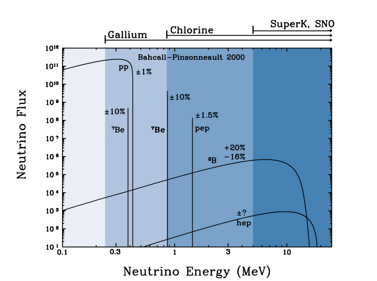
Figure 3.2: Solar neutrino spectrum in the standard solar model as a function of neutrino energy. The continuous spectra are in units of cm^-2MeV^-1s^-1, while the monoenergetic lines are in cm^-2s^-1. Figure shows the $\pm 1\sigma$ uncertainties in the model predictions of the various fluxes. Also shown are the energy ranges over which the solar neutrino experiments are sensitive.

source	Flux	Cl	Ga
	($10^{10}$ cm-2s-1)	(SNU)	(SNU)
$pp$	5.95($1.00^{+0.01}_{-0.01}$)	0.0	69.7
$pep$	1.40$\times 10^{-2}$($1.00^{+0.015}_{-0.015}$)	0.22	2.8
$hep$	9.3$\times 10^{-7}$	0.04	0.1
${}^{7}Be$	4.77$\times 10^{-1}$($1.00^{+0.10}_{-0.10}$)	1.15	34.2
${}^{8}B$	5.05$\times 10^{-4}$($1.00^{+0.20}_{-0.16}$)	5.76	12.1
${}^{13}N$	5.48$\times 10^{-2}$($1.00^{+0.21}_{-0.17}$)	0.09	3.4
${}^{15}O$	4.80$\times 10^{-2}$($1.00^{+0.25}_{-0.19}$)	0.33	5.5
${}^{17}F$	5.63$\times 10^{-4}$($1.00^{+0.25}_{-0.25}$)	0.0	0.1
Total		$7.6_{-1.1}^{+1.3}$	$128_{-7}^{+9}$

Table 3.1: The BPB00 predictions for the solar neutrinos fluxes and neutrino capture rates in the Cl and Ga detectors. The expected ${}^{8}{B}~{}$flux in SK is 5.05$\times 10^{-6}{\rm cm}^{-2}{\rm s}^{-1}$.

Among the predictions for the neutrinos from different reactions in the Sun, the flux of the ${}^{8}B$ neutrino is the most uncertain. In fact the largest contribution to the differences in the predictions of the various standard solar models is their choice of different values for the $S_{17}$ which is the astrophysical $S$-factor for the reaction $(^{7}Be(p,\nu)^{8}B)$. While the SSM of Dar and Shaviv [27] uses a value of $S_{17}$ as low as $17\pm 2$ eV barn, the earlier 1992 and 1995 models of Bahcall and Pinsonneault [24, 26] had used $S_{17}=24\pm 2$ eV barn. The value of $S_{17}$ used in BPB00 is $19^{+4}_{-2}$ eV barn which is the value accepted by the Institute of Nuclear Theory (INT) [30].

The solar fluxes are sensitive not just to the uncertainties in the nuclear reaction rates, but also to the value of the core temperature $T_{c}$. In fact the ${}^{8}{B}~{}$flux $\Phi_{{}^{8}B}\propto T_{c}^{18}$, the $pp$ flux $\Phi_{pp}\propto T_{c}^{-1.5}$ while the ${}^{7}{Be}$ flux $\Phi_{{}^{7}Be}\propto T_{c}^{8}$. Hence even a slight increase in the value of $T_{c}$ can seriously affect all the solar fluxes. In particular, it will sharply raise the ${}^{8}{B}~{}$and ${}^{7}{Be}$ fluxes and lower the $pp$ flux. The value of $T_{c}$ is sensitive to a number of factors including the value of the opacity of the solar core. If the value of the opacity is raised, it slows down the heat transport, leading to higher core temperatures. The value of the opacity in turn depends on the abundance of heavy elements in the Sun or the metallicity. Another very important ingredient in the solar models is the inclusion of element diffusion. Apart from convection, the two other mechanisms important for transporting solar matter are; (1) gravitational settling, which pulls heavier elements towards the center and (2) temperature gradient diffusion, which results in pushing lighter elements outward. Both of these cause the inward diffusion of ${}^{4}He$ and outward diffusion of ${}^{1}H$. Hence diffusion increases the opacity, which results in a higher $T_{c}$ leading to an increase of ${}^{8}B$ and ${}^{7}Be$ fluxes and decrease of the $pp$ flux.

In spite of the various uncertainties involved, only a fraction of which have been discussed above, it was shown in [24, 26] that if the same input physics is used, then all the standard solar models agree with one another to an accuracy of better than 10%. Hence though we have presented the results on the total fluxes and the neutrino spectra from the standard solar model of Bahcall, Pinsonneault and Basu, predictions by almost all the standard models published so far are in reasonable agreement with each other. For our analysis of the SNP in terms of neutrino mass and mixing, we have used the latest SSM predictions by Bahcall, Pinsonneault and Basu (BPB00) [29].

3.1.2 The Solar Neutrino Experiments

The Cl Experiment (Homestake)

This is the first and the longest running experiment on solar neutrinos started in the sixties by Davis and his collaborators with 615 tons of $C_{2}Cl_{4}$ (perchloroethylene) in the Homestake Gold mine in South Dakota [1]. The neutrino detection process in this experiment is

$${\nu_{e}}+\mbox{${}^{37}{Cl}$~{}}\rightarrow^{37}Ar+e^{-}$$ (3.3)

The ${}^{37}Ar$ atoms are extracted from the detectors at the end of a certain period of time and counted by detecting the Auger electron released when the ${}^{37}Ar$ decays by capturing a K-shell or an L-shell electron. The reaction (3.3) has a threshold of 0.814 MeV so that the Cl experiment predominantly detects the ${}^{7}{Be}$ and ${}^{8}{B}~{}$neutrinos. It misses out on the most abundant and least uncertain $pp$ neutrinos which have a maximum energy of only 0.42 MeV (cf. fig 3.2). The third column of Table 3.1 shows the BPB00 predictions [29] for the neutrino capture rates in the Cl experiment for the different neutrino sources. Also shown for the Cl detector are the total predicted rate and the $\pm 1\sigma$ uncertainties in the model calculations. The numbers quoted are in a convenient unit called SNU, defined as, $1~{}{\rm SNU}=10^{-36}{\rm events/target~{}atom/second}$. The observed rate of solar neutrinos in the experiment is [3]

$${\rm Observed~{}Rate}_{\rm Cl}=2.56\pm 0.23~{}{\rm SNU}$$ (3.4)

Compared to the BPB00 prediction of $7.6_{-1.1}^{+1.3}$ as in Table 3.1, this gives a ratio of observed to expected SSM rate of $0.335\pm 0.029$.

The Ga Experiments (SAGE, GALLEX, GNO)

These are also radiochemical experiments that use ${}^{71}{Ga}$ as their detector material. The ${}^{71}{Ga}$ captures a ${\nu_{e}}$ to produce ${}^{71}Ge$ by the reaction

$${\nu_{e}}+\mbox{${}^{71}{Ga}$~{}}\rightarrow^{71}Ge+e^{-}$$ (3.5)

This reaction has a threshold of only 0.233 MeV. Hence the advantage that this detector has is that it is capable of seeing the $pp$ neutrinos which are responsible for 98.5% of the energy generation of the Sun. Hence the fact that the Ga detector could detect these neutrinos confirms the basic postulate of all the solar models, that the Sun generates its energy through thermonuclear burning. This itself was a very significant achievement of the Ga detectors.

The SAGE (Soviet American Gallium Experiment) in Russia and GALLEX (Gallium Experiment) in Italy are experiments that use this detection technique. The SAGE in Baksan Neutrino Observatory uses 60 tons of metallic $Ga$ as the target. The ${}^{71}{Ge}$ produced is separated and counted. The observed rate is [5]

$${\rm Observed~{}Rate}_{SAGE}=75.4\pm^{7.0}_{3.0}(stat.)\pm^{3.5}_{3.0}(syst.)~{}{\rm SNU}$$ (3.6)

The GALLEX is located in the Gran Sasso laboratory in Italy and uses 30 tons of $Ga$ in the form $GaCl_{3}-HCl$ solution. The observed neutrino rate in GALLEX is [6]

$${\rm Observed~{}Rate}_{GALLEX}=77.5\pm^{7.6}_{7.8}~{}{\rm SNU}$$ (3.7)

The GALLEX has now finished its run and has been upgraded to the GNO (Gallium Neutrino Observatory) which has already given results [7]

$${\rm Observed~{}Rate}_{GNO}=65.8\pm^{10.7}_{10.2}~{}{\rm SNU}$$ (3.8)

The combined SAGE and GALLEX+GNO results is

$${\rm Observed~{}Rate}_{Ga}=74.7\pm 5.0~{}{\rm SNU}$$ (3.9)

which is more than 6$\sigma$ away from the SSM predicted rate of $128_{-7}^{+9}$ SNU [29] (cf. Table 3.1).

The Water $\breve{\rm C}$erenkov Experiments (Kamiokande and Super-Kamiokande)

The water $\breve{\rm C}$erenkov detectors detect solar neutrinos by the forward scattering of electrons

$${\nu_{e}}+e^{-}\rightarrow{\nu_{e}}+e^{-}$$ (3.10)

As it moves, the scattered electron emits $\breve{\rm C}$erenkov light, which is viewed by the huge number of photomultiplier tubes covering the entire detector volume. The water detector in general has a higher threshold so that it is sensitive to just the ${}^{8}{B}~{}$and the vanishingly small $hep$ neutrinos. But it has many other advantages. It is a real time experiment which has directional information. The reaction (3.10) is forward peaked and the detector can reconstruct the direction of the incoming neutrino from the angle of the emitted $\breve{\rm C}$erenkov cone. Earlier the Kamiokande [4] and now the Super-Kamiokande [8] have found an excess of events peaking broadly in the solar direction and have thus confirmed that the observed neutrinos are indeed coming from the Sun. The water detector can observe not just the ${\nu_{e}}$ as in the radiochemical experiments, but neutrinos and antineutrinos of all flavors. Thus it can detect ${\nu_{\mu}}$ and ${\nu_{\tau}}$ through neutral current electron scattering though the neutral current scattering cross-section is about $1/6^{th}$ of the charged current scattering cross-section. This is important if one wants to distinguish between neutrinos oscillating out into either ${\nu_{\mu}}/{\nu_{\tau}}$ or to some $sterile$ species $\nu_{\rm sterile}$, which does not have any standard model interactions. But the real strength of this experiment lies in its ability to provide information about the incident neutrino energy spectrum from the observed recoil electron energy spectrum. This piece of experimental observation tells us about the form of the energy dependence of the suppression rate which is extremely important in distinguishing between allowed solutions to the SNP. Also, since it is a real time experiment, it can divide its data set into day and night bins. Hence the detector can give information on the difference between the observed solar flux during day and night.

The Kamiokande experiment, located in a deep mine at Mozumi, Japan, was a 4.5 ktons detector with a threshold of 7.5 MeV. The observed solar neutrino flux reported by this experiment is

$${\rm Observed~{}Rate}_{\rm Kamiokande}=(2.89\pm 0.42)\times 10^{6}{\rm cm}^{-2}{\rm s}^{-1}$$ (3.11)

Super-Kamiokande (SK) [8] is the upgraded version of Kamiokande. The first result of this experiment on solar neutrinos was released in 1998 [8]. The SK has now managed to reduce its threshold to 5.0 MeV [31] and the observed solar flux reported by SK after 1258 day of data taking is [31]

$${\rm Observed~{}Rate}_{\rm SK}=(2.32\pm 0.08)\times 10^{6}{\rm cm}^{-2}{\rm s}^{-1}$$ (3.12)

The recoil electron energy spectrum [9] released by the SK collaboration after 1258 day of data [31] is consistent with no spectral distortion. This means that the suppression rate observed is essentially energy independent. The SK gives not just the total recoil energy spectrum but also the spectrum at day and the spectrum at night. In fig 3.3 we show the day and the night spectra separately for the 1258 day SK data. We can see that both the day and the night spectra are flat upto $1\sigma$. The night bins have slightly more events than the day bins. The degree of difference between the day and night event rates is conveniently measured by the day-night asymmetry, defined as ${\cal A}=(\Phi_{n}-\Phi_{d})/\Phi_{average}$ and $\Phi_{average}=\frac{1}{2}(\Phi_{n}+\Phi_{d})$, where $\Phi_{n}(\Phi_{d})$ is the observed flux during night(day). The SK reports [31]

$${\cal A}=0.033\pm 0.022({\rm stat.})_{-0.012}^{+0.013}({\rm sys.})$$ (3.13)

This is just a $1.3\sigma$ effect which signifies almost no day-night asymmetry.

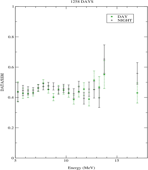
Figure 3.3: SK recoil energy spectra along with the $\pm 1\sigma$ errorbars for 1258 day data. The dotted errorbars are for the spectra at day while the solid errorbars are for the night bins.

In order to study the day-night effect in greater details, the SK divide their data on total rates into a day and five night bins according to the zenith angle at which the neutrinos arrive [10, 31]. They have now also divided their observed spectrum into zenith angle bins [31]. This helps to study the energy dependence of the suppression rate as well as the predicted day night asymmetry together in the most efficient manner.

The Sun-Earth distance changes with the time of the year due to the eccentricity of the Earth’s orbit. If the neutrinos oscillate in vacuum on their way from the Sun to Earth, then one should expect an extra modulation of the solar neutrino flux due to oscillations with the time of the year, as the survival probability depends very crucially on the distance that the neutrinos travel. The SK have reported the seasonal variation of the solar flux. The data is consistent with the expected annual variation due to orbital eccentricity of the Earth assuming no neutrino oscillations.

The Heavy Water Detector (SNO)

The Sudbury Neutrino Observatory at Sudbury, Canada is the worlds first heavy water detector containing 1 kton of pure ${\rm D_{2}O}$ surrounded by 7 kton of pure ${\rm H_{2}O}$. The main detection process is the charged current (CC) breakup of the deuteron

$$\nu_{e}+d\rightarrow p+p+e^{-}$$ (3.14)

It has now declared its first results on the observed ${}^{8}{B}~{}$flux [11]

$$\Phi_{CC}^{SNO}=1.75\pm 0.07(stat)^{+0.12}_{-0.11}(sys)\times 10^{6}{\rm cm}^{-2}{\rm s}^{-1}$$ (3.15)

The detector threshold for the kinetic energy of the observed electron released in (3.14) is 6.75 MeV. SNO has also released its observed ${}^{8}{B}$ flux measured by the electron scattering (ES) reaction (cf. eq. (3.10)) and they report [11]

$$\Phi_{ES}^{SNO}=2.39\pm 0.34(stat)^{+0.16}_{-0.14}(sys)\times 10^{6}{\rm cm}^{-2}{\rm s}^{-1}$$ (3.16)

which agrees with the SK observation (3.12), though the errors are still large. Apart from the total rates, SNO also gives the recoil electron energy spectrum for the CC events and they do not report any significant distortion with energy. However the real strength of this detector is its ability to measure the flux of all the neutrino species with equal cross-section via the neutral current (NC) breakup of deuteron

$$\nu_{x}+d\rightarrow n+p+\nu_{x}$$ (3.17)

The observed NC rate from SNO is being eagerly awaited. Implications of the NC rate for the mass and mixing parameters is discussed in detail in [32].

Summary of the Experimental Results

In order to summarize the main results available from all the solar neutrino experiments, we present in Table 3.2 the ratio of the observed to the expected total rates in the Ga, Cl, SK and SNO experiments. The corresponding rough estimates for the compositions of the observed flux is also shown. Since the ES rate in SK and SNO is sensitive to both ${\nu_{e}}$ as well as ${\nu_{\mu}}/{\nu_{\tau}}$, we show in brackets separately the ${\nu_{e}}$ contribution to the observed rate assuming ${\nu_{e}}-\nu_{\rm active}$ oscillations. We note that the observed rate have a strong nonmonotonic dependence on the neutrino energy since the Ga experiments which see the lowest energy ${\nu_{e}}$ have the highest rate, the Cl experiment observes intermediate energy neutrinos and reports the lowest rate, while the SK and SNO which are sensitive to the highest energy neutrinos, have a rate that is intermediate between the Ga and Cl rates.

experiment	$\frac{obsvd}{BPB00}$	composition
Cl	0.335 $\pm$ 0.029	${}^{8}{B}~{}$(75%), ${}^{7}{Be}$ (15%)
Ga	0.584 $\pm$ 0.039	$pp$ (55%), ${}^{7}{Be}$ (25%), ${}^{8}{B}~{}$(10%)
	0.459 $\pm$ 0.017
SK	(0.351 $\pm$0.017)	${}^{8}{B}~{}$(100%)
SNO(CC)	0.347 $\pm$ 0.027	${}^{8}{B}~{}$(100%)
	$0.473\pm 0.074$
SNO(ES)	($0.368\pm 0.074$)	${}^{8}{B}~{}$(100%)

Table 3.2: The ratio of the observed solar neutrino rates to the corresponding BPB00 SSM predictions. The rate due to ${\nu_{e}}$ events in SK and SNO(ES) assuming ${\nu_{e}}-\nu_{\rm active}$ oscillations is shown within parentheses. The Ga rate corresponds to the combined SAGE and GALLEX+GNO data. Also shown is the composition of the observed fluxes.

In sharp contrast to the strong nonmonotonic energy dependence exhibited by the data on total rates, the recent SK data on the energy spectra at day and night show no evidence for any energy dependence. The SNO is also consistent with no spectral distortion, however the errorbars for the SNO spectrum is still high. Hence there is an apparent conflict between the total rates and the SK spectrum data since the former would prefer solutions with strong nonmonotonic energy dependence while the latter would favor solutions with relatively weak dependence on energy. In addition the SK data is consistent with little or no day-night asymmetry which we shall see rules out large parts of the parameter space which predict strong Earth matter effects.

3.1.3 The Solar Neutrino Code

We perform a dedicated analysis of the global solar neutrino data on the total observed rate and the SK day-night recoil electron energy spectrum. This takes into account all available independent experimental features of the solar neutrino data. We take the rates from the Cl, Ga (SAGE and GALLEX+GNO combined), SK and SNO CC experiments. The SNO ES data is not incorporated as it has large error. We also leave out the SNO CC spectrum for the same reason. We do not incorporate the Kamiokande rate as discussed before. We use the $\chi^{2}$ minimization technique to determine the best-fit parameters and draw the C.L. contours. For the statistical analysis for the total rates we define the $\chi^{2}$ function as

$${\chi_{R}^{2}=\sum_{i,j=1}^{4}\left(R_{i}^{th}-R_{i}^{exp}\right)(\sigma_{ij}^{2})^{-1}\left(R_{j}^{th}-R_{j}^{exp}\right)}$$ (3.18)

where $R_{i}^{th}$ is the theoretical prediction of the event rate for the $i^{th}$ experiment and $R_{i}^{exp}$ is the corresponding observed value shown in Table 3.2. The error matrix $\sigma_{ij}^{2}$ contains the experimental errors, the theoretical errors and their correlations. For the evaluation of the error matrix $\sigma_{ij}^{2}$ we have followed the procedure given in [33].

The expected event rate for the radiochemical experiments Cl and Ga in presence of oscillations is

$$R_{i}^{th}=\sum_{k=1}^{8}\int_{E_{\nu}^{th}}\phi_{k}(E_{\nu})\sigma_{i}(E_{\nu})\langle P_{ee}(E_{\nu})\rangle dE_{\nu}$$ (3.19)

where $\sigma_{i}(E_{\nu})$ is the capture cross section for the $i^{th}$ detector, $E_{\nu}^{th}$ is the detector threshold, $\langle P_{ee}(E_{\nu})\rangle$ is the neutrino survival probability averaged over the distribution of the neutrino production region inside the Sun, $\phi_{k}(E_{\nu})$ is the neutrino spectrum from the $k^{th}$ source inside the Sun and the sum is over all the eight sources. For the SK experiment the corresponding event rate is given by

$$R_{SK}^{th}\!\!=\!\!\int_{E_{A}^{th}}\!dE_{A}\int dE_{T}R(E_{A},E_{T})\int dE_{\nu}\lambda_{\nu_{e}}(E_{\nu})\left[\frac{d\sigma_{{\nu_{e}}}}{dE_{T}}\langle P_{ee}(E_{\nu})\rangle+\frac{d\sigma_{\nu_{x}}}{dE_{T}}\langle P_{ex}(E_{\nu})\rangle\right]$$ (3.20)

where $\lambda_{\nu_{e}}$ is the normalized ${}^{8}B$ neutrino spectrum, $E_{T}$ is the true and $E_{A}$ the apparent(measured) kinetic energy of the recoil electrons, $E_{A}^{th}$ is the detector threshold energy which is 5.0 MeV and R($E_{A}$,$E_{T}$) is the energy resolution function which is taken as [34]

$$R(E_{A},E_{T}) = \frac{1}{\sqrt{2\pi\sigma^{2}}}\exp\left(-\frac{(E_{T}-E_{A})^{2}}{2\sigma^{2}}\right)$$ (3.21)

$$\sigma = 1.6\sqrt{\frac{E_{T}}{10{\rm MeV}}}$$ (3.22)

In eq. (3.20) $\langle P_{ee}\rangle$ is the time averaged $\nu_{e}$ survival probability, $\langle P_{ex}\rangle$ is the time averaged transition probability from ${\nu_{e}}$ to $\nu_{x}$, where $\nu_{x}$ is either ${\nu_{\mu}}$ or ${\nu_{\tau}}$, $d\sigma_{\nu_{e}}/dE_{T}$ is the differential cross section for ($\nu_{e}-e$) scattering while $d\sigma_{\nu_{x}}/dE_{T}$ is the corresponding cross section for ($\nu_{x}-e$) scattering. Note that if one has ${\nu_{e}}-\nu_{\rm sterile}$ transitions involved the second term will be absent and only the ${\nu_{e}}$ contribution to the scattering rate will survive.

For the $\nu_{e}-d$ CC event rate in SNO we use

$$R_{CC}^{th} = \frac{\int dE_{\nu}\lambda_{\nu_{e}}(E_{\nu})\sigma_{CC}(E_{\nu})\langle P_{ee}(E_{\nu})\rangle}{\int dE_{\nu}\lambda_{\nu_{e}}(E_{\nu})\sigma_{CC}(E_{\nu})}$$ (3.23)

$$\sigma_{CC} = \int_{E_{A}^{th}}dE_{A}\int_{0}^{\infty}dE_{T}R(E_{A},E_{T})\frac{d\sigma_{\nu_{e}d}(E_{T},E_{\nu})}{dE_{T}}$$ (3.24)

For SNO $E_{A}^{th}=(6.75+m_{e})$ MeV, where $m_{e}$ is the mass of the electron and d$\sigma_{\nu_{e}d}$/dE_T is the differential cross section of the $\nu_{e}-d$ interaction. One of the major uncertainties in the SNO CC measurement stems from the uncertainty in the $\nu_{e}-d$ cross-section. We use the cross-sections from [35] which are in agreement with [36]. Both calculations give an uncertainty of 3% which is also the value quoted in [11]. $R(E_{A},E_{T})$ for SNO is given by the same functional form (3.21) with the $\sigma\equiv\sigma_{SNO}$ given as [11]

$$\sigma_{SNO} = (-0.462+0.547\sqrt{E_{T}}+0.008722E_{T})$$ (3.25)

For the analysis of the day-night effect and the energy behavior of the suppression rate we define a $\chi^{2}$ function for the SK 1258 day day-night recoil electron energy spectra as

$$\chi_{S}^{2}=\sum_{i,j=1}^{38}\left(X_{n}S_{i}^{th}-S_{i}^{exp}\right)(\sigma_{ij}^{2})^{-1}\left(X_{n}S_{j}^{th}-S_{j}^{exp}\right)$$ (3.26)

where $S_{i}^{th}$ are the theoretically calculated predictions for the $i^{th}$ energy bin, normalized to BPB00, $S_{i}^{exp}$ are the corresponding observed values and the sum is over 19 day + 19 night energy bins provided by SK. The error matrix for the spectrum analysis is defined as in [38]. In eq. (3.26) $X_{n}$ is an overall normalization constant which is allowed to vary freely in the analysis. The SK provides information about three aspects of the solar neutrino flux suppression, (i) the overall suppression rate, (ii) the energy dependence of the suppression and (iii) the effect of Earth matter on the suppression rate. The information about the overall ${}^{8}{B}~{}$flux observed by SK is embodied both in the total rate and in the spectrum data. Since we have already accounted for this piece of information in the $\chi^{2}_{R}$ we avoid the double counting of the total suppression rate in $\chi^{2}_{S}$ by introducing this floating normalization $X_{n}$. Thus the SK day-night spectrum data provides information on only the presence of energy distortion, if any. It gives information on the the day-night asymmetry as well.

For the global analysis we take into account the data on total rates as well the SK day-night spectrum data and define our total $\chi^{2}$ as $\mbox{$\chi^{2}$~{}}=\chi^{2}_{R}+\chi^{2}_{S}$. If we assume no new property for the neutrino and use the flux predictions from BPB00, then the value of $\mbox{$\chi^{2}$~{}}=89.27$ which is definitely unacceptable. Even if the constraints on the solar models is relaxed, so that one allows the fluxes to take on any arbitrary value subject to the solar luminosity constraint, the fit is extremely poor if all the three experiments are considered together. The data cannot be explained by this approach, even if one takes only two experiments at a time. In fact as discussed in the introduction, all such fits predict “missing ${}^{7}{Be}$ neutrinos”. This happens because the Ga observed flux can be almost accounted for by the $pp$ and $pep$ fluxes alone, given the luminosity constraint. If simultaneously the observations of the water $\breve{\rm C}$erenkov experiments are to be accounted for, then there is an extra contribution from the ${}^{8}{B}~{}$flux in Ga leaving no room for the ${}^{7}{Be}$ flux. If on the other hand one considers Cl and SK together, then the expected ${}^{8}{B}~{}$flux in the former from the observation of the ${}^{8}{B}~{}$flux in the latter, more than compensates the observed rate in Cl, again demanding complete suppression of ${}^{7}{Be}$ [39]. With the advent of the SNO CC result the astrophysical solution gets comprehensively ruled out [13]. Thus one has to invoke some new property for the neutrinos beyond the standard model of particle physics in order to solve the solar neutrino problem. We probe the viability of neutrino mass and flavor mixing as a possible explanation of this discrepancy.

We first find the best-fit solution to the data on only the total rates by minimizing $\chi^{2}_{R}$. Next we take into account the global data on rates as well as the SK day-night spectrum data so that our total $\chi^{2}$ is $\mbox{$\chi^{2}$~{}}=\chi^{2}_{R}+\chi^{2}_{S}$. We minimize this $\chi^{2}$ for ${\nu_{e}}-\nu_{\rm active}$ oscillations keeping the ${}^{8}{B}~{}$flux normalization in the total rates fixed at the SSM prediction. We repeat the entire analysis for ${\nu_{e}}-\nu_{\rm sterile}$ oscillations. For both these neutrino flavor mixing analyses we adopt a unified approach to which we turn our attention next.

3.1.4 Unified Formalism for Analysis of Solar Data

The general expression for the probability amplitude of survival for an electron neutrino produced in the deep interior of the Sun, for two neutrino flavors, is given by [40]

$$A_{ee}=A_{e1}^{\odot}A_{11}^{vac}A_{1e}^{\oplus}+A_{e2}^{\odot}A_{22}^{vac}A_{2e}^{\oplus}$$ (3.27)

where $A_{ek}^{\odot}(k=1,2)$ gives the probability amplitude of $\nu_{e}\rightarrow\nu_{k}$ transition at the solar surface, $A_{kk}^{vac}$ is the survival amplitude from the solar surface to the surface of the Earth and $A_{ke}^{\oplus}$ denotes the $\nu_{k}\rightarrow{\nu_{e}}$ transition amplitudes inside the Earth. We can express

$$A_{ek}^{\odot}=a_{ek}^{\odot}e^{-i\phi^{\odot}_{k}}$$ (3.28)

where $\phi^{\odot}_{k}$ is the phase picked up by the neutrinos on their way from the production point in the central regions to the surface of the Sun and

$${a_{e1}^{\odot}}^{2}=\frac{1}{2}+(\frac{1}{2}-P_{J})\cos 2\theta_{m}$$ (3.29)

where $\theta_{m}$ is the mixing angle at the production point of the neutrino and is given by eq. (2.34) for transitions to active and by eq. (2.51) for transitions to sterile neutrinos, $P_{J}$ is the non-adiabatic jump probability given by eq. (2.47) which for the exponential density profile of the Sun can be conveniently expressed as [41]

$$P_{J} = \frac{\exp(-\gamma_{c}\sin^{2}\theta)-\exp(-\gamma_{c})}{1-\exp(-\gamma_{c})}$$ (3.30)

$$\gamma_{c} = \pi\frac{\Delta m^{2}}{E}\left|\frac{d~{}lnn_{e}}{dr}\right|_{r=r_{res}}^{-1}$$ (3.31)

The survival amplitude $A_{kk}^{vac}$ is given by

$$A_{kk}^{vac}=e^{-iE_{k}(L-R_{\odot})}$$ (3.32)

where $E_{k}$ is the energy of the state $\nu_{k}$, $L$ is the distance between the center of the Sun and Earth and $R_{\odot}$ is the solar radius. For a two-slab model of the Earth — a mantle and core with constant densities of 4.5 and 11.5 gm cm^-3 respectively, the expression for $A_{2e}^{\oplus}$ can be written as (assuming the flavor states to be continuous across the boundaries) [42]

$$A_{2e}^{\oplus} = \sum_{\stackrel{{\scriptstyle i,j,k,}}{{\alpha,\beta,\sigma}}}U_{ek}^{M}e^{-i\psi_{k}^{M}}U_{\alpha k}^{M}U_{\alpha i}^{C}e^{-i\psi_{i}^{C}}U_{\beta i}^{C}U_{\beta j}^{M}e^{-i\psi_{j}^{M}}U_{\sigma j}^{M}U_{\sigma 2}$$ (3.33)

where ($i,j,k$) denotes mass eigenstates and ($\alpha,\beta,\sigma$) denotes flavor eigenstates, $U$, $U^{M}$ and $U^{C}$ are the mixing matrices in vacuum, in the mantle and the core respectively and $\psi^{M}$ and $\psi^{C}$ are the corresponding phases picked up by the neutrinos as they travel through the mantle and the core of the Earth. The $\nu_{e}$ survival probability is given by

$$P_{ee} = |A_{ee}|^{2}$$ (3.34)

$$= {a_{e1}^{\odot}}^{2}|A_{1e}^{\oplus}|^{2}+{a_{e2}^{\odot}}^{2}|A_{2e}^{\oplus}|^{2}$$

$$+2a_{e1}^{\odot}a_{e2}^{\odot}Re[A_{1e}^{\oplus}{A_{2e}^{\oplus}}^{*}e^{i(E_{2}-E_{1})(L-R_{\odot})}e^{i(\phi_{2}^{\odot}-\phi_{1}^{\odot})}]$$

Identifying $P_{\odot}={a_{e1}^{\odot}}^{2}$ and $P_{\oplus}=|A_{1e}^{\oplus}|^{2}$ eq. (3.34) can be expressed as [40, 43, 44]

$$P_{ee} = P_{\odot}P_{\oplus}+(1-P_{\odot})(1-P_{\oplus})$$ (3.35)

$$+2\sqrt{P_{\odot}(1-P_{\odot})P_{\oplus}(1-P_{\oplus})}\cos\xi$$

where we have combined all the phases involved in the Sun, vacuum and inside Earth in $\xi$. This is the most general expression for survival probability for the unified analysis of solar neutrino data. Depending on the value of $\Delta m^{2}/E$ one recovers the well known Mikheyev-Smirnov-Wolfenstein (MSW) [16, 17] and vacuum oscillation (VO) [1] limits:

$\bullet$ In the regime $\Delta m^{2}/E\stackrel{{\scriptstyle<}}{{\sim}}5\times 10^{-10}$ eV²/MeV matter effects inside the Sun suppress flavor transitions and $\theta_{m}\approx\pi/2$. Therefore, from (3.29), we obtain $P_{\odot}\approx P_{J}\approx\cos^{2}\theta$ as the propagation of neutrinos is extremely non-adiabatic and likewise, $P_{\oplus}=\cos^{2}\theta$ to give

$$P_{ee}^{vac}=1-\sin^{2}2\theta\sin^{2}(\mbox{$\Delta{m}^{2}$~{}}(L-R_{\odot})/4E)$$ (3.36)

$\bullet$ For $\Delta m^{2}/E\stackrel{{\scriptstyle>}}{{\sim}}10^{-8}$ eV²/MeV, the total oscillation phase becomes very large and the $\cos\xi$ term in eq. (3.35) averages out to zero. One then recovers the usual MSW survival probability

$$P_{ee}^{MSW}=P_{\odot}P_{\oplus}+(1-P_{\odot})(1-P_{\oplus})$$ (3.37)

$\bullet$ In between the pure vacuum oscillation regime where the matter effects can be safely neglected, and the pure MSW zone where the coherence effects due to the phase $\xi$ can be conveniently disregarded, is a region where both effects can contribute. For $5\times 10^{-10}$ eV²/MeV $\stackrel{{\scriptstyle<}}{{\sim}}\Delta m^{2}/E\stackrel{{\scriptstyle<}}{{\sim}}10^{-8}$ eV²/MeV, both matter effects inside the Sun and coherent oscillation effects in the vacuum become important. This is the quasi vacuum oscillation (QVO) regime [40, 45]. In this region, $P_{\odot}\approx P_{J}$ and $P_{\oplus}=\cos^{2}\theta$ and the survival probability is given by [43, 46]

$$P_{ee}=P_{J}\cos^{2}\theta+(1-P_{J})\sin^{2}\theta+\sin^{2}2\theta\sqrt{P_{J}(1-P_{J})}\cos\xi$$ (3.38)

We calculate $P_{J}$ in this region using the prescription given in [46].

Day-Night Effect

For the the range of $\Delta m^{2}/E$ for which matter effects inside the Earth are important (the pure MSW regime), one expects a significant day-night asymmetry. During day time the neutrinos do not cross the Earth and $P_{\oplus}$ is simply the projection of the $\nu_{1}$ state onto the ${\nu_{e}}$ state. Hence the ${\nu_{e}}$ survival probability during day is simply

$$P_{ee}^{D}=\frac{1}{2}+(\frac{1}{2}-P_{J})\cos 2\theta\cos 2\theta_{m}$$ (3.39)

The probability during night is given by the full expression (3.37). If one factors out $P_{ee}^{D}$ in the complete expression (3.37) which includes the Earth matter effects then

$$P_{ee}=P_{ee}^{D}+\frac{(2P_{ee}^{D}-1)(\sin^{2}\theta-P_{2e}^{\oplus})}{\cos 2\theta}$$ (3.40)

where $P_{2e}^{\oplus}=1-P_{\oplus}$. From eq. (3.39) and (3.40) we see that the extra contribution coming due to the matter effects inside the Earth is

$$P_{ee}-P_{ee}^{D}=\frac{(2P_{ee}^{D}-1)(\sin^{2}\theta-P_{2e}^{\oplus})}{\cos 2\theta}$$ (3.41)

This is the total regeneration of ${\nu_{e}}$ inside the Earth which we shall call $R_{E}$. For convenience we shall define the regeneration factor

$${\rm f_{reg}}=P_{2e}^{\oplus}-\sin^{2}\theta$$ (3.42)

In the absence of any Earth matter effects, $P_{2e}^{\oplus}=\sin^{2}\theta$ and so ${\rm f_{reg}}=0$ and we get back $P_{ee}^{D}$ from eq. (3.40). We also note that (with $P_{ei}^{\odot}=|a_{ei}^{\odot}|^{2}$)

$$\frac{(2P_{ee}^{D}-1)}{\cos 2\theta} = (1-2P_{J})\cos 2\theta_{m}$$ (3.43)

$$= -(P_{e2}^{\odot}-P_{e1}^{\odot})$$

In other words the above factor quantifies the amount of level crossing due to loss of adiabaticity at resonance. The Earth regeneration now can be conveniently expressed as

$$R_{E} = (P_{e2}^{\odot}-P_{e1}^{\odot}){\rm f_{reg}}$$ (3.44)

$$= -(1-2P_{J})\cos 2\theta_{m}{\rm f_{reg}}$$ (3.45)

Hence from eq. (3.44) and (3.45) we see that the ${\nu_{e}}$ regeneration inside the Earth depends on

1. The adiabatic factor $P_{J}$: $R_{E}$ is maximum for $P_{J}=0$, decreases with increasing $P_{J}$, hits the minimum ($R_{E}=0$) for $P_{J}=1/2$ and changes sign for $P_{J}>1/2$. Which means that for $P_{J}>1/2$ we have further depletion of ${\nu_{e}}$ as they pass through the Earth.

2. The value of $\cos 2\theta_{m}$: We can see from eq. (2.34) that $\cos 2\theta_{m}>0$ if the resonance density is more than the density at which the neutrinos are produced, $\cos 2\theta_{m}=0$ if the neutrinos are produced at the position of resonance and $\cos 2\theta_{m}<0$ if the resonance density becomes less than the production density. As the resonance density decreases $\cos 2\theta_{m}$ decreases and reaches the value $\cos 2\theta_{m}\approx-1$. As the value of $\Delta{m}^{2}$ decreases the position of resonance for the solar neutrinos shifts further outward and the value of $\cos 2\theta_{m}$ approaches $-1$. Thus for the LOW solution $\cos 2\theta_{m}=-1$ for almost all neutrinos energies and one gets maximum regeneration for the LOW solution.

3. The regeneration factor: The net regeneration due to Earth matter effects depends crucially on the value of $f_{\rm reg}$ which determines quantitatively the actual effect of Earth matter.

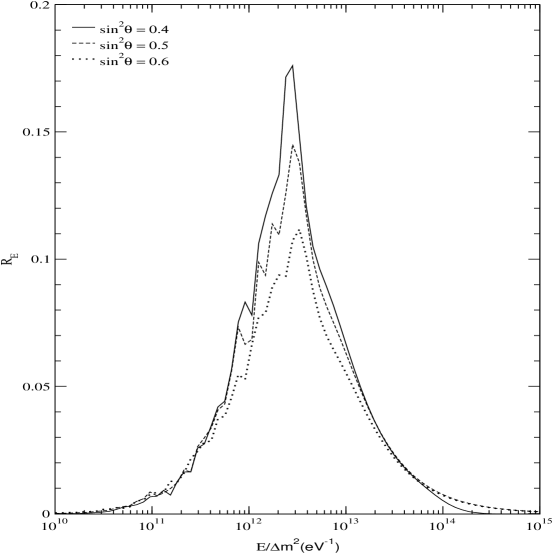
Figure 3.4: Earth regeneration of ${\nu_{e}}$ as a function of $\frac{E}{\mbox{$\Delta{m}^{2}$~{}}}$ for three different values of the mixing angle.

In fig 3.4 we show the Earth regeneration $R_{E}$ as a function of $\frac{E}{\mbox{$\Delta{m}^{2}$~{}}}$ for three values of the mixing angle in the range $0<\theta<\frac{\pi}{2}$. We note that the Earth matter effects are important only for $10^{11}$ eV${}^{-1}\stackrel{{\scriptstyle<}}{{\sim}}\frac{E}{\mbox{$\Delta{m}^{2}$~{}}}\stackrel{{\scriptstyle<}}{{\sim}}10^{14}$ eV^-1 which is the “pure” MSW regime and peaks at $\frac{E}{\mbox{$\Delta{m}^{2}$~{}}}\sim 3\times 10^{12}$ eV^-1. Since around $E=5-15$ MeV the SK day-night data allows for very small day-night asymmetry, most of regions around $(2-8)\times 10^{-6}$ eV² for large mixing angles are disfavored. In fig 3.5 we show the regeneration factor ${\rm f_{reg}}$ and the total Earth regeneration $R_{E}$ vs energy at the SK latitude for typical values of the parameters in the SMA, LMA and LOW-QVO regimes. Since the latitude of the other detectors are not very different we do not expect $f_{reg}$ and $R_{E}$ to be very different for them. Noteworthy point is that while the regeneration factor ${\rm f_{reg}}$ is positive for all the three cases considered, $R_{E}$ turns out to be negative for the SMA case. This is because for the SMA solution $P_{J}>1/2$, or in other words $P_{e2}^{\odot}-P_{e1}^{\odot}<1$, signifying large level crossing from the $\nu_{2}$ to the $\nu_{1}$ state in the solar matter at resonance. On the other hand for the LMA and LOW solutions the neutrino moves adiabatically inside the Sun, the ${\nu_{e}}$ produced in the $\nu_{2}$ state remains in a $\nu_{2}$ state throughout and $P_{e2}^{\odot}-P_{e1}^{\odot}\sim 1$, so that $R_{E}\approx{\rm f_{reg}}$. Thus for both LMA and LOW solutions one has positive regeneration of ${\nu_{e}}$ inside the Earth, the effect being more for the latter since for low $\Delta{m}^{2}$ all the neutrinos resonate far away from the production zone and $\cos 2\theta_{m}$ is closer to -1. Also note that for the LOW solution the regeneration is important at low energies while LMA has more regeneration for higher energy neutrinos.

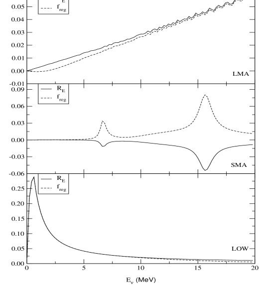
Figure 3.5: The regeneration factor ${\rm f_{reg}}$ and the net regeneration $R_{E}$ as a function of neutrino energy for typical values of the parameters in the SMA, LMA and LOW regions.

We finally present in fig 3.6 the actual survival probability $P_{ee}$ vs energy during day (shown by dotted lines), during night (shown by dashed lines) and the day-night average (shown by solid lines) for SMA, LMA and LOW case. In order to understand the nature of the probabilities we call $\cos 2\theta\equiv\epsilon$ and note that:

$\bullet$ For the SMA region $\epsilon\approx 1$ and from fig. 3.5 we observe that $f_{reg}$ is very small excepting for two peaks at E $\approx$ 6 MeV and E $\approx$ 15 MeV corresponding to strong enhancement of the earth regeneration effect for the neutrinos passing through the core [47, 42]. Hence

$$P_{ee}^{SMA}\approx P_{ee}^{D}$$ (3.46)

In this region for low energy ($pp$) neutrinos, resonance is not encountered (resonance density $\gg$ maximum solar density) and hence $P_{J}\approx 0$ and $\cos 2\theta_{m}\approx 1$ giving $P_{ee}^{SMA}\approx 1$. For intermediate energy (${}^{7}{Be}$) neutrinos $\cos 2\theta_{m}\approx-1$ (resonance density $\ll$ production density) and $P_{ee}^{SMA}\approx P_{J}\approx 0$ for these energies. For high energy (${}^{8}B$) neutrinos also, $\cos 2\theta_{m}\approx-1$ and $P_{ee}^{SMA}\approx P_{J}$, with $P_{J}$ rising with energy.

$\bullet$ For the LMA solution the motion of the neutrino in the solar matter is adiabatic for almost all neutrino energies and $P_{J}\approx 0$. For low energy neutrinos the matter effects are weak both inside the Sun and in Earth giving $f_{reg}\approx 0$ and $\cos 2\theta_{m}\approx\epsilon$ so that for Ga energies [48]

$$P_{ee}^{LMA}\approx\frac{1}{2}(1+\epsilon^{2})$$ (3.47)

At SK and SNO energies matter effects result in $\cos 2\theta_{m}\approx-1$ while $f_{reg}$ is small but non-zero ($\approx$ 0.03 at 10 MeV as seen from fig. 3.5) giving

$$P_{ee}^{LMA} \approx \frac{1}{2}(1-\epsilon)+f_{reg}$$ (3.48)

$$= \sin^{2}\theta+f_{reg}$$

$\bullet$ In the LOW region $\cos 2\theta_{m}\approx-1$ for all neutrino energies and $P_{J}\approx 0$ (except for very high energy neutrinos) and thus for all neutrino energies

$$P_{ee}^{LOW}=\frac{1}{2}(1-\epsilon)+f_{reg}$$ (3.49)

where $f_{reg}$ is small for high energy neutrinos and large for low energy neutrinos (cf. fig. 3.5).

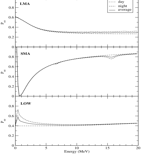
Figure 3.6: The neutrino survival probability $P_{ee}$ as a function of neutrino energy for the LMA, SMA and LOW solutions.

3.1.5 Results and Discussions

We present in Table 3.3 the results of the $\chi^{2}$ analysis for ${\nu_{e}}-\nu_{\rm active}$ oscillations, using data from the Cl, Ga, SK and SNO experiments. We use the total rates given in Table 3.2 and the 1258 day SK recoil electron energy spectrum at day and night. We show the best-fit values of the parameters $\Delta{m}^{2}$ and $\tan^{2}\theta$ , $\chi^{2}_{\rm min}$ and the goodness of fit (GOF) for the SMA, LMA, LOW-QVO, VO and Just So² [49] solutions.

The best-fit for the only rates analysis comes in the VO region which is favored at 28.79%. Prior to SNO the SMA solution could explain the nonmonotonic energy dependence of the survival probability from the Cl, Ga and SK experiments well and was the best-fit solution. But with the advent of SNO it falls into disfavor and is allowed at only 6.59%. For the LMA solution on the other hand the survival probability is given by eqs. (3.47) and (3.48) at Ga and SK/SNO energies respectively and for the values of $\epsilon$ from Table 3.3 and $f_{\rm reg}$ given in fig. 3.5, it approximately reproduces the rates of Table 3.2. LMA is allowed at 18.27% while LOW-QVO is barely allowed at 1.55%. In fact the LOW solution gets allowed only due to the strong Earth regeneration effects at low energies which helps the LOW solution to explain the Ga data better. In addition to these four solutions we have a fifth solution called the Just So² solution [49] at $\mbox{$\Delta{m}^{2}$~{}}\sim 5.38\times 10^{-12}$ eV². For these $\Delta{m}^{2}$ one gets a very small survival probability for the ${}^{7}{Be}$ neutrinos while for the ${}^{8}{B}~{}$neutrinos the survival probability is close to 1.0 [50]. Therefore it cannot explain the total rates data.

	Nature of	$\Delta m^{2}$	$\tan^{2}\theta$	$\chi^{2}_{min}$	Goodness
	Solution	in eV2			of fit
	SMA	$7.71\times 10^{-6}$	$1.44\times 10^{-3}$	5.44	6.59%
	LMA	$2.59\times 10^{-5}$	0.34	3.40	18.27%
rates	LOW-QVO	$1.46\times 10^{-7}$	0.67	8.34	1.55%
	VO	$7.73\times 10^{-11}$	0.27	2.49	28.79%
	Just So2	$5.38\times 10^{-12}$	1.29	19.26	$6.57\times 10^{-3}$%
	SMA	$5.28\times 10^{-6}$	$3.75\times 10^{-4}$	51.14	9.22%
rates	LMA	$4.70\times 10^{-5}$	0.38	33.42	72.18%
+	LOW-QVO	$1.76\times 10^{-7}$	0.67	39.00	46.99%
spectrum	VO	$4.64\times 10^{-10}$	0.57	38.28	50.25%
	Just So2	$5.37\times 10^{-12}$	0.77	51.90	8.10%

Table 3.3: The best-fit values of the parameters, $\chi^{2}_{\rm min}$ , and the goodness of fit from the global analysis of rates and rates+spectrum data for MSW oscillations involving two active neutrino flavors.

We next perform a complete global analysis of the solar neutrino data taking the four total rates and the 1258 day SK day-night recoil electron spectrum data. We present in Table 3.3 the results obtained by minimizing $\chi^{2}=\chi^{2}_{R}+\chi^{2}_{S}$. We get five allowed solutions LMA, VO, LOW, SMA and Just So² in order of decreasing GOF. The LMA solution can approximately reproduce the rates as discussed above and since the survival probability (3.48) for SK is approximately energy independent it can account for the flat recoil electron energy spectrum. LMA thus gives the best-fit being allowed at 72.18%. The LOW solution with best-fit $\epsilon=0.2$ and $f_{reg}\sim 0.2$ for Ga and $\sim 0.025$ for SK energies (cf. fig. 3.5) can just about reconcile the Ga and SK rates. However it provides a very good description of the flat SK spectrum and is allowed at 46.99%. The VO solution at $\mbox{$\Delta{m}^{2}$~{}}\sim 4.64\times 10^{-10}$ eV² gives a very low $\chi^{2}$ for the spectrum data and hence the overall fit for VO is very good. However for the SMA solution there is a mismatch between the parameters that give the minimum $\chi^{2}$ for the rates data and the spectrum data. The spectrum data prefers value of $\tan^{2}\theta$ which are one order of magnitude lower than those preferred by the rates data. Thus the overall fit in the SMA region suffers and it is allowed at only 9.22%. The Just So² solution is very bad for the rates but since it gives a flat probability for the ${}^{8}{B}~{}$neutrinos the spectrum shape can be accounted for and the global analysis gives a GOF of 8.1%.

In fig. 3.7 we show the 90%, 95%, 99% and 99.73% C.L. allowed areas from the analysis of the data on total rates (shown in the left hand panel) and the combined data on rates and the SK spectrum (shown in the right hand panel). For the only rates case we have allowed areas in the SMA, LMA, LOW-QVO and VO regions. For the global analysis we get allowed zones in the LMA and the LOW-QVO zones. In the VO region we get just two small areas which are allowed. But the most significant feature is the disappearance of the SMA solution from the global fit even at 99.73% C.L. ($3\sigma$).

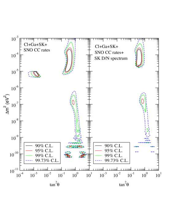
Figure 3.7: The 90%, 95%, 99% and 99.73% C.L. allowed areas from the analysis of the total rates (left panel) and global analysis of the rates and the 1258 day SK recoil electron spectrum at day and night (right panel), assuming MSW conversions to sequential neutrinos.

We have repeated the entire analysis for the ${\nu_{e}}-\nu_{\rm sterile}$ case and have reported the results of the fit in Table 3.4. We find that after the inclusion of the SNO data, all the solutions are disfavored with a probability of more than 99% from the total rates analysis while for the global analysis the GOF of these become much worse.

	Nature of	$\Delta m^{2}$	$\tan^{2}\theta$	$\chi^{2}_{min}$	Goodness
	Solution	in eV2			of fit
	SMA	$4.18\times 10^{-6}$	$5.72\times 10^{-4}$	17.24	$1.80\times 10^{-2}$ %
	LMA	$4.98\times 10^{-5}$	0.54	23.96	6.27$\times 10^{-4}$%
rates	LOW-QVO	$1.00\times 10^{-7}$	0.94	24.26	5.40$\times 10^{-4}$%
	VO	$1.07\times 10^{-10}$	0.27	15.71	$3.88\times 10^{-2}$%
	Just So2	$5.37\times 10^{-12}$	1.28	19.40	$6.13\times 10^{-3}$%
	SMA	5.59 $\times 10^{-6}$	$2.83\times 10^{-4}$	54.21	5.35%
rates	LMA	$6.13\times 10^{-5}$	0.50	52.93	6.75%
+	LOW-QVO	$2.93\times 10^{-8}$	1.00	53.18	6.45%
spectrum	VO	$4.67\times 10^{-10}$	0.37	46.28	19.70%
	Just So2	$5.37\times 10^{-12}$	0.77	52.09	7.83%

Table 3.4: The best-fit values of the parameters, $\chi^{2}_{\rm min}$ , and the goodness of fit from the global analysis of rates and rates+spectrum data for MSW oscillations involving ${\nu_{e}}-\nu_{\rm sterile}$ oscillations.

3.2 The Atmospheric Neutrino Anomaly

The atmospheric neutrinos are produced due to the collision of cosmic rays ($N_{cr}$) with the nuclei in the atmosphere ($N_{air}$) resulting in a chain of reactions which culminates in the production of neutrinos and antineutrinos with expected flavor ratio of roughly ${\nu_{e}}:{\nu_{\mu}}:{\nu_{\tau}}\approx 1:2:0$.

$$N_{cr}+N_{air} \longrightarrow \pi^{\pm},~{}K^{\pm},~{}K^{0},......$$ (3.50)

$$\pi^{\pm}(~{}K^{\pm}) \longrightarrow \mu^{\pm}+{\nu_{\mu}}({\bar{\nu}_{\mu}})$$

$$\mu^{\pm} \longrightarrow e^{\pm}+{\nu_{e}}({\bar{\nu}_{e}})+{\bar{\nu}_{\mu}}({\nu_{\mu}})$$ (3.51)

The first pioneering measurement of events induced by these neutrinos were made in the Kolar Gold Fields in India [51] and almost simultaneously in South Africa [52]. But the interpretation of the results from these experiments remained ambiguous due to both theoretical as well as experimental uncertainties. It was only since late eighties that people earnestly started pursuing this problem [53, 54, 55, 56, 57, 58] and around 1988 Kamiokande, which was originally designed to detect proton decay, declared its results on atmospheric neutrino measurements which showed a marked deficit of observed to expected ${\nu_{\mu}}/{\nu_{e}}$ ratio [53]. This embodies the Atmospheric Neutrino Anomaly. This was the second evidence of missing neutrinos after the solar neutrino problem and again called for the existence of neutrino mass and mixing for the correct interpretation of the experimental results.

However due to the large theoretical and experimental uncertainties involved in the atmospheric neutrino measurement, it failed to prove itself as a compelling evidence of neutrino oscillations until the arrival of the Super-Kamiokande atmospheric results in 1998 [58]. The SK atmospheric neutrino data [58, 59, 60] not only confirmed the suppression of the muon type neutrinos, it also firmly established the fact that the observed deficit has a zenith angle dependence. That is, the neutrinos coming at larger zenith angles and hence traveling distances of the order of the diameter of the Earth were suppressed more compared to neutrinos arriving directly from the top of the detector. This differential depletion of the atmospheric ${\nu_{\mu}}$ flux is referred to as the observed up-down asymmetry. The ${\nu_{e}}$ events on the other hand are reported to be consistent with theoretical expectations.

The most convincing particle physics scenario which can explain all aspects of the SK data is ${\nu_{\mu}}-{\nu_{\tau}}$ oscillations with $\mbox{$\Delta{m}^{2}$~{}}\sim 10^{-3}$ eV² and $\mbox{$\sin^{2}2\theta$~{}}\sim 1$ [61, 62, 63, 64]. Thus the theory of neutrino mass and mixing, which was conjectured in the late sixties as a plausible solution to the solar neutrino problem, was established as an accepted reality by the SK atmospheric neutrino results in 1998. This observation of neutrino mass by the SK (although indirect) is the first and till date the only evidence of physics beyond the standard model of particle physics.

The observed depletion of atmospheric neutrinos was also reported by the IMB [55] earlier and more recently by the Soudan2 [65] and MACRO [66] collaborations. In order to do justice to all these experiments one should perform a global analysis taking all the experimental data into account. However due to its overwhelming statistics, the SK data dictates the atmospheric neutrino analysis, with the other experiments having little impact on the fit and the allowed parameter regions. Hence considering the rich statistics and low systematics of the SK, we choose to work with just the SK data in our analysis of the atmospheric neutrino anomaly and perform dedicated $\chi^{2}$ -fits to the SK 1144 day data. We describe two different established methods of $\chi^{2}$ analysis of the atmospheric data and discuss their merits and demerits, present the best-fit $\Delta{m}^{2}$ and $\sin^{2}2\theta$ and display the 90% and 99% C.L. allowed zones in the $\Delta{m}^{2}$ -$\sin^{2}2\theta$ parameter space for two-generation ${\nu_{\mu}}-{\nu_{\tau}}$ oscillations.

In section 3.2.1 we give an essence of the atmospheric neutrino flux calculations and the theoretical uncertainties associated with it. In section 3.2.2 we discuss the various features of the SK atmospheric experiment and state the main experimental results. In section 3.2.3 we describe our atmospheric neutrino code and discuss the advantages and disadvantages of the two methods of $\chi^{2}$ analysis that we have used. Finally in section 3.2.4 we present the results of our $\chi^{2}$ fits.

3.2.1 Atmospheric Neutrino Flux Predictions

Atmospheric neutrinos are the result of a cascade of reactions following the interaction of the cosmic rays with the air nuclei (cf. eq. (3.50), (3.51)). In the decay chain (3.51), for every electron neutrino (or antineutrino) created one has two muon type neutrinos (or antineutrinos) produced. Thus one may naively guess that the ratio of fluxes

$${\cal R} = \frac{{\nu_{\mu}}+{\bar{\nu}_{\mu}}}{{\nu_{e}}+{\bar{\nu}_{e}}}$$ (3.52)

$$\approx 2$$

But for a realistic prediction for the atmospheric neutrino fluxes one needs to fold in the cosmic ray fluxes with the hadronic interaction model, which takes into account the complete reaction chain and perform a comprehensive calculation. Two such widely used atmospheric flux calculations are by Honda et al.[67] and Agarwal et al.[68].

The primary cosmic rays which are the main ingredient of the atmospheric neutrino flux calculations have large uncertainties in their over all normalization, composition, as well as in their spectrum, all of which are extremely crucial in the atmospheric neutrino flux calculations. Though the cosmic ray fluxes are relatively well known at $E\stackrel{{\scriptstyle<}}{{\sim}}30$ GeV (these give rise to the sub-GeV atmospheric neutrino fluxes), there are few experimental measurements for the higher energy cosmic rays ($E\stackrel{{\scriptstyle<}}{{\sim}}1000$ GeV which result in multi-GeV neutrino fluxes) and hence this regime is plagued with large uncertainties.

The resultant atmospheric neutrino fluxes also depend crucially on the hadronic interaction model. In their calculation, Honda et al.use a full Monte Carlo method for the sub-GeV neutrinos while for the multi-GeV fluxes they employ a “hybrid model” [67]. They make their atmospheric neutrino flux calculations using a one-dimensional approximation where they assume that all the secondary particles including the mesons and the leptons are collinear with the incident primary cosmic ray. Though this approximation works well for the higher energy calculations, it fails for the low energy sub-GeV fluxes, particularly for the horizontal zenith angles and therefore should be replaced by a full three-dimensional calculation[69].

Let us next discuss some of the most important factors which affect the atmospheric neutrino flux predictions.

1. The solar activity: The effect of the solar wind on the cosmic rays entering the solar sphere of influence is to deviate their trajectories away from the Earth. This affects the low energy cosmic rays more than the higher energy ones and is known as the solar modulation of the cosmic ray fluxes. Since the solar wind depends on the solar activity, the fluxes are maximum at the solar minimum and minimum at the solar maximum.

2. The geomagnetic field: Since the cosmic rays consist of charged particles they experience a repulsion due to the Earth’s magnetic field and may be deflected away. Hence only particles with momentum above a certain threshold can break this barrier and enter the Earth’s atmosphere. This threshold is called the rigidity cut off and is defined as, rigidity=momentum/charge. This effect results in cutting off the lower energy cosmic rays which affects the low energy neutrino fluxes. The geomagnetic field bends the cosmic rays and thus introduces a directionality into the atmospheric fluxes, the effect obviously being more for lower energy neutrinos. This effect of the geomagnetic field results in predicting more neutrino flux from the west than from the east and is known as the east-west effect. SK has made observations of this predicted east-west anisotropy and has confirmed this estimated directional behavior [70].

3. The density structure of the atmosphere: Once the pions and kaons are produced in the air, they may either decay creating muons and neutrinos or may interact with other particles. Which of these processes dominate is dictated by the energy of the meson and decay becomes comparable to interaction when

   $${\rm c}\frac{E}{{\rm mc}^{2}}\tau\sim\frac{1}{\sigma n},~{}~{}{\rm or}~{}~{}E\sim\frac{{\rm mc}^{2}}{{\rm c}\tau\sigma n}$$ (3.53)

   where $\tau$ is the rest frame lifetime of the meson of energy $E$ and mass m, $\sigma$ is the interaction cross-section with air and $n$ is the number density of the air nuclei. Since the interaction rate depends inversely on the density of the atmosphere, and since the cosmic rays moving along the horizontal zenith angle interact with the air nuclei at a higher altitude (and hence lower density), the decay probability for these is more compared to interaction. Hence the resultant neutrino fluxes are maximum along the horizontal and minimum along the vertical directions. This gives rise to the zenith angle variation of the neutrino flux. Again, because the interaction rate of the meson is determined by its energy, the zenith angle dependence of the neutrino flux increases with energy.

4. Decay lifetime of the mesons: The ratio ${\cal R}\approx 2$ only for $\pi$ decays at rest for which the decay (3.51) is complete. However above $E\stackrel{{\scriptstyle>}}{{\sim}}5$ GeV the decay lifetime of the produced muon becomes so large that they fail to decay in air. This results in raising the value of ${\cal R}$ from 2. Again, as the effective atmospheric depth along the horizontal direction is more than that along the vertical, the decay chain (3.51) has comparatively a better chance of completion along the horizontal direction and this results in endowing ${\cal R}$ with a zenith angle dependence.

Though the uncertainty due to primary cosmic rays for the sub-GeV neutrinos is small, they are significantly modulated by the solar activity and the geomagnetic field. Being low in energy, they have less zenith angle dependence. The multi-GeV fluxes on the other hand have less dependence on solar activity and geomagnetic field, but have large zenith angle variation and have to contend with huge cosmic ray uncertainties. We show in fig 3.8 the atmospheric neutrino flux predictions by Honda et al.[67] as a function of the zenith angle for three typical values of energies. Also shown in the lower panels are the corresponding values of ${\cal R}$. The fluxes shown are without the geomagnetic effects so that they are symmetric about the horizontal and hence the sign of $\cos\xi$ is not important. We note that both ${\nu_{e}}$ as well as ${\nu_{\mu}}$ decrease along the vertical, displaying the zenith angle behavior discussed above, the effect being more for the ${\nu_{e}}$. Thus the ratio ${\cal R}$ gets raised from the often quoted value of 2 along the vertical. The above effect is seen to intensify with energy.

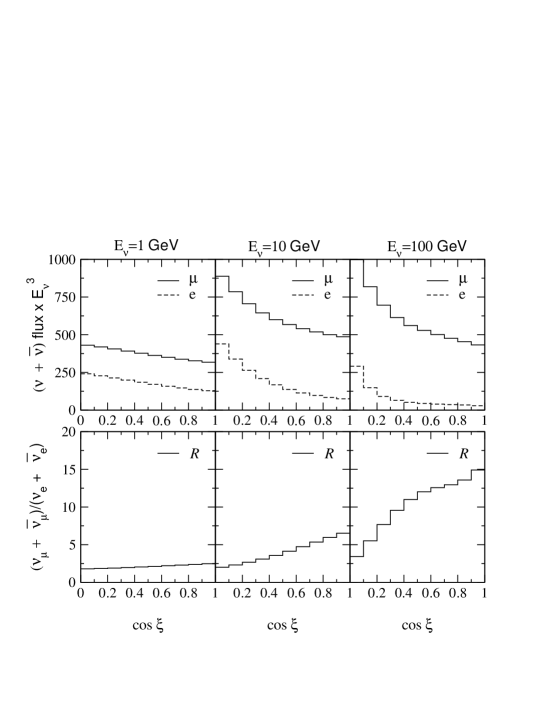
Figure 3.8: The atmospheric neutrino fluxes as a function of the neutrino zenith angle for three different fixed energies. Shown are the absolute fluxes as well as the ratio ${\cal R}$.

Among the major uncertainties involved in the atmospheric flux calculations, the most important contribution comes from the lack of correct estimates for the cosmic ray flux normalization, composition and spectrum. This results in about $10\%$ error in the sub-GeV fluxes and 20% error in the multi-GeV flux range. The hadronic interaction model brings about 10% uncertainty above 300 MeV. The other sources of uncertainties include the method of calculation employed and the use of one-dimensional approximation. All these factors sum up to result in total uncertainty of about 20–30% in the absolute values of the fluxes [67]. For the ratio ${\cal R}$ on the other hand the uncertainties due to the primary cosmic rays and the error in the calculation scheme cancel out and one has only about 5% error for the sub-GeV and about 10% error for the multi-GeV neutrinos [67].

3.2.2 Results from the Super-Kamiokande

The Super-Kamiokande as described before is a large water $\breve{\rm C}$erenkov detector. It contains 50 kton of ultra pure water, divided into two concentric cylinders. The inner detector with a fiducial volume of 22.5 ktons, has its surface lined by 11,146 inward facing 50cm photomultiplier tubes and 1885 outward facing 20cm photomultiplier tubes. The outward facing phototubes view the outer detector volume which serves both as a particle shield as well as a detector. The main process by which it detects the atmospheric neutrinos is the charged current quasi-elastic interaction

$$\nu_{l}+N\rightarrow l+N^{\prime}$$ (3.54)

where the flavor of the incident neutrino is tagged onto the flavor of the released lepton. As this lepton moves in water it emits a $\breve{\rm C}$erenkov cone which can be viewed by the phototubes lining the detector walls. The SK classifies its data into

• $e$ type or $\mu$ type events: The single-ring events can be classified into $e$ or $\mu$ type depending on whether the observed $\breve{\rm C}$erenkov ring is fuzzy or sharp respectively.

• contained events: Events for which the products of neutrino interaction are contained within the detector volume are called contained events. If the products are fully contained within the inner detector volume itself, then these events are termed fully-contained events (FC). On the other hand if the produced leptons exit the inner detector volume and stop in the outer detector, then these events are called partially-contained events (PC). Only muons are penetrating enough to be able enter the outer detector and so only ${\nu_{\mu}}$ have PC events.

• sub-GeV and multi-GeV events: Depending on the value of the visible energy of the released lepton ($E_{vis}$) the FC events are categorized as sub-GeV (if $E_{vis}<1.33$ GeV) or multi-GeV (if $E_{vis}>1.33$ GeV).

• upward-going muons: If the muons are produced in the rock below the detector and penetrate into the detector volume, then such events are grouped together to be called upward-going muons [71]. If these muons traverse the entire detector volume and escape out then they are termed as upward through-going muons. If on the other hand they stop within the detector then one has upward stopping muons. These upward-going muons are recorded for zenith angle $>90^{o}$ only. The neutrino induced muons with zenith angle less than this are not taken into account due the huge contamination resulting from the muons in the cosmic ray fluxes themselves.

• zenith angle bins: At the detector, the neutrino flux come from all directions. Thus, the total path length between the production point in the atmosphere and the detector varies from about 10 km to 13,000 km depending on the zenith angle. Neutrinos with zenith angle less than $90^{\rm o}$ (downward neutrinos) travel a distance of $\sim$ 10 – 100 km from their production point in the atmosphere to the detector while the neutrinos with larger zenith angles (upward neutrinos) cross a distance of up to $\sim$ 13,000 km to reach the detector. The SK can see the zenith angle of the lepton that emits the $\breve{\rm C}$erenkov cone. The lepton zenith angle $\Theta$ is related to the incoming neutrino zenith angle $\xi$ through the relation

  $$\cos\Theta=\cos\xi\cos\psi+\sin\xi\cos\phi\sin\psi$$ (3.55)

  where $\psi$ is the angle between the incoming neutrino $\nu_{l}$ and the scattered lepton $l$ and $\phi$ is the azimuthal angle corresponding to the incident neutrino direction. The SK divides its events into bins corresponding to the zenith angle of the observed lepton $\cos\Theta$.

After 1144 day of data taking [72] the SK divide their observed number of sub-GeV and multi-GeV $e$ type and $\mu$ type events into 10 zenith angle bins each. Instead of showing the actual number of events reported by SK, for the sake of clarity we present in fig 3.9 the ratio of the number of observed ($N$) to the number of expected ($N_{0}$) events, for the sub-GeV $e$-type (${\rm SG_{e}}$ ), multi-GeV $e$-type (${\rm MG_{e}}$ ), sub-GeV $\mu$-type (${\rm SG_{\mu}}$ ) and multi-GeV $\mu$-type (${\rm MG_{\mu}}$ ) data samples. We have included the PC events along with the FC ${\rm MG_{\mu}}$ events in the panel for ${\rm MG_{\mu}}$ . Henceforth we will follow this procedure for representation of the PC and ${\rm MG_{\mu}}$ data samples. The ratio $N/N_{0}$ are shown for the ten zenith angle bins along with the $\pm 1\sigma$ errorbars.

Figure 3.9: The sub-GeV and multi-GeV event distributions vs. zenith angle. $N$ is the number of observed $e$ type or $\mu$ type events and $N_{0}$ is the Monte Carlo expectation. The errorbars show the $\pm 1\sigma$ uncertainties. Also shown by the dashed lines are the zenith angle distributions for the various data samples predicted by the two-generation ${\nu_{\mu}}-{\nu_{\tau}}$ oscillation best-fit solution.

Had there been no anomaly this ratio would have been one for all the data bins. However we observe that

1. The $e$-type events, both ${\rm SG_{e}}$ and ${\rm MG_{e}}$ , are consistent with theoretical expectations.

2. The observed $\mu$-type events on the other hand show depletion compared to expectations.

3. The deficit of $\mu$-type events has a zenith angle distribution. The ${\nu_{\mu}}$ depletion being most in the first zenith angle bin (upward) and least in the last one (downward), for both the ${\rm SG_{\mu}}$ and ${\rm MG_{\mu}}$ data samples. Thus the data has a marked up-down asymmetry.

4. In addition the ${\nu_{\mu}}$ deficit has an energy dependence. The up-down asymmetry being more for the multi-GeV than for the sub-GeV neutrinos.

Since the uncertainties in the absolute fluxes are immense ($\approx 30\%$), one may instead use the double ratio,

$$R=\frac{(N_{\mu}/N_{e})|_{\rm obs}}{(N_{\mu}/N_{e})|_{MC}}$$ (3.56)

where $(N_{\mu}/N_{e})|_{\rm obs}$ are the ratio of the total number of observed $\mu$-type to $e$-type events in the detector and $(N_{\mu}/N_{e})|_{MC}$ is the corresponding Monte Carlo expectation. Different atmospheric flux calculations agree to within better than 5% on the magnitude of this quantity. The up-down asymmetry can be then expressed in terms of an up-down asymmetry parameter $Y_{l}$ defined as [64]

$$Y_{l}\equiv{(N_{l}^{-0.2}/N_{l}^{+0.2})|_{obs}\over(N_{l}^{-0.2}/N_{l}^{+0.2})|_{MC}}$$ (3.57)

Here $N_{l}^{-0.2}$ denotes the number of $l$-type events produced in the detector with zenith angle $\cos\Theta<-0.2$, i.e. the upward neutrino events while $N_{l}^{+0.2}$ denotes the number of $l$-type events for $\cos\Theta>0.2$ i.e. events coming from downward neutrinos. The central bin has contributions from both upward and downward neutrinos and is not useful for studying the up-down asymmetry. For the 848 day and 535 day data the $R$ and $Y_{l}$ are given in Table 3.5. The $Y_{e}$ is close to 1 but the $Y_{\mu}$ and $R$ are less than unity for both the sub-GeV as well multi-GeV cases.

	848   day   data		535   day   data
Quantity	Sub-GeV	Multi-GeV	Sub-GeV	Multi-GeV
$R$	$0.69\pm 0.05$	$0.68\pm 0.09$	$0.63\pm 0.06$	$0.65\pm 0.09$
$Y_{\mu}$	$0.74\pm 0.04$	$0.53\pm 0.05$	$0.76\pm 0.05$	$0.55\pm 0.06$
$Y_{e}$	$1.03\pm 0.06$	$0.95\pm 0.11$	$1.14\pm 0.08$	$0.91\pm 0.13$

Table 3.5: The double ratio $R$ and up-down asymmetry parameter $Y_{l}$.

3.2.3 The Atmospheric Neutrino Code

The expected number of $l$ (e or $\mu$) like 1 ring events recorded in the detector in presence of oscillations is given by

$$N_{l} = n_{T}\int^{\infty}_{0}dE\int^{(E_{l})_{\rm max}}_{(E_{l})_{\rm min}}dE_{l}\int_{-1}^{+1}d\cos\psi\int_{-1}^{+1}d\cos\xi\ {1\over 2\pi}\int_{0}^{2\pi}d\phi$$ (3.58)

$$\times {d^{2}F_{l}(E,\xi)\over dE~{}d\cos\xi}\cdot{d^{2}\sigma_{l}(E,E_{l},\cos\psi)\over dE_{l}~{}d\cos\psi}\epsilon(E_{l})\cdot{\ }P_{\nu_{l}\nu_{l}}(E,\xi).$$

where $n_{T}$ denotes the number of target nucleons, $E$ is the neutrino energy, $E_{l}$ is the energy of the final charged lepton, $\psi$ is the angle between the incoming neutrino $\nu_{l}$ and the scattered lepton $l$, $\xi$ is the zenith angle of the neutrino and $\phi$ is the azimuthal angle corresponding to the incident neutrino direction (the azimuthal angle relative to the $\psi$ has been integrated out). The zenith angle of the charged lepton in terms of $\psi$, $\xi$ and $\phi$ is given by eq. (3.55). $d^{2}F_{l}/dEd\cos\xi$ is the differential flux of atmospheric neutrinos of type $\nu_{l}$, $d^{2}\sigma_{l}/dE_{l}d\cos\psi$ is the differential cross section for $\nu_{l}N\rightarrow lX$ scattering and $\epsilon(E_{l})$ is the detection efficiency for the 1 ring events in the detector. The efficiencies that were available to us are not the detection efficiencies of the charged leptons but some function which we call $\epsilon^{\prime}(E)$ defined as [73]

$$\epsilon^{\prime}(E)=\frac{\int{\frac{d\sigma}{dE_{l}}\epsilon(E_{l})dE_{l}}}{\int{\frac{d\sigma}{dE_{l}}dE_{l}}}$$ (3.59)

$P_{\nu_{l}\nu_{l}}$ is the survival probability of a neutrino flavor $l$ after traveling a distance $L$ given by,

$$L=\sqrt{(R_{e}+h)^{2}-{R_{e}}^{2}\sin^{2}\xi}-R_{e}\cos\xi$$ (3.60)

$R_{e}$ being the radius of the Earth and $h$ is the height of the atmosphere where the neutrinos are produced. We use the atmospheric neutrino fluxes from [67]. For the sub-GeV events the dominant process is the charged current quasi-elastic scattering from free or bound nucleons. We use the cross-sections given in [74]. The events in multi-GeV range have contributions coming from quasi-elastic scattering, single pion production and multi pion production and we have used the cross-sections given in [75]. For the multi-GeV events we assume that the lepton direction $\Theta$ is the same as the incoming neutrino direction $\xi$. But actually they are slightly different. We simulate this difference in the zenith angles by smearing the angular distribution of the number of events with a Gaussian distribution having a one sigma width of $15^{\rm o}$ for $\mu$ type events and $25^{\rm o}$ for the $e$ type events [63]. For the sub-GeV events, difference in direction between the charged lepton and the neutrinos are exactly taken care of according to eq. (3.58) and (3.55).

In order to do a statistical analysis of the data we define a $\chi^{2}$ function as [64]

$$\chi^{2}=\sum_{i}\left[\left({R}^{exp}-R^{th}\over\Delta R^{exp}\right)^{2}+\left({Y^{exp}_{\mu}-Y^{th}_{\mu}\over\Delta Y^{exp}_{\mu}}\right)^{2}+\left({Y^{exp}_{e}-Y^{th}_{e}\over\Delta Y^{exp}_{e}}\right)^{2}\right]$$ (3.61)

where the sum is over the sub-GeV and multi-GeV cases. The experimentally observed rates are denoted by the superscript “exp” and the theoretical predictions for the quantities are labeled by “th”. $\Delta R^{exp}$ is the error in $R$ obtained by combining the statistical and systematic errors in quadrature. $\Delta Y^{exp}$ corresponds to the error in $Y$. For this we take only the statistical errors since these are much larger compared to the systematic errors. We include both the $e$-like and the $\mu$-like up-down asymmetries in the fit so that we have 4 degrees of freedom (6 experimental data - 2 parameters) for the oscillation analysis in the two parameters $\Delta m^{2}$ and $\sin^{2}2\theta$.

The use of these type of ratios for the $\chi^{2}$ analysis test has been questioned in [76] because the error distribution of these ratios is non-Gaussian in nature. However as it has been shown in [64] the use of the $R$’s and $Y$’s as defined above is justified within the 3$\sigma$ region around the best-fit point for a high statistics experiment like SK and provides an alternative way of doing the $\chi^{2}$-analysis. A comparison of the results of [64] with those obtained in [63, 61] shows that the best-fit points and the allowed regions obtained do not differ significantly in the two approaches of data fitting. The advantage of using the ratios is that they are relatively insensitive to the uncertainties in the neutrino fluxes and cross-sections as the overall normalization factor gets canceled out in the ratio. We have included the $Y_{e}$ in our analysis because to justify the $\nu_{\mu}-\nu_{\tau}$ oscillation scenario, it is necessary to check that $\chi^{2}$ including the data on electron events gives a low value and hence it is the standard practice to include these in the $\chi^{2}$-analysis [64, 63, 61].

Even though the method of $\chi^{2}$ analysis defined above is acceptable, a better method is to use the absolute number of e or $\mu$ type events taking into account the errors and their correlations properly [61, 63]. Following this method we define our $\chi^{2}$ as [61, 63]

$$\chi^{2}=\sum_{i,j=1,40}\left(N_{i}^{th}-N_{i}^{exp}\right)(\sigma_{ij}^{2})^{-1}\left(N_{j}^{th}-N_{j}^{exp}\right)$$ (3.62)

where the sum is over the sub-GeV and multi-GeV electron and muon bins. The experimentally observed number of events are denoted by the superscript “exp” and the theoretical predictions for the quantities are labeled by “th”. The element of the error matrix $\sigma_{ij}$ is calculated as in [61], including the correlations between the different bins. For two-generation analysis of the SK atmospheric neutrino data we employ this second more widely used method of $\chi^{2}$ analysis and present our results in the next section.

3.2.4 Results and Discussions

Since the $e$ type events are consistent with the Monte Carlo expectations, the only possible two-generation oscillation schemes that one should consider to be responsible for the ${\nu_{\mu}}$ deficit are the ${\nu_{\mu}}-{\nu_{\tau}}$ and ${\nu_{\mu}}-\nu_{\rm sterile}$ oscillation modes. The two cases differ from each other in the Earth matter effects on the mass and mixing parameters for the upward neutrinos. While for ${\nu_{\mu}}-{\nu_{\tau}}$ oscillations there are no effects of the Earth matter, the ${\nu_{\mu}}-\nu_{\rm sterile}$ has its $\Delta{m}^{2}$ and $\sin^{2}2\theta$ modulated in presence of matter since the sterile neutrinos do not have any interaction with the ambient matter. For the ${\nu_{\mu}}-\nu_{\rm sterile}$ case the mass squared difference and mixing angle in matter are given by eq. (2.52) and eq. (2.53) of chapter 2. Since for the atmospheric neutrino anomaly the mixing angle in vacuum is close to maximal, the effect of matter in this case is mostly to reduce the mixing. Thus the ${\nu_{\mu}}-\nu_{\rm sterile}$ oscillations predict a lower suppression of the upward neutrinos than demanded by the data and fail to reproduce the correct zenith angle distribution, the effect being more for the higher energy neutrinos. Thus the ${\nu_{\mu}}-\nu_{\rm sterile}$ solution gets disfavored by the zenith angle data. In addition, since the sterile neutrinos do not induce any neutral current event in the detector while both the $\mu$ and $\tau$ neutrinos do, for ${\nu_{\mu}}-\nu_{\rm sterile}$ mixing one expects a reduction of the neutral current events while for ${\nu_{\mu}}-{\nu_{\tau}}$ oscillations they remain unchanged. In their paper [77], the SK collaboration have shown that their neutral current sample is consistent with expectations, there is no depletion of the events and hence transition of ${\nu_{\mu}}$ to $\nu_{\rm sterile}$ are disfavored. The SK collaboration have given 99% C.L. exclusion plots for a combined analysis of the neutral current enriched multi-ring events, the high energy partially contained events and the upward-going muon data sets, in terms of ${\nu_{\mu}}-\nu_{\rm sterile}$ oscillations. They superimpose the 99% C.L. allowed region that they obtain from the $\chi^{2}$ analysis of the FC data over these exclusion plots and show that there is no region of overlap between the two. They thus conclude that pure two-generation ${\nu_{\mu}}-\nu_{\rm sterile}$ oscillations are disfavored by the data and hence the pure ${\nu_{\mu}}-{\nu_{\tau}}$ mixing, which can provide excellent fit to all the atmospheric data samples without any inconsistency is the favored alternative [77]. The latest 1289 day data sample on the upward-going events are consistent with ${\nu_{\tau}}$ appearance at the $2\sigma$ level [78] thereby further disfavoring the sterile option. We therefore concentrate on the ${\nu_{\mu}}-{\nu_{\tau}}$ oscillation scenario.

In the two-flavor ${\nu_{\mu}}-{\nu_{\tau}}$ picture the survival probability of an initial $\nu_{\mu}$ of energy $E$ after traveling a distance $L$ in vacuum is

$$P_{\nu_{\mu}\nu_{\mu}}=1-\sin{{}^{2}}2\theta\sin{{}^{2}}(\pi L/\lambda_{osc})$$ (3.63)

where $\theta$ is the mixing angle between the two neutrino states in vacuum and $\lambda_{osc}$ is the oscillation wavelength defined as,

$$\lambda_{osc}=(2.47~{}km)~{}\frac{E}{GeV}\frac{eV^{2}}{\Delta m^{2}}$$ (3.64)

where $\Delta m^{2}$ denotes the mass squared difference between the two mass eigenstates. If we insert eq. (3.63) in eq. (3.58) and minimize the $\chi^{2}$ function defined by (3.62), then for the 1144 day of SK data we get the following best-fits and $\chi^{2}_{\rm min}$

• $\chi^{2}_{min}=36.23$, $\Delta m^{2}$ = 0.0027 eV², $\sin^{2}2\theta$ = 1.0

For 38 degrees of freedom ($40-2$) this corresponds to a goodness of fit of 55.14%. We present in fig. 3.10 the 90% and 99% C.L. allowed area in the neutrino parameter space for two-generation ${\nu_{\mu}}-{\nu_{\tau}}$ oscillations. In fig 3.9 we show with dashed lines the histograms for the best-fit value for two-generation ${\nu_{\mu}}-{\nu_{\tau}}$ oscillations. Both the absolute number of events as well as the zenith angle distributions of the SK data are seen to be reproduced well.

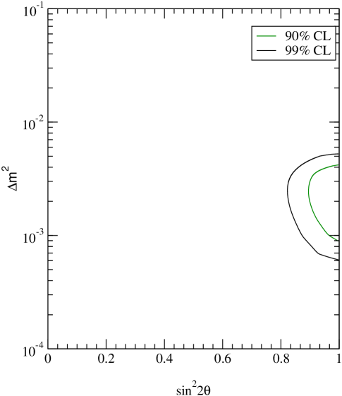
Figure 3.10: Region of the parameter space allowed by the ${\nu_{\mu}}-{\nu_{\tau}}$ oscillation solution to the 1144 day SK atmospheric neutrino data. Shown are the 90% and 99% C.L. allowed zones.

3.3 Bounds from Accelerator and Reactor Experiments

Neutrino oscillations experiments can be broadly classified into two types:
$\bullet$ Disappearance experiments: In these one starts with a neutrino beam of a definite flavor $\nu_{\alpha}$ and looks for a reduction in the original flux, after the beam has traveled a certain distance.
$\bullet$ Appearance experiments: These experiments search for a new flavor $\nu_{\beta}$ in the original $\nu_{\alpha}$ beam, after it has been made to travel a distance L.

Both the solar neutrino problem and the atmospheric neutrino anomaly that we have discussed above are disappearance experiments. But both these experiments have the intrinsic defect of large uncertainties in model predictions of neutrino fluxes. The neutrino beams in the laboratory experiments on the other hand have well controlled spectrum as well as path length and hence are better suited for precise study of neutrino mass and mixing parameters. The laboratory accelerator and reactor experiments may operate in either the disappearance or appearance modes. While the appearance experiments have the advantage of being apparently easier, since one is looking for a new flavor absent in the initial beam, the disappearance experiments have the strength to probe the oscillations of the initial $\nu_{\alpha}$ to all channels including $\nu_{\alpha}-\nu_{\rm sterile}$ which can never be seen in an appearance experiments.

In two-generations the conversion probability of $\nu_{\alpha}$ to another flavor $\nu_{\beta}$ after traveling distance $L$ is given by eq. (2.11)

$$P_{\nu_{\alpha}\nu_{\beta}} = \sin^{2}2\theta\sin^{2}(\frac{\pi L}{\lambda})$$ (3.65)

$$= \sin^{2}2\theta\sin^{2}\left(1.27\frac{\mbox{$\Delta{m}^{2}$~{}}L}{E}\right)$$

$\lambda$ being the oscillation wavelength. Sensitivity of a given experiment can be ascertained in terms of the minimum $\Delta{m}^{2}$ and $\sin^{2}2\theta$ that the experiment can probe. For $\Delta{m}^{2}$ very large $\lambda\ll L$, and $\sin^{2}(\frac{\pi L}{\lambda})\rightarrow\frac{1}{2}$. For the limiting value of $P_{\nu_{\alpha}\nu_{\beta}}^{0}$ seen by the experiment

$$\sin^{2}2\theta_{\rm min}=2P_{\nu_{\alpha}\nu_{\beta}}^{0}$$ (3.66)

On the other hand if $\Delta{m}^{2}$ is such that $\left(\frac{\mbox{$\Delta{m}^{2}$~{}}L}{E}\right)$ is very small then we can replace the sine function by its argument.

$$P_{\nu_{\alpha}\nu_{\beta}}^{0}=\sin^{2}2\theta\left(1.27\frac{\mbox{$\Delta{m}^{2}$~{}}L}{E}\right)^{2}$$ (3.67)

Hence the minimum value of $\Delta{m}^{2}$ that the experiment can constraint corresponds to the case where $\mbox{$\sin^{2}2\theta$~{}}\rightarrow 1$, that is

$$\Delta m^{2}_{\rm min}=\frac{P_{\nu_{\alpha}\nu_{\beta}}^{0}}{1.27L/E}$$ (3.68)

Using the above argument the terrestrial experiments give exclusion plots in the $\Delta{m}^{2}$ –$\sin^{2}2\theta$ plane. All accelerator and reactor experiment till date barring the LSND in Los Alamos have failed to observe any positive signal of neutrino oscillations and give exclusion plots in the $\Delta{m}^{2}$ –$\sin^{2}2\theta$ plane. We give below a list of the most prominent experiments and their main features.

$\bullet$ Reactor Experiments
The neutrinos in these experiments are produced in $\beta$ decay of fission products in the reactors. Thus typically one has an initial ${\bar{\nu}_{e}}$ beam with energies of the order a few MeV. Since the energies are so small these experiments operate in the disappearance mode. These ${\bar{\nu}_{e}}$ are detected by liquid scintillation detectors through the reaction

$${\bar{\nu}_{e}}+p\rightarrow e^{+}+n$$ (3.69)

Since these are necessarily disappearance experiments, the incident neutrino flux should be very accurately known to reduce the systematic uncertainties. Due to these high systematic uncertainties the reactor experiments fail to probe very low values of $\sin^{2}2\theta$ . To overcome this problem to some extent and to reduce the uncertainties, most experiments use two or more detectors placed at different distances and what is used in the analysis is the ratio of the neutrino flux observed at these different detectors. The characteristics of the most important reactor experiments and their limits on the oscillation parameters are listed in Table 3.6. Among the reactor experiments the most stringent bounds in the low $\Delta{m}^{2}$ range are obtained from the CHOOZ long-baseline experiment in France [82]. This experiment has a baseline of 1 km so that it has an average $L/E\sim 3$ ($E\sim 3$ MeV) and hence is sensitive to $\Delta{m}^{2}$ as low as $10^{-3}$ eV². It observes no neutrino oscillations in the ${\bar{\nu}_{e}}$ disappearance mode and rules out $\mbox{$\sin^{2}2\theta$~{}}>0.1$ for $\mbox{$\Delta{m}^{2}$~{}}>7\times 10^{-4}$ eV² [82].

The Bugey experiment [81] also in France is most constraining in the higher $\Delta{m}^{2}$ region. It rules out large parts of the LSND allowed zone so that only $\mbox{$\Delta{m}^{2}$~{}}>0.2$ eV² of the allowed parameter space remains valid.

		probes	signal
	experiment	oscillation	for	$\Delta{m}^{2}$ in eV2	$\sin^{2}2\theta$
		channel	oscillation
	GÖSGEN [79]	${\nu_{e}}\rightarrow\nu_{x}$	negative	$<0.02$	$<0.02$
	Krasnoyarsk [80]	${\nu_{e}}\rightarrow\nu_{x}$	negative	$<0.014$	$<0.14$
$I$	BUGEY[81]	${\nu_{e}}\rightarrow\nu_{x}$	negative	$<0.01$	$<0.2$
	CHOOZ [82]	${\nu_{e}}\rightarrow\nu_{x}$	negative	$<0.002$	$<0.1$
	Palo Verde[83]	${\nu_{e}}\rightarrow\nu_{x}$	negative	$<0.002$	$<0.6$
	CDHSW [84]	${\nu_{\mu}}\rightarrow\nu_{x}$	negative	$<0.23$	$<0.02$
	CHARM [85]	${\nu_{\mu}}\rightarrow\nu_{x}$	negative	$<0.29$	$<0.2$
	CCFR [86]	${\bar{\nu}_{\mu}}\rightarrow\bar{\nu}_{x}$	negative	$<15$	$<0.02$
	E776[87]	${\bar{\nu}_{\mu}}\rightarrow\bar{\nu}_{x}$	negative	$<0.075$	$<0.003$
	E531 [88]	${\nu_{\mu}}\rightarrow{\nu_{\tau}}$	negative	$<0.9$	$<0.004$
$II$	E531 [88]	${\nu_{e}}\rightarrow{\nu_{\tau}}$	negative	$<9$	$<0.12$
	LSND [89]	${\bar{\nu}_{\mu}}\rightarrow{\bar{\nu}_{e}}$	positive
	LSND [90]	${\nu_{\mu}}\rightarrow{\nu_{e}}$	positive	} 1.2	}0.003
	KARMEN2 [92]	${\bar{\nu}_{\mu}}\rightarrow{\bar{\nu}_{e}}$	negative	$<0.007$	$<0.0021$
	K2K [93]	${\nu_{\mu}}\rightarrow\nu_{x}$	positive	awaited	awaited

Table 3.6: The reactor (I) and accelerator (II) experiments that are running/completed. We display the minimum value of $\Delta{m}^{2}$ (cf. eq. (3.68)) and minimum value of $\sin^{2}2\theta$ (cf. eq. (3.66)) that are excluded by the experiments that observe null oscillations. For LSND we give the best-fit $\Delta{m}^{2}$ and $\sin^{2}2\theta$ . For K2K an oscillation analysis is still awaited.

$\bullet$ Accelerator Experiments
The neutrino beam in these experiments consist of mainly ${\nu_{\mu}}$, ${\bar{\nu}_{\mu}}$, ${\nu_{\tau}}$, ${\bar{\nu}_{\tau}}$, produced from decay of pions and kaons in accelerators. These experiments have much higher energy neutrinos and may operate either in the disappearance or the appearance mode, depending on the energy of the initial neutrino beam. Table 3.6 reviews the characteristics of the main accelerator experiments.

The Liquid Scintillator Neutrino Detector at the Los Alamos Meson Physics Facility has claimed to have seen neutrino mass and mixing [89, 90]. In this experiment a high energy proton beam is made to impinge on a target thereby predominately producing $\pi^{+}$. The small number of $\pi^{-}$ created are absorbed so that the dominant decay chain is $\pi^{+}\rightarrow\mu^{+}{\nu_{\mu}}$, and $\mu^{+}\rightarrow e^{+}{\nu_{e}}{\bar{\nu}_{\mu}}$. Thus this beam has a paucity of ${\bar{\nu}_{e}}$ and in their first experiment, the LSND made a search for ${\bar{\nu}_{\mu}}-{\bar{\nu}_{e}}$ oscillations by looking for ${\bar{\nu}_{e}}$ appearance by recording the ${\bar{\nu}_{e}}p\rightarrow e^{+}n$ events. They reported a detected transition probability of $P_{{\bar{\nu}_{\mu}}{\bar{\nu}_{e}}}=(0.31_{-0.1}^{+0.11}\pm 0.05)\%$ [89]. In this case the $\pi^{+}$ and $\mu^{+}$ decay at rest (DAR). On the other hand if they are made to decay in flight (DIF) (the energy for this has to be much higher) then the $\mu^{+}$ do not decay much and the flux of ${\nu_{e}}$ in the beam is small making it possible to probe the ${\nu_{\mu}}-{\nu_{e}}$ oscillation channel as well. The LSND again claims to have seen a positive signal with a transition probability of $P_{{\nu_{\mu}}{\nu_{e}}}=(0.26\pm 1.0\pm 0.5)\%$ [90]. They have recently done a reanalysis of their entire data sample collected between 1993-1998 for both ${\bar{\nu}_{\mu}}-{\bar{\nu}_{e}}$ and ${\nu_{\mu}}-{\nu_{e}}$ oscillations with a common selection criteria and use a novel event reconstruction [91]. The final transition probability that they report to have observed is $(0.264\pm 0.067\pm 0.045)\%$. The best-fit value of the oscillation parameters $\Delta{m}^{2}$ and $\sin^{2}2\theta$ that they give are shown in the Table 3.6.

On the other hand KARMEN, the Karlsruhe-Rutherford Medium Energy Neutrino experiment, at the ISIS spallation neutron facility, is an experiment almost similar to LSND which uses ${\nu_{\mu}}$, ${\bar{\nu}_{\mu}}$ and ${\nu_{e}}$ beam from $\pi^{+}$ and $\mu^{+}$ decays at rest and looks for ${\nu_{\mu}}-{\nu_{e}}$ and ${\bar{\nu}_{\mu}}-{\bar{\nu}_{e}}$ oscillations. This experiment has been consistently inconsistent with the positive neutrino oscillation observed at LSND [92]. It gives an exclusion plot in the $\Delta{m}^{2}$ –$\sin^{2}2\theta$ plane which excludes the entire LSND allowed region above $\mbox{$\Delta{m}^{2}$~{}}\geq 2$ eV² and part of the zones allowed for lower $\Delta{m}^{2}$ .

The other experiment which has reported to have seen a depletion of expected flux due to oscillations is the still running K2K long-baseline experiment in Japan. It sends a pure and intense ${\nu_{\mu}}$ beam from KEK to SK with a baseline of 250 km [93] and is the first long-baseline accelerator experiment. It has an average $E\approx 1.3$ GeV which gives $L/E\approx 200$ and has two detectors. The near one at a distance of about 300m from the source is a one kton water $\breve{\rm C}$erenkov detector, similar in technology to the SK. The far detector, 250 km away, is the SK itself. The experiment can work both in the ${\nu_{\mu}}$ disappearance as well as in the ${\nu_{e}}$ appearance modes. This experiment promises to probe the region of the parameter space allowed by the SK atmospheric data and thus holds the potential to pin down the exact values of the $\Delta{m}^{2}$ and $\sin^{2}2\theta$ responsible for the atmospheric neutrino anomaly. The K2K collaboration has already released their first results on muon events. They detect 28 events in SK against an expectation of $37.8_{-3.8}^{+3.5}$ which is based on the interactions of the incident beam at the near detector [93]. Thus there is a suppression of the ${\nu_{\mu}}$ flux, though the discrepancy is still within statistical errors. Even the neutrino energy spectrum that they observe is as of yet very poor in statistics. Robust results and oscillation analyses, on both the total fluxes as well as the observed energy spectrum from this experiment is eagerly awaited.

Chapter 4 The Energy Independent Solution to the Solar Neutrino Problem

In the previous chapter we have seen that the suppression of the solar neutrino flux has been confirmed now by a number of experiments [1, 2, 3, 4], covering a neutrino energy range of $0.2-20$ MeV. However there is still considerable uncertainty regarding its energy dependence. An energy independent suppression factor has been advocated by several groups over the years [5]. This was shown to be disfavored however by the combined data on the total suppression rates [6]. More recently the weight of experimental evidence changed in favour of an energy independent solution following the SK data on the day/night spectrum, showing practically no energy dependence nor any perceptible day/night effect [3].

In this chapter we evaluate the experimental status of the energy independent solution vis a vis the MSW solutions after the inclusion of the SNO CC data. For the ${\nu_{e}}$ survival probability $P_{{\nu_{e}}{\nu_{e}}}$ we use the full expression given by eq. (3.35) in chapter 3, including the coherent term containing the phase $\xi$ which allows us to probe down the entire parameter space down to $\mbox{$\Delta{m}^{2}$~{}}\sim 10^{-11}$ eV². For the composition of the neutrino fluxes seen in various experiments and the observed rates we refer to the Table 3.2 presented in chapter 3 where all the survival rates are shown relative to the standard solar model (SSM) prediction of BPB00 [7].

The apparent energy dependence in the survival rates of Table 3.2 is conventionally explained in terms of the vacuum oscillation (VO), small and large angle MSW (SMA and LMA) as well as the LOW solutions [8]. The VO and SMA solutions show strong nonmonotonic energy dependence and SMA is essentially ruled out now with the inclusion of the SNO CC data and the SK day/night spectrum [3] data. On the other hand the spectrum data is compatible with the LMA and LOW solutions, which predict modest and monotonic decrease of the survival rate with energy. We will study the potential of an energy independent solution as a possible explanation of the global solar neutrino data. We shall see that with reasonable allowance for the renormalisations of the Cl rate and the ${}^{8}{B}~{}$neutrino flux the data are described well by the energy independent solution. These renormalisations shall also be seen to improve the quality of fits with the oscillation solutions and enlarge the region of their validity in the parameter space substantially. Moreover we shall see that most of this enlarged region of parameter space shows weak matter effect on $P_{\nu_{e}\nu_{e}}$, implying practically energy independent suppression of the solar neutrino flux. Thus the energy independent solution can be looked upon as an effective parameterization of the oscillation solutions over this region.

We shall perform a $\chi^{2}$ fit of the combined data on the survival rates of Cl, Ga, SK and SNO (CC) and the SK spectrum at day and night with the energy independent solution as well as the four traditional solutions mentioned above. We have discussed the $\chi^{2}$ function, the error matrix and the method of analysis in chapter 3. In order to reconcile the energy independence of the spectrum with the apparent energy dependence in the rates of Table 3.2, we shall consider the following variations in the Cl rate and ${}^{8}{B}~{}$neutrino flux, since the Cl experiment [2] has not been calibrated while the ${}^{8}{B}~{}$neutrino flux is very sensitive to the underlying solar model.

1. Since the Cl experiment [2] has not been calibrated, there are several fits in the literature disregarding this rate [9, 10, 11]. We shall consider an upward renormalisations of the Cl rate by 20% (i.e. $2\sigma$), which will push it marginally above the SK and SNO rates. This is favored not only by the energy independent solution but also the LMA and LOW solutions, showing monotonic energy dependence.

2. The ${}^{8}{B}~{}$neutrino flux is very sensitive to the solar core temperature and hence to the underlying solar model. We shall consider a downward variation of the ${}^{8}{B}~{}$neutrino flux of BPB00 [7],

   $$f_{B}=5.15\times 10^{6}/{\rm cm}^{2}/{\rm sec}\left(1.0\matrix{+.20\cr\cr-.16}\right)$$ (4.1)

   by upto $2\sigma$. A downward renormalisation of this flux is favored by the energy independent solution and to a lesser extent by LOW, though not by the LMA solution. It is also favored by some helioseismic models, e.g. the model of [12] giving $f_{B}=(4.16\pm 0.76)\times 10^{6}/{\rm cm}^{2}/{\rm sec}$. It may also be noted here that using 1$\sigma$ lower limits of the appropriate nuclear reaction rates Brun, Turck-Chièze and Morel [13] have obtained a relatively low value of ${}^{8}{B}~{}$neutrino flux, $f_{B}=3.21\times 10^{6}/{\rm cm}^{2}/\sec$.

In section 4.1 we present the results of the $\chi^{2}$ fit with the energy independent solution. In section 4.2 we identify the regions of the parameter space with $\stackrel{{\scriptstyle<}}{{\sim}}10\%$ energy dependence and call these the quasi-energy independent regions. In section 4.3 we present the MSW solutions with renormalized Cl and $X_{B}$ (the ${}^{8}{B}~{}$flux normalization factor) and show the C.L. contours in the $\mbox{$\Delta{m}^{2}$~{}}-\tan^{2}\theta$ plane. Most of the these allowed regions are seen to overlap with the quasi-energy independent zones. We end in section 4.4 with some discussions on the potential of future experimental measurements in distinguishing the energy independent solution with the MSW solutions.

4.1 Energy Independent Solution

Table 4.1 summarizes the results of fitting the global rate + spectrum data with an energy independent survival probability

$$P_{\nu_{e}\nu_{e}}=1-{1\over 2}\sin^{2}2\theta.$$ (4.2)

We fit the data for Cl observed and Cl renormalized and for both the cases present the results for $X_{B}$ fixed at SSM and $X_{B}$ varying freely. It shows that even without any readjustment to the Cl rate or the ${}^{8}{B}~{}$neutrino flux the energy independent solution gives an acceptable goodness of fit (g.o.f.) of 24%. An upward renormalisation of the Cl rate by 20% improves the g.o.f. to 42%. And varying the ${}^{8}{B}~{}$neutrino flux downwards improves it further to 49%, which corresponds to a renormalisation factor $X_{B}=0.7$ for the ${}^{8}{B}~{}$neutrino flux. Note however that the g.o.f. and the best-fit value of the mixing angle for $X_{B}=1$ are very close to those for $X_{B}=0.7$. This is because the large error in the ${}^{8}{B}~{}$neutrino flux of eq. (4.1) is already incorporated into the error matrix involved in the $\chi^{2}$ analysis for $X_{B}=1$ case.

	$X_{B}$	$\sin^{2}2\theta\left(\matrix{\tan^{2}\theta\cr{\rm or}\cr\cot^{2}\theta}\right)$	$\chi^{2}_{\min}$	g.o.f
Chlorine	1.0	0.93(0.57)	46.06	23.58%
Observed	0.72	0.94(0.60)	44.86	27.54%
Chlorine	1.0	0.87(0.47)	41.19	41.83%
Renormalized	0.70	0.88(0.48)	38.63	48.66%

Table 4.1: The best-fit value of the parameter, the $\chi^{2}_{\min}$ and the g.o.f from a combined analysis of rate and spectrum with the energy independent solution given by eq. (4.2).

Traditionally the energy independent solution (4.2) is associated with the averaged vacuum oscillation probability at distances much larger than the oscillation wave-length, as originally suggested by Gribov and Pontecorvo [14]. As we shall see below however an effectively energy independent solution holds around the maximal mixing region over a wide range of $\Delta m^{2}$ even after including all the matter effects in Sun and Earth.

4.2 Regions of Energy Independent Solution in the $\Delta m^{2}-\tan^{2}\theta$ Plane

The energy dependence of the survival probability arises from different sources in different regions of the parameter space.

1. For $\Delta m^{2}/E<10^{-14}\ {\rm eV}$ the Earth regeneration effect can be safely neglected. Then the survival probability

   $$P_{\nu_{e}\nu_{e}}=P_{1}\cos^{2}\theta+P_{2}\sin^{2}\theta+2\sqrt{P_{1}P_{2}}\sin\theta\cos\theta\left({\Delta m^{2}L\over E}\right),$$ (4.3)

   where $L$ is the distance between the neutrino production point at the solar core and its detection point on Earth; and $P_{2}\ (=1-P_{1})$ is the probability of the produced $\nu_{e}$ emerging from the Sun as the heavier mass eigen-state $\nu_{2}$ The coherent interference term, represented by the last term of eq. (4.3), is responsible for the nonmonotonic energy dependence of the VO and QVO solutions.

2. For $\Delta m^{2}/E\sim 10^{-14}-10^{-11}\ {\rm eV}$, the coherent term is negligible but the Earth regeneration contribution can be significant leading to energy dependence of the survival probability. Besides over a large part of this region, represented by the MSW triangle, the $\nu_{e}$ is adiabatically converted into $\nu_{2}$ in the Sun, i.e. $P_{2}=1$. The the day/night averaged probability around these adiabatic zones is [10]

   $$\bar{P}_{\nu_{e}\nu_{e}}=\sin^{2}\theta+{\eta_{E}\sin^{2}2\theta\over 4(1-2\eta_{E}\cos 2\theta+\eta^{2}_{E})},$$ (4.4)

   where

   $$\eta_{E}=0.66\left({\Delta m^{2}/E\over 10^{-13}\ {\rm eV}}\right)\left({g/{\rm cm}^{2}\over\rho Y_{e}}\right).$$ (4.5)

   Here $\rho$ is the matter density in the Earth and $Y_{e}$ the average number of electrons per nucleon. The regeneration contribution is always positive and peaks around $\eta_{E}\sim 1$, i.e. $\Delta m^{2}/E\sim 3\times 10^{-13}\ {\rm eV}$ (cf. fig. 3.4). Regions of the parameter space which give non-adiabatic neutrino propagation in the Sun pick up a strong energy dependence.

3. Finally for $\Delta m^{2}/E>10^{-11}\ {\rm eV}$ the survival probability can be approximated by the average vacuum oscillation probability of eq. (4.2). The MSW solutions (LMA and SMA) lie on the boundary of the regions ii) and iii), i.e. $\Delta m^{2}\sim 10^{-5}\ {\rm eV}^{2}$ for $E\sim 1$ MeV. The survival probability $P_{\nu_{e}\nu_{e}}$ goes down from $1-{1\over 2}\sin^{2}2\theta\ (>0.5)$ to $\sin^{2}\theta\ (<0.5)$ in going up from Ga to SK (SNO) energy.

All the solar neutrino rates except that of SK have $\stackrel{{\scriptstyle>}}{{\sim}}10\%$ error, which is also true for the SK energy spectrum. The SK normalization has at least similar uncertainty from the ${}^{8}{B}~{}$neutrino flux. Therefore we shall treat solutions, which predict survival probability $P_{\nu_{e}\nu_{e}}$ within 10% of eq. (4.2) over the Ga to SK energy range, as effectively energy independent solutions. Moreover the predicted Ga, Cl and SNO rates will be averaged over the respective energy spectra, while the predicted SK rates will be averaged over 0.5 MeV bins, corresponding to the SK spectral data, since experimental information is available for these averaged quantities only.

The shaded parts of fig. 4.1 shows the regions of effective energy independent solution as per the above definition. The parameter space has been restricted to $\Delta m^{2}<10^{-3}\ {\rm eV}^{2}$ in view of the constraint from the CHOOZ experiment [15]. One sees that the energy independent solution (4.2) is effectively valid over the two quasi-vacuum oscillation regions lying above and below the MSW range. Moreover it is valid over a much larger range of $\Delta m^{2}$ around the maximal mixing region, since the solar matter effect does not affect $P_{\nu_{e}\nu_{e}}$ at $\tan^{2}\theta=1$. It is this near-maximal mixing strip that is relevant for the observed survival probability, $P_{\nu_{e}\nu_{e}}\sim 1/2$. The upper strip $(\Delta m^{2}=10^{-3}-10^{-5}\ {\rm eV}^{2})$ spans the regions iii) and part of ii) till it is cut off by the Earth regeneration effect. The lower strip $(\Delta m^{2}=10^{-7}-5\times 10^{-10}\ {\rm eV}^{2})$ spans parts of region ii) and i) till it is cut off by the coherent term contribution. Note that this near-maximal mixing strip represents a very important region of the parameter space, which is favored by the socalled bimaximal mixing models of solar and atmospheric neutrino oscillations [16, 17].

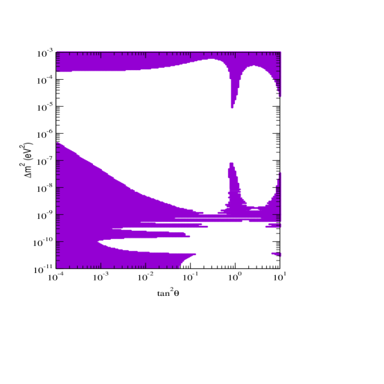
Figure 4.1: The quasi-energy independent regions in $\Delta m^{2}-\tan^{2}\theta$ parameter space where the solar neutrino survival probability agrees with eq. (4.2) to within 10% over the range of Ga to SK energies.

One can easily check that averaging over the SK energy bins of 0.5 MeV has the effect of washing out the coherent term contribution for $\Delta m^{2}>2\times 10^{-9}\ {\rm eV}^{2}$. But including this term enables us to trace the contour down to its lower limit. It was claimed in ref. [18] that the lower strip disappears when one includes the coherent term contribution. This may be due to the fact that their predicted rate in the SK energy range was not integrated over the corresponding bin widths of 0.5 MeV.

To get further insight into the oscillation phenomenon in the maximal mixing region we have plotted in fig. 4.2 the predicted survival rates at maximal mixing against $\Delta m^{2}$ for the Ga, Cl, SK and SNO experiments. In each case the rate has been averaged over the corresponding energy spectrum. This is similar to the fig. 7 of Gonzalez-Garcia, Pena-Garay, Nir and Smirnov [10]. As in [10] the predictions have been shown relative to the central value of the various neutrino fluxes of BPB00 along with those differing by $\pm 1\sigma$ from the central value, e.g. for the ${}^{8}{B}~{}$flux $X_{B}=1\pm 0.2$. We have found that these curves are in good agreement with the corresponding ones of [10]. The two regions of $<10\%$ energy dependence for maximal mixing are indicated by vertical lines. One can easily check that in these regions the central curves lie within 10% of the energy independent prediction $R=0.5$ (note that the SK rate apparently looks higher due to the neutral current contribution). One can clearly see the energy dependence due to the violent oscillations in the VO region (on the left) and the Earth regeneration peak in the LOW region (in the middle), particularly for the Ga experiment. It should be noted that the gap between the two energy independent regions due to the Earth regeneration effect in fig. 4.1 is a little narrower than here. This is due to a cancellation between the positive contribution from the Earth regeneration effect and the negative contribution from the solar matter effect at $\tan^{2}\theta<1$. It ensures that the resulting survival rate agrees with the energy independent solution (4.2) over a somewhat larger range of $\Delta m^{2}$ slightly below the maximal mixing angle.

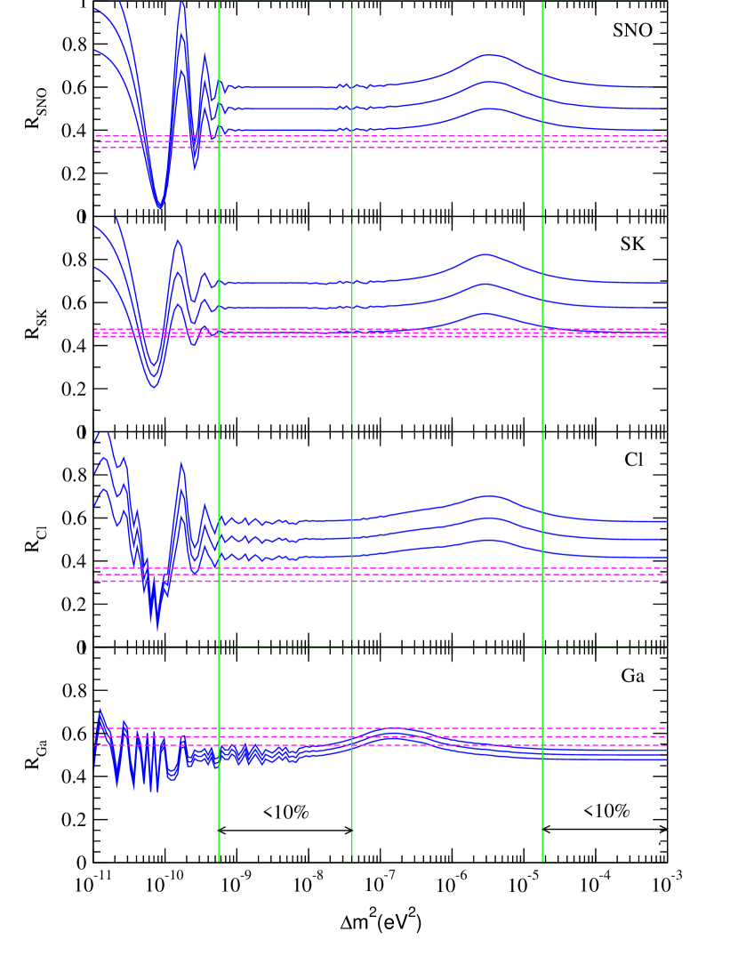
Figure 4.2: The predicted survival rates at maximal mixing against $\Delta m^{2}$ for Cl, Ga, SK and SNO experiments (See text for details.)

The observed rates from the Ga, Cl, SK and SNO experiments are shown in fig. 4.2 as horizontal lines along with their $1\sigma$ errors. With 20% downward renormalisation of the ${}^{8}{B}~{}$neutrino flux $(X_{B}=0.8)$ the energy independent prediction is seen to agree with the SK rate and also approximately with SNO. It is higher than the Cl rate by about $2\sigma$. The agreement with the Ga rate can be improved by going to a little smaller $\theta$ and compensating the resulting deviation from the other rates by a somewhat smaller $X_{B}$ as in Table 4.1. Nonetheless the maximal mixing solution for $X_{B}=0.8$, shown here, is in reasonable agreement with the observed rates over the energy independent regions. The Earth regeneration effect can be seen to improve the agreement with the Ga experiment for the LOW solution.

4.3 The SMA, LMA, LOW and VO Solutions

Tables 4.2 and 4.3 summarise the results of fits to the global rates + spectrum data in terms of the conventional oscillation solutions. Table 4.2 shows solutions to the data with observed and renormalized Cl rate with the neutrino flux of BPB00 $(X_{B}=1)$, while Table 4.3 shows the effects of renormalizing this ${}^{8}{B}~{}$neutrino flux downwards by 25% $(X_{B}=0.75)$. The corresponding 90%, 95%, 99% and 99.73% $(3\sigma)$ contours are shown in fig. 4.3.

	Nature of	$\Delta m^{2}$
	Solution	in eV2	$\tan^{2}\theta$	$\chi^{2}_{min}$	g.o.f
	SMA	$5.28\times 10^{-6}$	$3.75\times 10^{-4}$	51.14	9.22%
Cl	LMA	$4.70\times 10^{-5}$	0.38	33.42	72.18%
Obsvd.	LOW	$1.76\times 10^{-7}$	0.67	39.00	46.99%
	VO	$4.64\times 10^{-10}$	0.57	38.28	50.25%
	SMA	$4.94\times 10^{-6}$	$2.33\times 10^{-4}$	50.94	9.54%
Cl	LMA	$4.70\times 10^{-5}$	0.38	30.59	82.99%
Renorm.	LOW	$1.99\times 10^{-7}$	0.77	34.26	68.57%
	VO	$4.61\times 10^{-10}$	0.59	32.14	77.36%

Table 4.2: The best-fit values of the parameters, the $\chi^{2}_{\min}$ and the g.o.f from a combined analysis of the Cl, Ga, SK and SNO CC rates and the SK day-night spectrum in terms of $\nu_{e}$ oscillation into an active neutrino, including the matter effects. $X_{B}$ is kept fixed at the SSM value (=1.0).

	Nature of	$\Delta m^{2}$
	Solution	in eV2	$\tan^{2}\theta$	$\chi^{2}_{min}$	g.o.f
	SMA	$5.28\times 10^{-6}$	$3.75\times 10^{-4}$	48.39	14.40%
Cl	LMA	$4.65\times 10^{-5}$	0.49	38.90	47.44%
Obsvd.	LOW	$1.74\times 10^{-7}$	0.71	39.91	42.95%
	VO	$4.55\times 10^{-10}$	0.44	37.17	55.36%
	SMA	$8.49\times 10^{-6}$	$1.78\times 10^{-4}$	50.77	9.82%
Cl	LMA	$4.64\times 10^{-5}$	0.51	34.48	67.61%
enorm.	LOW	$2.09\times 10^{-7}$	0.81	33.47	71.97%
	VO	$4.59\times 10^{-10}$	0.53	30.63	82.86%

Table 4.3: Best fits to the combined rates and SK day-night spectrum data in terms of $\nu_{e}$ oscillation into active neutrino with a fixed $X_{B}=0.75$.

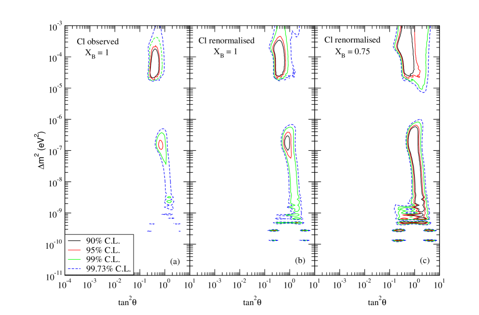
Figure 4.3: The 90%, 95%, 99% and 99.73% C.L. allowed area from the global analysis of the total rates from Cl (observed and 20% renormalized), Ga, SK and SNO (CC) detectors and the 1258 days SK recoil electron spectrum at day and night, assuming conversions to active neutrinos.

As we see from these tables and fig. 4.3 the SMA solution gives rather poor fit in each case, with no allowed contour at $3\sigma$ level. This result agrees with the recent fits of [19] to the global data including SNO. The fit of [20] to these data shows a small allowed region for SMA solution at $3\sigma$ level due to a slightly different method of treating the normalization in the SK spectrum data, as explained there.

The LMA and LOW solutions give good fits to the original data set, which improve further with the upward renormalisation of the Cl rate by $2\sigma$. This is because the monotonic decrease of rate with energy, implied by these solutions, favors the Cl rate to be marginally higher than the SNO and SK rates as mentioned earlier. For the renormalized Cl case, downward renormalisation of the ${}^{8}{B}~{}$neutrino flux by 25% is seen to give a modest increase (decrease) of g.o.f. for the best LOW (LMA) solution. On the other hand the allowed ranges increase in both cases as we see from fig. 4.3b and c. Combined together they imply that the downward renormalisation of the ${}^{8}{B}~{}$neutrino flux modestly favors the LOW solution but makes little difference to the LMA. Its main effect on these two solutions is increasing their allowed ranges in the parameter space. Comparing fig. 4.3c with fig. 4.1 shows that much of these enlarged ranges of validity correspond to effectively energy independent solution. It is interesting to note that the best-fit values of parameters in the LMA region are same for Cl observed and Cl renormalized cases while the $\chi^{2}_{min}$ improves for the latter. This shows that the best-fit already chose a probability at Cl energy, which is a little higher than that at SK/SNO energy. Renormalizing the Cl rate brought that point up to the fitted curve without changing the best-fit parameters.

While the best vacuum solution seems to show remarkably high g.o.f. particularly for renormalized Cl rate and ${}^{8}{B}~{}$neutrino flux, its regions of validity are two miniscule islands just below the lower energy independent strip of fig. 4.3b,c. This solution has also been obtained in the global fits of ref. [19, 20] as well as the SK fit to their rate and spectrum data [22]. The position and size of its range of validity suggest this to be a downward fluctuation of the effectively energy independent quasi vacuum oscillation rather than a genuine VO solution of Just-So type. To get further insight into this solution we have analysed the resulting energy dependence. It shows practically no energy dependence below 5 MeV, but a 15% fall over the $5-12$ MeV range. The latter seems to follow the SK spectral points rather closely amidst large fluctuation. To check the stability of this trend we have repeated the fit to the SK spectral data points, plotted over 8 broad energy bins shown in [22], which show much less fluctuation than the $2\times 19$ points sample. The solution completely disappears from this fit. This confirms that the above VO solution is simply an artifact of the sampling of the SK spectral data.

For completeness we summarise in Table 4.4 the best fits of the above solutions with free ${}^{8}{B}~{}$neutrino flux normalization. The SMA solution favors a very low ${}^{8}{B}~{}$neutrino flux $(X_{B}\simeq 0.5)$, which raises the SK and SNO rates more than the Cl, thus accentuating the nonmonotonic energy dependence of Table 3.2. Still the g.o.f. of the SMA solution is rather marginal. On the other hand the LMA solution favors $X_{B}>1$, which suppresses the SK and SNO rates more than the Cl, resulting in a monotonic decrease of rate with energy. But the corresponding g.o.f. are no better than those of Table 4.2. The results of the LOW and VO fits are similar to those of Table 4.3.

	Nature of		$\Delta m^{2}$
	Solution	$X_{B}$	in eV2	$\tan^{2}\theta$	$\chi^{2}_{min}$	g.o.f
	SMA	0.51	$5.25\times 10^{-6}$	$3.44\times 10^{-4}$	46.83	15.41%
Cl	LMA	1.18	$4.73\times 10^{-5}$	0.33	32.32	72.89%
Obsvd.	LOW	0.88	$1.75\times 10^{-7}$	0.67	38.75	43.57%
	VO	0.70	$4.55\times 10^{-10}$	0.44	37.24	50.44%
	SMA	0.48	$4.66\times 10^{-6}$	$2.32\times 10^{-4}$	46.18	17.01%
Cl	LMA	1.15	$4.71\times 10^{-5}$	0.36	30.32	80.80%
Renorm.	LOW	0.83	$2.03\times 10^{-7}$	0.79	33.18	69.17%
	VO	0.75	$4.63\times 10^{-10}$	0.55	30.56	79.92%

Table 4.4: Best fits to the combined rates and SK day-night spectrum data in terms of $\nu_{e}$ oscillation into active neutrino with $X_{B}$ free.

4.4 Comparisons and Discussions

Let us conclude by briefly discussing whether some of the forthcoming neutrino experiments will be able to discriminate between the energy independent and the MSW solutions. In particular the SNO experiment [23] is expected to provide both the charged current and neutral current scattering rates over roughly the same energy range as SK. Thus the ${}^{8}{B}~{}$neutrino flux can be factored out from their ratio, CC/NC. For oscillations into active neutrino the corresponding double ratio $R_{SNO}^{CC}/R_{SNO}^{NC}$ is predicted to be larger than 0.5 for the energy independent solution and smaller than 0.5 for the LMA and LOW solutions. In the absence of the neutral current data from SNO one can try to make a similar comparison with the ratio of SK elastic and SNO charged current scattering rates,

$$R^{el}_{SK}=X_{B}P_{\nu_{e}\nu_{e}}+r(1-P_{\nu_{e}\nu_{e}})X_{B},\ r=\sigma_{nc}/\sigma_{cc}\simeq 0.17,$$ (4.6)

$$R^{cc}_{SNO}=X_{B}P_{\nu_{e}\nu_{e}},$$ (4.7)

where we have assumed a common survival rate neglecting the small difference between the SK and SNO energy spectra [23]. One can eliminate $P_{\nu_{e}\nu_{e}}$ from the two rates; and the resulting ${}^{8}{B}~{}$neutrino flux can be seen to be in good agreement with the BPB00 estimate [4]. Alternatively one can factor out the flux from the ratio

$$R^{es}_{SK}/R^{cc}_{SNO}=1-r+r/P_{\nu_{e}\nu_{e}}.$$ (4.8)

Table 4.5 shows the best fit values of the above ratio for the LMA, LOW and the energy independent solutions along with the corresponding predictions for $R^{cc}_{SNO}/R^{nc}_{SNO}=P_{\nu_{e}\nu_{e}}$. The predictions of the maximal mixing solution is also shown for comparison. While the LMA and LOW predictions for the $CC/NC$ ratio differ by $\sim 50\%$ they differ by only about $\sim 15\%$ in the case of the $ES/CC$ ratio. The observed ratio $R^{es}_{SK}/R^{cc}_{SNO}$ is seen to favour the LMA over the LOW and energy independent solutions; but even the largest discrepancy is only $\sim 1.5\sigma$. With the expected sample of several thousand $CC$ and $NC$ events from SNO one expects to reduce the $1\sigma$ error for each of these ratios to about 5%. Then one will be able to discriminate between the three solutions meaningfully, particularly with the help of the $CC/NC$ ratio from SNO. On the other hand the LOW solution predicts a large Day-Night asymmetry of $>$ 10% for the ${}^{7}{Be}$ neutrino [10, 11] at the Borexino [24] and the KamLAND [25] experiments. This will be able to distinguish the LOW from the LMA and the energy independent solutions. Lastly it should be noted that the reactor neutrino data at KamLAND is expected to show oscillatory behavior for the LMA solution [26], which will help to distinguish it from the LOW or a generic energy independent solution.

	$\Delta m^{2}$	$\tan^{2}\theta$	$R^{CC}_{SNO}/R^{NC}_{SNO}$	$R^{ES}_{SK}/R^{CC}_{SNO}$	Expt. value of
					$R^{ES}_{SK}/R^{CC}_{SNO}$
LMA	$4.7\times 10^{-5}$	0.38	0.30	1.36
LOW	$1.99\times 10^{-7}$	0.77	0.45	1.19
energy-independent	-	0.47	0.56	1.13	1.33 $\pm$ 0.13
maximal mixing	-	1.0	0.5	1.15

Table 4.5: The values of the ratios $R^{ES}_{SK}/R^{CC}_{SNO}$ and $R^{CC}_{SNO}/R^{NC}_{SNO}$ at the best-fit values for the LMA, LOW and energy independent solutions for the renormalized Cl and $X_{B}=1.0$ case. Also shown are the predictions for the maximal mixing ($P_{ee}=0.5$) solution and the experimental value of $R^{ES}_{SK}/R^{CC}_{SNO}$.

In summary the recent SK data on day/night spectrum is in potential conflict with the apparent energy dependence in the suppression rates observed in Ga, Cl, SK and SNO experiments. Including matter effects one can get acceptable oscillation solutions to both rates and spectrum data only over limited regions of mass and mixing parameters. However an upward renormalisation of the Cl rate by 20% $(2\sigma)$ results in substantial improvement of the quality of fit. Moreover a downward renormalisation of the ${}^{8}{B}~{}$neutrino flux by 25% $(1.5\sigma)$ as suggested by the helioseismic model enlarges the allowed region of the parameter space substantially. Over most of this enlarged region the energy dependence resulting from the matter effects is too weak to be discernible at the present level of experimental accuracy. Hence with these renormalisations of the Cl rate and the ${}^{8}{B}~{}$neutrino flux the data can be described very well by an energy independent solution.

Chapter 5 A Three Generation Oscillation Analysis of the Super-Kamiokande Atmospheric Neutrino Data Beyond One Mass Scale Dominance Approximation

In chapter 3 we have made detailed analysis of the solar and atmospheric neutrino data and presented our results in the two generation framework. In real world there are three active flavors of neutrinos [1]. If one wants to do an analysis of the SK atmospheric neutrino data [2] in a three-generation framework, then there are two possibilities. The most popular three-generation picture in the context of the SK data is the one where one of the mass squared differences is in the solar neutrino range and the other is suitable for atmospheric neutrino oscillations [3, 4, 5, 6, 7, 8]. In such a scheme one mass scale dominance (OMSD) applies for atmospheric neutrinos and the relevant probabilities are functions of two of the mixing angles and one mass squared difference. This picture however cannot explain the LSND results [9]. In this chapter we perform a three flavor $\chi^{2}$-analysis of the SK atmospheric neutrino data assuming a mass pattern with $\Delta_{12}\simeq\Delta_{13}$ fixed in the eV² range (henceforth $\Delta m_{ij}^{2}\equiv\Delta_{ij}$) and allowing the other mass scale to vary arbitrarily. We also incorporate the CHOOZ reactor results [10] into the analysis. Apart from being suitable to explain the SK atmospheric neutrino data this spectrum is also interesting for the laboratory based neutrino oscillation experiments as the higher mass scale is explorable in the short base line experiments, whereas the lower mass scale can be probed in the long base line experiments. In this scheme to a good approximation, neutrino oscillation in the short-base line accelerators and reactors will be governed by one (the higher) mass scale [11, 12] – and only two of the mixing angles appear in the expressions for the oscillation probabilities. For the atmospheric and the long baseline experiments the characteristic energy and length scales are such that in general both mass differences are of relevance and the probabilities involve all the three mixing angles. However the higher mass scale gives rise to $\Delta{m}^{2}$ independent average oscillations and it does not enter the $\chi^{2}$ fit directly. We determine the best-fit values of $\Delta_{23}$ and the three mixing angles by performing a $\chi^{2}$ analysis of the

• SK atmospheric neutrino data

• SK atmospheric and CHOOZ data

We do a bin by bin analysis of the data taking into account the errors and their correlations and use the $\chi^{2}$ function described in eq. (3.62) of chapter 3. Finally we compare the allowed values of the mixing angles as obtained from the above analysis with those allowed by the other accelerator and reactor neutrino oscillation data including LSND and KARMEN2.

The mass scheme of this paper was first considered in [13, 14] after the declaration of the LSND result. These papers performed a combined three generation analysis of accelerator and reactor results as well as the Kamiokande atmospheric neutrino data. Three-generation picture with the higher mass difference in the eV² range and the lower mass difference in the atmospheric range has also been considered in [15, 16] (pre-SK) and [17, 18, 19, 20] (post-SK). These papers attempted to explain both solar and atmospheric neutrino anomalies mainly by maximal $\nu_{\mu}\leftrightarrow\nu_{e}$ oscillations driven by $\Delta_{ATM}\sim 10^{-3}$ eV². Although it was claimed in [17, 18] that this scenario can provide a good fit to all the available data on neutrino oscillations, it was shown in [19] and also later in [20] that this scenario cannot reproduce the zenith angle dependence of the SK atmospheric neutrino data.

In this chapter our aim is to determine the allowed oscillation parameter ranges consistent with SK atmospheric, CHOOZ, LSND and other accelerator and reactor experiments. The solar neutrino problem can be explained by invoking a sterile neutrino. We discuss in the conclusions how the solar neutrino flux suppression can be explained in our scenario.

The plan of the chapter is as follows. In section 5.1.1 we present the formalism for three-generation oscillation analysis in vacuum. We calculate the required probabilities including the earth matter effects in section 5.1.2. We use this expression of the probability for the actual calculation of the number of events. In section 5.2 we present the three-generation $\chi^{2}$ analysis of only SK atmospheric neutrino data using the computer code described in detail in chapter 3. In section 5.3 we present the combined $\chi^{2}$ analysis of SK and CHOOZ data. In section 5.4 we compare the allowed values of mixing angles from the above analyses with those allowed by the other accelerator and reactor data including the latest results from LSND and KARMEN2. In section 5.5 we discuss the implications of our results for the future long baseline experiments and end in section 5.6 with some discussions and conclusions.

5.1 Three-Flavor Analysis

5.1.1 The Vacuum Oscillation Probabilities

The general expression for the probability that an initial $\nu_{\alpha}$ of energy $E$ gets converted to a $\nu_{\beta}$ after traveling a distance $L$ in vacuum is given by eq. (2.6) in chapter 2. The actual forms of the various survival and transition probabilities depend on the neutrino mass spectrum assumed and the choice of the mixing matrix $U$ relating the flavor eigenstates to the mass eigenstates. We choose the flavor states $\alpha=$ 1,2, and 3 to correspond to e, $\mu$ and $\tau$ respectively. The most suitable parameterization of $U$ for the mass spectrum chosen by us is $U=R_{13}R_{12}R_{23}$ where $R_{ij}$ denotes the rotation matrix in the $ij$-plane. This yields:

$$U={\pmatrix{c_{12}c_{13}&s_{12}c_{13}c_{23}-s_{13}s_{23}&c_{13}s_{12}s_{23}+s_{13}c_{23}\cr-s_{12}&c_{12}c_{23}&c_{12}s_{23}\cr-s_{13}c_{12}&-s_{13}s_{12}c_{23}-c_{13}s_{23}&-s_{12}s_{13}s_{23}+c_{13}c_{23}\cr}}$$ (5.1)

where $c_{ij}=\cos{{\theta}_{ij}}$ and $s_{ij}=\sin{{\theta}_{ij}}$ here and everywhere else in this chapter. We have assumed CP-invariance so that $U$ is real. The above choice of $U$ has the advantage that ${\theta}_{23}$ does not appear in the expressions for the probabilities for the laboratory experiments [14].

The probabilities relevant for atmospheric neutrinos are

$$P_{\nu_{e}\nu_{e}} = 1-2c_{13}^{2}c_{12}^{2}+2c_{13}^{4}c_{12}^{4}-4(c_{13}s_{12}c_{23}-s_{13}s_{23})^{2}(c_{13}s_{12}s_{23}+s_{13}c_{23})^{2}~{}\rm S_{23}$$ (5.2)

$$P_{\nu_{\mu}\nu_{e}} = 2c_{13}^{2}c_{12}^{2}s_{12}^{2}-4c_{12}^{2}c_{23}s_{23}(c_{13}s_{12}c_{23}-s_{13}s_{23})(c_{13}s_{12}s_{23}+s_{13}c_{23})~{}\rm S_{23}$$ (5.3)

$$P_{\nu_{\mu}\nu_{\mu}} = 1-2c_{12}^{2}s_{12}^{2}-4c_{12}^{4}c_{23}^{2}s_{23}^{2}~{}\rm S_{23}$$ (5.4)

where $\rm S_{23}=\sin^{2}(\pi L/\lambda_{23})$, where $\lambda_{ij}$ is given by eq. (2.7). Apart from the most general three generation regime, the following limits are of interest, as we will see later in the context of the SK data:

1. The two-generation limits
   Because of the presence of more parameters as compared to the one mass scale dominance picture there are twelve possible two-generation limits [21] with the oscillations driven by either $\Delta_{LSND}$ or $\Delta_{ATM}$. Below we list these limits specifying the mass scales that drive the oscillations:

   • $s_{12}\rightarrow 0,s_{13}\rightarrow 0~{}~{}(\nu_{\mu}-\nu_{\tau},~{}~{}\Delta_{ATM}$), $~{}~{}~{}s_{12}\rightarrow 0,s_{13}\rightarrow 1~{}~{}(\nu_{\mu}-\nu_{e},~{}~{}\Delta_{ATM}$)
     $s_{12}\rightarrow 1,s_{13}\rightarrow 0~{}~{}(\nu_{e}-\nu_{\tau},~{}~{}\Delta_{ATM}$), $~{}~{}~{}s_{12}\rightarrow 1,s_{13}\rightarrow 1~{}~{}(\nu_{e}-\nu_{\tau},~{}~{}\Delta_{ATM}$)

   • $s_{13}\rightarrow 0,s_{23}\rightarrow 0~{}~{}(\nu_{\mu}-\nu_{e},~{}~{}\Delta_{LSND}$), $~{}~{}~{}s_{13}\rightarrow 1,s_{23}\rightarrow 0~{}~{}(\nu_{\mu}-\nu_{\tau},~{}~{}\Delta_{LSND}$)
     $s_{13}\rightarrow 0,s_{23}\rightarrow 1~{}~{}(\nu_{\mu}-\nu_{e},~{}~{}\Delta_{LSND}$), $~{}~{}~{}s_{13}\rightarrow 1,s_{23}\rightarrow 1~{}~{}(\nu_{\mu}-\nu_{\tau},~{}~{}\Delta_{LSND}$)

   • $s_{12}\rightarrow 0,s_{23}\rightarrow 0~{}~{}(\nu_{e}-\nu_{\tau},~{}~{}\Delta_{LSND}$), $~{}~{}s_{12}\rightarrow 1,s_{23}\rightarrow 0~{}~{}(\nu_{e}-\nu_{\tau},~{}~{}\Delta_{ATM}$)
     $s_{12}\rightarrow 0,s_{23}\rightarrow 1~{}~{}(\nu_{e}-\nu_{\tau},~{}~{}\Delta_{LSND}$), $~{}~{}s_{12}\rightarrow 1,s_{23}\rightarrow 1~{}~{}(\nu_{e}-\nu_{\tau},~{}~{}\Delta_{ATM}$)

2. $s_{12}^{2}$ = 0.0
   In this limit the relevant probabilities become

   $$P_{{\nu_{e}}{\nu_{e}}} = 1-2c_{13}^{2}s_{13}^{2}+4s_{13}^{2}c_{23}^{2}s_{23}^{2}S_{23}$$ (5.5)

   $$P_{{\nu_{e}}{\nu_{\mu}}} = 4s_{13}^{2}s_{23}^{2}c_{23}^{2}S_{23}$$ (5.6)

   $$P_{{\nu_{\mu}}{\nu_{\mu}}} = 1-4c_{23}^{2}s_{23}^{2}S_{23}$$ (5.7)

   Thus $P_{{\nu_{\mu}}{\nu_{\mu}}}$ is the same as the two generation limit, $P_{{\nu_{\mu}}{\nu_{e}}}$ is governed by two of the mixing angles and one mass scale and $P_{{\nu_{e}}{\nu_{e}}}$ is governed by two mixing angles and both mass scales.

3. $s_{13}^{2}$ = 0.0
   For this case the probabilities take the form

   $$P_{{\nu_{e}}{\nu_{e}}} = 1-2c_{12}^{2}s_{12}^{2}-4s_{12}^{4}c_{23}^{2}s_{23}^{2}S_{23}$$ (5.8)

   $$P_{{\nu_{e}}{\nu_{\mu}}} = 2c_{12}^{2}s_{12}^{2}-4c_{12}^{2}s_{12}^{2}c_{23}^{2}s_{23}^{2}S_{23}$$ (5.9)

   $$P_{{\nu_{\mu}}{\nu_{\mu}}} = 1-2c_{12}^{2}s_{12}^{2}-4c_{12}^{4}c_{23}^{2}s_{23}^{2}S_{23}$$ (5.10)

   In this case the probabilities are governed by two mass scales and two mixing angles.

We note that for cases (2) and (3) the probabilities are symmetric under the transformation $\theta_{23}\rightarrow\pi/2-\theta_{23}$. The probabilities for these cases are functions of at most two mixing angles as in the OMSD case [3] but they are governed by both mass scales making these limits different from the OMSD limit.

5.1.2 Earth Matter Effects

Since on their way to the detector the upward going neutrinos pass through the earth, it is important in general to include the matter effect in the atmospheric neutrino analysis. The matter contribution to the effective squared mass of the electron neutrinos:

$$A=2{\sqrt{2}}~{}G_{F}~{}E~{}n_{e}$$ (5.11)

where $E$ is the neutrino energy and $n_{e}$ is the ambient electron density. Assuming a typical density of 5 gm/cc and $E$ = 10 GeV, the matter potential $A\simeq 3.65\times 10^{-3}$ eV² and since this is of the same order as $\Delta_{23}$ in our case, matter effects should be studied carefully.

The mass matrix in the flavor basis in presence of matter is given by

$$M_{F}^{2}=U~{}M^{2}~{}U^{\dagger}~{}+~{}M_{A}$$ (5.12)

where $M^{2}$ is the mass matrix in the mass eigenbasis, $U$ is the mixing matrix and

$$M_{A}={\pmatrix{A&0&0\cr 0&0&0\cr 0&0&0\cr}}$$ (5.13)

Since $\Delta_{12}\sim\Delta_{13}\gg\Delta_{23}\sim A$, one can solve the eigenvalue problem using the degenerate perturbation theory, where the $\Delta_{23}$ and $A$ terms are treated as a perturbation to the dominant $\Delta_{12}$ and $\Delta_{13}$ dependent terms. The mixing angle in matter is then given by

$$\tan 2\theta_{23}^{M}=\frac{\Delta_{23}\sin 2\theta_{23}-As_{12}\sin 2\theta_{13}}{\Delta_{23}\cos 2\theta_{23}-A(s_{13}^{2}-c_{13}^{2}s_{12}^{2})}$$ (5.14)

while the mass squared difference in matter turns out to be

$$\Delta_{23}^{M}={\left[(\Delta_{23}\cos 2\theta_{23}-A(s_{13}^{2}-c_{13}^{2}s_{12}^{2}))^{2}+(\Delta_{23}\sin 2\theta_{23}-As_{12}\sin 2\theta_{13})^{2}\right]}^{1/2}$$ (5.15)

The mixing angles $\theta_{12}$ and $\theta_{13}$ as well as the larger mass squared difference $\Delta_{12}$ remain unaltered in matter. From eq. (5.14) and (5.15) we note the following

• In the limit of both $s_{12}\rightarrow 0$ and $s_{13}$ $\rightarrow 0$, the matter effect vanishes and we recover the two-generation $\nu_{\mu}-\nu_{\tau}$ limit.

• The resonance condition now becomes $\Delta_{23}\cos 2\theta_{23}=A(s_{13}^{2}-c_{13}^{2}s_{12}^{2})$. So that for $\Delta_{23}>0$, one can have resonance for both neutrinos – if $s_{13}^{2}>c_{13}^{2}s_{12}^{2}$ – as well as for antineutrinos – if $s_{13}^{2}<c_{13}^{2}s_{12}^{2}$. This is different from the OMSD picture where for $\Delta m^{2}>0$ only neutrinos can resonate.

• In the limit of $s_{12}\rightarrow 0$

  $$\tan 2\theta_{23}^{M}=\frac{\Delta_{23}\sin 2\theta_{23}}{\Delta_{23}\cos 2\theta_{23}-As_{13}^{2}}$$ (5.16)

  Here one gets resonance for neutrinos only (if $\Delta_{23}>0$).

• In the limit $s_{13}\rightarrow 0$

  $$\tan 2\theta_{23}^{M}=\frac{\Delta_{23}\sin 2\theta_{23}}{\Delta_{23}\cos 2\theta_{23}+As_{12}^{2}}$$ (5.17)

  For this case for $\Delta_{23}>0$, there is no resonance for neutrinos but antineutrinos can resonate.

• In the limit where $\Delta_{23}\rightarrow 0$

  $$\tan 2\theta_{23}^{M}=\frac{s_{12}\sin 2\theta_{13}}{s_{13}^{2}-c_{13}^{2}s_{12}^{2}},~{}~{}~{}\Delta_{23}^{M}=A(s_{13}^{2}+c_{13}^{2}s_{12}^{2})$$ (5.18)

  Thus even for small values of $\Delta_{23}<10^{-4}$ the mass squared difference in matter is $\sim A$ and one may still hope to see oscillations for the upward neutrinos due to matter effects. The other point to note is that the mixing angle in matter $\theta_{23}^{M}$ depends only on $\theta_{12}$ and $\theta_{13}$ and is independent of the vacuum mixing angle $\theta_{23}$ and $\Delta_{23}$. Contrast this with the OMSD and the two-generation $\nu_{\mu}-\nu_{e}$ oscillations. For both the two-generation $\nu_{\mu}-\nu_{e}$ as well as the three-generation OMSD case, for $\mbox{$\Delta{m}^{2}$~{}}\rightarrow 0$, the mixing angle in matter $\rightarrow 0$, but for the mass spectrum considered in this paper the $\tan 2\theta_{23}^{M}$ maybe large depending on the values of $s_{12}^{2}$ and $s_{13}^{2}$. Hence we see that the demixing effect which gives the lower bound on allowed values of $\Delta{m}^{2}$ in the two generation $\nu_{\mu}-\nu_{e}$ or the three-generation OMSD case, does not arise here and we hope to get allowed regions even for very low values of $\Delta_{23}$. On the other hand even small values of $\theta_{23}$ in vacuum can get enhanced in matter. This special case where $\Delta_{23}\sim 0$ was considered in an earlier paper [22].

• In the limit of $\mbox{$s_{23}^{2}$}\rightarrow 0$

  $$\tan 2\theta_{23}^{M}=\frac{-As_{12}\sin 2\theta_{13}}{\Delta_{23}-A(s_{13}^{2}-c_{13}^{2}s_{12}^{2})}$$ (5.19)

• While for $\mbox{$s_{23}^{2}$}\rightarrow 1$

  $$\tan 2\theta_{23}^{M}=\frac{-As_{12}\sin 2\theta_{13}}{-\Delta_{23}-A(s_{13}^{2}-c_{13}^{2}s_{12}^{2})}$$ (5.20)

  For the last two cases, corresponding to $\sin^{2}2\theta_{23}\rightarrow 0$, again the mixing angle $\theta_{23}$ in matter is independent of its corresponding value in vacuum and hence for appropriate choices of the other three parameters, $\Delta_{23}$, $s_{12}^{2}$ and $s_{13}^{2}$, one can get large values for $\sin^{2}2\theta_{23}^{M}$ even though the vacuum mixing angle is zero.

The amplitude that an initial $\nu_{\alpha}$ of energy $E$ is detected as $\nu_{\beta}$ after traveling through the earth is

$$A(\nu_{\alpha},t_{0},\nu_{\beta},t)=\sum_{\sigma,\lambda,\rho}\sum_{i,j,k,l} [(U_{\beta l}^{M_{m}}e^{-iE_{l}^{M_{m}}(t-t_{3})}U_{\sigma l}^{M_{m}})(U_{\sigma k}^{M_{m}}e^{-iE_{k}^{M_{c}}(t_{3}-t_{2})}U_{\lambda k}^{M_{c}})\times$$ (5.21)

$$(U_{\lambda j}^{M_{m}}e^{-iE_{j}^{M_{m}}(t_{2}-t_{1})}U_{\rho j}^{M_{m}})(U_{\rho i}e^{-iE_{i}(t_{1}-t_{0})}U_{\alpha i})]$$

where we have considered the earth to be made of two slabs, a mantle and a core with constant densities of 4.5 gm/cc and 11.5 gm/cc respectively and include the non-adiabatic effects at the boundaries. The mixing matrix in the mantle and the core are given by $U^{M_{m}}$ and $U^{M_{c}}$ respectively. $E_{i}^{X}\approx m_{iX}^{2}/2E$, $X$ = core(mantle) and $m_{iX}$ is the mass of the $i^{th}$ neutrino state in the core(mantle). The neutrino is produced at time $t_{0}$, hits the earth mantle at $t_{1}$, hits the core at $t_{2}$, leaves the core at $t_{3}$ and finally hits the detector at time $t$. The Greek indices ($\sigma,\lambda,\rho$) denote the flavor eigenstates while the Latin indices ($i,j,k,l$) give the mass eigenstates. The corresponding expression for the probability is given by

$$P(\nu_{\alpha},t_{0},\nu_{\beta},t)=|A(\nu_{\alpha},t_{0},\nu_{\beta},t)|^{2}$$ (5.22)

For our calculations of the number of events we have used the full expression given by eq.(5.21) and (5.22).

5.2 $\chi^{2}$-analysis of the SK Data

Figure 5.1: The variation of $\Delta\chi^{2}=\chi^{2}-\chi^{2}_{min}$ with one of the parameters keeping the other three unconstrained. The solid (dashed) line corresponds to only SK data when matter effects are included (excluded) while the dotted curve gives the same for SK+CHOOZ. The dashed-dotted line shows the 99% C.L. limit for 4 parameters.

We do a bin by bin $\chi^{2}$ analysis of the 1144 days SK atmospheric neutrino data [23] following the procedure of statistical analysis given in [3, 24]. We minimize the $\chi^{2}$ function defined in chapter 3, eq. (3.62). For contained events there are forty experimental data points. The probabilities for the atmospheric neutrinos are explicit functions of one mass-squared difference and three mixing angles making the number of degrees of freedom (d.o.f) 36. The other mass squared difference gives rise to $\Delta{m}^{2}$ independent average oscillations and hence does not enter the fit as an independent parameter.

For the three-generation scheme considered here the $\chi^{2}_{min}$ and the best-fit values of parameters that we get are

• $\chi^{2}_{min}/d.o.f.=34.65/36$, $\Delta_{23}=0.0027$ eV², $s^{2}_{23}=0.51$,$s_{12}^{2}=0.04$ and $s_{13}^{2}=0.06$

This solution is allowed at 53.28% probability.

The solid(dashed) lines in fig. 5.1 present the variation of the $\Delta\chi^{2}=\chi^{2}-\chi^{2}_{min}$ for the SK data, with respect to one of the parameters keeping the other three unconstrained, when we include(exclude) the matter effect. In fig. 5.1(a) as we go towards smaller values of $\Delta_{23}$ around $10^{-3}$ eV² the effect of matter starts becoming important as the matter term is now comparable to the mass term. If matter effects are not there then for values of $\Delta_{23}$ $\stackrel{{\scriptstyle<}}{{\sim}}10^{-4}$ eV² the $S_{23}$ term in eq. (5.4) is very small and there is no up-down asymmetry resulting in very high values of $\chi^{2}$ as is evident from the dashed curve. If the matter effects are included, then in the limit of very low $\Delta_{23}$ the matter term dominates and $\Delta_{23}^{M}$ is given by eq.(5.18). Since this term $\sim 10^{-3}$ eV² there can be depletion of the neutrinos passing through the earth causing an updown asymmetry. For $\Delta_{23}$ around $10^{-4}$ eV², there is cancellation between the two comparable terms in the numerator of eq. (5.14) and the mixing angle becomes very small and hence the $\chi^{2}$ around these values of $\Delta_{23}$ comes out to be very high.

Fig 5.1(b) illustrates the corresponding variation of $\Delta\chi^{2}$ with $s_{23}^{2}$ while the other three parameters are allowed to vary arbitrarily. For small and large values of $s_{23}^{2}$ the inclusion of matter effect makes a difference. For $s_{23}^{2}$ either very small or large ($\sin^{2}2\theta_{23}\rightarrow 0$) the overall suppression of the $\nu_{\mu}$ flux is less than that required by the data if vacuum oscillation is operative and so it is ruled out. If we include matter effects then in the limit of $s_{23}^{2}=0$ and $s_{23}^{2}=1$ the matter mixing angle is given by eqs. (5.19) and (5.20), which can be large for suitable values of $s_{13}^{2}$ and $s_{12}^{2}$ and hence one gets lower $\chi^{2}$ even for these values of $s_{23}^{2}$.

In figs 5.1(c) and 5.1(d) we show the effect of $s_{12}^{2}$ and $s_{13}^{2}$ respectively on $\Delta\chi^{2}$. From the solid and the dashed lines it is clear that matter effects do not vary much the allowed ranges of $s_{12}^{2}$ and $s_{13}^{2}$.

The dashed-dotted line in the figure shows the 99% C.L. (= 13.28 for 4 parameters) limit. In Table 5.1 we give the allowed ranges of the mixing parameters, inferred from fig. 5.1 at 99% C.L. for the 1144 day SK atmospheric data, with and without matter effects.

	$\Delta_{23}$ in eV2	$s_{23}^{2}$	$s_{12}^{2}$	$s_{13}^{2}$
with	$\!\!1.6\!\!\times\!10^{-4}\!\leq\!\Delta_{23}\!\leq\!7.0\!\!\times\!\!10^{-3}\!\!$	$0.26\leq\mbox{$s_{23}^{2}$}\leq 0.77$	$\mbox{$s_{12}^{2}$}\leq 0.21$	$\mbox{$s_{13}^{2}$}\leq 0.55$
matter effects	$\Delta_{23}\leq 6.5\times 10^{-5}$	$\mbox{$s_{23}^{2}$}\geq 0.85$
without
matter effects	$\!\!5\!\!\times\!\!10^{-4}\!\leq\!\Delta_{23}\!\leq 7.0\!\times\!\!10^{-3}\!\!$	$0.27\leq\mbox{$s_{23}^{2}$}\leq 0.74$	$\mbox{$s_{12}^{2}$}\leq 0.21$	$\mbox{$s_{13}^{2}$}\leq 0.6$

Table 5.1: The allowed ranges of parameters for the 1144 day SK data.

Figure 5.2: (a)The zenith angle distribution of the lepton events with $\Delta_{23}=0.002$ eV² and $s_{23}^{2}$ = 0.5 for various combinations of $s_{12}^{2}$ and $s_{13}^{2}$. $N$ is the number of events as given by eq. (3.58) and $N_{0}$ is the corresponding number with survival probability 1. The panels labelled $SG_{\alpha}$ and $MG_{\alpha}$ ($\alpha$ can be e or $\mu$) give the histograms for the sub-GeV and multi-GeV $\alpha$-events respectively. Also shown are the SK experimental data points with $\pm$ 1$\sigma$ error bars. (b)Same as in (a) for fixed $\mbox{$s_{12}^{2}$}=0.1$ and $\mbox{$s_{13}^{2}$}=0.0$ varying $\Delta_{23}$ and $s_{23}^{2}$.

Figure 5.3: (c)Same as in (a) fixing $\mbox{$s_{12}^{2}$}=0.0$ and $\mbox{$s_{13}^{2}$}=0.1$ for different $\Delta_{23}$ and $s_{23}^{2}$ values. (d)The long-dashed (short-dashed) line gives the zenith angle distribution of the lepton events for the best-fit cases of the two-generation (three-generation) oscillation solutions for SK. The dotted line gives the corresponding distribution for $\Delta_{23}=10^{-5}$ eV², $\mbox{$s_{12}^{2}$}=0.2$, $\mbox{$s_{13}^{2}$}=0.4$ and $\mbox{$s_{23}^{2}$}=1.0$.

5.2.1 Zenith-Angle Distribution

Since the probabilities in our case are in general governed by two mass scales and all three mixing angles it is difficult to understand the allowed regions. To facilitate the qualitative understanding we present in figs. 5.2 and 5.3 the histograms which describe the zenith angle distribution. The event distributions in these histograms are approximately given by,

$$\frac{N_{\mu}}{N_{\mu_{0}}}\approx P_{{\nu_{\mu}}{\nu_{\mu}}}+\frac{N_{e_{0}}}{N_{\mu_{0}}}P_{{\nu_{e}}{\nu_{\mu}}}$$ (5.23)

$$\frac{N_{e}}{N_{e_{0}}}\approx P_{{\nu_{e}}{\nu_{e}}}+\frac{N_{\mu_{0}}}{N_{e_{0}}}P_{{\nu_{\mu}}{\nu_{e}}}$$ (5.24)

where the quantities with suffix 0 indicates the no-oscillation values. For the sub-GeV data $N_{\mu_{0}}/N_{e_{0}}\approx 2$ to a good approximation however for the multi-GeV data this varies in the range 2 (for $\cos\Theta$ =0) to 3 (for $\cos\Theta=\pm$1) [3].

In fig. 5.2(a) we study the effect of varying $s_{12}^{2}$ and $s_{13}^{2}$ for fixed values of $\Delta_{23}$ = 0.002 eV² and $s_{23}^{2}$ = 0.5. From eq. (5.14), (5.15) and from fig. 5.1 we see that for the values of the $\Delta_{23}$ and $s_{23}^{2}$ considered in this figure the matter effects are small and we can understand the histograms from the vacuum oscillation probabilities. The thick solid line shows the event distribution for $s_{12}^{2}=0$ and $s_{13}^{2}=0.1$. As $s_{13}^{2}$ increases from 0, keeping $s_{12}^{2}$ as 0, from eqs. (5.5) and (5.6) $P_{{\nu_{e}}{\nu_{e}}}$ decreases from 1 and $P_{{\nu_{e}}{\nu_{\mu}}}$ increases from zero resulting in a net electron depletion according to eq. (5.24). The long dashed line corresponds to $s_{13}^{2}$ = 0.3 for which the electron depletion is too high as compared to data. The muon events are also affected as $P_{{\nu_{\mu}}{\nu_{e}}}$ increases with increasing $s_{13}^{2}$ even though $P_{{\nu_{\mu}}{\nu_{\mu}}}$ is independent of $s_{13}^{2}$. On the other hand for $s_{13}^{2}$ = 0.0, the effect of increasing $s_{12}^{2}$ is to increase the number of electron events and decrease the number of muon events according to eqs. (5.8), (5.9), (5.10), (5.24) and (5.23). This is shown by the short-dashed and dotted lines in fig. 5.2(a). For $s_{12}^{2}$ = 0.2 the electron excess and muon depletion both becomes too high as compared to the data. For the case when both $s_{12}^{2}$ and $s_{13}^{2}$ are 0.1 the electron depletion caused by increasing $s_{12}^{2}$ and the excess caused by increasing $s_{13}^{2}$ gets balanced and the event distributions are reproduced quite well, shown by the dashed-dotted line.

In fig. 5.2(b) we study the effect of varying $s_{23}^{2}$ and $\Delta_{23}$ in the limit of $s_{12}^{2}=0$ with $s_{13}^{2}$ fixed at 0.1. Although we use the full probabilities including the matter effect, for 0.004 eV² this is not so important and one can understand the histograms from the vacuum oscillation probabilities. For fixed $\Delta_{23}$ as $s_{23}^{2}$ increases, $P_{{\nu_{\mu}}{\nu_{\mu}}}$ decreases, making the muon depletion higher. This is shown in the figure for two representative values of $\Delta_{23}$. The electron events are not affected much by change of $s_{23}^{2}$. The slight increase with $s_{23}^{2}$ is due to increase of both $P_{{\nu_{e}}{\nu_{e}}}$ and $P_{{\nu_{\mu}}{\nu_{e}}}$. To understand the dependence on $\Delta_{23}$ we note that for $\mbox{$s_{23}^{2}$}=0.2$, if one looks at the vacuum oscillation probabilities, $N_{\mu}/N_{\mu 0}\approx 1-0.65S_{23}$. For 0.004 eV² the contribution of $S_{23}$ is more resulting in a lower number of muon events. For the electron events however the behavior with $\Delta_{23}$ is opposite, with $N_{e}/N_{e0}=0.82+0.12S_{23}$. Thus with increasing $\Delta_{23}$ the number of electron events increase. Also note that since the contribution of $S_{23}$ comes with opposite sign the zenith-angle distribution for a fixed $\Delta_{23}$ is opposite for the muon and the electron events.

In fig. 5.3(c) we show the histograms in the limit of $s_{13}^{2}$ = 0.0, keeping $s_{12}^{2}$ as 0.1 and varying $\Delta_{23}$ and $s_{23}^{2}$. As $s_{23}^{2}$ increases all the relevant probabilities decrease and therefore both $N_{\mu}/N_{\mu 0}$ and $N_{e}/N_{e0}$ decrease giving less number of events for both. For this case the $S_{23}$ term comes with the same sign (negative) in both $N_{\mu}/N_{\mu 0}$ and $N_{e}/N_{e0}$. Therefore the depletion is more for higher $\Delta_{23}$ for both muon and electron events.

Finally, the long dashed line in fig. 5.3(d) represent the histograms for the best-fit value for two-generation ${\nu_{\mu}}-{\nu_{\tau}}$ oscillations, for which $P_{{\nu_{e}}{\nu_{e}}}=1$. The short dashed line gives the histograms for the three-generation best-fit values. Both give comparable explanation for the zenith angle distribution of the data. The dotted line gives the event distribution for $\Delta_{23}=10^{-5}$ eV². As discussed earlier even for such low value of $\Delta_{23}$, we find that due to the unique feature of the beyond OMSD neutrino mass spectrum, earth matter effects ensure that both the sub-GeV as well as the multi-GeV upward muon events are very well reproduced, as are the electron events. But since $s_{12}^{2}$ is high, the downward ${\nu_{\mu}}$ are depleted more than the data requires.

5.2.2 Allowed Parameter Region

Figure 5.4: The allowed parameter regions in the $\Delta_{23}-\mbox{$s_{23}^{2}$}$ plane for various fixed values of $s_{12}^{2}$ and $s_{13}^{2}$, shown at the top of each panel. The solid lines corresponds to the 99% C.L. contours from the SK data alone, while the dotted line gives the 99% contour from the combined analysis of the SK+CHOOZ data.

In fig. 5.4 the solid lines give the 99% C.L. allowed area from SK data in the $\Delta_{23}$-$s^{2}_{23}$ plane keeping the values of $s^{2}_{13}$ and $s^{2}_{12}$ fixed in the allowed range from fig. 5.1 and Table 5.1. The first panel represents the two-generation ${\nu_{\mu}}-{\nu_{\tau}}$ oscillation limit modulo the difference in the definition of the C.L. limit as the number of parameters are different. We have seen from the histograms in fig. 5.2(a) that raising $s_{12}^{2}$ results in electron excess and muon depletion. On the other hand increase in $s_{13}^{2}$ causes electron depletion. The above features are reflected in the shrinking and disappearance of the allowed regions in the first row and column. In the panels where both $s_{12}^{2}$ and $s_{13}^{2}$ are nonzero one may get allowed regions only when the electron depletion due to increasing $s_{13}^{2}$ is replenished by the increase in $s_{12}^{2}$.

Figure 5.5: Same as fig. 5.4 but in the bilogarithmic $\tan^{2}\theta_{12}-\tan^{2}\theta_{13}$ plane for fixed values of $\Delta_{23}$ and $s_{23}^{2}$.

In fig. 5.5 we present the 99% C.L. allowed areas in the bilogarithmic $\tan^{2}\theta_{12}-\tan^{2}\theta_{13}$ plane for various fixed values of the parameters $\Delta_{23}$ and $s^{2}_{23}$. We use the $\log(\tan)$ representation which enlarges the allowed regions at the corners and the clarity is enhanced. The four corners in this plot refer to the two-generation limits discussed before. The extreme left corner ($\theta_{12}\rightarrow 0,\theta_{13}\rightarrow 0$) correspond to the two generation $\nu_{\mu}-\nu_{\tau}$ oscillation limit. As we move up increasing $\theta_{13}$, one has $\nu_{e}-\nu_{\mu}$ and $\nu_{e}-\nu_{\tau}$ mixing in addition and for $\mbox{$s_{13}^{2}$}\rightarrow 1$ one goes to the two generation $\nu_{\mu}-\nu_{e}$ oscillation region. For the best-fit values of $\Delta_{23}$ and $s_{23}^{2}$ if we take $s_{12}^{2}$ and $s_{13}^{2}$ to be 0 and $1$ respectively, then the $\chi^{2}_{min}$ is 66.92 which is therefore ruled out. Both the right hand corners in all the panels refer to pure $\nu_{e}-\nu_{\tau}$ oscillations and therefore there are no allowed regions in these zones. For the panels in the first row, $\Delta_{23}=0.006$ eV² and the 2-generation ${\nu_{\mu}}-{\nu_{\tau}}$ oscillation limit is just disallowed. The small area allowed for the middle panel of first row (between the solid lines) is due to the fact that for non-zero $s_{12}^{2}$ and $s_{13}^{2}$ the electron events are better reproduced, while $\mbox{$s_{23}^{2}$}=0.5$ takes care of the muon events. Hence for this case slight mixture of ${\nu_{\mu}}-{\nu_{e}}$ and ${\nu_{e}}-{\nu_{\tau}}$ oscillations is favoured. This feature was also reflected in the fact that in the fig. 5.4, the panel for $\mbox{$s_{12}^{2}$}=0.1$ and $\mbox{$s_{13}^{2}$}=0.3$ has more allowed range for $\Delta_{23}$ than the panel for the 2-generation ${\nu_{\mu}}-{\nu_{\tau}}$ limit. For the panels with $\Delta_{23}=0.002$ eV², both the pure ${\nu_{\mu}}-{\nu_{\tau}}$ limit as well as full three-generation oscillations, give good fit. For the last two rows with $\Delta_{23}=0.0007$ eV² and $0.0004$ eV² the matter effects are important in controlling the shape of the allowed regions. Infact the allowed region that one gets for $0.0004$ eV² and $s_{23}^{2}$ = 0.5 is the hallmark of the matter effect in this particular three-generation scheme. As can be seen from fig. 5.1(a) and Table 5.1, if one does not include the matter effect, then there are no allowed regions below $\Delta_{23}$ = 0.0005 eV² for any arbitrary combination of the other three parameters. Even for the first and the last panels with $\Delta_{23}=0.0007$ eV², one gets allowed areas solely due to matter effects.

Figure 5.6: Same as fig. 5.4 but in the $\mbox{$s_{12}^{2}$}-\mbox{$s_{23}^{2}$}$ plane for fixed values of $s_{13}^{2}$ and $\Delta_{23}$.

In fig. 5.6 the solid lines show the 99% C.L. allowed regions from SK data in the $s^{2}_{23}-s^{2}_{12}$ plane for fixed values of $\Delta_{23}$ and $s^{2}_{13}$. In contrast to the previous figure, here (and in the next figure) we use the $\sin-\sin$ representation because the allowed regions are around $\theta_{23}=\pi/4$ and this region gets compressed in the $\log(\tan)-\log(\tan)$ representation. For explaining the various allowed regions we separate the figures in two sets

$\bullet$ For $s^{2}_{13}$ = 0.0, the four corners of the panels represent the no-oscillation limits inconsistent with the data. Also as discussed in the earlier sections for $s_{23}^{2}$ = 0.0 or 1.0 one goes to the limit of pure $\nu_{\mu}-\nu_{e}$ conversions driven by $\Delta_{LSND}$, which is not consistent with data. One obtains allowed regions only when $s^{2}_{23}$ is close to 0.5 with $s_{12}^{2}$ small, so that ${\nu_{\mu}}-{\nu_{\tau}}$ conversions are dominant. The allowed range of $s_{12}^{2}$ is controlled mainly by the electron excess as has been discussed before while the allowed range of $s_{23}^{2}$ is determined mostly by the muon depletion.

$\bullet$ For $s_{13}^{2}\neq 0$, the four corners represent the two-generation $\nu_{e}-\nu_{\tau}$ oscillation limit and hence these corners are not allowed. For $s_{23}^{2}=0.0$ or 1.0 and $s_{12}^{2}\neq$ 0 or 1 one has $\Delta_{LSND}$ driven ${\nu_{\mu}}-{\nu_{e}}$ and ${\nu_{\mu}}-{\nu_{\tau}}$ conversion and $\Delta_{ATM}$ driven $\nu_{e}-\nu_{\tau}$ conversions. This scenario is not allowed as it gives excess of electron events and also fails to reproduce the correct zenith angle dependence. For a fixed $\Delta_{23}$ as $s_{13}^{2}$ increases the electron depletion increases which can be balanced by increasing $s_{12}^{2}$ which increases the number of electron events. Hence for a fixed $\Delta_{23}$ the allowed regions shift towards higher $s_{12}^{2}$ values.

As in fig. 5.5 the allowed area in the middle panel of the last row is due to the inclusion of the matter effect.

Figure 5.7: Same as fig. 5.4 but in the $\mbox{$s_{13}^{2}$}-\mbox{$s_{23}^{2}$}$ plane for various fixed values of $s_{12}^{2}$ and $\Delta_{23}$.

In fig. 5.7 the solid contours refer to the 99% C.L. allowed areas from SK atmospheric neutrino data in the $s^{2}_{13}-s^{2}_{23}$ plane for various values of $\Delta_{23}$ and $s^{2}_{12}$.

$\bullet$ For $s_{12}^{2}$ = 0.0 the corners represent no oscillation limits. In the limit $\mbox{$s_{23}^{2}$}\rightarrow 0$ or 1, one gets ${\nu_{e}}-{\nu_{\tau}}$ oscillation driven by $\Delta_{LSND}$ which is also not allowed. For $s_{13}^{2}$ = 0.0 and $\mbox{$s_{23}^{2}$}\sim 0.5$ one has maximal two-flavour ${\nu_{\mu}}-{\nu_{\tau}}$ oscillation limit which is therefore allowed (not allowed for $\Delta_{23}=0.006$ eV² as discussed before). As $s_{13}^{2}$ increases the electron depletion becomes higher and that restricts higher $s_{13}^{2}$ values.

$\bullet$ For $s_{12}^{2}\neq 0$, the four corners represent two-generation limits driven by $\Delta_{LSND}$. This is the regime of average oscillations and cannot explain the zenith angle dependence of the data. For a fixed $\Delta_{23}$ the allowed region first expands and then shrinks in size and also shifts towards higher $s_{13}^{2}$ values as $s_{12}^{2}$ increases just as in fig. 5.6.

Matter effect is important for the last two rows and the increase in the allowed areas for the last two panels of $\Delta_{23}=0.0004$ eV² are typical signatures of matter effect.

Figure 5.8: The allowed parameter space in the $\Delta_{23}-\mbox{$s_{23}^{2}$}$ plane with $\Delta_{23}$ in the range $10^{-5}-10^{-4}$ eV² and with fixed values of $\mbox{$s_{12}^{2}$}=0.185$ and $\mbox{$s_{13}^{2}$}=0.372$.

In fig. 5.8 we present the allowed range in the $\Delta_{23}-\mbox{$s_{23}^{2}$}$ plane with $\Delta_{23}$ in the $10^{-5}-10^{-4}$ eV² range and $s_{12}^{2}$, $s_{13}^{2}$ fixed at 0.185 and 0.372 respectively. We get allowed regions in this range of small $\Delta_{23}$ and small mixing due to matter effects – a feature unique to the mass spectrum considered in this chapter.

5.3 $\chi^{2}$ analysis of the SK + CHOOZ Data

The CHOOZ experiment can probe upto $10^{-3}$ eV² and hence it can be important to cross-check the atmospheric neutrino results. In particular a two-generation analysis shows that CHOOZ data disfavours the $\nu_{\mu}-\nu_{e}$ solution to the atmospheric neutrino problem. The general expression for the survival probability of the electron neutrino in presence of three flavours is

$$P_{\nu_{e}\nu_{e}}=1-4U_{e1}^{2}(1-U_{e1}^{2}){\sin^{2}}({\pi L/\lambda_{12})}-4U_{e2}^{2}U_{e3}^{2}{\sin^{2}}({\pi L/\lambda_{23}})$$ (5.25)

This is the most general expression without the one mass scale dominance approximation. We now minimize the $\chi^{2}$ defined as

$$\chi^{2}=\chi^{2}_{ATM}+\chi^{2}_{CHOOZ}$$ (5.26)

where $\chi^{2}_{ATM}$ is calculated as before using eq. (3.62) and we define $\chi^{2}{{}_{CHOOZ}}$ as [25]

$$\chi^{2}_{CHOOZ}=\sum_{j=1,15}(\frac{x_{j}-y_{j}}{\Delta x_{j}})^{2}$$ (5.27)

where $x_{j}$ are the experimental values, $y_{j}$ are the corresponding theoretical predictions and the sum is over 15 energy bins of data of the CHOOZ experiment [10]. For the CHOOZ experiment the $\sin^{2}(\pi L/\lambda_{12})$ term does not always average out to 0.5 (for SK this term always averages to 0.5) and one has to do the energy integration properly. For our analysis we keep the $\Delta_{12}$ fixed at 0.5 eV² and do a four parameter fit as in SK. The $\chi^{2}_{min}$ and the best-fit values of parameters that we get are

• $\chi^{2}_{min}/d.o.f.=42.22/51$, $\Delta_{23}$ = 0.0023 eV², $s^{2}_{23}=0.5$, $s_{12}^{2}=0.0022$ and $s_{13}^{2}=0.0$.

Thus the best-fit values shift towards the two-generation limit when we include the CHOOZ result. This provides a very good fit to the data being allowed at 80.45% probability.

Figure 5.9: Same as fig. 5.4 but for smaller values of $s_{12}^{2}$ and $s_{13}^{2}$, chosen from the range determined by the SK+CHOOZ dashed line in fig. 5.1.

The dotted lines in fig. 5.1 give the combined SK+CHOOZ $\Delta\chi^{2}(=\chi^{2}-\chi^{2}_{min})$ given by eq. (5.26), as a function of one of the parameters, keeping the other three unconstrained. We find that the CHOOZ data severely restricts the allowed ranges for the parameters $s_{12}^{2}$ and $s_{13}^{2}$ to values $\stackrel{{\scriptstyle<}}{{\sim}}0.047$, while $\Delta_{23}$ and $s_{23}^{2}$ are left almost unaffected. Since CHOOZ is consistent with no oscillation one requires $P_{{\nu_{e}}{\nu_{e}}}$ close to 1. So the second and the third terms in eq. (5.25) should separately be very small. The second term implies $U_{e1}^{2}$ to be close to either 0 or 1. $U_{e1}^{2}$ close to zero implies either $s_{12}^{2}$ or $s_{13}^{2}$ close to 1 which is not consistent with SK. Therefore $U_{e1}^{2}$ is close to 1. Then from unitarity both $U_{e2}^{2}$ and $U_{e3}^{2}$ are close to 0 and so the third term goes to zero irrespective of the value of $\Delta_{23}$ and $s_{23}^{2}$. Hence contrary to expectations, CHOOZ puts almost no restriction on the allowed values of $s_{23}^{2}$ and $\Delta_{23}$, although $\Delta_{23}\sim 10^{-3}$ eV² – in the regime in which CHOOZ is sensitive. On the other hand it puts severe constraints on the allowed values of $s_{12}^{2}$ and $s_{13}^{2}$ in order to suppress the average oscillations driven by $\Delta_{12}$. Because of such low values of $s_{12}^{2}$ and $s_{13}^{2}$ the matter effects for the atmospheric neutrinos are not important and the additional allowed area with low $\Delta_{23}$ and high $s_{23}^{2}$ obtained in the SK analysis due to matter effects are no longer allowed. The 99% C.L. regions allowed by a combined analysis of SK and CHOOZ data is shown by the dotted lines in figs. 5.4-5.7. It is seen that most of the regions allowed by the three-flavour analysis of the SK data is ruled out when we include the CHOOZ result. None of the allowed regions shown in fig. 5.4 are allowed excepting the two-generation ${\nu_{\mu}}-{\nu_{\tau}}$ oscillation limit because CHOOZ does not allow such high values of either $s_{13}^{2}$ or $s_{12}^{2}$. Hence we present again in fig. 5.9 the allowed regions in the $\Delta_{23}-\mbox{$s_{23}^{2}$}$ plane for various fixed values of $s_{12}^{2}$ and $s_{13}^{2}$, determined from the dotted lines in fig. 5.1. The solid lines in fig. 5.9 give the 99% C.L. area allowed by the SK data while the dotted lines give the corresponding allowed region from the combined analysis of SK+CHOOZ. We find that for the combined analysis we get allowed regions in this plane only for much smaller values of $s_{12}^{2}$ and $s_{13}^{2}$, which ensures that the electron events are neither less nor more than expectations.

5.4 Combined Allowed Area from Short Baseline Accelerator and Reactor Experiments

As mentioned earlier the higher mass scale of this scenario can be explored in the accelerator based neutrino oscillation search experiments. For the mass-pattern considered the most constraining accelerator experiments are LSND [9], CDHSW [26], E531 [27] and KARMEN [28]. Among these only LSND reported positive evidence of oscillation. Other experiments are consistent with no-oscillation hypothesis. Also important in this mass range are the constraints from the reactor experiment Bugey [29]. The relevant probabilities are [14]

• Bugey

  $$P_{\overline{\nu}_{e}\overline{\nu}_{e}}=1-4c_{13}^{2}c_{12}^{2}{\sin^{2}}({\pi L/\lambda_{12}})+4c_{13}^{4}c_{12}^{4}{\sin^{2}}({\pi L/\lambda_{12}})$$ (5.28)

• CDHSW

  $$P_{\overline{\nu}_{\mu}\overline{\nu}_{\mu}}=1-4c_{12}^{2}s_{12}^{2}{\sin^{2}}({\pi L/\lambda_{12}})$$ (5.29)

• LSND and KARMEN

  $$P_{\overline{\nu}_{\mu}\overline{\nu}_{e}}=4c_{12}^{2}s_{12}^{2}c_{13}^{2}{\sin^{2}}({\pi L/\lambda_{12}})$$ (5.30)

• E531

  $$P_{\nu_{\mu}\nu_{\tau}}=4c_{12}^{2}s_{12}^{2}s_{13}^{2}\sin^{2}({\pi L/\lambda_{13}})$$ (5.31)

We note that the probabilities are functions of one of the mass scales and two mixing angles. Thus the one mass scale dominance approximation applies. There are many analyses in the literature of the accelerator and reactor data including LSND under this one mass scale dominance assumption [14, 30]. These analyses showed that when one considers the results from the previous (prior to LSND) accelerator and reactor experiments there are three allowed regions in the $\theta_{12}-\theta_{13}$ plane [14, 30]

• low $\theta_{12}$ - low $\theta_{13}$

• low $\theta_{12}$ - high $\theta_{13}$

• high $\theta_{12}$ - $\theta_{13}$ unconstrained

When the LSND result was combined with these results then only the first and the third zones remained allowed in the mass range $0.5\leq\Delta_{12}\leq 2$ eV². In these earlier analyses of the accelerator and reactor data [14, 30] E776 [31] was more constraining than KARMEN. But with the new data KARMEN2 gives stronger constraint than E776. Also the results from the KARMEN2 experiment now rule out most of the region allowed by the LSND experiment above 1 eV² [28]. The LSND collaboration has also now done a reanalysis of their entire data sample and report their final transition probability in [32]. We have repeated the analysis with the latest LSND and KARMEN results for one representative value of $\Delta_{12}=0.5$ eV² and present the allowed region in fig. 5.10.

Figure 5.10: The area between the dashed lines is the 90% C.L. region allowed by LSND while the light shaded zone gives the 90% C.L. allowed region from the non-observance of neutrino oscillation in the other short baseline accelerator and reactor experiments except KARMEN2. The corresponding area which includes KARMEN2 as well is shown by the region shaded by asterix. The 90% C.L. allowed region from SK+CHOOZ analysis is within the dotted line. The dark shaded area corresponds to the combined allowed region.

The light-shaded area in fig. 5.10 shows the 90% C.L. allowed area in the bilogarithmic $\tan^{2}\theta_{12}-\tan^{2}\theta_{13}$ plane from the observance of no-oscillation in all the other above mentioned accelerator and reactor experiments except KARMEN2. The inclusion of the KARMEN2 results as well gives the 90% C.L. region shown by the area shaded by asterix. The 90% allowed region by the LSND experiment is within the dashed lines. The KARMEN2 data severely restricts the LSND allowed regions. The dotted line shows the 90% C.L. ($\chi^{2}\leq\chi^{2}_{min}+7.78$) region allowed by the combined $\chi^{2}$ analysis of the SK+CHOOZ data keeping $\Delta_{23}$ and $s_{23}^{2}$ at 0.002 eV² and 0.5 respectively. The combined SK atmospheric and the CHOOZ reactor data rule out the third zone (high $\theta_{12}$ with $\theta_{13}$ unconstrained ) allowed from LSND and other accelerator and reactor experiments. Thus if one takes into account constraints from all experiments only a small region in the first zone (small $\theta_{12},\theta_{13}$) remains allowed. This common allowed region is shown as a dark-shaded area in the fig. 5.10. As evident from the expression of the probabilities for the accelerator and reactor experiments the combined allowed area of all the accelerator reactor experiments remains the same irrespective of the value of $\Delta_{23}$ and $s_{23}^{2}$. Even though the combined area in fig. 5.10 shows that in the first zone (small $\theta_{12},\theta_{13}$), SK+CHOOZ data allows more area in the $\theta_{12}-\theta_{13}$ plane for $\Delta_{23}=0.002$ eV² and $\mbox{$s_{23}^{2}$}=0.5$, from fig. 5.5 we see that for some other combinations of $\Delta_{23}$ and $s_{23}^{2}$ one does not find any allowed zones from the SK+CHOOZ analysis, even at 99% C.L.. For those sets of values of $\Delta_{23}$ and $s_{23}^{2}$ the SK+CHOOZ analysis is more restrictive than the LSND and other accelerator reactor data.

5.5 Implications

From our analysis of the SK atmospheric data the explicit form for the $3\times 3$ mixing matrix $U$ at the best-fit values of parameters is

$$U={\pmatrix{0.95&-0.039&0.31\cr-0.2&0.686&0.7\cr-0.24&-0.727&0.644\cr}}$$ (5.32)

From the combined SK+CHOOZ analysis the mixing matrix at the best-fit values of the parameters is

$$U={\pmatrix{0.999&0.033&0.033\cr-0.047&0.706&0.706\cr-0.0&-0.707&0.707\cr}}$$ (5.33)

From the combined allowed area of fig. 5.10 the mixing matrix at $\Delta_{12}$ = 0.5 eV², $\Delta_{23}=0.0028$ eV², $s_{12}^{2}=0.005$, $s_{13}^{2}$ = 0.001 and $s_{23}^{2}$ = 0.5, is

$$U={\pmatrix{0.997&0.028&0.072\cr-0.071&0.705&0.705\cr-0.032&-0.708&0.705\cr}}$$ (5.34)

Thus the allowed scenario corresponds to the one where $\langle\nu_{1}|\nu_{e}\rangle$ is close to 1 while the states $\nu_{2}$ and $\nu_{3}$ are combinations of nearly maximally mixed $\nu_{\mu}$ and $\nu_{\tau}$ .

Figure 5.11: 90% C.L. regions in the $\Delta_{23}-\mbox{$s_{23}^{2}$}$ plane that can be explored by the ${\nu_{\mu}}-{\nu_{\mu}}$ (solid line) and ${\nu_{\mu}}-{\nu_{e}}$ (dashed line) oscillation channels in the K2K experiment. The area inside the dotted line shows the 90% C.L. region allowed by SK+CHOOZ. The curves are presented for fixed values of $s_{12}^{2}$ and $s_{13}^{2}$ with $\Delta_{12}=0.5$ eV².

Long baseline (LBL) experiments can be useful to confirm if the atmospheric neutrino anomaly is indeed due to neutrino oscillations, using well monitored accelerator neutrino beams. Some of the important LBL experiments are K2K (KEK to SK, L $\approx$ 250 km)[33] , MINOS (Fermilab to Soudan, L $\approx$ 730 km ) [35] and the proposed CERN to Gran Sasso experiments (L $\approx$ 730 km) [36]. In this section we explore the sensitivity of the LBL experiment K2K in probing the parameter spaces allowed by the SK+CHOOZ and other accelerator and reactor experiments including LSND. K2K will look for $\nu_{\mu}$ disappearance as well as $\nu_{e}$ appearance. In fig. 5.11 we show the regions in the $\Delta_{23}-\mbox{$s_{23}^{2}$}$ plane that can be probed by K2K using their projected sensitivity from [33]. The top left panel is for the two-generation $\nu_{\mu}-\nu_{\tau}$ limit. The other panels are for different fixed values of $s_{12}^{2}$ and $s_{13}^{2}$ while $\Delta_{12}$ is fixed at 0.5 eV². For LBL experiments the term containing $\Delta_{12}$ averages to 0.5 as in the atmospheric case. The solid lines in the panels show the region that can be probed by K2K using the ${\nu_{\mu}}$ disappearance channel while the dotted lines give the 90% C.L. contours allowed by SK+CHOOZ. One finds that for for $\Delta_{23}\geq 2\times 10^{-3}$ eV², the whole region allowed by SK+CHOOZ can be probed by the $\nu_{\mu}$ disappearance channel in K2K. The dashed lines show the 90% C.L. area that K2K can probe by the ${\nu_{e}}$ appearance mode. As $s_{12}^{2}$ increases the constraint from the $P_{{\nu_{\mu}}{\nu_{e}}}$ channel becomes important as is seen in the top right panel of fig. 5.11. However such high values of $s_{12}^{2}$, although allowed by SK+CHOOZ, is not favoured when one combines LSND and other accelerator and reactor results. For lower $s_{12}^{2}$ values allowed by all the accelerator, reactor and SK atmospheric neutrino experiment the projected sensitivity in the ${\nu_{\mu}}-{\nu_{e}}$ channel of K2K is not enough to probe the allowed regions in the $\Delta_{23}-\mbox{$s_{23}^{2}$}$ plane as is shown by the absence of the dashed curves in the lower panels.

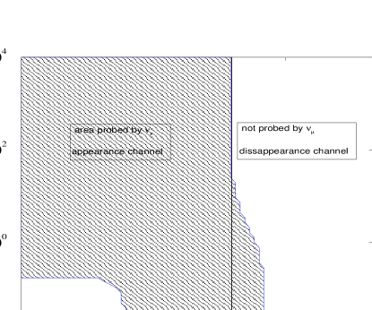
Figure 5.12: Sensitivity of the K2K experiment in the $\tan^{2}\theta_{12}-\tan^{2}\theta_{13}$ plane for $\Delta_{23}=0.002$ eV², $s_{23}^{2}=0.5$ and $\Delta_{12}=0.5$ eV². The area that can be explored by the ${\nu_{\mu}}-{\nu_{\mu}}$ (left of solid line) and ${\nu_{\mu}}-{\nu_{e}}$ (hatched area) channels in K2K at 90% C.L. is shown. The light-shaded area is allowed by SK+CHOOZ and the dark-shaded region is the combined area allowed by all accelerator and reactor data at 90% C.L..

In fig. 5.12 we show the regions in the bilogarithmic $\tan^{2}\theta_{12}-\tan^{2}\theta_{13}$ plane which can be probed by K2K. For drawing these curves we fix $\Delta_{23}=0.002$ eV², $s_{23}^{2}=0.5$ and $\Delta_{12}=0.5$ eV². Shown is the area that can be explored by the ${\nu_{\mu}}-{\nu_{\mu}}$ (left of the solid line) and ${\nu_{\mu}}-{\nu_{e}}$ (hatched area) channels in K2K at 90% C.L.. The light-shaded area is allowed by SK+CHOOZ and the dark shaded area is allowed by the combination of all the accelerator, reactor and SK atmospheric neutrino data at 90% C.L.. It is clear from the figure that even though the sensitivity of the ${\nu_{e}}$ appearance channel is not enough, K2K can still probe the combined allowed region in the $\theta_{12}-\theta_{13}$ plane from ${\nu_{\mu}}$ disappearance.

The projected sensitivities of MINOS and the CERN to ICARUS proposals are lower than K2K and it will be interesting to check if one can probe the regions allowed in this picture better in these experiments. However since in our case the OMSD approximation is not applicable one has to do the energy averaging properly to get the corresponding contours in the three-generation parameters space, and one cannot merely scale the allowed regions from the two-generation plots. For K2K we could use the fig. 5 of [33] to circumvent this problem. However since the analogous information for MINOS and CERN-Gran Sasso proposals is not available to us we cannot check this explicitly.

An important question in this context is whether one can distinguish between the OMSD three generation and this mass scheme. In both pictures the SK atmospheric neutrino data can be explained by the dominant $\nu_{\mu}-\nu_{\tau}$ oscillations mixed with little amount of $\nu_{e}-\nu_{\mu}(\nu_{\tau})$ transition. However the mixing matrix $U$ is different. A distinction can be done if one can measure the mixing angles very accurately.

What is the prospect in LBL experiments to distinguish between these pictures? We give below a very preliminary and qualitative discussion on this. If we take $s_{12}^{2}$ = 0.02, $s_{13}^{2}$ = 0.02 and $s_{23}^{2}$ = 0.5, $P_{{\nu_{\mu}}{\nu_{e}}}$ would be (0.038 + 0.0004 $\langle S_{23}\rangle$). As the second term is negligible one has average oscillations. This is different from the OMSD limit where $P_{{\nu_{\mu}}{\nu_{e}}}=4U_{\mu 3}^{2}U_{e3}^{2}S_{23}$ is energy dependent. If one combines the other accelerator and reactor experiments including LSND then the allowed values of of $s_{12}^{2}$ and $s_{13}^{2}$ are even less and choosing $s_{12}^{2}$ = 0.005, $s_{13}^{2}$ = 0.001 and $s_{23}^{2}$ = 0.5 we get $P_{{\nu_{e}}{\nu_{\mu}}}=0.01-0.004\langle S_{23}\rangle$. Here also the term involving $\langle S_{23}\rangle$ is one order of magnitude smaller and the oscillations will be averaged. Thus this channel has different predictions for the OMSD limit and beyond the OMSD limit.

5.6 Discussions and Conclusions

In this chapter we have done a detailed $\chi^{2}$ analysis of the SK atmospheric neutrino data going beyond the OMSD approximation. The mass spectrum chosen is such that $\Delta_{12}=\Delta_{13}\sim$ eV² to explain the LSND data and $\Delta_{23}$ is in the range suitable for the atmospheric neutrino problem. We study in details the implications of the earth matter effects and bring out the essential differences of our mass pattern with the OMSD scenario and the two-generation limits.

We first examine in detail what are the constraints obtained from only SK data considering its overwhelming statistics. The allowed regions include

• the two-generation $\nu_{\mu}-\nu_{\tau}$ limit (both $s_{12}^{2}$ and $s_{13}^{2}$ zero)

• regions where either $s_{12}^{2}$ or $s_{13}^{2}$ is zero; in this limit the probabilities are functions in general of two mixing angles and two mass scales.

• the three-generation regions with all three mixing angles non-zero and the probabilities governed by both mass scales.

  The last two cases correspond to dominant ${\nu_{\mu}}-{\nu_{\tau}}$ oscillation with small admixture of ${\nu_{\mu}}-{\nu_{e}}$ and ${\nu_{e}}-{\nu_{\tau}}$ oscillation.

• regions with very low $\Delta_{23}$ ($<10^{-4}$ eV²) and $s_{23}^{2}$ close to 1, for which the earth matter effects enhance the oscillations of the upward neutrinos and cause an up-down flux asymmetry. This region is peculiar to the mass spectrum considered by us and is absent in the two-generation and the OMSD pictures.

We present the zenith angle distributions of the events in these cases. With the inclusion of the CHOOZ result the allowed ranges of the mixing angles $s_{12}^{2}$ and $s_{13}^{2}$ is constrained more ($\stackrel{{\scriptstyle<}}{{\sim}}0.047$), however the allowed ranges of $\Delta_{23}$ and $s_{23}^{2}$ do not change much (see fig. 5.1) except that the low $\Delta_{23}$ region allowed by SK due to matter effects is now disallowed. The inclusion of the constraints from LSND and other accelerator and reactor experiments may restrict the allowed area in the $\theta_{12}-\theta_{13}$ plane for certain values of $\Delta_{23}$ and $s_{23}^{2}$, but for some other combinations of $\Delta_{23}$ and $s_{23}^{2}$, SK+CHOOZ turns out to be more constraining. We have included the latest results from LSND and KARMEN2 in our analysis.

In order to explain the solar neutrino problem in this picture one has to add an extra light sterile neutrino. With the new LSND results the allowed 4 neutrino scenarios are

• the (2+2) picture where two degenerate mass states are separated by the LSND gap [21, 37, 38, 39].

• the (3+1) scheme with three neutrino states closely degenerate in mass and the fourth one separated from these by the LSND gap [39, 40, 41].

Our scenario can be easily extended to the (2+2) scheme which is still allowed after the inclusion of the SNO results [42]. The (3+1) scheme is however shown to be ruled out from the atmospheric data in [41].

To conclude, one can get allowed regions from the SK atmospheric neutrino data where both the mass scales and all the three mixing angles are relevant. The beyond one mass scale dominance spectrum considered in this chapter allows new regions in the low mass – low mixing regime due to the earth matter effects. With the inclusion of the CHOOZ, LSND and other accelerator reactor results, the allowed regions are constrained severely. It is, in principle, possible to get some signatures in the LBL experiments to distinguish this picture from the OMSD limit.

Chapter 6 Decay of Atmospheric Neutrinos

In the previous chapters we have seen that neutrino flavor oscillations in vacuum, both in two as well as three flavors, gives an excellent fit to the SK atmospheric neutrino data. However there are other possibilities [1, 2, 3, 4, 5, 6, 7] that have the potential to explain the data, though may be not as well as ${\nu_{\mu}}-{\nu_{\tau}}$ oscllations do. Nevertheless one has to rule out all these possibilities before coming to any definite conclusion about the fate of the atmospheric neutrinos. One among these is neutrino decay [8, 9].

One aspect peculiar to the oscillation hypothesis is the periodicity of the resultant neutrino beam at the detector. But so far one has no direct experimental evidence for this periodicity. The other way to remove any ambiguity is to directly observe the number of ${\nu_{\tau}}$ predicted by the ${\nu_{\mu}}-{\nu_{\tau}}$ oscillation scenario. The latest 1289 day SK data for the upward-going sample [10] is consistent with ${\nu_{\tau}}$ appearance at the $2\sigma$ level. But one needs more statistics before coming to any final conclusion.

If one assumes the existence of a characteristic wavelength $\lambda$ for the vanishing ${\nu_{\mu}}$ such that $\lambda$ has a power law dependence on energy ($\lambda\propto E^{n}$) then the ${\nu_{\mu}}-{\nu_{\tau}}$ conversion probability can be assumed to be parameterized as [11, 12]

$$P_{{\nu_{\mu}}{\nu_{\tau}}}=\alpha\sin^{2}\left(\beta LE^{n}\right)$$ (6.1)

where $\alpha$, $\beta$ and $n$ are free parameters. If then one performs a most general $\chi^{2}$ analysis, keeping the energy exponent $n$ a free parameter, the best-fit comes out for $n\approx-1$ [11, 12]. In ref. [11] Fogli et al. further corroborate this feature by showing that only an $L/E$ distribution can fit the muon zenith angle data [13]. Hence it can be conclusively said that the data strongly prefers theoretical models which predict a $L/E$ dependence for the ${\nu_{\mu}}$ survival probability. Oscillations in vacuum are hugely favored since they predict this $L/E$ behavior. But so does decay and it will be interesting to check if neutrino decay can really offer a decent fit to the observed atmospheric neutrino deficit.

In ref. [8] it was shown that neutrino decay gives a poor fit to the data. However they considered neutrinos with zero mixing. Barger et al. considered the situation of neutrino decay in the general case of neutrinos with non-zero mixing angle [9]. They showed that the neutrino decay fits the $L/E$ distribution of the SK data well. The $\Delta m^{2}$ taken by them was $>$ 0.1 $eV^{2}$ so that the $\Delta m^{2}$ dependent term in the expression for the neutrino survival probability averages out to zero. As pointed out in [9] such a constraint on $\Delta{m}^{2}$ is valid when the unstable state decays into some other state with which it mixes. If however the unstable state decays into a sterile state with which it does not mix then there is no reason to assume $\Delta{m}^{2}$ $>0.1$ eV².

In this chapter we present our results of the neutrino decay solutions to the atmospheric neutrino problem by doing $\chi^{2}$-fit to the 848 day of sub-GeV and multi-GeV Super-Kamiokande data [14]. We also present the results of $\chi^{2}$-fit to the 535 day SK data and compare it with the results for the 848 day data. For the $\chi^{2}$ we use the definition given by eq. (3.61) in chapter 3, where we use the double ratio $R$ and the up-down asymmetry parameter $Y_{\alpha}$ ($\alpha=e,\mu$) [15, 16]. We first present the results of this $\chi^{2}$ fit for the two-generation ${\nu_{\mu}}-{\nu_{\tau}}$ oscillations. For the neutrino decay analysis we take the most general case of neutrinos with non-zero mixing and consider two pictures

• $\Delta{m}^{2}$ $>$ 0.1 $eV^{2}$ (scenario (a))

• $\Delta{m}^{2}$ unconstrained (scenario (b))

We also explicitly demonstrate the behavior of the up-down asymmetry parameters in both scenarios.

Our analysis shows that scenario (a) is ruled out at 100%(99.99%) C.L. by the 848(535) day of SK data. However if we remove the constraint on $\Delta m^{2}$ and consider the possibility of decay into a sterile state then one can get an acceptable fit for $\Delta m^{2}$ $\sim 0.001eV^{2}$ and $\sin^{2}2\theta$ large.

In section 6.1 we present the most general expression for the ${\nu_{\mu}}$ survival and transition probabilities with unstable neutrinos. We first consider neutrinos to be stable and display our results for two-generation $\nu_{\mu}-\nu_{\tau}$ oscillation analysis in section 6.2.1. In section 6.2.2 we present our results for the neutrino decay solution constraining $\Delta{m}^{2}$ to be $>0.1eV^{2}$. In section 6.2.3 we do a three parameter $\chi^{2}$ analysis by removing the constraint on $\Delta m^{2}$. In section 6.3 we conclude by performing a comparative study of the three cases and indicate how one can distinguish experimentally between the scenario (b) and the $\nu_{\mu}-\nu_{\tau}$ oscillation case though both give almost identical zenith-angle distribution.

6.1 Neutrino Survival Probabilities

Neutrinos are assumed to be stable in the standard model of particle physics. But if one allows for neutrino decay then the the analysis of neutrino oscillation experiments become quite different. We will here assume that the only unstable component is $\nu_{2}$ which decays into some other lighter state $\nu_{j}$ which may be an active or sterile species. Since radiative decays of neutrinos are severely constrained [17] we consider the two possible non-radiative decay modes discussed in the literature.

• Model 1: If neutrinos are Dirac particles one has the decay channel $\nu_{2}\rightarrow\bar{\nu}_{jR}+\phi$, where ${\bar{\nu}}_{jR}$ is a right handed singlet and $\phi$ is an iso-singlet scaler. Thus all the final state particles for this model are sterile and there is no distinct signature of this decay apart from in disappearance experiments. This model is discussed in [18]. In this model a light scalar boson $\phi$ with lepton number -2 and a singlet right handed neutrino is added to the standard model. The neutrino coupling to this scalar boson is given by $g_{2j}\nu_{R_{j}}^{T}C^{-1}\nu_{R_{2}}$, $C$ being the charge conjugation operator.

• Model 2: If neutrinos are Majorana particles, the decay mode is $\nu_{2}\rightarrow\bar{\nu}_{j}+J$, where J is a Majoron, produced as a result of spontaneous breaking of a global $U(1)_{L_{e}-L_{\mu}}$ symmetry [19]. In this model the neutrino masses are generated by extending the higgs sector of the standard model.

In both the decay scenarios the rest frame lifetime of $\nu_{2}$ is given by [18]

$$\tau_{0}=\frac{16\pi}{g^{2}}\frac{m_{2}(1+m_{j}/m_{2})^{-2}}{\Delta_{d}}$$ (6.2)

where $g$ is the coupling constant, $m_{i}$ is the $\nu_{i}$ mass and $\Delta_{d}=m_{2}^{2}-m_{j}^{2}$, the mass squared difference between the states that are involved in decay. Assuming $m_{2}>>m_{j}$ the equation (6.2) can be written as

$$g^{2}\Delta_{d}\sim 16\pi\alpha$$ (6.3)

where $\alpha$ is the decay constant related to $\tau_{0}$ as $\alpha=m_{2}/\tau_{0}$. We assume a scenario where

$${\nu_{e}}\approx\nu_{1}$$ (6.4)

$$\nu_{\mu}\approx\nu_{2}\cos\theta+\nu_{3}\sin\theta$$ (6.5)

From eq. (6.5) the survival and transition probabilities of the ${\nu_{\mu}}$ of energy E, with an unstable component $\nu_{2}$, after traveling a distance $L$ is given by,

$$P_{{\nu_{\mu}}{\nu_{\mu}}} = \sin^{4}\theta+\cos^{4}\theta\exp(-4\pi L/\lambda_{d})$$ (6.6)

$${}+2\sin^{2}\theta\cos^{2}\theta\exp(-2\pi L/\lambda_{d})\cos(2\pi L/\lambda_{osc})\,,$$

$$P_{{\nu_{\mu}}{\nu_{\tau}}}=\frac{1}{4}\sin^{2}2\theta\{1+\exp(-4\pi L/\lambda_{d})-2\exp(-2\pi L/\lambda_{d})\cos(2\pi L/\lambda_{osc})\}$$ (6.7)

where $\lambda_{d}$ is the decay length (analogous to the oscillation wavelength $\lambda_{osc}$ given by eq. (2.7)) and is defined as,

$$\lambda_{d}=2.47{\rm km}\frac{E}{GeV}\frac{{\rm eV}^{2}}{\alpha}$$ (6.8)

We see that the neutrino survival probability (6.6) depends on the decay constant $\alpha$ and the mass squared difference $\Delta{m}^{2}$ between the states that mix, apart from the mixing angle $\theta$. Hence one may consider either $\alpha=0$, which would give pure ${\nu_{\mu}}-{\nu_{\tau}}$ oscillations of stable neutrinos or $\alpha$ non-zero, which would corresponds to the case of decay along with oscillations. The latter may again be subdivided into two cases depending on the value of $\Delta{m}^{2}$ : (a) $\mbox{$\Delta{m}^{2}$~{}}>0.1$ eV² and (b) $\Delta{m}^{2}$ unconstrained. We present below the results for the $\chi^{2}$ fits to all the three above mentioned cases. The data used for $R$ and $Y$ is shown in Table 3.5 in chapter 3.

6.2 Results of the $\chi^{2}$ analysis

6.2.1 Two-Generation ${\nu_{\mu}}-{\nu_{\tau}}$ Oscillations

For the two flavor ${\nu_{\mu}}-{\nu_{\tau}}$ oscillations with the $\chi^{2}$ defined as in eq. (3.61) of chapter 3, the $\chi^{2}_{min}$ that we get for the 848 day data is 1.21 with the best-fit values as $\Delta{m}^{2}$ = 0.003 $eV^{2}$ and $\sin^{2}2\theta$ = 1.0. With six data points and two parameters this provides a good fit to the data being allowed at 87.64%. If we use the 535 day data then the $\chi^{2}_{min}$ that we get is 4.25 with the best-fit values as $\Delta{m}^{2}$ = 0.005 $eV^{2}$ and $\sin^{2}2\theta$ = 1.0, the g.o.f being 37.32%. Thus the fit becomes much better with the 848 day data with no significant change in the best-fit values. Though we have used a different procedure of data fitting, our results agree well with that obtained by the SK collaboration.

6.2.2 Neutrino Decay with $\Delta m^{2}>0.1$ eV²

If the unstable component in the $\nu_{\mu}$ state decays to some other state with which it mixes then bounds from $K$ decays imply $\Delta m^{2}>0.1$ eV² [20]. In this case the $\cos(2\pi L/\lambda_{osc})$ term averages to zero and the probability becomes

$$P_{{\nu_{\mu}}{\nu_{\mu}}}=\sin^{4}\theta+\cos^{4}\theta\exp(-4\pi L/\lambda_{d})\,.$$ (6.9)

Figure 6.1: The variation of R and Y with $\alpha$ for the sub-GeV neutrinos (denoted by the subscript sg) assuming neutrino decay with $\Delta{m}^{2}$ $>0.1eV^{2}$. The curves are drawn at fixed values of $\sin^{2}\theta$=0.03 (solid line), $\sin^{2}\theta$=0.04 (long dashed line), $\sin^{2}\theta$=0.06 (short dashed line), $\sin^{2}\theta$=0.08 (dotted line) and $\sin^{2}\theta$=0.1 (long dashed-dotted line). The short dashed-dotted lines give the SK 848 day results within a $\pm 1\sigma$ band. Also shown by a cross are the R and Y at the best-fit point.

In figs. 6.1 and 6.2 we show the variation of $R$ and $Y$ with $\alpha$ for various values of $\sin^{2}\theta$ for the sub-GeV and multi-GeV cases. For higher values of $\alpha$, the decay length $\lambda_{d}$ given by eq. (6.8) is low and the exponential term in the survival probability is less implying that more number of neutrinos decay and hence $R$ is low. As $\alpha$ decreases the decay length increases and the number of decaying neutrinos decreases, increasing $R$. For very low values of $\alpha$ the exponential term goes to 1, the neutrinos do not get the time to decay so that the probability becomes $1-\frac{1}{2}\sin^{2}2\theta$ and remains constant thereafter for all lower values of $\alpha$. This is to be contrasted with the $\nu_{\mu}-\nu_{\tau}$ oscillation case where in the no oscillation limit the $\sin^{2}(\pi L/\lambda_{osc})$ term $\rightarrow$ 0 and the survival probability $\rightarrow$ 1. For multi-GeV neutrinos since the energy is higher the $\lambda_{d}$ is higher and the no decay limit is reached for a larger value of $\alpha$ as compared to the sub-GeV case. This explains why the multi-GeV curves become flatter at a higher $\alpha$. The behavior of the up-down asymmetry parameter is also completely different from the only oscillation case [21]. In particular the plateau obtained for a range of $\Delta{m}^{2}$ which was considered as a characteristic prediction for up-down asymmetries is missing here. For the decay case even for $\alpha$ as high as 0.001 $eV^{2}$, the decay length $\lambda_{d}=2500~{}(E$/GeV) km so that the exponential term is 1, there is almost no decay for the downward neutrinos and the survival probability is $P=1-\frac{1}{2}\sin^{2}2\theta$ while the upward going neutrinos have some decay and so $Y$ is less than 1. As $\alpha$ decreases, the $\lambda_{d}$ increases, and the fraction of upward going neutrinos decaying decreases and this increases $Y$. For very small values of $\alpha$ even the upward neutrinos do not decay and $Y\rightarrow$ 1 being independent of $\theta$.

Figure 6.2: Same as in fig. 6.1 but for multi-GeV neutrinos.

We also perform a $\chi^{2}$ analysis of the data calculating the “th” quantities in (3.61) for this scenario. For the 848 day data the best-fit values that we get are $\alpha=0.33\times 10^{-4}$ in $eV^{2}$ and $\sin^{2}\theta=0.03$ with a $\chi^{2}_{\rm{min}}$ of 49.16. For 4 degrees of freedom this solution is ruled out at 100%. The best-fit values for the 535 day of data that we get are $\alpha=0.28\times 10^{-4}$ in $eV^{2}$ and $\sin^{2}\theta=0.08$ with a $\chi^{2}_{\rm{min}}$ of 31.71. For 4 degrees of freedom this solution is ruled out at 99.99% [22]. Thus the fit becomes worse with the 848 day data as compared to the 535 day data. We have marked the $R$ and $Y$ corresponding to the best-fit value of the parameters $\alpha$ and $\sin^{2}\theta$ in figs. 6.1 and 6.2. It can be seen that the best-fit value of R for the sub-GeV neutrinos is just below and that for the multi-GeV neutrinos is just above the $\pm 1\sigma$ allowed band of the SK 848 day of data. The up-down asymmetry parameter $Y$ is quite low for the sub-GeV neutrinos and extremely high for the multi-GeV neutrinos as compared to that allowed by the data. The fig. 6.1 shows that for the sub-GeV neutrinos the data demands a lower value of $\alpha$ while from fig. 6.2 we see that the multi-GeV neutrinos need a much higher $\alpha$ to explain the SK data. It is not possible to get an $\alpha$ that can satisfy both the sub-GeV and the multi-GeV SK data, particularly its zenith angle distribution. In this scenario, decay for the sub-GeV upward neutrinos is more than that for the multi-GeV upward neutrinos (downward neutrinos do not decay much) and as a result $Y$ for sub-GeV is lower than the $Y$ for multi-GeV, a fact not supported by the data. Since the 848 day data needs even lesser depletion of the sub-GeV flux as compared to the multi-GeV flux, the fit gets worse.

6.2.3 Neutrino Decay with $\Delta m^{2}$ unconstrained

In this section we present the results of our $\chi^{2}$-analysis removing the constraint on $\Delta m^{2}$. This case corresponds to the unstable neutrino state decaying to some sterile state with which it does not mix [9]. The probability will be still given by eq. (6.6).

Figure 6.3: The variation of R and Y with $\Delta{m}^{2}$ for the sub-GeV neutrinos (denoted by the subscript sg) assuming neutrino decay with $\Delta{m}^{2}$ unconstrained. In these curves the $\alpha$ is fixed at its best-fit value of $0.3\times 10^{-5}eV^{2}$. The curves are drawn at fixed values of $\sin^{2}\theta$=0.7 (dotted line), $\sin^{2}\theta$=0.6 (short dashed line) and $\sin^{2}\theta$=0.5 (long dashed line). The solid lines give the curves for the best-fit value ($\sin^{2}\theta=0.5$) of the ${\nu_{\mu}}-{\nu_{\tau}}$ oscillation case. The dotted-dashed lines give the SK 848 day results within a $\pm 1\sigma$ band. Also shown are the R and Y at the best-fit point.

In fig. 6.3 and 6.4 we plot the R vs. $\Delta{m}^{2}$ and Y vs. $\Delta{m}^{2}$ for the sub-GeV and multi-GeV data for $\alpha$ = 0.3 $\times 10^{-5}eV^{2}$ (which is the best-fit value we get for the 848 day data) and compare with the curve obtained for the best-fit value of $\sin^{2}\theta$ (=0.5) for the only oscillation case (solid line). For the best-fit value of $\alpha$ that we get, the downward neutrinos do not have time to decay while the upward neutrinos undergo very little decay. Thus the curves are very similar in nature to the only oscillation curves. In the sub-GeV case (fig. 6.3), for high values of $\Delta{m}^{2}$ around 0.1 $eV^{2}$ both upward and downward neutrinos undergo $\Delta{m}^{2}$ independent average oscillations and R stays more or less constant with $\Delta{m}^{2}$ . For the upward going neutrinos in addition to average oscillation there is little amount of decay as well and hence Y $\sim$ $N_{up}/N_{down}$ is $\stackrel{{\scriptstyle<}}{{\sim}}$ 1. As $\Delta{m}^{2}$ decreases to about 0.05 $eV^{2}$ the oscillation wavelength increases – for upward neutrinos it is still average oscillation but for the downward neutrinos, the $\cos(2\pi L/\lambda_{osc})$ term becomes negative which corresponds to maximum oscillation effect and the survival probability of these neutrinos decreases, and hence R decreases; while the upward neutrinos continue to decay and oscillate at the same rate and $Y$ becomes greater than 1. As $\Delta{m}^{2}$ decreases further, the downward neutrino oscillation wavelength becomes greater than the distance traversed and they are converted less and less and thus R increases and Y decreases. Below $\Delta{m}^{2}$ = 0.001 $eV^{2}$ the downward neutrinos stop oscillating completely while for the upward neutrinos the $\cos(2\pi L/\lambda_{osc})$ term goes to 1, and R and Y no longer vary much with $\Delta{m}^{2}$ .

Figure 6.4: Same as in fig. 6.3 but for multi-GeV neutrinos.

For the multi-GeV case (fig. 6.4) the oscillation wavelength is more than the sub-GeV case and for $\Delta{m}^{2}$ around 0.1 $eV^{2}$ the $\cos(2\pi L/\lambda_{osc})$ term stays close to 1 for the downward neutrinos; while the upward neutrinos undergo average oscillations and slight decay and Y is less than 1. As $\Delta{m}^{2}$ decreases the downward neutrinos oscillate even less and the upward neutrinos also start departing from average oscillations and hence $R$ increases and $Y$ decreases. Around 0.01 $eV^{2}$ the downward neutrinos stop oscillation while for upward neutrinos the oscillation effect is maximum ($\lambda\sim L/2$) and the $cos(2\pi L/\lambda_{osc})$ term is $\sim$ -1 and $Y$ stays constant with $\Delta{m}^{2}$ . As $\Delta{m}^{2}$ decreases further the upward neutrino oscillation wavelength increases and they oscillate less in number making both R and Y approach 1 for $\Delta{m}^{2}$ around 0.0001 $eV^{2}$. For multi-GeV neutrinos the decay term contributes even less as compared to the sub-GeV case.

Quantity	$\alpha=0.3\times 10^{-5}$ eV2	$\alpha=0.0$ eV2
$R^{sg}$	0.085	0.021
$Y^{sg}_{\mu}$	0.011	0.033
$R^{mg}$	0.48	0.56
$Y^{mg}_{\mu}$	0.014	0.073
$Y^{sg}_{e}$	0.344	0.344
$Y^{mg}_{e}$	0.176	0.176

Table 6.1: The various contributions to the ${\chi^{2}}_{\rm{min}}$ at the best-fit value of $\alpha$ and at $\alpha$=0.0

We perform a $\chi^{2}$ minimization in the three parameters $\Delta{m}^{2}$ , $\sin^{2}2\theta$ and $\alpha$. The best-fit values that we get for the 848 day data are $\Delta m^{2}=0.003eV^{2}$, $\sin^{2}2\theta$ = 1.0 and $\alpha=0.3\times 10^{-5}eV^{2}$. The $\chi^{2}$ minimum that we get is 1.11 which is an acceptable fit being allowed at 77.46%. For the 535 day data the best-fit values that we get are $\Delta m^{2}=0.002eV^{2}$, $\sin^{2}2\theta$ = 0.87 and $\alpha=0.0023eV^{2}$ with a $\chi^{2}_{\rm{min}}$ of 4.14 which is allowed at 24.67%. Thus compared to the 535 day data, the fit improves immensely and the best-fit shifts towards the oscillation limit, the best-fit value of the decay constant $\alpha$ being much lower now. It is to be noted however, that the best-fit in this model does not come out to be $\alpha=0.0$, viz the only oscillation limit. In Table 6.1 we give the contributions to $\chi^{2}$ from the $R$’s and $Y$’s at the best-fit value of $\alpha$ and for the $\alpha$ = 0.0 case.

Thus from the contributions to $\chi^{2}$ we see that for the best- fit case there is improvement for the multi-GeV $R$ and $Y$ as compared to the $\alpha=0.0$ case. The $\chi^{2}$ for sub-GeV $Y$ also improves. In fig. 6.5 we plot $\Delta\chi^{2}=\chi^{2}-\chi^{2}_{\min}$ vs. $\alpha$ with $\Delta{m}^{2}$ and $\sin^{2}2\theta$ unconstrained. There are two distinct minima in this curve – one for lower values and another at higher values of $\alpha$. The best-fit $\Delta{m}^{2}$ in both cases is $\sim$ 0.001 $eV^{2}$. In this model there are two competing processes – oscillation and decay. For lower values of $\alpha$ the decay length is greater than the the oscillation wavelength and oscillation dominates. The decay term exp$(-\alpha L/E)$ is close to 1 and does not vary much with the zenith distance $L$. As $\alpha$ increases the exponential term starts varying very sharply with $L$ and the variation is much more sharp for the sub-GeV as compared to multi-GeV. This behavior is inconsistent with the data and that is why one gets a peak in $\Delta\chi^{2}$ for higher $\alpha$. As $\alpha$ increases further the exp$(-\alpha L/E)$ term goes to zero for the upward neutrinos and there is complete decay of these neutrinos while the downward neutrinos do not decay, the exponential term still being 1. Whenever the exponential term is 0 or 1 for the upward neutrinos, the wrong energy dependence of this term does not spoil the fit and these scenarios can give good fit to the data. Even though fig. 6.5 shows that the data allows a wide range of $\alpha$, we get the two distinct minima in the $\Delta\chi^{2}$ vs. $\alpha$ curve for high and low $\alpha$ values, for both the 535 day (dotted line) and 848 day (solid line) data. But while the 848 day data prefers the lower $\alpha$ limit, the 535 day data gives a better fit for the high $\alpha$ limit. The reason behind this is that for the 848 day data the R is much higher than for the 535 day data. Hence the 848 day data prefers lower $\alpha$ and hence lower suppression.

Figure 6.5: The $\Delta\chi^{2}=\chi^{2}-\chi^{2}_{\min}$ vs. $\alpha$ with $\Delta{m}^{2}$ and $\sin^{2}2\theta$ unconstrained for the 848 day (solid line) and 535 day data (dotted line).

In fig. 6.6 we show the 90% and 99% C.L. allowed parameter region in the $\Delta{m}^{2}$ - $\sin^{2}2\theta$ plane for a range of values of the parameter $\alpha$. In fig. 6.7 we show the 90% and 99% C.L. contours in the $\alpha$ - $\sin^{2}2\theta$ plane fixing $\Delta m^{2}$ at different values. These contours are obtained from the definition $\chi^{2}\leq{\chi^{2}}_{\min}+\Delta\chi^{2}$, with $\Delta\chi^{2}$ = 6.25 and 15.5 for the three parameter case for 90% and 99% C.L. respectively. The bottom left panel in fig. 6.6 is for the best-fit value of $\alpha$. For high $\alpha$ (the top left panel) no lower limit is obtained on $\Delta m^{2}$, because even if $\Delta{m}^{2}$ becomes so low so that there is no oscillation the complete decay of upward neutrinos can explain their depletion. As we decrease $\alpha$ the allowed parameter region shrinks and finally for $\alpha=0$ we get the two parameter limit modulo the small difference in the C.L. definitions for the two and three parameter cases. The upper right panel of fig. 6.7 corresponds to the best-fit value of $\Delta{m}^{2}$ . For very low $\alpha$, even though there is no decay, we still have oscillations and that ensures that when $\Delta{m}^{2}$ is large enough there is no lower bound on $\alpha$ as evident in the fig. 6.7. For $\Delta{m}^{2}$ $=10^{-4}eV^{2}$ the neutrinos stop oscillating and hence we get a lower bound on $\alpha$ beyond which the depletion in the neutrino flux is not enough to explain the data.

Figure 6.6: The allowed parameter region for the 848 day data in the $\Delta{m}^{2}$ -$\sin^{2}2\theta$ plane for 4 different values of $\alpha$ shown at the top of each panel. The solid and the dashed lines correspond to the area allowed at 90% C.L. and 99% C.L. respectively.

6.3 Comparisons and Discussions

In fig. 6.8 we show the histogram of the muon event distributions for the sub-GeV and multi-GeV data under the assumptions of $\nu_{\mu}-\nu_{\tau}$ oscillation, and the two scenarios of neutrino decay for the best-fit values of the parameters both for the 535 and the 848 day of data. From the figures it is clearly seen that the scenario (a) (big dashed line) ($\mbox{$\Delta{m}^{2}$~{}}>0.1eV^{2}$) does not fit the data well there being too much suppression for the sub-GeV upward going neutrinos and too less suppression for the multi-GeV upward going neutrinos. The scenario (b) ($\Delta{m}^{2}$ unconstrained, small dashed line), however, reproduces the event distributions well. However with the 848 day data the sub-GeV events are reproduced better as compared to the 535 day data and the quality of the fit improves.

Figure 6.7: The allowed parameter region for the 848 day data in the $\alpha$-$\sin^{2}2\theta$ plane for 4 different values of $\Delta{m}^{2}$ shown at the top of each panel. The solid and the dashed lines correspond to the area allowed at 90% C.L. and 99% C.L. respectively.

The neutrino decay is an interesting idea as it can preferentially suppress the upward $\nu_{\mu}$ flux and can cause some up-down asymmetry in the atmospheric neutrino data. However the intrinsic defect in the decay term $\exp(-\alpha L/E)$ is that one has more decay for lower energy neutrinos than for the higher energy ones. Thus neutrino decay by itself fails to reproduce the observed data [8]. If however one considers the most general case of neutrinos with non-zero mixing then there are three factors which control the situation

• the decay constant $\alpha$ which determines the decay rate

• the mixing angle $\theta$ which determines the proportion of neutrinos decaying and mixing with the other flavour

• the $\Delta{m}^{2}$ which determines if there are oscillations as well

Figure 6.8: The sub-GeV and multi-GeV $\mu$ event distributions vs. zenith angle for the various scenarios considered. $N_{\mu}$ is the number of $\mu$ events as given by eq. (3.58) and $N_{\mu 0}$ is the corresponding number with survival probability 1. The panels labelled SG(535) and MG(535) give the histograms for the sub-GeV and multi-GeV 535 day data respectively, while the SG(848) and MG(848) give the corresponding histograms for the 848 day data. For the both the sets the solid line corresponds to the best-fit ${\nu_{\mu}}-{\nu_{\tau}}$ oscillation solution, the long dashed line is for the best-fit for scenario (a) and the short dashed line for the best-fit for scenario (b). Also shown are the SK $\mu$ event distributions with $\pm 1\sigma$ error bars for both the sets.

If the heavier state decays to a state with which it mixes then $\Delta{m}^{2}$ has to be $>0.1eV^{2}$ because of bounds coming from $K$ decays [20]. The best-fit value of $\alpha$ that one gets is $0.33\times 10^{-4}eV^{2}$ with the 848 day SK data. At this value of $\alpha$ the $e^{-\alpha L/E}$ term tends to 1 for the downward going neutrinos signifying that they do not decay much. The survival probability goes to ($1-\frac{1}{2}\sin^{2}2\theta$) which is just the average oscillation probability. In order to suppress this average oscillation the best-fit value of $\sin^{2}\theta$ comes out to be small in this picture. For the upward going neutrinos, in scenario (a), there will be both decay and average oscillations. If one had only average oscillation then the probability would have stayed constant for a fixed value of the mixing angle $\theta$. But because of the exponential decay term the survival probability drops very sharply as we go towards $\cos\Theta=-1.0$. The drop and hence the decay is more for lower energy neutrinos. As a result the sub-GeV flux gets more depleted than the multi-GeV flux, a fact not supported by the data. In fact the 848 day data requires the sub-GeV flux to be even less suppressed than the multi-GeV flux as compared to the 535 day data and the fit worsens with the 848 day data. The small mixing signifies that the $\nu_{\mu}$ has a large fraction of the unstable component $\nu_{2}$ (see eq. (6.5)). Hence the constant $\alpha$ comes out to be low so that the decay rate is less to compensate this. However even at the best-fit $\alpha$ of 0.33 $\times 10^{-4}eV^{2}$ the survival probability in the bin with $\cos\Theta$ between $-1.0$ to $-0.6$ comes out to be 0.15 for E=1 GeV, much lower than the value of $\sim$ 0.5 as required by the data. Thus scenario (a) fails to explain the upward going neutrino data properly because of two main reasons

• $\theta$ is low in order to suppress the average oscillations of the downward neutrinos

• the energy dependence of the exponential decay term is in conflict with the data

In the scenario (b), in addition to mixing with $\nu_{\tau}$, the unstable component in $\nu_{\mu}$ decays to some sterile state with which it does not mix. In this case there is no restriction on $\Delta{m}^{2}$ and it enters the $\chi^{2}$ fit as an independent parameter. We find that:

• The best-fit $\Delta{m}^{2}$ does not come out naturally to be in the $\Delta{m}^{2}$ independent average oscillation regime of $>$ 0.1 $eV^{2}$, rather it is $0.003eV^{2}$.

• The best-fit value of the decay constant $\alpha=0.3\times 10^{-5}eV^{2}$ implying that the decay rate is small so that the mixing angle is maximal ($\sin^{2}\theta=0.5$).

• Large values of $\alpha$ giving complete decay of upward neutrinos are also allowed with a high C.L. In fact with 535 day data the best-fit was in this region.

• The best-fit value of the decay constant $\alpha$ is non-zero signifying that a little amount of decay combined with $\Delta{m}^{2}$ dependent oscillations gives a better fit to the data.

At the best-fit values of the parameters there is no oscillation of the downward neutrinos so that the $\cos(2\pi L/\lambda_{osc})$ term goes to 1. The decay term also goes to 1 signifying that there is not much decay either for the downward neutrinos and the survival probability is $\approx$ 1 without requiring the mixing angle to be low. On the other hand for the upward neutrinos there are oscillations as well as little amount of decay. The sub-GeV upward neutrinos have smaller oscillation wavelength and they are close to the average oscillation limit (survival probability $\sim$ 0.5) while for the multi-GeV neutrinos the oscillation wavelength is such that one has maximum oscillations and the survival probability is less than 0.5. Thus this scenario reproduces the correct energy dependence of the suppression – namely sub-GeV is suppressed less as compared to multi-GeV neutrinos. The best-fit value of $\alpha$ being even smaller now than the scenario (a) the decay term $e^{-\alpha L/E}$ does not vary very sharply with the zenith distance $L$ or the energy $E$ so that its wrong energy dependence does not spoil the fit.

The conversion probability of ${\nu_{\mu}}$ to ${\nu_{\tau}}$ is given by eq. (6.7). The value of $P_{{\nu_{\mu}}{\nu_{\tau}}}$ integrated over the energy and the zenith angle, for $\alpha=0.3\times 10^{-5}eV^{2}$ (the best fit for scenario (b)) is 0.33 for sub-GeV and 0.26 for multi-GeV. For $\alpha=0.44\times 10^{-3}eV^{2}$ (the second minima in the $\Delta\chi^{2}$ vs. $\alpha$ curve) the corresponding numbers are 0.21 and 0.15, while for the only ${\nu_{\mu}}-{\nu_{\tau}}$ oscillation case, the corresponding values are 0.37 and 0.26 respectively. The values of $\Delta{m}^{2}$ and $\sin^{2}2\theta$ for all the cases are taken as $0.003eV^{2}$ and 1.0 respectively.

The fig. 6.8 shows that the zenith angle dependence of the scenario (b) is almost similar to the case of $\nu_{\mu}-\nu_{\tau}$ oscillation. But the two cases are very different in principle. For the oscillation case a larger $\theta$ implies a larger conversion whereas in scenario (b) a larger $\theta$ means the fraction of the unstable component is less in $\nu_{\mu}$ and the depletion is less. If one compares the conversion probability as given by eq.(6.7) with the one for the $\nu_{\mu}-\nu_{\tau}$ oscillation case, then the scenario (b) considered in this chapter would have smaller number of $\nu_{\tau}$s in the resultant flux at the detector, especially for the larger values of $\alpha$ which are still allowed by the data and the two cases might be distinguished when one has enough statistics to detect $\tau$ appearance in Super-Kamiokande [10, 23] or from neutral current events [24].

In this chapter we have followed the procedure of data fitting as done in [16]. Thus we use the ratios for which the common systematic errors get canceled out. Strictly speaking one should use the absolute number of events and include all the correlations between bins and $e$-like and $\mu$-like events. But the best-fit points and the allowed regions are not expected to change significantly. We have compared the scenarios of neutrino oscillation and decay with the same definition of $\chi^{2}$ and for this purpose of comparison neglecting the correlation matrix will not make much difference. Apart from the statistical analysis we have given plots of $R$ and $Y$ for various values of the parameters. The allowed parameter ranges from these plots are consistent with what we get from our statistical analysis. The histograms that we have plotted are also independent of our definition of $\chi^{2}$. We have checked that if we estimate the allowed ranges from the histograms these are consistent with what we get from our definition of $\chi^{2}$. Thus we agree with the observation in ref. [16] that although this method of data fitting is approximate it works well.

In [25] the authors have considered another scenario where $\mbox{$\Delta{m}^{2}$~{}}<0.0001$ eV² and have obtained good fits to the SK data. They have also discussed in details the neutrino decay models and the consequences of such models for astrophysics and cosmology.

Chapter 7 Massive Neutrinos in Supernova

The core of a massive star $(M\geq 8M_{\odot})$ starts collapsing once it runs out of nuclear fuel. The collapse continues to densities beyond the nuclear matter density after which a bouncing of the infalling matter takes place leading to supernova explosion and the formation of a protoneutron star [1]. Only a small fraction of the huge gravitational energy released in the process goes into the explosion and all the rest of the energy is carried away by neutrinos and antineutrinos of all three flavors. About $10^{58}$ neutrinos, in all three flavors carrying a few times $10^{53}$ ergs of energy are released in a type II supernova. The luminosities of all the neutrino species are almost same while the average energies are approximately 11 MeV for ${\nu_{e}}$, 16 MeV for ${\bar{\nu}_{e}}$ and the average energy of ${\nu_{\mu}}$ and ${\nu_{\tau}}$ and their antiparticles is 25 MeV [2]. These neutrinos for galactic supernova events can be detected by the current water $\breve{\rm C}$erenkov detectors, the Super-Kamiokande (SK) and the Sudbury Neutrino Observatory (SNO) [3]. In contrast to the solar, the atmospheric as well as the accelerator/reactor neutrinos where one has neutrino flux of a single flavor at the source, postbounce supernova neutrinos (antineutrinos) start from the source in all three flavors but with $\nu_{\mu}/\nu_{\tau}$ (${\bar{\nu}_{\mu}}/{\bar{\nu}_{\tau}}$) having average energies more than that for $\nu_{e}({\bar{\nu}_{e}})$ and it is an interesting problem to study whether their flux and their signal at the terrestrial $\nu$ detectors get appreciably altered in reaching the earth if neutrinos do oscillate.

The detection of the SN1987A neutrinos by the water $\breve{\rm C}$erenkov detectors at Kamioka [4] and IMB [5] settled many important issues in the subject of type II supernova theory. The observation of neutrinos from any future galactic supernova event will answer the remaining questions regarding the understanding of the supernova mechanisms. A galactic supernova event will also bring in a lot of information on neutrino mass, which of late, has been an issue of much discussion. The effect of neutrino mass can show up in the observed neutrino signal in these detectors in two ways,

• by causing delay in the time of flight measurements

• by modifying the neutrino spectra through neutrino flavor mixing

Massive neutrinos travel with speed less than the speed of light and for typical galactic supernova distances $\sim$ 10 kpc, even a small mass results in a measurable delay in the arrival time of the neutrino. Many different analyses have been performed before to give bounds on the neutrino mass by looking at this delay in the arrival time of the massive neutrinos ([6, 7] and references therein). Neutrino oscillations on the other hand convert the more energetic ${\nu_{\mu}}/{\nu_{\tau}}({\bar{\nu}_{\mu}}/{\bar{\nu}_{\tau}})$ into ${\nu_{e}}({\bar{\nu}_{e}})$ thereby hardening the resultant ${\nu_{e}}({\bar{\nu}_{e}})$ energy spectra and hence enhancing their signal at the detector [8, 9, 10, 11, 12]. In this chapter we give quantitative predictions for the number of neutrino events coming from a typical type II supernova at a distance of 10kpc in both SNO and SK and show how the number of events for each detection process would change in case oscillations do take place. We study in detail the effect of neutrino mass and mixing on the total number of events recorded in the detector, the distortion of the neutrino spectra due to oscillations, the effect of delay due to neutrino mass on the time response of the signal and the effect of oscillations on the delay due to mass recorded at the detector.

The water $\breve{\rm C}$erenkov detectors detect neutrinos through various charged and neutral current processes. The differential number of neutrino events at the detector for a given reaction process is

$$\frac{d^{2}S}{dEdt}=\sum_{i}\frac{n}{4\pi D^{2}}N_{\nu_{i}}(t)f_{\nu_{i}}(E)\sigma(E)\epsilon(E)$$ (7.1)

where $i$ runs over the neutrino species concerned, $N_{\nu_{i}}(t)=L_{\nu_{i}}(t)/\langle E_{\nu_{i}}(t)\rangle$, are the number of neutrinos produced at the source where $L_{\nu_{i}}(t)$ is the neutrino luminosity and $\langle E_{\nu_{i}}(t)\rangle$ is the average energy, $\sigma(E)$ is the reaction cross-section for the neutrino with the target particle, $D$ is the distance of the neutrino source from the detector (taken as 10kpc), $n$ is the number of detector particles for the reaction considered and $f_{\nu_{i}}(E)$ is the energy spectrum for the neutrino species involved, while $\epsilon(E)$ is the detector efficiency as a function of the neutrino energy. By integrating out the energy from eq.(7.1) we get the time dependence of the various reactions at the detector. To get the total numbers both integrations over energy and time has to be done.

In section 7.1 we use the eq. (7.1) to estimate the signal that a future galactic supernova event would register in SK and SNO, using the luminosities and average energies from a realistic $20M_{\odot}$ supernova model. We consider a scheme of neutrino mass and mixing such that one has almost pure vacuum oscillations and study its effect on the neutrino spectrum and hence on the signal at the detector. We next consider in section 7.2 a neutrino mass spectrum where one of the neutrino masses is in the eV range and we study the effect of delay in the arrival time on the neutrino signal for both with and without the presence of neutrino flavor mixing. We end this chapter by drawing the main conclusions in section 7.3.

7.1 Effect of Neutrino Oscillations in Vacuum

There have been various attempts before to estimate the effect of non-zero neutrino mass and mixing on the expected neutrino signal from a galactic supernova. Matter enhanced resonant flavor conversion has been observed to have a large effect on the ${\nu_{e}}$ signal [8, 9, 10, 11, 12, 13]. The ${\bar{\nu}_{e}}$ events of course remain unchanged in this case. With vacuum oscillations we can expect an increase in both the ${\nu_{e}}$ and ${\bar{\nu}_{e}}$ signal. Burrows et al. [9] have considered for SNO, the effect of vacuum oscillations as well and have found that with two-flavors the effect of vacuum oscillations on the signal is small, using their model predictions for the different $\nu$ luminosities.

We have considered a three-generation mixing scheme and have calculated the effect of neutrino oscillations on the signal from a 20 $M_{\odot}$ supernova model developed recently [14] by Totani et al. based on the hydrodynamic code developed by Wilson and Mayle. For the neutrino luminosities and average energies we use the model predictions from [14]. Though in their paper Totani et al. observe that the neutrino spectrum is not a pure black body, but we as a first approximation use a Fermi-Dirac spectrum for the neutrinos, characterized by the $\nu$ temperature alone for simplicity. The effect of a chemical potential is to cut the high energy tail of the neutrino spectrum and we also study its effect on the the $\nu$ signal and on the enhancement of the signal when oscillations are introduced.

For the mass and mixing parameters we consider two scenarios

$\bullet$ Scenario 1: First we do our calculations for the threefold maximal mixing model [15, 16, 17, 18] consistent with the solar ($\Delta m_{12}^{2}\sim 10^{-10}$ eV²) and the atmospheric neutrino data ($\Delta m_{23}^{2}\approx\Delta m_{13}^{2}\sim 10^{-3}$ eV²). For $\Delta m^{2}\sim 10^{-3}$ eV² normally we expect matter enhanced resonance in the supernova. But for the particular case of maximal mixing it has been shown before, both numerically [19] and analytically [20], that there are no discernable matter effects in the resultant neutrino spectrum on earth. Though the arguments in both these previous papers are for solar neutrinos, extension to the case of supernova neutrinos is straightforward. Hence we are concerned with vacuum oscillations only. Since the oscillation wavelengths (cf. eq. (2.7)) corresponding to both the mass scales are much smaller compared to the Earth–supernova distance $L$, the oscillation probabilities reduce to [16, 17]

$$P_{{\nu_{e}}{\nu_{e}}}=\frac{1}{3}$$ (7.2)

$$P_{{\nu_{\mu}}{\nu_{e}}}+P_{{\nu_{\tau}}{\nu_{e}}}=1-P_{{\nu_{e}}{\nu_{e}}}$$ (7.3)

We call this case 1.

$\bullet$ Scenario 2: Here we set $\Delta m_{12}^{2}\sim 10^{-18}$ eV² for which $\lambda\sim L$ and hence the oscillation effects are observable in the neutrino spectrum. The other mass range in kept in the solar vacuum oscillation regime $\Delta m_{13}^{2}\approx\Delta m_{23}^{2}\sim 10^{-10}$ eV². For this case the oscillations due to $\Delta m_{13}^{2}$ and $\Delta m_{23}^{2}$ are averaged out as the neutrinos travel to Earth but those due to $\Delta m_{12}^{2}$ survive. In this scenario again there is no matter effects and one has vacuum oscillations. The transition and survival probabilities in this case are

$$P_{{\nu_{e}}{\nu_{e}}}=1-\sin^{2}2\theta_{12}\cos^{4}\theta_{13}\sin^{2}\frac{\pi L}{\lambda_{12}}-\frac{1}{2}\sin^{2}2\theta_{13}$$ (7.4)

$$P_{{\nu_{\mu}}{\nu_{e}}}+P_{{\nu_{\tau}}{\nu_{e}}}=1-P_{{\nu_{e}}{\nu_{e}}}$$ (7.5)

We use the for the mixing matrix $U=R_{23}R_{13}R_{12}$, where $R_{ij}$ have been defined before in chapter 5. For $\theta_{13}$ we consider two sets of values allowed by the solar $\nu$ data. We have done our calculations for $\sin^{2}2\theta_{13}$ = 1.0 and $\sin^{2}2\theta_{13}$ = 0.75. The first set is called Case 2a while the second is called Case 2b. Since nothing constrains $\Delta m_{12}^{2}$ in this scenario we can vary $\theta_{12}$ and study its effect on the $\nu$ signal. We have tabulated our results for $\sin^{2}2\theta_{12}$ = 1.0 since it gives the maximum increase in the signal from the no oscillation value.

The corresponding expressions for the antineutrinos will be identical. We note that because the energy spectra of the ${\nu_{\mu}}$ and ${\nu_{\tau}}$ are identical, we do not need to distinguish them and keep the combination $P_{{\nu_{\mu}}{\nu_{e}}}+P_{{\nu_{\tau}}{\nu_{e}}}$. We have made here a three-generation analysis where all the three neutrino flavors are active. Hence if both the solar $\nu$ problem and the atmospheric $\nu$ anomaly require $\nu$ oscillation solutions, then in the scenario 2, the atmospheric data has to be reproduced by ${\nu_{\mu}}-\nu_{\rm sterile}$ oscillations. We are interested in this scenario as only with neutrinos from a supernova can one probe very small mass square differences $\sim 10^{-18}$ eV². To find the number of events with oscillations we will have to fold the expression (7.1) with the expressions for survival and transition probabilities for the neutrinos for all the cases considered.

	signal	signal with oscillation
reaction	without	scenario 1	scenario 2
	oscillation	Case 1	Case2a	Case2b
$\nu_{e}+d\rightarrow p+p+e^{-}$	78	155	150	153
$\bar{\nu}_{e}+d\rightarrow n+n+e^{+}$	93	136	133	135
$\nu_{x}+d\rightarrow n+p+\nu_{x}$	455	455	455	455
$\bar{\nu}_{e}+p\rightarrow n+e^{+}$	263	330	326	329
$\nu_{e}+e^{-}\rightarrow\nu_{e}+e^{-}$	4.68	5.68	5.61	5.66
$\bar{\nu}_{e}+e^{-}\rightarrow\bar{\nu}_{e}+e^{-}$	1.54	1.77	1.76	1.77
$\nu_{\mu,\tau}(\bar{\nu}_{\mu,\tau})+e^{-}\rightarrow\nu_{\mu,\tau}(\bar{\nu}_{\mu,\tau})+e^{-}$	3.87	3.55	3.50	3.53
$\nu_{e}+^{16}O\rightarrow e^{-}+^{16}F$	1.13	14.58	13.78	14.45
$\bar{\nu}_{e}+^{16}O\rightarrow e^{+}+^{16}N$	4.57	10.62	10.23	10.53
$\nu_{x}+^{16}O\rightarrow\nu_{x}+\gamma+X$	13.6	13.6	13.6	13.6

Table 7.1: The expected number of neutrino events for a 1 kton water $\breve{\rm C}$erenkov detector (${\rm H_{2}O}$ or ${\rm D_{2}O}$).

In Table 7.1 we report the calculated number of expected events for the main reactions in $\rm H_{2}O$ and $\rm D_{2}O$. Column 2 of Table 7.1 gives the expected numbers for the supernova model under consideration when the neutrino masses are assumed to be zero. Column 3,4,5 give the corresponding numbers for the two scenarios of neutrino mixing that we have considered (see Table 7.1 for details). All the numbers tabulated have been calculated for 1 kton of detector mass. To get the actual numbers we have to multiply these numbers with the relevant fiducial mass of the detector. The efficiency of both the detectors (SNO and SK) is taken to be 1 [6, 7, 14]. The energy threshold is taken to be 5 MeV for both SK [6] and SNO [7]. The energy threshold of SNO in the recently declared solar neutrino results is 6.75 MeV [23]. For the cross-section of the $({\nu_{e}}-d),({\bar{\nu}_{e}}-d),(\nu_{x}-d)$ and $({\bar{\nu}_{e}}-p)$ reactions we refer to [24]. The cross-section of the $({\nu_{e}}({\bar{\nu}_{e}})-e^{-})$ and $(\nu_{x}-e^{-})$ scattering has been taken from [25] while the neutral current $(\nu_{x}-^{16}O)$ scattering cross-section is taken from [6]. For the ${}^{16}O({\nu_{e}},e^{-})^{16}F$ and ${}^{16}O({\bar{\nu}_{e}},e^{+})^{16}N$ reactions we refer to [26] where we have used the cross-sections for the detector with perfect efficiency. From a comparison of the predicted numbers in Table 7.1, it is evident that neutrino oscillations play a significant role in supernova neutrino detection. For the neutral current sector the number of events remain unchanged as the interaction is flavor blind.

The 32 kton of pure water in SK detects neutrinos primarily through the capture of ${\bar{\nu}_{e}}$ on protons (${\bar{\nu}_{e}}p\rightarrow ne^{+}$) and $({\nu_{e}}({\bar{\nu}_{e}})-e^{-})$ scattering. The energy threshold for ${}^{16}O({\nu_{e}},e^{-})^{16}F$ is 15.4 MeV and that for ${}^{16}O({\bar{\nu}_{e}},e^{+})^{16}N$ is 11.4 MeV, hence these reactions are important only for very high energy neutrinos. The typical average energies of ${\nu_{e}}$ and ${\bar{\nu}_{e}}$ from a type II supernova is about 11 MeV and 16 MeV respectively, so we do not expect significant contribution from these two reactions. This is evident from Table 7.1 where the ${}^{16}O$ events are only 2.1% of the total charge current signal at SK. As a result of mixing the mu and tau neutrinos and antineutrinos oscillate (with average energy $\sim$ 25 MeV) into ${\nu_{e}}$ and ${\bar{\nu}_{e}}$ during their flight from the galactic supernova to the detector resulting in higher energy ${\nu_{e}}$ and ${\bar{\nu}_{e}}$ and the number of ${}^{16}O$ events are increased appreciably (for Case 1 $({\nu_{e}}-^{16}O)$ events go up by 13 times) so that after oscillations they are 7% (Case 1) of the total charge current events at SK. The effect of oscillations on the (${\bar{\nu}_{e}}$-p) capture is to enhance the expected signal by about 25% (Case 1). In all previous studies where the effect of MSW transition on the neutrino signal has been studied [13, 10], there is no enhancement in the number of expected events for the (${\bar{\nu}_{e}}$-p) sector while we do get a significant change in the expected signal with vacuum oscillations. For the (${\nu_{e}}({\bar{\nu}_{e}})-e^{-}$) scattering the effect of oscillation is very small.

The SNO is the world’s first heavy water detector made of 1 kton of pure $\rm D_{2}O$ surrounded by ultra pure $\rm H_{2}O$. We find about 99% increase in $({\nu_{e}}-d)$ events and about 46% increase in $({\bar{\nu}_{e}}-d)$ events for the Case 1. From the column 2 of Table 7.1 we can see that there are more $({\bar{\nu}_{e}}-d)$ than $({\nu_{e}}-d)$ events even though there are more ${\nu_{e}}$ than ${\bar{\nu}_{e}}$ coming from the supernova. This is because the reaction cross-section $\sigma\sim E^{2.3}$ and the ${\bar{\nu}_{e}}$ spectrum is harder than the ${\nu_{e}}$ spectrum. This also results in a greater enhancement due to oscillations for the $({\nu_{e}}-d)$ events, as the difference between the energies of the ${\nu_{e}}$ and ${\nu_{\mu}}({\nu_{\tau}})$ is greater than those between ${\bar{\nu}_{e}}$ and ${\bar{\nu}_{\mu}}({\bar{\nu}_{\tau}})$ and hence the effect on the ${\nu_{e}}$ events is more. As a result after oscillations are switched on the number of $({\nu_{e}}-d)$ events supersede the $({\bar{\nu}_{e}}-d)$ events. We observe a similar effect for the ${}^{16}O$ events, where the ${\bar{\nu}_{e}}$ signal without oscillations is more than the ${\nu_{e}}$ signal, while the effect of oscillations is more for the latter. The effect is more magnified in this case due to the very strong energy dependence of the reaction cross-section and also due to the fact that the energy threshold for $({\bar{\nu}_{e}}-^{16}O)$ event is lower than for the $({\nu_{e}}-^{16}O)$ event. In fig. 7.1 we plot the signal due to the (${\nu_{e}}-d$) events as a function of neutrino energy, without oscillations and with oscillations for the Case 1 and Case 2b. All the features mentioned are clearly seen. The plot for the Case 2b clearly shows oscillations.

Figure 7.1: The (${\nu_{e}}-d$) signal at SNO vs neutrino energy without (solid line) and with oscillations for the Case 1 (short dashed line) and Case 2b (long dashed line).

Figure 7.2: The cumulative ${\nu_{e}}$ fluence as a function of the neutrino energy without (solid line) and with oscillations for the Case 1 (dotted line) and Case 2b (short dashed line). Also shown is the ${\nu_{\mu}}$ fluence (long dashed line) for comparison.

In fig. 7.2 we plot the cumulative fluence of the ${\nu_{e}}$ coming from the supernova at 10 kpc without oscillations and with oscillations for Case 1 and Case 2b. It is seen that the result of oscillation in fact is to reduce the total number of ${\nu_{e}}$. Yet as seen from Table 7.1, we have obtained significant increase in the $({\nu_{e}}-d)$ events and the $({\nu_{e}}-^{16}O)$ events. The solution to this apparent anomaly lies in the fact that the cross-section of these reactions are strongly energy dependent. As a result of oscillations the ${\nu_{e}}$ flux though depleted in number, gets enriched in high energy neutrinos. It is these higher energy neutrinos which enhance the $\nu$ signal at the detector. This also explains the difference in the degree of enhancement for the different processes. For the $({\nu_{e}}-d)$ and $({\nu_{e}}-^{16}O)$ events, especially for the latter, the effect is huge while for the $({\nu_{e}}-e^{-})$ scattering it is negligible as its reaction cross-section is only linearly proportional to the neutrino energy. Due to their high energy dependent cross-sections the ${}^{16}O({\nu_{e}},e^{-})^{16}F$ events turn out to be extremely sensitive to oscillations. A similar argument holds true for the case of the antineutrinos, only here the effect of oscillations is less than in the case for the neutrinos as the difference between the energies of the ${\bar{\nu}_{e}}$ and ${\bar{\nu}_{\mu}}/{\bar{\nu}_{\tau}}$ is comparatively less as discussed earlier.

For the scenario 2 we have studied the effect of the mixing angles on the signal. For a fixed $\theta_{13}$ the effect of oscillations is enhanced if we raise $\theta_{12}$. The effect of $\theta_{13}$ is more subtle. The effect of oscillations increase with $\theta_{13}$ initially and then decrease. We have also checked the effect of a chemical potential $\mu$ on the neutrino signal. A non-zero $\mu$ cuts the high energy tail of the neutrino signal as a result of which the total signal goes down for both with and without oscillations, the effect being greater for the more energy sensitive reactions.

With the supernova model of Totani et al. [14], we have obtained oscillation effects in the expected $\nu$ signal which are significantly larger than those obtained by Burrows et al. [3, 9]. In the model that Burrows et al. use in their study, the $\nu$ luminosities $L_{\nu}$ are more than those for Totani et al. model, but the average energy is much smaller, particularly for the ${\bar{\nu}_{e}}$ and $\nu_{\mu,\tau}(\bar{\nu}_{\mu,\tau})$. Hence their ${\nu_{\mu}}$ spectra lacks in high energy neutrinos which results in almost negligible effect of oscillations in their case. Again in the model of Burrows et al. the average energies decrease with time while in the model of Totani et al. not only the average energies but also the difference between the average energies of ${\nu_{e}}({\bar{\nu}_{e}})$ and $\nu_{\mu,\tau}(\bar{\nu}_{\mu,\tau})$ increases with time. The effect of all these is to magnify the effect of oscillations in our case.

7.2 The Effect of Delay in the Time of Flight

In the previous section we studied the effects of neutrino flavor oscillations on the supernova neutrino spectrum and the number of charged current events at the detector using a realistic supernova model. In this section we study the neutral current signal as a function of time in the water Cerenkov detectors, for a mass range of the neutrinos where both the phenomenon of delay and flavor conversion are operative. That the time response of the event rate in the detector is modified if the neutrinos have mass alone and hence delay is a well known feature [6, 7]. Here we stress the point that since neutrino flavor conversions change the energy spectra of the neutrinos, and since the time delay of the massive neutrinos is energy dependent, the time dependence of the event rate at the detector is altered appreciably in the presence of mixing. We suggest various variables which act as tools for measuring this change in the time response curve of the neutral current events and in differentiating the cases of (a) massless neutrinos (b) neutrinos with mass but no mixing and (c) neutrinos with mass as well as mixing. In particular we study the ratio of the charged current to neutral current ratio R(t), as a function of time in the SNO detector and show that the change in the value and the shape of R(t) due to flavor mixing cannot be emulated by uncertainties. We also study other variables like the normalized $n$-th energy moments of the neutral current events and the ratio of charged to the neutral current $n$-th moments as important diagnostic tools in filtering out the effects of neutrino mass and mixing.

For the neutrino luminosities and average energies, though it is best to use a numerical supernova model, but for simplicity, we will here use a profile of the neutrino luminosities and temperatures which have general agreement with most supernova models. We take the total supernova energy radiated in neutrinos to be 3 $\times 10^{53}$ ergs. This luminosity, which is almost the same for all the neutrino species, has a fast rise over a period of 0.1 sec followed by a slow fall over several seconds in most supernova models. We use a luminosity that has a rise in 0.1 sec using one side of the Gaussian with $\sigma$ = 0.03 and then an exponential decay with time constant $\tau$ = 3 sec for all the flavors [6, 7].

The average energies associated with the ${\nu_{e}},{\bar{\nu}_{e}}~{}\rm{and}~{}{\nu_{\mu}}$ (the ${\nu_{\mu}},{\bar{\nu}_{\mu}},{\nu_{\tau}}~{}\rm{and}~{}{\bar{\nu}_{\tau}}$ have the same energy spectra) are 11 MeV, 16 MeV and 25 MeV respectively in most numerical models. We take these average energies and consider them to be constant in time. We have also checked our calculations with time dependent average energies and estimated its effect. The neutrino spectrum is taken to be a pure Fermi-Dirac distribution characterized by the neutrino temperature alone.

If the neutrinos are massless then the time response of their signal at the detector reflect just the time dependence of their luminosity function at the source, which is the same for all the three flavors and hence the same for the charged current and neutral current reactions. If neutrinos have mass $\sim$ eV then they pick up a measurable delay during their course of flight from the supernova to the earth. For a neutrino of mass m (in eV) and energy E (in MeV), the delay (in sec) in traveling a distance D (in 10 kpc) is

$$\Delta t(E)=0.515{(m/E)}^{2}D$$ (7.6)

where we have neglected all the small higher order terms. The time response curve then has contributions from both the luminosity and the mass. We will now consider a scheme of neutrino masses such that $\Delta m_{12}^{2}\sim 10^{-5}$ eV² consistent with the LMA MSW solution of the solar neutrino problem and $\Delta m_{13}^{2}\approx\Delta m_{23}^{2}\sim 1-10^{4}$ eV². For $\mbox{$\Delta{m}^{2}$~{}}\sim 10^{-5}$ eV² the effect of Earth matter can show up in the neutrino signal [27] but we neglect it here for simplicity. The neutrino mass model considered here is one of several, given for the purpose of illustration only. In this scheme the atmospheric neutrino anomaly will have to be explained by the ${\nu_{\mu}}-\nu_{\rm sterile}$ oscillation mode. The mass range for the neutrinos as the hot component of hot plus cold dark matter scenario in cosmology is a few eV only [28], which will conflict with the higher values in the range of $m_{\nu_{3}}=1-100$ eV that we consider here if $\nu_{3}$ is stable. Hence, we assume that the $\nu_{3}$ state is unstable but with a large enough life time so that it is does not conflict with the observations of SN 1987A [29] (even though SN1987A observations did not correspond to any ${\nu_{\tau}}$ event, one can put limits on the $\nu_{3}/\bar{\nu_{3}}$ lifetime as the ${\nu_{e}}/{\bar{\nu}_{e}}$ state is a mixture of all the three mass eigenstates) and is also consistent with Big Bang Nucleosynthesis. In fact, from the ref. [6, 7] we know that using the time delay technique, the SK and SNO can be used to probe neutrino masses down to only 50 eV and 30 eV respectively. Hence we have presented all our results for a particular representative value of $m_{\nu_{3}}=40$ eV. There have been proposals in the past for an unstable neutrino with mass $\sim 30$ eV and lifetime $\sim 10^{23}$ s [30]. Since direct kinematical measurements give $m_{\nu_{e}}<5$ eV [31], we have taken the ${\nu_{e}}$ to be massless and the charged current events experience no change. But since the ${\nu_{\tau}}({\bar{\nu}_{\tau}})$ pick up a detectable time delay (for the mass spectrum of the neutrinos that we consider here, the ${\nu_{\mu}}({\bar{\nu}_{\mu}})$ do not have measurable time delay), the expression for the neutral current events gets modified to,

$$\frac{dS_{nc}^{d}}{dt} = \frac{n}{4\pi D^{2}}\int dE\sigma(E)\{N_{\nu_{e}}(t)f_{\nu_{e}}(E)+N_{\bar{\nu}_{e}}(t)f_{\bar{\nu}_{e}}(E)+N_{{\nu_{\mu}}}(t)f_{{\nu_{\mu}}}(E)+$$ (7.7)

$$+ N_{{\bar{\nu}_{\mu}}}(t)f_{{\bar{\nu}_{\mu}}}(E)+N_{{\nu_{\tau}}}(t-\Delta t(E))f_{{\nu_{\tau}}}(E)+N_{{\bar{\nu}_{\tau}}}(t-\Delta t(E))f_{{\bar{\nu}_{\tau}}}(E)\}$$

where $dS_{nc}^{d}/dt$ denotes the neutral current $(nc)$ event rate with delay $(d)$. Delay therefore distorts the neutral current event rate vs. time curve. By doing a $\chi^{2}$ analysis of this shape distortion one can put limits on the ${\nu_{\tau}}$ mass [6, 7].

We next consider the neutrinos to have flavor mixing as well. The mixing angle $\sin^{2}\theta_{12}$ can be constrained from the solar neutrino data (cf. chapter 3) while for $\sin^{2}\theta_{13}$ there is no experimental data to fall back upon, but from r-process considerations in the ‘hot bubble” of the supernova, one can restrict $\sin^{2}\theta_{13}\sim 10^{-6}$ [2, 10]. In this scenario there will be first a matter enhanced ${\nu_{e}}-{\nu_{\tau}}$ resonance in the mantle of the supernova followed by a ${\nu_{e}}-{\nu_{\mu}}$ resonance in the envelope. The MSW mechanism in the supernova for the neutrino mass scheme that we consider here is discussed in details in ref. [10]. As the average energy of the ${\nu_{\mu}}/{\nu_{\tau}}$ is greater than the average energy of the ${\nu_{e}}$, neutrino flavor mixing modifies their energy spectrum. Hence as pointed out in the previous section the ${\nu_{e}}$ flux though depleted in number, gets enriched in high energy neutrinos and since the detection cross-sections are strongly energy dependent, this results in the enhancement of the charged current signal. The total number of events in SNO, integrated over time in this scenario are given in Table 7.2. In the third column of Table 7.2 (marked A) we show the number of events for galactic supernova neutrinos with luminosities and average energies considered in this section while the last column (marked B) gives the number of events with complete flavor oscillations ($P_{{\nu_{e}}{\nu_{e}}}=0$). Of course since the ${\bar{\nu}_{e}}$ do not have any conversion here, the ${\bar{\nu}_{e}}$ signal remains unaltered. Also as the neutral current reactions are flavor blind, the total neutral current signal remains unchanged. But whether the time response curve of the neutral current signal remains unchanged in presence of mixing, in addition to delay, is an interesting question.

		A	B
reactions	$\nu_{e}+d\rightarrow p+p+e^{-}$	75	239
in	$\bar{\nu}_{e}+d\rightarrow n+n+e^{+}$	91	91
1 kton	$\nu_{i}+d\rightarrow n+p+\nu_{i}$	544	544
$\rm{D_{2}O}$	$\nu_{e}+e^{-}\rightarrow\nu_{e}+e^{-}$	4	6
	$\bar{\nu}_{e}+e^{-}\rightarrow\bar{\nu}_{e}+e^{-}$	1	1
	$\nu_{\mu,\tau}(\bar{\nu}_{\mu,\tau})+e^{-}\rightarrow\nu_{\mu,\tau}(\bar{\nu}_{\mu,\tau})+e^{-}$	4	3
	$\nu_{e}+^{16}O\rightarrow e^{-}+^{16}F$	1	55
	$\bar{\nu}_{e}+^{16}O\rightarrow e^{+}+^{16}N$	4	4
	$\nu_{i}+^{16}O\rightarrow\nu_{i}+\gamma+X$	21	21
reactions	$\bar{\nu}_{e}+p\rightarrow n+e^{+}$	357	357
in	$\nu_{e}+e^{-}\rightarrow\nu_{e}+e^{-}$	6	9
1.4 kton	$\bar{\nu}_{e}+e^{-}\rightarrow\bar{\nu}_{e}+e^{-}$	2	2
$\rm{H_{2}O}$	$\nu_{\mu,\tau}(\bar{\nu}_{\mu,\tau})+e^{-}\rightarrow\nu_{\mu,\tau}(\bar{\nu}_{\mu,\tau})+e^{-}$	6	5
	$\nu_{e}+^{16}O\rightarrow e^{-}+^{16}F$	2	86
	$\bar{\nu}_{e}+^{16}O\rightarrow e^{+}+^{16}N$	6	6
	$\nu_{i}+^{16}O\rightarrow\nu_{i}+\gamma+X$	33	33

Table 7.2: The expected number of neutrino events in SNO. To get the number of events in SK, one has to scale the number of events in $\rm{H_{2}O}$ given here to its fiducial mass of 32 kton. The column A corresponds to massless neutrinos, column B to neutrinos with complete flavor conversion The $\nu_{i}$ here refers to all the six neutrino species.

If the neutrinos have mass as well as mixing, then the neutrinos are produced in their flavor eigenstate, but they travel in their mass eigenstate. The neutrino mass eigenstates will travel with different speeds depending on their mass and will arrive at the detector at different times. For the scenario that we are considering only $\nu_{3}$ and $\bar{\nu}_{3}$ will be delayed. Hence to take this delay in arrival time into account, the eq.(7.7) has to be rewritten in terms of the mass eigenstates. It can be shown that expression for the neutral current event rate in terms of the mass eigenstates is,

$$\frac{dS_{nc}^{do}}{dt} = \frac{n}{4\pi D^{2}}\int dE\sigma(E)\{N_{\nu_{1}}(t)f_{\nu_{1}}(E)+N_{\bar{\nu}_{1}}(t)f_{\bar{\nu}_{1}}(E)+N_{\nu_{2}}(t)f_{\nu_{2}}(E)$$ (7.8)

$$+ N_{\bar{\nu}_{2}}(t)f_{\bar{\nu}_{2}}(E)+N_{\nu_{3}}(t-\Delta t(E))f_{\nu_{3}}(E)+N_{\bar{\nu}_{3}}(t-\Delta t(E))f_{\bar{\nu}_{3}}(E)\}$$

where $N_{\nu_{i}}$ is the $\nu_{i}$ flux at the source. If the neutrinos are produced at densities much higher than their resonance densities, all the mixings in matter are highly suppressed, and the neutrinos are produced almost entirely in their mass eigenstates. For the three generation case that we are considering, ${\nu_{e}}\approx\nu_{3}$, ${\nu_{\mu}}\approx\nu_{1}$ and ${\nu_{\tau}}\approx\nu_{2}$. For the antineutrinos on the other hand, at the point of production in the supernova ${\bar{\nu}_{e}}\approx\bar{\nu}_{1}$, ${\bar{\nu}_{\mu}}\approx\bar{\nu}_{2}$ and ${\bar{\nu}_{\tau}}\approx\bar{\nu}_{3}$. Hence the above expression for the neutral current event rate in the presence of delay and mixing can be written as,

$$\frac{dS_{nc}^{do}}{dt} \!\!\!=\!\!\! \frac{n}{4\pi D^{2}}\int dE\sigma(E)\{N_{\nu_{\mu}}(t)f_{\nu_{\mu}}(E)+N_{\bar{\nu}_{e}}(t)f_{\bar{\nu}_{e}}(E)+N_{\nu_{\tau}}(t)f_{\nu_{\tau}}(E)+$$ (7.9)

$$\!\!\!+\!\!\! N_{\bar{\nu}_{\mu}}(t)f_{\bar{\nu}_{\mu}}(E)\!+N_{\nu_{e}}(t\!\!-\!\!\Delta t(E))f_{\nu_{e}}(E)\!+\!N_{{\bar{\nu}_{\tau}}}(t\!\!-\!\!\Delta t(E))f_{{\bar{\nu}_{\tau}}}(E)\}$$

Note that the above expression does not depend on the neutrino conversion probability as the neutral current interaction is flavor blind.

Figure 7.3: The neutral current event rate as a function of time in $\rm D_{2}O$ in SNO. The solid line corresponds to the case of massless neutrinos, the long dashed line to neutrinos with only mass but no mixing, while the short dashed line gives the event rate for neutrinos with mass as well as flavor mixing.

In fig. 7.3 we have plotted the neutral current event rate for the reaction ($\nu_{i}+d\rightarrow n+p+\nu_{i}$, where $\nu_{i}$ stands for all the 6 neutrino species) as a function of time for massless neutrinos along with the cases for mass but no mixing (eq.(7.7)) and mass along with mixing (eq.(7.9)). The figure looks similar for the other neutral current reactions as well, apart from a constant normalization factor depending on the total number of events for the process concerned. The curves corresponding to the massive neutrinos have been given for $m_{\nu_{3}}=40$ eV. As expected, the shape of the neutral current event rate changes due to the delay of massive ${\nu_{\tau}}$. Since the delay given by eq.(7.6) depends quadratically on the neutrino mass, the distortion is more for larger masses [32]. But the noteworthy point is that the presence of mixing further distorts the rate vs. time curve. The reason for this distortion can be traced to the fact that the time delay $\propto 1/E^{2}$. As the energy spectrum of the neutrinos change due to flavor mixing, the resultant delay is also modified and this in turn alters the neutral current event rate as a function of time. In fact the flavor conversion in the supernova results in de-energising the ${\nu_{\mu}}/{\nu_{\tau}}$ spectrum and hence the delay given by eq.(7.6) should increase. As larger delay caused by larger mass results in further lowering of the neutral current event rate vs. time curve for early times, one would normally expect that the enhanced delay as a result of neutrino flavor conversion would have a similar effect. But the fig. 7.3 shows that during the first second, the curve corresponding to delay with mixing is higher than the one with only time delay. This at first sight seems unexpected. But then one realizes that while the flavor conversion reduces the average energy of the massive ${\nu_{\tau}}$ increasing its delay and hence depleting its signal at early times, it energizes the massless and hence undelayed ${\nu_{e}}$ beam, which is detected with full strength. Therefore, while for no mixing the ${\nu_{\tau}}$ gave the larger fraction of the signal, for the case with mixing it is the ${\nu_{e}}$ that assume the more dominant role, and so even though the ${\nu_{\tau}}$ arrive more delayed compared to the case without mixing, the delay effect is diluted due to the enhancement of the ${\nu_{e}}$ fraction and the depletion of the ${\nu_{\tau}}$ fraction of the neutral current events. We have also checked that although it may seem that the curve with delay and mixing can be simulated by another curve with delay alone but with smaller mass, the actual shape of the two curves would still be different. This difference in shape though may not be statistically significant and hence one may not be able to see the effect of mixing in the time delay of the neutrinos just by looking at the time response of the neutral current event rate in the present water Cerenkov detectors. We therefore look for various other variables which can be studied to compliment this.

Figure 7.4: The ratio R(t) of the total charged current to neutral current event rate in SNO versus time. The solid line is for massless neutrinos, the short dashed line for neutrinos with complete flavor conversion but no delay, the long dashed line for neutrinos with only delay and no flavor conversion and the dotted line is for neutrinos with both delay and complete flavor conversion. Also shown are the $\pm 1\sigma$ statistical errors for delay with and without mixing in the $1^{st}$, $4^{th}$ and the $7^{th}$ time bins.

One such variable which carries information about both the neutrino mass and their mixing is R(t), the ratio of charged to neutral current event rate as a function of time. In fig. 7.4 we give the ratio R(t) of the total charged current to the neutral current event rate in $\rm{D_{2}O}$ in SNO as a function of time. Plotted are the ratios (i) without mass, (ii) with only mixing, (iii) with delay but zero mixing and (iv) with delay and flavor mixing. The differences in the behavior of R(t) for the four different cases are clearly visible. For no mass R(t)=0.3 and since the time dependence of both the charged current and neutral current reaction rates are the same, their ratio is constant in time. As the presence of mixing enhances the charged current signal keeping the neutral current events unaltered, R(t) goes up to 0.61 for only mixing, remaining constant in time, again due to the same reason. With the introduction of delay the ratio becomes a function of time as the neutral current reaction now has an extra time dependence coming from the mass. At early times as the ${\nu_{\tau}}$ get delayed the neutral current event rate drops increasing R(t). These delayed ${\nu_{\tau}}$s arrive later and hence R(t) falls at large times. This feature can be seen for both the curves with and without mixing. The curve for only delay starts at R(t)=0.52 at t=0 s and falls to about R(t)=0.26 at t=10 s. For the delay with mixing case the corresponding values of R(t) are 0.83 and 0.51 at t=0 and 10 s respectively. The important point is that the curves with and without mixing are clearly distinguishable and should allow one to differentiate between the two cases of only delay and delay with neutrino flavor conversion.

Figure 7.5: The 1st normalized energy moment of the neutral current events in SNO $\overline{M}_{1}^{nc}(t)$ versus time. The solid line corresponds to the case of massless neutrinos, the long dashed line to neutrinos with only mass but no mixing, while the short dashed line gives the event rate for neutrinos with mass as well as flavor conversion. Also shown are the $\pm 1\sigma$ statistical errors for delay with and without mixing in the $1^{st}$, $6^{th}$ and the $11^{th}$ time bins.

In order to substantiate our claim that the two scenarios of only delay and delay with mixing are distinguishable in SNO, we divide the time into bins of size 1 second. The number of events in each bin is then used to estimate the $\pm 1\sigma$ statistical error in the ratio R(t) in each bin and these are then plotted in fig. 7.4 for the typical time bin numbers 1, 4 and 7. From the figure we see that the two cases of delay, with and without mixing, are certainly statistically distinguishable in SNO for the first 6 seconds.

We next focus our attention on $M_{n}^{nc}(t)$, the neutral current $n$-th moments of the neutrino energy distributions [33] observed at the detector, defined as

$$M_{n}^{nc}(t)=\int\frac{d^{2}S}{dEdt}E^{n}dE$$ (7.10)

while the corresponding normalized moments are given by

$$\overline{M}_{n}^{nc}(t)=\frac{M_{n}^{nc}(t)}{M_{0}^{nc}(t)}$$ (7.11)

We have shown the behavior of the 1st normalized moment $\overline{M}_{1}^{nc}(t)$ in fig. 7.5 as a function of time in SNO. For massless neutrinos, the $\overline{M}_{1}^{nc}$ has a value 40.97, constant in time, as this is again a ratio and hence the time dependence gets canceled out as in the case of R(t). For the case where the ${\nu_{\tau}}$ is massive and hence delayed, it assumes a time dependence. Since the delay $\propto 1/E^{2}$ and since the neutrinos are produced at the source with an energy distribution, hence at each instant the lower energy ${\nu_{\tau}}$ will be delayed more than the higher energy ${\nu_{\tau}}$. Therefore $\overline{M}_{1}^{nc}(t)$, which gives the energy centroid of the neutral current event distribution in $\rm{D_{2}O}$, starts from a low value 38.76 at t=0 s as all the ${\nu_{\tau}}$ are delayed, rises sharply as the higher energy neutrinos arrive first and then falls slowly as the lower energy delayed ${\nu_{\tau}}$ start arriving. If the ${\nu_{\tau}}$ are allowed to mix with the $\nu_{e}$, then they are de-energized and the above mentioned effect is further enhanced. To make an estimate of whether SNO would be able to distinguish the three cases discussed above, we compute the $\pm 1\sigma$ statistical errors in the $1^{st}$ normalized moment for the two scenarios of delay, with and without mixing, and show them for the $1^{st}$, $6^{th}$ and $11^{th}$ bins. We see that the errors involved are large enough to completely wash out the differences between the energy moments with and without neutrino mass and mixing. Hence the normalized energy moments fail to probe neutrino mass and mixing as at early times we don’t see much difference between the different cases considered, while at late times the number of events become very small so that the error in $M_{0}^{nc}(t)$ becomes huge, increasing the error in $\overline{M}_{1}^{nc}(t)$.

Figure 7.6: The variation of $r_{1}(t)$ with time in SNO. The solid line is for massless neutrinos, the short dashed line for neutrinos with complete flavor conversion but no delay, the long dashed line for neutrinos with only delay and no flavor conversion and the dotted line is for neutrinos with both delay and complete flavor conversion. Also shown are the $\pm 1\sigma$ statistical errors for delay with and without mixing in the $1^{st}$, $8^{th}$ and the $15^{th}$ time bins.

The variable that can be a useful probe for differentiating the case for delay with mixing from the case for delay without mixing is the ratio of the unnormalized moment of the charged to neutral current events

$$r_{n}(t)=\frac{M_{n}^{cc}(t)}{M_{n}^{nc}(t)}$$ (7.12)

We present in fig. 7.6, for SNO, the $r_{n}(t)$ vs. time plots (for n=1) for the cases of (a) massless neutrinos (b) with mixing but no delay (c) with delay but no mixing and (d) with delay as well as mixing. Since this is a ratio, the supernova flux uncertainties get canceled out to a large extent and since the unnormalized moments have smaller statistical errors, this is a better variable than the normalized moments to observe the signatures of neutrino mixing. In the figure we have shown the $\pm 1\sigma$ statistical errors in $r_{1}(t)$ for the two cases of delay alone and delay with mixing, for the $1^{st}$, $8^{th}$ and $15^{th}$ bins in time, and the two cases are clearly distinguishable in SNO for early as well as late times. Note that $r_{1}(t)$ is different from the ratio R(t) as it gives information about the ratio of the energy centroids of the charged current and neutral current distributions as a function of time, while the latter gives only the ratio of the number of events as a function of time.

Figure 7.7: The ratio R(t) in SNO for the two cases of fixed and time dependent neutrino temperatures. The solid line and the long dashed line give R(t) for the cases of fixed temperatures and varying temperatures respectively for only delay, while the short dashed line and the dotted line give the corresponding R(t) for delay with mixing. We have also given the $\pm 1\sigma$ statistical errors in the $1^{st}$ and the $4^{th}$ time bin, for the both the curves for fixed and time dependent temperatures.

The advantage of using ratios is that, they are not only sensitive to the mass and mixing parameters but are also almost insensitive to the details of supernova models. Since they are a ratio they are almost independent of the luminosity and depend only on some function of the ratio of neutrino temperatures. All the calculations presented so far are for fixed neutrino temperatures. In order to show that the time dependence of the neutrino temperatures does not alter our conclusions much, we present our analysis with time dependent neutrino temperatures. We take

$$T_{\nu_{e}}=0.16\log t+3.58,~{}~{}T_{\bar{\nu}_{e}}=1.63\log t+5.15,~{}~{}T_{\nu_{\mu}}=2.24\log t+6.93$$ (7.13)

These forms for the neutrino temperatures follow from fits to the results of the numerical supernova model given in Totani et al. [14] which we had used in the previous section. In fig. 7.7 we compare the ratio R(t) for the cases of delay and delay with mixing for the two cases of fixed temperatures and the time dependent temperatures. It is clear from the figure that that the time dependence of the neutrino temperatures does not have much effect on the time dependence of the ratio of the charged current to neutral current rates. In fact the two curves corresponding to fixed and time dependent temperatures, fall within $\pm 1\sigma$ statistical errorbars for both the cases of only delay and delay with mixing.

7.3 Summary

In conclusion, we have shown that with the model of Totani et al. even with vacuum oscillations we obtain appreciable enhancement in the expected $\nu$ signal in SNO and SK even though the number of neutrinos arriving at the detector from the supernova goes down. In contrast to the case where we have MSW resonance in the supernova, with vacuum oscillations we get enhancement for both ${\nu_{e}}$ as well as ${\bar{\nu}_{e}}$ events. If we have a galactic supernova event in the near future and if we get a distortion in the neutrino spectrum and an enhancement in the signal, for both ${\nu_{e}}$ as well as ${\bar{\nu}_{e}}$ then that would indicate vacuum neutrino oscillations.

We have shown that even though neutrino flavor mixing cannot alter the total neutral current signal in the detector - the neutral current interaction being flavor blind, it can have a non-trivial impact on the delay of massive neutrinos, which alters the neutral current event rate as a function of time. The neutral current event rate though does not depend on the neutrino conversion probability. In order to study the effect of neutrino mass and mixing we have suggested various variables. Of the different variables that we have presented here, the ratio of the charged to neutral current event rate R(t), can show the effect of mixing during the first few seconds, while the charged to neutral current ratio of the energy moments are useful diagnostic tools for all times. These variables are not just sensitive to flavor mixing and time delay, they are also insensitive to supernova model uncertainties and hence are excellent tools to study the effect of flavor mixing on the time delay of massive supernova neutrinos. Though we have considered a mass spectrum for the neutrinos where only the $\nu_{3}$ have a measurable delay but the model considered is one of many and one can easily extend the above formalism to include more general classes of neutrino models.

Chapter 8 Conclusions

8.1 Summary

In this thesis we have explored the signatures of neutrino mass and mixing in the solar and atmospheric neutrino experiments. We have derived bounds on the mixing parameters through elaborate $\chi^{2}$ analyses. We have studied the effect of the neutrino mass and mixing on supernova neutrino detection.

In chapter 2 we have presented the basic aspects of neutrino oscillations, both in vacuum and in matter.

In chapter 3 we have discussed the experimental status of the solar neutrino problem, the atmospheric neutrino anomaly and the accelerator/reactor neutrino experiments. We performed comprehensive statistical analysis of the solar and atmospheric neutrino data in terms of two flavor oscillations, identified the best-fit solutions and presented the allowed area in the neutrino parameter space. For the solar neutrino problem we have presented our results in Table 3.3. The LMA MSW solution emerges as the best-fit solution with $\chi^{2}_{\rm min}$ = 33.42 which for 39 degrees of freedom is allowed at 72.18%. The other solutions with large mixing angles also give good fit. The C.L. contours for the global analysis of the rates and rates+spectrum data are displayed in fig. 3.7 where we note that after the inclusion on the SNO CC results the SMA solution fails to appear even at $3\sigma$. The ${\nu_{e}}-\nu_{\rm sterile}$ option is largely disfavored. For the atmospheric neutrino case we defined two methods of $\chi^{2}$ analysis and discussed their merits and demerits. We performed the bin-by-bin analysis of the 1144 day SK contained events in terms of pure ${\nu_{\mu}}-{\nu_{\tau}}$ oscillations and presented the results. The 90% and 99% C.L. allowed zones in the parameter space are displayed in fig. 3.10. We gave an outline of the experimental bounds on the mixing parameters from the most stringent accelerator/reactor data.

In chapter 4 we continued our discussions on the solar neutrino problem and explored the viability of the energy independent scenario in explaining the global solar data. We identified regions of the parameter space where the survival probability is within $10\%$ of the energy independent survival probability and called these the quasi-energy independent regions. Allowing for modest renormalizations for the Cl data and the BPB00 ${}^{8}{B}~{}$flux we studied the comparative fit for the energy independent solution vis a vis the MSW solutions. We showed that these renormalizations enlarge the allowed large mixing angle MSW regions and most of these enlarged regions overlap with the quasi-energy independent region. We briefly commented on the potential of some of the future experiments in distinguishing the energy independent scenario from the MSW solutions.

In chapter 5 we did a three-generation oscillation analysis of the 1144 day (SK) atmospheric neutrino data going beyond the one mass scale dominance (OMSD) approximation. We fixed $\Delta_{12}=\Delta_{13}$ ($\Delta_{LSND}$) in the range eV² as allowed by the results from LSND and other accelerator and reactor experiments on neutrino oscillation and kept $\Delta_{23}$ ($\Delta_{ATM}$) and the three mixing angles as free parameters. We incorporated the matter effects, indicated some new allowed regions with small $\Delta_{23}$ ($<10^{-4}$ eV²) and $\sin^{2}2\theta_{23}$ close to 0 and discussed the differences with the two-generation and OMSD pictures. In our scenario, the oscillation probabilities for the accelerator and reactor neutrinos involve only two of the mixing angles $\theta_{12}$ and $\theta_{13}$ and one mass scale. But the atmospheric neutrino oscillation is in general governed by both mass scales and all the three mixing angles. The higher mass scale gives rise to $\Delta{m}^{2}$ independent average oscillations for atmospheric neutrinos and does not enter the $\chi^{2}$ analysis as an independent parameter. The $\Delta_{23}$ and the three mixing angles on the other hand appear as independent parameters in the $\chi^{2}$ analysis and the best-fit values of these are determined from an analysis of a) the SK data, b) the SK and CHOOZ data. The allowed values of the mixing angles $\theta_{12}$ and $\theta_{13}$ from the above analysis are compared with the constraints from all accelerator and reactor experiments including the latest results from LSND and KARMEN2. Implications for future long baseline experiments are discussed.

In chapter 6 we did a detailed $\chi^{2}$-analysis of the 848 day SK atmospheric neutrino data under the assumptions of $\nu_{\mu}-\nu_{\tau}$ oscillation and neutrino decay. For the latter we took the most general case of neutrinos with non-zero mixing and considered the possibilities of the unstable component in $\nu_{\mu}$ decaying to a state with which it mixes (scenario (a)) and to a sterile state with which it does not mix (scenario (b)). In the first case $\Delta m^{2}$ (mass squared difference between the two mass states which mix) has to be $>$ 0.1 $eV^{2}$ from constraints on $K$ decays while for the second case $\Delta m^{2}$ can be unconstrained. For case (a) $\Delta{m}^{2}$ does not enter the $\chi^{2}$-analysis while in case (b) it enters the $\chi^{2}$-analysis as an independent parameter. In scenario (a) there is $\Delta{m}^{2}$ averaged oscillation in addition to decay and this gets ruled out at 100% by the SK data. Scenario (b) on the other hand gives a reasonably good fit to the data for $\Delta{m}^{2}$ $\sim 0.001~{}eV^{2}$. We discussed the possibility of differentiating this latter scenario from the pure ${\nu_{\mu}}-{\nu_{\tau}}$ scenario with more statistics on ${\nu_{\tau}}$ appearance in SK.

Neutrinos and antineutrinos of all three flavors are emitted during the post bounce phase of a core collapse supernova with ${\nu_{\mu}}/{\nu_{\tau}}({\bar{\nu}_{\mu}}/{\bar{\nu}_{\tau}})$ having average energies more than that of ${\nu_{e}}({\bar{\nu}_{e}})$. These neutrinos can be detected by the earth bound detector like the SK and SNO. In chapter 7 we made realistic predictions for the observed signal in the detector. We studied the effect of three flavor oscillations in vacuum on the resultant neutrino spectra, in the framework of two different mass spectrum and presented our results. We showed that even though neutrino oscillations result in a depletion in the number of ${\nu_{e}}$ and ${\bar{\nu}_{e}}$ coming from the supernova, the actual signals at the detectors are appreciable enhanced. In particular we found a huge enhancement in the ${}^{16}O$ charged current rate in the water $\breve{\rm C}$erenkov detectors due to oscillations. We next considered a mass spectrum where one has detectable delay in the time of flight of the massive ${\nu_{\tau}}$ and studied its effect. We showed that even though the neutral current interaction is flavor blind, and hence neutrino flavor mixing cannot alter the total neutral current signal in the detector, it can have a non-trivial impact on the delay of massive neutrinos and alters the neutral current event rate as a function of time. We have suggested various variables of the neutral and charged current events that can be used to study this effect. In particular the ratio of charged to neutral current events can be used at early times while the ratio of the energy moments for the charged to the neutral current events can form useful diagnostic tools even at late times to study neutrino mass and mixing.

8.2 Future Prospects

A pertinent question at this point is the potential of the future experiments in building upon the current information about the mass and mixing scenario. They should also look towards confirming the presence of neutrino oscillations in the deficit of the solar and the atmospheric neutrinos. Though neutrino oscillations is the favored solution for both the problems, there is no conclusive evidence in its favor. For the atmospheric problem one should be able to see the periodicity, or in other words the dips of the oscillations in the resultant neutrino beam. Likewise for the solar neutrinos the future experiments should be designed to give smoking gun evidence for the oscillation scenario and should have the strength to distinguish between the various allowed solutions.

The MONOLITH experiment in Gran Sasso, Italy is a magnetized tracking Calorimeter which will detect atmospheric neutrinos. This has the sensitivity in L/E to detect unambiguously the dip in survival probability predicted by the ${\nu_{\mu}}-{\nu_{\tau}}$ oscillation hypothesis. The other planned experiment which has the potential to observe the oscillations in the atmospheric neutrino signal is the ring imaging $\breve{\rm C}$erenkov detector AQUA RICH also in Italy.

Among the solar neutrino experiments the most promising upcoming detector is the BOREXINO in Gran Sasso, Italy. The BOREXINO will detect the monoenergetic ${}^{7}Be$ neutrinos via ${\nu_{e}}-e$ scattering. This detector will be able to put strong bounds on the already disfavored SMA solution which predicts a very small survival probability for the ${}^{7}{Be}$ neutrinos. BOREXINO also expects to see large day-night asymmetry in the LOW region and can put constraints there. LENS also in Gran Sasso will be able to detect $pp$, ${}^{7}{Be}$ , $pep$ and ${}^{8}{B}~{}$neutrinos and hopes to compliment the results of BOREXINO. The other low energy detectors are HERON, HELLAZ and the Lithium-Berrylium detector.

The Kamland in Kamioka, Japan will detect both solar neutrinos as well as ${\bar{\nu}_{e}}$ from ten different reactors all across Japan with various baselines within 350 km. Using these known fluxes from the different reactors with known baselines, it is expected to scan the entire allowed LMA zone, which is currently the favored solution to the solar neutrino problem. The other exciting experiment is MINOS, which with a baseline of 730 km from Fermilab to Soudan will use the ${\nu_{\mu}}$ disappearance channel to explore almost the entire area allowed by the atmospheric neutrino data. The other experiment probing this region of the neutrino parameter space is K2K in Japan. It has already given positive signal for oscillations.

The MiniBooNE experiment at Fermilab will probe the oscillations of muon neutrinos to electron neutrinos and it is expected that within one year of data taking it will have the sensitivity to either confirm or refute the LSND claim of having seen oscillations. If MiniBooNE does see oscillations then there are plans to upgrade it to BooNE which will have better sensitivity and hence will determine the mass and mixing parameters more accurately.

In conclusion, the large mixing angle solutions, the LMA, LOW and the vacuum oscillation solutions are the favored solution to the solar neutrino problem with the LMA giving the best-fit. The ${\nu_{\mu}}-{\nu_{\tau}}$ oscillations give an excellent description of the SK atmospheric neutrino data, which has confirmed the existence of neutrino mass. However one still needs smoking gun evidence to establish neutrino oscillations, particularly for the solar neutrinos. The future experiments should be able to throw more light on this question and are also expected to put severe constraints on the allowed values of the mass and mixing parameters.

The papers included in this thesis are marked with a star ($\star$).

1. ($\star$) Energy independent solution to the solar neutrino anomaly including the SNO data
   S. Choubey, S. Goswami and D.P. Roy, preprint hep-ph/0109017.

2. Impact of the first sno results on neutrino mass and mixing
   A. Bandyopadhyay, S. Choubey, S. Goswami and K. Kar, preprint hep-ph/0106264, Phys. Lett. B (in press).

3. Global oscillation analysis of solar neutrino data with helioseismically constrained fluxes
   S. Choubey, S. Goswami, K. Kar, H.M. Antia and S.M. Chitre, preprint hep-ph/0106168, Phys. Rev. D64, (in press).

4. ($\star$) Reviving the energy independent suppression of the solar neutrino
   S. Choubey, S. Goswami, N. Gupta and D.P. Roy, preprint hep-ph/0103318, Phys. Rev. D64, 053002 (2001).

5. MSW mediated neutrino decay and the solar neutrino problem
   A. Bandopadhyay, S. Choubey and S. Goswami, preprint hep-ph/0101273, Phys. Rev. D63, 113019 (2001).

6. Status of the neutrino decay solution to the solar neutrino problem
   S. Choubey, S. Goswami and D. Majumdar, preprint hep-ph/0004193, Phys. Lett. B484, 73 (2000).

7. ($\star$) A three generation oscillation analysis of the Super-Kamiokande atmospheric neutrino data beyond one mass scale dominance approximation
   S. Choubey, S. Goswami and K. Kar, preprint hep-ph/0004100, Astropart. Phys. (in press).

8. ($\star$) Effect of flavor mixing on the delay of massive supernova neutrinos
   S. Choubey and K. Kar, preprint hep-ph/0003256, Phys. Lett. B479, 402 (2000).

9. Detection of massive supernova neutrinos
   S. Choubey, Indian J. Physics 73B(6), 977 (1999).

10. ($\star$) Is Neutrino decay really ruled out as a solution to the atmospheric neutrino problem from Super-Kamiokande data
    S. Choubey and S. Goswami, preprint hep-ph/9904257, Astropart. Phys. 14, 67 (2000).

11. ($\star$) Effect of flavour oscillations on the detection of supernova neutrinos
    S. choubey, D. Majumdar and K. Kar, preprint hep-ph/9809424, J. Phys. G25, 1001 (1999).

12. Spectral distribution studies with a modified Kuo-Brown interaction in the upper half of the fp shell
    S. Choubey, K. Kar, J.M.G. Gomez and V.R. Manfredi, preprint nucl-th/9807004, Phys. Rev. C58, 597 (1998).

References

- [1] LEPEWWG report, http://www.cern.ch
- [2] A.I. Balasev et al., Phys. Lett. B350, 263 (1995).
- [3] R.M. Barnett et al., Phys. Rev. D54, 1 (1996).
- [4] L. Baudis et al., Phys. Rev. Lett. 83, 41 (1999); H.V. Klapdor-Kleingrothaus (The Heidelberg-Moscow Collaboration), hep-ph/0103074 and references therein.
- [5] Massive Neutrinos in Physics and Astrophysics, by R.N. Mohapatra and P.B. Pal, World Scientific, 1998.
- [6] G. Gelmini and E. Roulet, Rept. Prog. Phys. 58, 1207 (1995).
- [7] Neutrino Astrophysics, by J.N. Bahcall, Cambridge University Press, 1989.
- [8] Y. Fukuda et al., The Super-Kamiokande Collaboration, Phys. Lett. B433, 9 (1998); Phys. Lett. B436, 33 (1998) Phys. Rev. Lett. 81, 1562 (1998).
- [9] J.N. Bahcall, S. Basu, M. Pinsonneault, Astrophys. J., 555, 990 (2001).
- [10] V.N. Gribov and B. Pontecorvo, Phys. Lett. B28, 493 (1969).
- [11] L. Wolfenstein, Phys. Rev. D17, 2369 (1978); Phys. Rev. D20, 2634 (1979); S. P. Mikheyev and A. Yu. Smirnov, Sov. J. Nucl. Phys. 42, 913 (1985); Nuovo Cimento, 9C, 17 (1986).
- [12] S.M. Bilenky and S.T. Petcov, Rev. Mod. Phys. 59, 671 (1989).
- [13] L. Oberauer and F.Von. Feilitzsch, Rep. Prog. Phys. 55, 1093 (1992).
- [14] C. Athanassopoulos et al., Phys. Rev. Lett. 75, 2650 (1995); Phys. Rev. Lett. 77, 3082 (1996); Phys. Rev. Lett. 81, 1774 (1998).
- [15] K. Hirata et al., (The Kamiokande Collaboration), Phys. Rev. Lett. 58, 1490 (1987); R.M. Bionta et al., Phys. Rev. Lett. 58, 1494 (1987).
- [16] S.S. Gershtein and Y.B. Zeldovich, JETP Lett. 4, 120 (1966); R. Cowsik and J. Mclelland, Phys. Rev. Lett. 29, 669 (1972).

References

- [1] B. Pontecorvo, Sov. Phys. JETP 6, 429 (1958).
- [2] Z. Maki et al., Prog. Theor. Phys. 28, 870 (1962).
- [3] S. M. Bilenky, B. Pontecorvo, Phys. Rep. 41, 225 (1978).
- [4] S. M. Bilenky, S. T. Petcov, Rev. Mod. Phys. 59, 671 (1987).
- [5] T. K. Kuo, J. Pantaleone, Rev. Mod. Phys. 61, 937 (1989).
- [6] Neutrino Astrophysics, by J.N. Bahcall, Cambridge University Press, 1989.
- [7] Massive Neutrinos in Physics and Astrophysics, by R.N. Mohapatra and P.B. Pal, World Scientific, 1998.
- [8] Neutrinos in Physics and Astrophysics, by C.W. Kim and A. Pevsner, Harwood Academic Publishers, 1993.
- [9] L. Wolfenstein, Phys. Rev. D17, 2369 (1978); Phys. Rev. D20, 2634 (1979).
- [10] S. P. Mikheyev and A. Yu. Smirnov, Sov. J. Nucl. Phys. 42, 913 (1985); Nuovo Cimento, 9C, 17 (1986).
- [11] H. A. Bethe, Phys. Rev. Lett. 56, 1305 (1986).
- [12] W. C. Haxton, Phys. Rev. Lett. 57, 1271 (1986).
- [13] S. Parke, Phys. Rev. Lett. 57, 1275 (1986).

References

- [1] R. Davis,Jr., D.S. Harmer, K.C. Hoffman, Phys. Rev. Lett. 20, 1205 (1968).
- [2] J.N. Bahcall, N.A. Bahcall, G. Shaviv, Phys. Rev. Lett. 20, 1209 (1968).
- [3] B.T. Cleveland et al., Astrophys. J. 496, 505 (1998).
- [4] Y. Fukuda et al., (The Kamiokande collaboration), Phys. Rev. Lett. 77, 1683 (1996).
- [5] J.N. Abdurashitov et al., (The SAGE collaboration), Phys. Rev. Lett. 77, 4708 (1996); Phys. Rev. C60, 055801 (1999).
- [6] W. Hampel et al., (The Gallex collaboration), Phys. Lett. B388, 384 (1996); Phys. Lett. B447, 127 (1999); Talk presented in Neutrino 2000 held at Sudbury, Canada (T.A. Kirsten for The Gallex collaboration), Nucl. Phys. B Proc. Suppl. 77, 26 (2001).
- [7] M. Altmann et al., (The GNO collaboration),Phys. Lett. B492,16 (2000); Talk presented in Neutrino 2000 held at Sudbury, Canada ( E. Belloti for the GNO Collaboration) Nucl. Phys. B Proc. Suppl. 91 44 (2001).
- [8] Y. Fukuda et al., (The Super-Kamiokande collaboration), Phys. Rev. Lett. 81, 1158 (1998); erratum 81, 4279 (1998);
- [9] Y. Fukuda et al., (The Super-Kamiokande collaboration), Phys. Rev. Lett. 82, 2430 (1999).
- [10] Y. Fukuda et al., (The Super-Kamiokande collaboration), Phys. Rev. Lett. 82, 1810 (1999).
- [11] Q.R. Ahmad et al., (The SNO Collaboration), Phys. Rev. Lett. 87, 071301 (2001).
- [12] N. Hata, S.A. Bludman and P. Langacker, Phys. Rev. D49, 3622 (1994); S. Parke, Phys. Rev. D74, 839 (1995).
- [13] J.N. Bahcall, hep-ph/0108147; hep-ph/0108148.
- [14] V. Berezinsky, hep-ph/0108166.
- [15] B. Pontecorvo, Sov. Phys. JETP 6, 429 (1958); V.N. Gribov, B. Pontecorvo, Phys. Lett. bf B28, 493 (1969).
- [16] L. Wolfenstein, Phys. Rev. D17, 2369 (1978); Phys. Rev. D20, 2634 (1979).
- [17] S. P. Mikheyev and A. Yu. Smirnov, Sov. J. Nucl. Phys. 42, 913 (1985); Nuovo Cimento, 9C, 17 (1986).
- [18] J.N. Bahcall, P.I. Krastev, A. Yu. Smirnov, Phys. Rev. D60, 093001 (1999); Phys. Rev. D58, 096016 (1998).
- [19] G.L. Fogli, E. Lisi, D. Montanino, A. Palazzo, Phys. Rev. D62, 013002 (2000); G.L. Fogli, E. Lisi, D. Montanino, Astropart. Phys. 9, 119 (1998); Phys. Rev. D54, 2048 (1996); Phys. Rev. D49, 3626 (1994).
- [20] M.C. Gonzalez-Garcia, P.C. Holanda, C. Pena-Garay, J.W.F. Valle, Nucl. Phys. B573, 3 (2000); Talk presented at Neutrino 2000, Sudbury, Canada by M.C. Gonzalez-Garcia, hep-ph/0009041; C. Guinti, M.C. Gonzalez-Garcia, C. Pena-Garay, Phys. Rev. D62, 013005 (2000).
- [21] S. Choubey, S. Goswami, K. Kar, H.M. Antia and S.M. Chitre, Phys. Rev. D, (in press); S. Goswami, D. Majumdar, A. Raychaudhuri, Phys. Rev. D63, 013003 (2001); hep-ph/9909453.
- [22] G.L. Fogli, E. Lisi, D. Montanino, A. Palazzo, Phys. Rev. D, (in press); J.N. Bahcall, M.C. Gonzalez-Garcia and C. Pena-Garay, JHEP, 08, 014 (2001); A. Bandyapadhyay, S. Choubey, S. Goswami and K. Kar, Phys. Lett. B, (in press).
- [23] J.N. Bahcall, M.P. Pinsonneault, Rev. Mod. Phys. 64, 885 (1992).
- [24] J.N. Bahcall and M.H. Pinsonneault, Rev. Mod. Phys. 64, 885 (1992).
- [25] S. Turck-Chièze and I. Lopez, Astrophys. J. 408, 347 (1993); S. Turck-Chièze, et al., Astrophys. J. 335, 415 (1988).
- [26] J.N. Bahcall and M.H. Pinsonneault, Rev. Mod. Phys. 67, 781 (1995).
- [27] A. Dar and G. Shaviv, TECHNION preprint, Haifa, September 1995; Nucl. Phys. (Proc. Suppl.) B38, 81 (1995).
- [28] J.N. Bahcall, S. Basu, M.P. Pinsonneault, Phys. Lett. B433, 1 (1998).
- [29] J.N. Bahcall, S. Basu, M.P. Pinsonneault, Astrophys. J. 555, 990 (2001).
- [30] E. Adelberger et al., Rev. Mod. Phys. 70, 1265 (1998).
- [31] Y. Fukuda, et al., (The Super-Kamiokande Collaboration), Phys. Rev. Lett. 86, 5651 (2001); Phys. Rev. Lett. 86, 5656 (2001).
- [32] J.N. Bahcall, P.I. Krastev and A.Yu. Smirnov, JHEP, 0105, 015 (2001); Phys. Rev. D63, 053012 (2001); Phys. Rev. D62, 093004 (2000).
- [33] G.L. Fogli, E. Lisi, Astropart. Phys. 3, 185 (1995).
- [34] J.N. Bahcall and E. Lisi, Phys. Rev. D54, 5417 (1996).
- [35] S. Nakamura, T. Sato, V. Gudkov and K. Kubodera, Phys. Rev. C63, 034617 (2001).
- [36] M. Butler, J. Chen and X. Kong, Phys. Rev. C63, 034617, (2001).
- [37] J.F. Beacom and S.J. Parke, hep-ph/0106128.
- [38] The first reference in [20].
- [39] Last reference in [18].
- [40] G.L. Fogli, E. Lisi, D. Montanino, A. Palazzo, Phys. Rev. D62, 113004 (2000).
- [41] S.T. Petcov, Phys. Lett. B200, 373 (1988).
- [42] S.T. Petcov, Phys. Lett. B434, 321 (1998); M. Narayan, G. Rajasekharan and R. Sinha, Mod. Phys. Lett. A13, 1915 (1998).
- [43] S.T. Petcov, Phys. Lett. B214, 139 (1988); Phys. Lett. B406, 355 (1997); S.T. Petcov and J. Rich, Phys. Lett. B214, 137 (1989).
- [44] A.de. Gouvea, A. Friedland, H. Murayama, Phys. Lett. B490, 125 (2000).
- [45] A. Friedland, Phys. Rev. Lett. 85, 936 (2000); A.de Gouvea, A. Friedland, H. Murayama, Phys. Lett. B490, 125 (2000).
- [46] G.L. Fogli, E. Lisi, D. Montanino, A. Palazzo, S.T. Petcov, Phys. Rev. D63, 093002 (2001).
- [47] E.K. Akhmedov, Nucl. Phys. B538, 25, (1999).
- [48] M.C. Gonzalez-Garcia, C. Peña-Garay, Y. Nir and A. Yu. Smirnov, Phys. Rev. D63, 013007 (2001).
- [49] R. S. Raghavan, Science 267, 45 (1995); P.I. Krastev and S.T. Petcov, Phys. Rev. D53, 1665 (1996).
- [50] See fig. 5 of the first reference of [32].
- [51] C.V. Achar et al., Phys. Lett. 18, 196 (1965); Phys. Lett. bf 19, 78 (1965).
- [52] F. Reines et al., Phys. Rev. Lett. 15, 429 (1965).
- [53] K.S. Hirata et al., (The Kamiokande Collaboration), Phys. Lett. B205, 416 (1988); Y. Oyama et al., (The Kamiokande Collaboration), Phys. Rev. D39, 1481 (1989).
- [54] K. S. Hirata et al., Phys. Lett. B280, 146 (1992); Y. Fukuda et al., Phys. Lett. B335, 237 (1994).
- [55] D. Casper et al., Phys. Rev. Lett. 66, 2561 (1991); R. Becker-Szendy et al., Phys. Rev. D46, 3720 (1992).
- [56] Ch. Berger et al., Phys. Lett. B227, 489 (1989), Phys. Lett. B245, 305 (1990); Ch. Berger et al., Nucl. Instrum. Methods A261, 540 (1987); K. Daum et al., Z. Phys. C 66, 417 (1995).
- [57] M. Agiletta et al., Europhys. Lett. 8, 611 (1989).
- [58] Y. Fukuda et al., (The Super-Kamiokande Collaboration), Phys. Lett. B433, 9 (1998); Phys. Lett. B436, 33 (1998); Phys. Rev. Lett. 81, 1562 (1998).
- [59] Y. Fukuda et al., (The Super-Kamiokande Collaboration), Phys. Rev. Lett. 82, 2644 (1999); Y. Fukuda et al., (The Super-Kamiokande Collaboration), Phys. Lett. B467, 185 (1999).
- [60] Y. Fukuda et al., (The Super-Kamiokande Collaboration), Phys. Rev. Lett. 82, 5194 (1999).
- [61] G.L. Fogli, E. Lisi, A. Marrone and G. Scioscia, Phys. Rev. D59, 033001 (1999)
- [62] G.L. Fogli, E. Lisi, A. Marrone and G. Scioscia, Phys. Rev. D63, 053008 (2001).
- [63] M.C. Gonzalez-Garcia, H. Nunokawa, O.L.G. Peres, T. Stanev and J.W.F. Valle, Phys. Rev. D58, 033004, (1998); M.C. Gonzalez-Garcia, H. Nunokawa, O.L.G. Peres and J.W.F. Valle, Nucl. Phys. B543, 3 (1999); N. Fornengo, M.C. Gonzalez-Garcia and J.W.F. Valle, Nucl. Phys. B580, 58 (2000).
- [64] R. Foot, R.R. Volkas and O. Yasuda, Phys. Rev. D58, 013006 (1998).
- [65] W.W.M. Allison et al., Phys. Lett. B391, 491 (1997).
- [66] Talk presented by B.C. Barish in Neutrino 2000 held at Sudbury, Canada, Nucl. Phys. Proc. Suppl. 91, 141 (2001).
- [67] M. Honda, T. Kajita, S. Midorikawa, and K. Kasahara, Phys. Rev. D52, 4985 (1995).
- [68] V. Agarwal, T.K. Gaisser, P. Lipari, T. Stanev, Phys. Rev. D53, 1314 (1996).
- [69] M. Honda, T. Kajita, K. Kasahara, S. Midorikawa, Phys. Rev. D64, 053011 (2001).
- [70] T. Futagami et al., (The Super-Kamiokande Collaboration), Phys. Rev. Lett. 82, 1529 (1999).
- [71] Y. Fukuda et al., (The Super-Kamiokande Collaboration), Phys. Rev. Lett. 82, 1810 (1999); Phys. Lett. B467, 185 (1999).
- [72] Talk presented by The Super-Kamiokande Collaboration (H. Sobel for the Collaboration) in Neutrino 2000 held at Sudbury, Canada, Nucl. Phys. Proc. Suppl. 91, 127 (2001).
- [73] O. Yasuda, private communication.
- [74] T. K. Gaisser and J. S. O’Connell, Phys. Rev. D34, 822 (1986).
- [75] P. Lipari, M. Lusignoli and F. Sartogo, Phys. Rev. Lett. 74, 4384 (1995).
- [76] G.L. Fogli and E. Lisi, Phys. Rev. D52, 2775 (1995).
- [77] S. Fukuda et al., (The Super-Kamiokande Collaboration), Phys. Rev. Lett. 85, 3999 (2000).
- [78] T. Toshito, ptalk presented in Moriond 2001, France, 2001, hep-ph/0105023.
- [79] V. Zacek et al., Phys. Lett. B164, 193 (1985).
- [80] G.S. Vidyakin et al., JETP Lett. 59, 390 (1994).
- [81] B. Achkar et al., Nucl. Phys. B434, 503 (1995).
- [82] M. Appolonio et al., Phys. Lett. B466, 415 (1999); Phys. Lett. B420, 397 (1998).
- [83] F. Boehm et al., Phys. Rev. D62, 072002 (2001); Phys. Rev. Lett. 84, 3764 (2000).
- [84] F. Dydak et al., Phys. Lett. B314, 281 (1984).
- [85] F. Bergsma et al., Phys. Lett. B142, 103 (1984).
- [86] I.E. Stockdale et al., Z Phys. C27, 53 (1985).
- [87] L. Borodovsky et al., Phys. Rev. Lett. 68, 274 (1992).
- [88] N. Ushida et al., Phys. Rev. Lett. 57, 2898 (1986).
- [89] C. Athanassopoulos et al., (The LSND Collaboration) Phys. Rev. Lett. 77, 3082 (1996).
- [90] C. Athanassopoulos et al., (The LSND Collaboration) Phys. Rev. Lett. 81, 1774 (1998).
- [91] A. Aguilar et al., (The LSND Collaboration) hep-ex/0104049.
- [92] Talk presented by The Karmen Collaboration (K Eitel for the Collaboration) in Neutrino 2000 held at Sudbury, Canada, Nucl. Phys. Proc. Suppl. 91, 191 (2001).
- [93] S.H. Ahn et al., (The K2K collaboration), Phys. Lett. B511, 178 (2001).

References

- [1] M. Altmann et. al., (The GNO Collaboration), Phys. Lett. B490, 16 (2000); W. Hampel et. al., (The Gallex Collaboration), Phys. Lett. B447, 127 (1999); J.N. Abdurashitov et. al., (The SAGE Collaboration), Phys. Rev. C60, 055801 (1999).
- [2] B.T. Cleveland et. al., Astrophys. J. 496, 505 (1998).
- [3] S. Fukuda et. al., (The Super-Kamiokande Collaboration), Phys. Rev. Lett. 86, 5651 (2001).
- [4] Q.R. Ahmad et. al., (The SNO Collaboration), Phys. Rev. Lett. 87, 071301 (2001).
- [5] A. Acker, S. Pakvasa, J. Learned and T.J. Weiler, Phys. Lett. B298, 149 (1993); P.F. Harrison, D.H. Perkins and W.G. Scott, Phys. Lett. B349, 137 (1995) and B374, 111 (1996); R. Foot and R.R. Volkas, hep-ph/9570312; A. Acker and S. Pakvasa, Phys. Lett. B397, 209 (1997); G. Conforto et. al., Phys. Lett. B427, 314 (1998); W.G. Scott, hep-ph/0010335.
- [6] P.I. Krastev and S.T. Petcov, Phys. Lett. B395, 69 (1997).
- [7] J.N. Bahcall, M.H. Pinsonneault and Sarbani Basu, Astrophys. J. 555, 990 (2001).
- [8] J.N. Bahcall, P.I. Krastev and A.Y. Smirnov, Phys. Rev. D58, 096016 (1998).
- [9] M.C.Gonzalez-Garcia, C. Peña-Garay, Nucl. Phys. Proc. Suppl. 91, 80 (2000).
- [10] M.C. Gonzalez-Garcia, C. Pena-Garay, Y. Nir and A.Y. Smirnov, Phys. Rev. D63, 013007 (2001).
- [11] Andre de Gouvea, A. Friedland, and H. Murayama, Phys. Lett. B490, 125 (2000).
- [12] H.M. Antia and S.M. Chitre, A & A, 339, 239 (1998); S. Choubey, S. Goswami, K. Kar, H.M. Antia and S.M. Chitre, hep-ph/0106168, Phys. Rev. D (in press).
- [13] A.S. Brun, S. Turck-Chièze and P. Morel, Astrophys. J. 506, 913 (1998).
- [14] V.N. Gribov and B. Pontecorvo, Phys. Lett. B28, 493 (1969).
- [15] M. Apollonio et. al., Phys. Lett. B446, 415 (1999).
- [16] V. Barger, S. Pakvasa, T.J. Weiler and K. Whisnant, Phys. Lett. B437, 107 (1998).
- [17] For theoretical models of bimaximal neutrino mixing see Y. Nomura and T. Yanagida, Phys. Rev. D59, 017303 (1999); G. Altarelli and F. Feruglio, Phys. Lett. B439, 112 (1998); E. Ma, Phys. Lett. B442, 238 (1998); R.N. Mohapatra and S. Nussinov, Phys. Lett. B441, 299 (1998); R. Barbieri, L.J. Hall and A. Strumia, Phys. Lett. B445, 407 (1999); H. Georgi and S.L. Glashow, Phys. Rev. D61, 097301 (2000); S.F. King and G.G. Ross, hep-ph/0108112; J. Pantaleone, T.K. Kuo and G.H. Wu, hep-ph/0108137.
- [18] V. Berezinsky, M.C. Gonzalez-Garcia and C. Pena-Garay, Phys. Lett. B517, 149 (2001).
- [19] G.L. Fogli, E. Lisi, D. Montanino and A. Palazzo, hep-ph/0106247, Phys. Rev. D, (in press); A. Bandyopadhyay, S. Choubey, S. Goswami and K. Kar, hep-ph/0106264, Phys. Lett. B, (in press).
- [20] J.N. Bahcall, M.C. Gonzalez-Garcia and C. Pana-Garay, hep-ph/0106258, JHEP, 08, 014 (2001).
- [21] V. Barger, D. Marfatia and K. Whisnant, hep-ph/0106207.
- [22] S. Fukuda et. al., (The Super-Kamiokande Collaboration), Phys. Rev. Lett. 86, 5656 (2001).
- [23] A.B. McDonald for the SNO collaboration, Nucl. Phys. Proc. Suppl. 91, 21 (2000).
- [24] G. Ranucii et al., Borexino Collaboration, Nucl. Phys. Proc.Suppl. 91, 58 (2001).
- [25] J. Busenitz et al., ”Proposal for US participation in KamLAND”, March 1999 (unpublished).
- [26] A. Piepke for the KamLAND collaboration, Nucl. Phys. Proc. Suppl. 91, 99, (2001); V. Barger, D. Marfatia, B.P. Wood, Phys. Lett. B498, 53 (2001).

References

- [1] LEPEWWG report, http://www.cern.ch
- [2] Y. Fukuda et al., The Super-Kamiokande Collaboration, Phys. Lett. B433 (1998) 9; Phys. Lett. B436 (1998) 33; Phys. Rev. Lett. 81 (1998) 1562; Phys. Rev. Lett. 82, 2644 (1999); Phys. Lett. B467, 185 (1999); Phys. Rev. Lett. 82, 5194 (1999); Phys. Rev. Lett. 85, 3999 (2000).
- [3] G.L. Fogli, E. Lisi, A. Morrone, G. Scioscia, Phys. Rev. D59, 033001 (1998).
- [4] O. Yasuda, Phys. Rev. D58,091301, (1998).
- [5] V. Barger and K. Whisnant, Phys. Rev. D59, 093007 (1999).
- [6] T. Teshima and T. Sakai, Phys. Rev. D62, 113010 (2000).
- [7] M.C. Gonzalez-Garcia, M. Maltoni, C. Pena-Garay and J.W.F. Valle, Phys. Rev. D63, 033005 (2001).
- [8] G.L. Fogli, E. Lisi, A. Morrone, G. Scioscia, preprint hep-ph/0104221.
- [9] C. Athanassopoulos et al., (The LSND Collaboration) Phys. Rev. Lett. 75 2650 (1995); Phys. Rev. Lett. 77, 3082 (1996); Phys. Rev. Lett. 81, 1774 (1998).
- [10] M. Apollonio et al., Phys. Lett. B420, 397 (1998); Phys. Lett. B466, 415 (1999).
- [11] V. Barger, et al., Phys. Lett. B93, 195 (1980); J. Phys. G 6, L165 (1980); V. Barger, K. Whisnant and R.J.N. Phillips, Phys. Rev. D22, 1636 (1980); A. De Rùjula et al., Nucl. Phys. B168, 54 (1980).
- [12] G.L. Fogli, E. Lisi and D. Montanio, Phys. Rev. D49, 3626 (1994).
- [13] H. Minakata, Phys. Rev. D52, 6630 (1995).
- [14] S. Goswami, K. Kar and A. Raychaudhuri, Int. J. Mod. Phys. A12, 781 (1997).
- [15] A. Acker and S. Pakvasa, Phys. Lett. B397, 209 (1997).
- [16] G.L. Fogli, E. Lisi, D. Montanino and G. Scioscia, Phys. Rev. D56, 4365 (1997).
- [17] R.P. Thun and S. McKee, Phys. Lett. B439, 123 (1998); G. Baremboim and F. Scheck, Phys. Lett. B440, 332 (1998); G. Conforto, M. Barone and C. Grimani, Phys. Lett. B447, 122 (1999).
- [18] T. Ohlsson and H. Snellman, Phys. Rev. D60, 093007 (1999).
- [19] G.L. Fogli, E. Lisi, A. Marrone and G. Scioscia, hep-ph/9906450.
- [20] C. Meier, T. Ohlsson, Eur. Phys. J. C18, 97 (2000).
- [21] S. Goswami, Phys. Rev. D55, 2931 (1997)
- [22] A. De. Rujula, M.B. Gavela and P. Hernandez, Phys. Rev. D63, 033001 (2001).
- [23] Talk presented by The Super-Kamiokande Collaboration (H. Sobel for the Collaboration) in Neutrino 2000 held at Sudbury, Canada, Nucl. Phys. Proc. Suppl. 91, 127 (2001).
- [24] M.C. Gonzalez-Garcia, H. Nunokawa, O.L.G. Peres, T. Stanev, J.W.F. Valle, Phys. Rev. D58, 033004 (1998); M.C. Gonzalez-Garcia, H. Nunokawa, O.L.G. Peres, J.W.F. Valle, Nucl. Phys. B543, 3 (1999); N. Fornengo, M.C. Gonzalez-Garcia, J.W.F. Valle, Nucl. Phys. B580, 58 (2000).
- [25] R. Foot, R.R. Volkas and O. Yasuda, Phys. Rev. D58 013006, (1998).
- [26] F. Dydak et al., Phys. Lett. B314, 281 (1984).
- [27] N. Ushida et al., Phys. Rev. Lett. 57, 2898 (1986).
- [28] Talk presented by The Karmen Collaboration (K Eitel for the Collaboration) in Neutrino 2000 held at Sudbury, Canada, Nucl. Phys. Proc. Suppl. 91, 191 (2001).
- [29] B. Achkar et al., Nucl. Phys. B434, 503 (1995).
- [30] G.L. Fogli, E. Lisi and G. Scioscia, Phys. Rev. D52, 5334 (1995).
- [31] L. Borodovsky et al., Phys. Rev. Lett. 68, 274 (1992).
- [32] A. Aguilar et al., (The LSND Collaboration), hep-ex/0104049.
- [33] Y. Oyama, hep-ex/9803014.
- [34] S.H. Ahn et al., (The K2K collaboration), Phys. Lett. B511, 178 (2001).
-
[35]
MINOS Collaboration, ”Neutrino Oscillation Physics
at Fermilab”: The NuMI-MINOS Project,” Report NuML-L-375 (1998),
http://www.hep.anl.gov/ndk/hypertext/numi_notes.html. - [36] C. Acquistapace et al., ”The CERN Neutrino beam to Gran Sasso (NGS), INFN/AE-98/05 (1998).
- [37] S.M. Bilenky, C.Giunti,W.Grimus, Phys. Rev. D57, 1920 (1998); Phys. Rev. D58, 033001 (1998).
- [38] J.J. Gomez-Cadenas and M.C. Gonzalez-Garcia, Zeit. Phys. C71, 443 (1996); N. Okada and O. Yasuda, Int. J. Mod. Phys. A12, 3669 (1997).
- [39] B. Barger et al. Phys. Lett. B489, 345, (2000).
- [40] C. Giunti and Marco Laveder, hep-ph/0010009.
- [41] M. Maltoni, T. Schwetz, J.W.F. Valle, preprint hep-ph/0107150.
- [42] M.C. Gonzalez-Garcia, M. Maltoni, preprint hep-ph/0108073.

References

- [1] M. Gasperini, Phys. Rev. D38, 2635 (1988); A. Halprin and C.N. Leung, Phys. Rev. Lett. 67 1833 (1991).
- [2] S. Coleman and S.L. Glashow, Phys. Lett. B405, 249 (1997); D. Colladay and V.A. Kostelecky, Phys. Rev. D55, 6760 (1997).
- [3] V. de Sabbata and M. Gasperini, Nuovo Cimento 65A, 479 (1981).
- [4] E. Roulet, Phys. Rev. D44, 935 (1991); M.M. Guzzo, A. Massiero and S.T. Petcov, Phys. Lett. B260, 154 (1991); V. Barger, R.J.N. Phillips and K. Whisnant, Phys. Rev. D44, 1629 (1991); M.C. Gonzalez-Garcia, M.M. Guzzo, P.I. Krastev, H. Nonukawa, O.L.G. Peres, V. Pleitez, J.W.F. Valle and Z. Funchal, Phys. Rev. Lett. 82, 3202 (1999); N. Fornengo, M.C. Gonzalez-Garcia, J.W.F. Valle, JHEP 0007, 006 (2000).
- [5] E. Lisi, A. Marrone and D. Montanino, Phys. Rev. Lett. 85, 1166 (2000).
- [6] R.N. Mohapatra, S. Nandi and A. Perez-Lorenzana, Phys. Lett. B466, 115 (1999); R.N. Mohapatra, and A. Perez-Lorenzana, Nucl. Phys. B576, 466 (2000); Y. Grossman amd M. Neubert, Phys. Lett. B474, 361 (2000); G. Dvali and A. Yu. Smirnov, Nucl. Phys. B563, 63 (1999); R. Barbieri, P. Creminelli and A. Strumia, Nucl. Phys. B585, 28 (2000).
- [7] N. Fornengo, M. Maltoni, R. Tomas Bayo and J.W.F. Valle, hep-ph/0108043.
- [8] J.M. LoSecco, hep-ph/9809499; P. Lipari and M. Lusignoli, Phys. Rev. D60, 0133003 (1999).
- [9] V. Barger, J.G. Learned, S. Pakvasa and T.J. Weiler, Phys. Rev. Lett. 82, 2640 (1999).
- [10] T. Toshito, talk presented in Moriond 2001, France, 2001, preprint hep-ph/0105023.
- [11] G.L. Fogli, E. Lisi, A. Marrone and G. Scioscia, Phys. Rev. D60, 053006 (1999).
- [12] Talk given by H. Sobel (for the SK collaboration) in Neutrino-2000, Sudbury, Canada, 2000, Nucl. Phys. Proc. Suppl. 91, 127 (2001).
- [13] The fig. 2 in ref. [11].
- [14] K. Scholberg, private communication.
- [15] J.W. Flanagan, J.G. Learned and S. Pakvasa, Phys. Rev. D57, 2649 (1998).
- [16] R. Foot, R.R. Volkas and O. Yasuda, Phys. Rev. D58, 013006 (1998).
- [17] M. Fukugita, Phys. Rev. D36, 3817 (1987).
- [18] A. Acker, S. Pakvasa and J. Pantaleone, Phys. Rev. D43, R1754 (1991); Phys. Rev. D45, R1 (1992).
- [19] A. Acker, A. Joshipura and S. Pakvasa, Phys. Lett. B285, 371 (1992).
- [20] V. Barger, W.Y. Keung and S. Pakvasa, Phys. Rev. D25, 907 (1982).
- [21] See the corresponding figures of oscillations in [16].
- [22] G.L. Fogli, E. Lisi, A. Marrone and G. Scioscia, Phys. Rev. D59, 117303 (1999).
- [23] L.J. Hall and H. Murayama, Phys. Lett. B463, 241 (1999).
- [24] F. Vissani and A.Yu. Smirnov, Phys. Lett. B432, 376 (1998).
- [25] V. Barger et al., Phys. Lett. B462, 109 (1999).

References

- [1] H.A. Bethe Rev. Mod. Phys. 62, 801 (1990).
- [2] Y.Z. Qian et al., Phys. Rev. lett. 71, 1965 (1993).
- [3] A. Burrows, D. Klein and R. Gandhi, Phys. rev. D45, 3361 (1992).
- [4] K. Hirata et al., Phys. Rev. Lett. 58, 1490 (1987).
- [5] R.M. Bionta et al., Phys. Rev. Lett. 58, 1494 (1987).
- [6] J.F. Beacom and P. Vogel, Phys. Rev. D58, 053010 (1998).
- [7] J.F. Beacom and P. Vogel, Phys. Rev. D58, 093012 (1998).
- [8] T.K. Kuo and J. Pantaleone, Phys. Rev. D37, 298 (1988).
- [9] A.S. Burrows et al., Nucl. Phys. B31 (proc. suppl.), 408 (1993).
- [10] Y.Z. Qian and G.M. Fuller, Phys. Rev. D49, 1762 (1994).
- [11] A.S. Dighe and A.Yu. Smirnov, Phys. Rev. D62, 033007 (2000).
- [12] G. Dutta, D. Indumathi, M.V.N. Murthy and G. Rajasekaran, Phys. Rev. D64, 073011 (2001); Phys. Rev. D62, 093014 (2000); Phys. Rev. D61, 013009 (2000).
- [13] E.Kh. Akhmedov and Z.G. Berezhiani, Nucl. Phys. B373, 479 (1992).
- [14] T. Totani et al., Astrophys. J. 496, 216 (1998).
- [15] A.Yu. Smirnov, Phys. Rev. D48, 3264 (1993); H. Fritzsch and Z. Xing, Phys. Lett. B372, 265 (1996).
- [16] C. Giunti, A.J. Stebbins and M.S. Turner, Phys. Lett. B352, 357 (1995).
- [17] P.F. Harrison, D.H. Perkins and W.G. Scott, Phys. Lett. B396,186 (1997); Phys. Lett. B349, 137 (1995).
- [18] R. Foot, R.R. Volkas and O. Yasuda, Phys. Lett. B433, 82 (1998).
- [19] P.F. Harrison, D.H. Perkins and W.G. Scott, Phys. Lett. B374, 111 (1996).
- [20] S.M. Bilenky, C. Giunti and C.W. Kim, Phys. Lett. B380, 331 (1996).
- [21] S. Fukuda et al., The Super-Kamiokande Collaboration, Phys. Rev. Lett. 85, 3999 (2000).
- [22] G.L. Fogli, E. Lisi, A. Marrone and G. Scioscia, Phys. Rev. D63, 053008 (2001).
- [23] Q.R. Ahmad et al., (The SNO Collaboration), Phys. Rev. Lett. 87, 071301 (2001).
- [24] A.S. Burrows in Supernova, ed A.G. Petchek, Springer-Verlag (1992).
- [25] E.W. Kolb, A.J. Stebbins and M.S. Turner, Phys. Rev. D35, 3598 (1987).
- [26] W.C. Haxton, Phys. Rev. D36, 2283 (1987).
- [27] C. Lunardini and A. Yu. Smirnov, hep-ph/0106149; Phys. Rev. D63, 073009 (2001); K. Takahashi, M. Watanabe and K. Sato, Phys. Lett. B510, 189 (2001).
- [28] A.C. Croft, W. Hu and R. Dave, Phys. Rev. Lett. 83, 1092 (1999).
- [29] Massive Neutrinos in Physics and Astrophysics, by R.N. Mohapatra and P.B. Pal, World Scientific 1998.
- [30] D.W. Sciama, Ap. J. 364, 945 (1997); J.A. Adams, S. Sarkar and D.W. Sciama, MNRAS 301, 210 (1998); D.W. Sciama, preprint hep-ph/9811172.
- [31] A.I. Balasev et al., Phys. Lett. B350, 263 (1995).
- [32] See the fig. 1 of [7].
- [33] D. Majumdar, A. Raychaudhuri, Phys. Rev. D60, 053001 (1999).