Power Corrections to Perturbative QCD and OPE in Gluon Green Functions.

Abstract

We show that QCD Green functions in Landau Gauge exhibit sizable $O(1/\mu^{2})$ corrections to the expected perturbative behavior at energies as high as 10 GeV. We argue that these are due to a $\langle A^{2}\rangle$-condensate which does not vanish in Landau gauge.

1 Computing Green functions

1.1 The lattice settings

We have performed a series of run in pure Yang-Mills SU3 with $\beta=6.0,6.2,6.4,6.8$ i.e. $a^{-1}$ ranging from 0.03 to 0.1 fm. The lattices were hypercubic: $16^{4}$, $24^{4}$ and once $32^{4}$. The statistics was of 1000 configurations per run. More details are available in [2, 3].

1.2 The method

The method used to compute the strong coupling constant is described in [1]-[2]. It consists in computing non-perturbatively the renormalized Green functions in MOM schemes. For a given scale $\mu$ the gluon fields are renormalized so that the gluon propagator at that scale is equal to $1/\mu^{2}$ (times the standard tensor in Landau gauge). The renormalized coupling constant is defined so that the three-gluon vertex function, projected on the tree-level tensor, at that scale, is equal to the renormalized coupling constant.

In fact two different MOM schemes have been used. In the “symmetric” one, the three-gluon vertex function is taken with gluon momenta $p_{1}^{2}=p_{2}^{2}=p_{3}^{2}=\mu^{2}$, while the “asymmetric” one, called $\widetilde{\rm MOM}$ corresponds to $p_{1}^{2}=p_{2}^{2}=\mu^{2},p_{3}=0$

1.3 Results without power corrections

The three-gluon vertex function as defined above gives directly a nonperturbative value for $\alpha_{S}(\mu)$ for all values of $\mu$ such that $\mu^{2}=\sum_{\nu}p_{\nu}^{2}$. The gluon propagator evolves at large momenta according to the perturbative formula. This evolution depends of course on the value of $\alpha_{s}(\mu)$ at some properly chosen scale $\mu$ (large enough to be in the perturbative regime) in the range covered by the lattice calculation [3]. In this subsection we neglect all power corrections. Thus we assume that, for large enough $\mu$ the evolution of the propagator is fully described by the perturbative formula taken to three loops. Once $\alpha_{s}$ is known we compute $\Lambda_{\rm QCD}$ to three loops in the considered scheme, and we eventually translate it to the standard $\Lambda_{\overline{\rm MS}}$. Of course, if we really are in the perturbative regime $\Lambda_{\overline{\rm MS}}$ must be constant as the energy varies.

We obtain from the three-point Green functions

$$\alpha^{\widetilde{\rm MOM}}_{S}(4.3\ {\rm GeV})\ =0.269(3);\,\Lambda_{\overline{\rm MS}}(4.3\ {\rm GeV})\ =\ 299(7)$$

$$\alpha^{\widetilde{\rm MOM}}_{S}(9.6\ {\rm GeV})\ =0.176(2);\,\Lambda_{\overline{\rm MS}}(9.6\ {\rm GeV})\ =\ 266(7)$$

and from the two point-Green function

$$\alpha^{\widetilde{\rm MOM}}_{S}(9.6\ {\rm GeV})\ =0.193(3);\,\Lambda_{\overline{\rm MS}}(9.6\ {\rm GeV})\ =\ 319(14)$$

We see that there is a problem in that $\Lambda_{\overline{\rm MS}}$ varies much more than allowed by the statistical errors.

2 Power corrections.

We now add in our fits $1/\mu^{2}$ power corrections to the three loop formula. In [4] the strong coupling constant is fitted according to

$$\alpha_{s}(\mu^{2})=\alpha_{s}(p^{2})_{\rm 3loops}+\frac{c}{\mu^{2}}$$ (1)

in a large energy window: 2 to 10 GeV. The result of the fit is

$$\Lambda_{\overline{\rm MS}}=237\pm 4\pm 10{\rm MeV};\,c=0.63\mp 0.03{\rm GeV}^{2}$$ (2)

in strikingly good agreement with the result from the ALPHA collaboration [5] who has used a totally different method. The effect of power corrections on the expected constancy of $\Lambda_{\overline{\rm MS}}$ is illustrated in fig 1

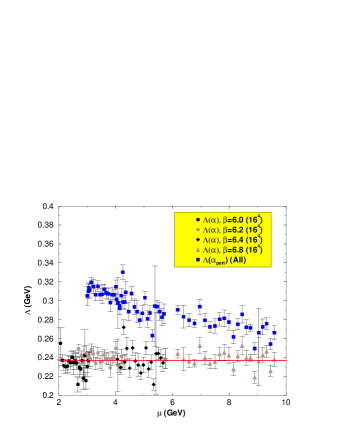
Figure 1: The upper plot shows $\Lambda_{\overline{\rm MS}}$ computed without power corrections while the lower plot shows $\Lambda_{\overline{\rm MS}}$ computed form the perturbative contribution to $\alpha_{s}$ once the power correction has been substracted, eq. (1) .

2.1 Power corrections and OPE

What can be the theoretical reason for these large power corrections ? In the theoretical framework of OPE a quadratic power requires a condensate of a dimension-two operator. Since we are working in the Landau gauge, such an operator exists: $<A_{\mu}A^{\mu}>$. Interestingly enough it is the only dimension two candidate for a vacuum expectation value in the Landau gauge.

We start from the OPE expansion of both the gluon propagator [6] and the symmetric three-gluon Green function, keeping only the relevant terms:

$$T\left(\widetilde{A}_{\mu}^{a}(-p)\widetilde{A}_{\nu}^{b}(p)\right)=(c_{0})^{ab}_{\mu\nu}(p)+\cdots$$ (3)

$$+(c_{2})^{ab\mu^{\prime}\nu^{\prime}}_{\mu\nu a^{\prime}b^{\prime}}(p)\ :A_{\mu^{\prime}}^{a^{\prime}}(0)\ A_{\nu^{\prime}}^{b^{\prime}}(0):+\cdots$$

$$T\left(\widetilde{A}_{\mu}^{a}(p_{1})\widetilde{A}_{\nu}^{b}(p_{2})\widetilde{A}_{\rho}^{c}(p_{3})\right)=\ (d_{0})^{abc}_{\mu\nu\rho}(p_{1},p_{2},p_{3})\cdots$$ (4)

$$+(d_{2})^{abc\mu^{\prime}\nu^{\prime}}_{\mu\nu\rho a^{\prime}b^{\prime}}(p_{1},p_{2},p_{3}):A_{\mu^{\prime}}^{a^{\prime}}(0)\ A_{\nu^{\prime}}^{b^{\prime}}(0):+\cdots$$

The Wilson coefficients depend on the renormalization scale. The leading coefficients, $c_{0}(\mu)$ and $d_{0}(\mu)$ are exactly the perturbative estimate of the considered Green functions which is known to three loops. The first subleading coefficients $c_{2}(\mu)$ and $d_{2}(\mu)$ are proportional to $1/\mu^{2}$ for dimensional reasons and they also depend logarithmically on the renormalization scale. We have computed to the leading logarithms approximation the anomalous dimensions of these coefficients and that of the $A^{2}$ operator.

We have then performed the following test of OPE: A simultaneous fit was first done of the two-point Green function and of $\alpha_{s}$ deduced from the symmetric three-point Green functions computed on the lattice. We have used the known dependence of the Wilson coefficient on the scale but, at this stage, fitted two different values for $<A^{2}>$. We then check the consistency of the resulting values of $<A^{2}>$.

$$\langle A^{2}\rangle_{prop}=(1.55(17){\rm GeV})^{2};\,\langle A^{2}\rangle_{alpha}=(1.9(3){\rm GeV})^{2}$$

$$\frac{\sqrt{\langle A^{2}\rangle_{alpha}}}{\sqrt{\langle A^{2}\rangle_{prop}}}\ =\ 1.21(18);\,\Lambda_{\overline{\rm MS}}=233(28){\rm MeV}$$

The two fitted values of $<A^{2}>$ agree within one standard deviation. This is a quite interesting result which tends to confirm the hypothesis that the $A^{2}$ condensate is at the origin of the power corrections. It is interesting to stress that if we use only the two loops formulae for the leading coefficients the fitted condensates differ by more than twenty standard deviations. This is a lesson for the use of OPE: if the leading coefficients are not expanded far enough in perturbation the OPE cannot be applied.

2.2 OPE for the asymmetric three-gluon Green function

OPE is more tricky to apply to the asymmetric Green function because of the presence of a zero momentum gluon. To be short, this mixes up the distinction between hard and soft gluons which is at the basis of the OPE approach. The issue has been discussed in [7]. Strictly speaking OPE applied to this operator introduces other operators than the identity and the $A^{2}$ considered above. One needs to consider gluon to vacuum matrix elements of operators with an odd number of gluon fields.

In order to be able to relate nevertheless the asymmetric three-gluon Green function measured on the lattice to the $A^{2}$ condensate the authors of [7] have introduced a “vacuum insertion hypothesis” (or factorization hypothesis) consisting in taking the matrix elements of three-gluon operators as the products of matrix elements of one gluon operators and of two-gluon operators. Then, the only non trivial matrix element is again $<A^{2}>$ and one can perform the same exercise as above. The combined fit of the propagator and the asymmetric $\alpha_{s}$ deduced from the asymmetric three-gluon Green function leads to:

$$\langle A^{2}\rangle_{prop}=\left(1.39(14){\rm GeV}\right)^{2};\,\langle A^{2}\rangle_{alpha}=\left(2.3(6){\rm GeV}\right)^{2}$$

$$\frac{\sqrt{\langle A^{2}\rangle_{alpha}}}{\sqrt{\langle A^{2}\rangle_{prop}}}\ =\ 1.7(3);\,\Lambda_{\overline{\rm MS}}=260(18){\rm MeV}$$

The agreement between both estimates of
$<A^{2}>$ is less satisfactory than in the previous case, maybe due to the added assumption of factorization or to the necessity of going to four loops for the dominant coefficients.

As a conclusion, we would like to emphasize the role of lattices as a beautiful tool to study the QCD vacuum and in particular the vacuum condensates and also to test the practical applicability of OPE. Notice also [8] that there is a good evidence for power corrections in the gluon Green functions computed with dynamical quarks.

3 Acknowledgments

This work was supported by the European Community’s Human potential programme under HPRN-CT-2000-00145 Hadrons/LatticeQCD.

References

- [1] B. Alles et al., NPB 502 (1997) 325; C. Parrinello, NPB (Proc. Suppl.) 63 (1998) 245.
- [2] Ph. Boucaud et al. JHEP 10 (98) 017.
- [3] D. Becirevic et al. PRD 60 (1999) 094509; PRD 61 (2000) 114508.
- [4] Ph. Boucaud et al. JHEP 0004 (2000) 006
- [5] S. Capitani et al., Nucl. Phys. Proc. Suppl. 63 (1998) 153; Nucl. Phys. B544 (1999) 669.
- [6] Ph. Boucaud et al., Phys. Lett. B493 (2000) 315-324; Phys. Rev. D63 (2001) 114003; hep-ph/0107278.
- [7] F. De Soto and J. Rodriguez-Quintero hep-ph/0105063.
- [8] Hervé Moutarde in these proceedings; Ph. Boucaud et al. hep-ph/0107278.