Measuring Cosmic Defect Correlations in Liquid Crystals

Abstract

From the theory of topological defect formation proposed for the early universe, the so called Kibble mechanism, it follows that the density correlation functions of defects and anti-defects in a given system should be completely determined in terms of a single length scale $\xi$, the relevant domain size, which is proportional to the average inter-defect separation $r_{av}$. Thus, when lengths are expressed in units of $r_{av}$, these distributions should show universal behavior, depending only on the symmetry of the order parameter, and space dimensions. We have verified this prediction by analyzing the distributions of defects/anti-defects formed during the isotropic-nematic phase transition in a thin layer in a liquid crystal sample. Our experimental results confirm this prediction and are in reasonable agreement with the results of numerical simulations.

The Big-Bang theory of the universe is well established by now, with most of the observations being in good agreement with the predictions of the model. Accurate measurements of the cosmic microwave background radiation (CMBR) have made cosmology into a precision science where competing models of the early universe are put to rigorous tests. One of the models which was very popular earlier for explaining the formation of structure in the universe, such as galaxies, clusters, and superclusters of galaxies, utilized the concept of the topological defects, in particular cosmic string defects [1]. Though recent CMBR anisotropy data is not in agreement with the predictions of topological defects based models of structure formation, it will be premature to completely reject these models due to various unresolved issues regarding these models [2]. Further, topological defects arise in many particle physics models of unification of forces, and their presence in the early universe can lead to other important consequences, such as, production of baryon number below electroweak scale, generating baryon number inhomogeneities at quark-hadron transition, etc. [3]. It is therefore important to deepen our understanding of how these defects form in the universe [4], and how they evolve. This paper relates to first of these issues.

There are numerous examples of topological defects in condensed matter systems, such as, flux tubes in superconductors, vortices in superfluid helium, monopoles and strings in liquid crystals, etc. It was long known that such defects routinely form during a phase transition. First detailed theory of formation of topological defects in a phase transition (apart from the usual equilibrium process of thermal production) was proposed by Kibble [5, 6] in the context of the early Universe. It is usually referred to as the Kibble mechanism. It was first suggested by Zurek [7] that some of the aspects of the Kibble mechanism can be tested in condensed matter systems, such as superfluid ⁴He. Indeed the basic physical picture of the Kibble mechanism applies equally well to a condensed matter system [8, 9, 4]. Using this correspondence, the basic picture of the defect formation was first observed by Chuang et al. in isotropic to nematic (I-N) transition in liquid crystal systems [10]. Formation and evolution of string defects was observed to be remarkably similar to what had been predicted for the case of the universe, apart from obvious differences such as the velocity of defects, time scales of the evolution of defect network etc. Subsequently, measurements of string density were carried out by observing strings formed in the first order I-N transition occurring via the nucleation of nematic bubbles in the isotropic background [11]. The results were found to be in good agreement with the prediction of the the Kibble mechanism. There have been other experiments, with superfluid helium [12], and with superconductors [13], where predictions of Kibble mechanism have been put to test. Yet another quantitative measurement was made of the exponent charactering the correlation between the defects and the anti-defects formed in the I-N transition in liquid crystals, with results in good agreement with the Kibble mechanism [14].

It is certainly dramatic that there is a correspondence between the phenomenon expected to have occurred in the early universe, during stages when its temperature was about $10^{29}$ K, with those occurring in the condensed matter systems at temperatures less than few hundred K. The important question is whether the observations/measurements performed in condensed matter systems provide rigorous tests of the theories being used to predict phenomenon in the early universe, or they simply provide an analogy with the case of the early universe, or at best, examples of other systems where similar theoretical considerations can be made for investigating defect formation. On the face of it, the differences between the two cases seem so profound that a rigorous test of theories underlying the phenomenon taking place in the early universe seems out of question within the domain of condensed matter systems. For example, the description of the matter, transformations between its various phases etc. in the early universe is given in terms of elementary particle physics models, which require the framework of relativistic quantum field theory. Indeed, typical velocities of particle, and even the topological defects formed in such transitions, are close to the velocity of light. On the other hand, in condensed matter systems non-relativistic quantum mechanics provides adequate description of most relevant systems. Typical velocities in such systems are extremely small in comparison. For example, in liquid crystals, typical velocity of string defects is of the order of few microns per second, completely negligible in comparison to the speed of light. Similarly, the value of string tension for the case of the universe is of the order of $10^{32}$ GeV² which is about $10^{18}$ tons/cm. In contrast, in condensed matter systems (say, in liquid crystals), the string tension is governed by the scale of the free energy of the order of $10^{-2}$ eV. Indeed, it is due to this extremely large string tension (i.e. mass per unit length) of cosmic string defects, that they were proposed to have seeded formation of galaxies, clusters of galaxies etc. via their gravitational effects. Clearly such effects are unthinkable for string defects in liquid crystals, or in superfluid helium etc.

Despite the fact that the two systems look completely dissimilar, it turns out, that there are ways in which specific condensed matter experiments can provide rigorous tests of the theories of cosmic defect formation. This can be done by identifying those predictions of the theory which show universal behavior. As we will discuss below there are several predictions of the Kibble mechanism which show universal behavior when expressed in terms of suitable length scale.

We first describe the basic physics of the Kibble mechanism [5, 6, 9]. For concreteness, we consider the case of a complex scalar order parameter $\phi$, with spontaneously broken U(1) symmetry (as in the case of superconductors, or superfluid ⁴He). The order parameter space (the vacuum manifold) is a circle $S^{1}$ in this case. In the Kibble mechanism, defects form due to a domain structure arising in a phase transition. This domain like structure arises from the fact that during phase transition, the phase $\theta$ of the order parameter field $\phi$ can only be correlated within a finite region. $\theta$ can be taken to be roughly uniform within a region (domain) of size $\sim\xi$, while varying randomly from one domain to the other. This situation is very natural to expect in a first order phase transition where the transition to the spontaneous symmetry broken phase happens via nucleation of bubbles. Inside a bubble, $\theta$ will be uniform, while $\theta$ will vary randomly from one bubble to another. Eventually bubbles grow and coalesce, leaving a region of space where $\theta$ varies randomly at a distance scale of the inter-bubble separation, thereby leading to a domain like structure. [In certain situations, e.g. when bubble wall motion is highly dissipative, effective domain size may be larger [15, 4]. In between any two adjacent bubbles (domains), $\theta$ is supposed to vary with least gradient. This is usually called the $geodesic~{}rule$ and arises naturally from the consideration of minimizing the gradient energy for the case of global symmetry. For gauge symmetry, situation is more complicated [16]. Geodesic rule may not hold in the presence of strong fluctuations [17, 18, 19]. Recently it has been shown [19], that a defect distribution very different from what is expected in the Kibble mechanism, may arise when defect formation is dominated by magnetic field fluctuations.]

The same situation happens for a second order transition where the orientation of the order parameter field is correlated only within a region of the size of the correlation length $\xi$. This again results in a domain like structure, with domains being the correlation volumes. We mention here that there are non-trivial issues in the case of a second order phase transition, in determining the appropriate correlation length for calculating the absolute initial defect density. It was first pointed out by Kibble [6] (see also, [4]) that the appropriate value of $\xi$ in this case should depend on the rate of phase transition. It was discussed by Zurek [8] that the appropriate value of $\xi$ should be determined by incorporating the effects of critical slowing down of the dynamics of the order parameter field near the transition temperature. The theory which takes into account of this (for second order transitions) is usually referred to as the Kibble-Zurek mechanism. Here, the absolute defect density is determined by critical fluctuations of the order parameter, and depends on details such as the rate of cooling of the system etc. For a discussion of these issues, see ref.[8]. We emphasize that these considerations of the details of the critical dynamics of the order parameter field during the phase transition are important in calculating the absolute defect density. However, defect density per domain is insensitive to these details.

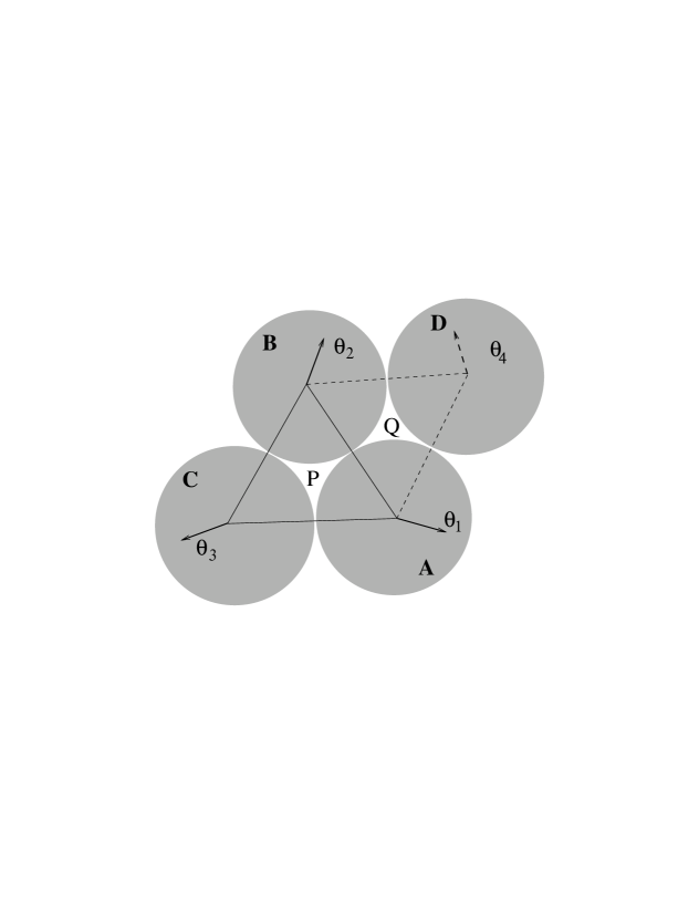
FIG. 1.: Defect formation due to coalescence of three domains.

For the U(1) case which we are discussing, string defects (vortices) arise at the junctions of domains if $\theta$ winds non trivially around a closed path going through adjacent domains. Consider a junction P of three domains, as shown in Fig.1. For simplicity, we show here domains as spheres (e.g. bubbles for a first order transition), with the centers of the three nearest bubbles forming an equilateral triangle. The values of $\theta$ in these three domains are, $\theta_{1}$, $\theta_{2}$ and $\theta_{3}$. One can show that with the use of the geodesic rule (i.e., the variation of $\theta$ in between any two domains is along the shortest path on the order parameter space $S^{1}$), a non-trivial winding of $\theta$ (i.e. by $\pm 2\pi$) along a closed path, encircling the junction P and going through the three domains A,B,C, will arise only when $\theta_{3}$ lies in the (shorter) arc between $\theta_{1}+\pi$ and $\theta_{2}+\pi$. Maximum and minimum values of the angular span of this arc are $\pi$ and 0, with average angular span being $\pi/2$. Since $\theta_{3}$ can lie anywhere in the circle, the probability that it lies in the required range is $p=(\pi/2)/(2\pi)=1/4$. Thus, we conclude [20] that the probability of vortex (or antivortex) formation at a junction of three domains (in 2-space dimensions) is equal to 1/4.

It is important to realize that in the above argument, no use is made of the field equations. Thus, whether the system is a relativistic one for particle physics, or a non-relativistic one appropriate for condensed matter physics, there is no difference in the defect production per domain. [This is so as long as the geodesic rule holds. As we have mentioned above, this may not be true when the field dynamics is dominated by fluctuations [17, 18, 19]. In those situations, defect production will be determined by some different processes, e.g. by a new flipping mechanism [17, 18], or by fluctuating magnetic fields [19], again, apart from the usual equilibrium thermal production.] Therefore, the expected number of defects per domain has universal behavior, in the sense that it only depends on the symmetry of the order parameter and the space dimensions. It is this universal nature of the prediction of defect density (number of defects per domain) in the Kibble mechanism which has been utilized to experimentally verify this prediction (which was originally given for cosmic defect production) in liquid crystal systems [11]. Note that absolute defect density does not show universal behavior since it depends on the domain size $\xi$. The entire dependence on the dynamical details of the specific system is through the single length scale $\xi$. Thus, when densities are expressed in length scale of $\xi$ the prediction acquires a universal character.

Kibble mechanism does not only predict the number density of defects. It also predicts a very specific correlation between the defects and anti-defects. Again, by focusing on specific quantities and choosing proper length scales, this prediction acquires a universal nature which can then be tested experimentally in condensed matter systems. This prediction is important as in many experimental situations it can provide the only rigorous test of the underlying theory of defect formation. This is for the following reason. As we have discussed above, prediction of defect density becomes universal only when expressed in the length units of the domain size. For a first order transition it can be done easily, if the average bubble diameter (assuming small variance in bubble sizes) can be experimentally determined, as in liquid crystal experiments in ref. [11]). However, this is a highly non-trivial problem for the case of second order transition (or for spinodal decomposition). For experimental situations with second order transition (type II superconductors, superfluid ⁴He), it has not been possible to make independent determination of the correlation length relevant for defect formation. All one can do is to measure absolute defect density, comparison of which to the prediction from theory becomes dependent on various details of phase transition, which determine the relevant correlation length [8].

Defect-anti-defect correlations, on the other hand, imply specific spatial distributions of defects, which are independent of the prediction of defect density. Within the framework of the Kibble mechanism, defect density distributions are expected to reflect defect-anti-defect correlations at the typical distance scales of a domain size. At the same time, typical inter-defect separation $r_{av}$, as given by $\rho^{-1/2}$, where $\rho$ is the average defect/anti-defect density, is directly proportional to the domain size $\xi$. From this, one can conclude that if defect and anti-defect distributions are expressed in terms of the average inter-defect separation $r_{av}$, then these should display universal behavior. The important point being that the same experiment yields the value of average inter-defect separation ($r_{av}=\rho^{-1/2}$), and the defect and anti-defect distributions are analyzed by using this length scale. Details such as the bubble size, or the relevant correlation length, therefore, become completely immaterial for testing the predictions regarding correlations.

To understand how this correlation between defects and anti-defects arises, let us go back to Fig.1. With the directions of arrows shown there (which denote values of $\theta$), we see that a defect (vortex with winding $+1$) has formed at P. Let us address the issue that, given that a defect has formed at P, how does the probability of a defect, or anti-defect, change in the nearest triangular region, say at Q. At Q, the three domains which intersect are A,B, and D. $\theta$ already has specific variation in A and B in order to yield a defect at P. From the point of view of Q, this variation in A and B is a partial winding configuration for an anti-vortex. With partial anti-winding present in A and B, it can be seen from Fig.1 that whatever be the value of $\theta$ in D, it is impossible to have a vortex at Q (i.e. $\theta$ winding by $+2\pi$ as we go around Q in an anti-clockwise manner). On the other hand, the probability of an antivortex formation at Q is 1/4 by straightforward repetition of the argument given above to calculate the probability of formation of a vortex or antivortex at a junction of three domains. This is the most dramatic example of correlation between defect and anti-defect formation. If we consider defect formation due to intersection of (say) four domains, this correlation still exists, that is close to a defect, formation of another defect is less likely (though not completely prohibited now) and formation of anti-defect is enhanced. This conclusion, about certain correlation in the formation of a defect and an anti-defect, is valid for other types of defects as well [21].

To see what this correlation implies, let us consider a two dimensional region $\Omega$ whose area is $A$ and whose perimeter L goes through $L/\xi$ number of elementary domains (where $\xi$ is the domain size). As $\theta$ varies randomly from one domain to another, one is essentially dealing with a random walk problem with the average step size for $\theta$ being $\pi/2$ (the largest step is $\pi$ and the smallest is zero). Thus, the net winding number of $\theta$ around L will be distributed about zero with a typical width given by $\sigma={1\over 4}\sqrt{L\over\xi}$, implying that $\sigma\propto A^{1/4}$ (see, ref. [22, 14, 9]). Assuming roughly uniform defect density, we get $\sigma\propto N^{1/4}$ (where $N$ is the total number of defects in the region $\Omega$), which reflects the correlation in the production of defects and anti-defects. In the absence of any correlations, the net defect number will not be as suppressed, and will follow Poisson distribution with $\sigma\sim\sqrt{N}$. In general one may write the following scaling relation for $\sigma$,

$$\sigma~{}=~{}C~{}N^{\nu}$$ (1)

The exponent $\nu$ will be 1/2 for the uncorrelated case and 1/4 for the case of the Kibble mechanism. Again, the prediction of $\nu=1/4$ is of universal nature, depending only on the symmetry of order parameter and space dimensions. An experimental measurement of this exponent was carried out in ref.[14]. The experimental value of $\nu$ was found in ref.[14] to be $\nu=0.26\pm 0.11$ which is in a good agreement with the predicted value of 1/4 from the Kibble mechanism, and reflects the correlated nature of defects and anti-defects.

The exponent $\nu$ does not give complete information about the correlation which arises between defects and anti-defects when they are produced via the Kibble mechanism. A more detailed understanding of the correlation can be achieved by calculating the density correlation function of the defects and anti-defects. Below, we first discuss theoretical prediction about this, and then describe the experimental measurements.

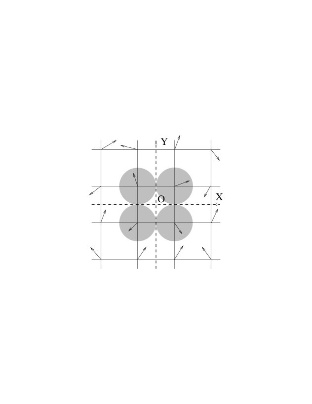
FIG. 2.: Defect formation due to coalescence of four elementary domains, forming a square lattice.

We have carried out the numerical simulation of defect formation via the Kibble mechanism for the square lattice case (instead of triangular case as shown in Fig.1) where defects will form at the intersection of four domains, see Fig.2. This is because we find slightly better agreement with the experimental results for the square lattice case. We will also quote results for the triangular lattice case. The probability $p$ of a defect or an anti-defect per square region (in Fig.2) is obtained to be 0.33. We start with a defect at the origin O of the coordinate system. We then calculate the density of anti-defects $\rho_{\bar{d}}(r)$, as well as the density of defects $\rho_{d}(r)$, as a function of the radial distance $r$ from the defect at the origin. For this, we count number of anti-defects (defects) in an annular region of width $\Delta r$ centered at distance $r$ from the origin, and divide this number by the area of the annular region. An average of these densities (at a given $r$) is taken by taking many realizations of the event of defect production. With density in the central square (which has a defect) appropriately normalized, this is the same as the density correlation function. As should be clear by now, all the dynamical details of the specific model are relevant only in determining the domain size $\xi$ (i.e., either the bubble diameter for a first order transition case, or the relevant correlation length for a second order transition case, or for spinodal decomposition). For the simulation, we take domain size to be unity, meaning that all lengths are measured in units of domain size. All remaining properties of the defect distributions should now display universal behavior, depending only on the symmetry of the order parameter (U(1) in this case), space dimensions (2 here), and, possibly, fundamental domain structure (square vs. triangular). Another important factor here is that there is no reason to expect that the defect/anti-defect will be exactly at the center of the square formed by the centers of the four bubbles (domains). In realistic situation, the defects can be anywhere in the elementary square, which in some sense represents the collision region of the four correlation domains (bubbles). However, since the correlation domains, by definition, have uniform order parameter, it should be increasingly unlikely that the defect is far from the center of the collision region (i.e. away from O). To take into account of these physical considerations, we have allowed the position of defects/anti-defects to float within a square with an approximately Gaussian probability distribution, centered in the middle of the square, with varying width. By changing the width of this distribution we can change from almost centered defects, to defects with uniform probability in the elementary square region.

With this picture, and with a defect being in the central square, we know that the probability of anti-defect formation should be enhanced in the nearest squares, while the probability of defect formation should be suppressed in these regions. These defects/anti-defects cannot be too close to the central defect as that would imply variation of the order parameter at distance scales much smaller than $\xi$. One therefore expects that both $\rho_{\bar{d}}(r)$ and $\rho_{d}(r)$ will be almost zero for $r<<\xi$ (discounting the central defect at O). Both densities will rise as $r$ increases. At a distance of about $r\sim\xi$, one expects a peak in $\rho_{\bar{d}}(r)$. The height of this peak will determine the suppression in $\rho_{d}(r)$ (compared to the asymptotic value) at that point.

For $r\geq 2\xi$ one expects both distributions to approach the average density expected asymptotically. This conclusion may appear surprising as one might have expected that increased anti-defect probability in the nearest square may imply suppressed anti-defect probability in the next-nearest square etc., leading to a damped oscillatory behavior of $\rho_{\bar{d}}(r)$ and $\rho_{d}(r)$ (similar to density correlation function for a liquid). The reason that this does not happen here is simple, and again, intrinsic to the Kibble mechanism. Recall that the anti-defects were enhanced (and defects suppressed) in the squares nearest to the central square because for each of these four squares, two out of four vertices had $\theta$ common to the central square which already had a defect. The probability of defects/anti-defects in these squares was, therefore, affected by the presence of defect in the central square. In contrast, $\theta$ at three vertices of the next nearest (corner) squares, and at all vertices further away, are completely random. This implies that the probability of defect and anti-defect must be equal in all such regions, leading to flattening of $\rho_{\bar{d}}(r)$ and $\rho_{d}(r)$ for $r\geq 2\xi$. As we will see below, this theoretical reasoning is well born out by the results of the simulations, and is consistent with the experimental results, within error bars.

We have explained above that this analysis of defect-anti-defect correlations does not require the knowledge of domain size. In fact, the power of this technique is best illustrated in those experimental situations where domains are not identifiable (as in the experiments explained below). The length scale $\xi$ is, therefore, not a convenient choice from this point of view. We, instead, will use the inter-defect separation $r_{av}$ to define our length scale. If the probability of defect formation per (square) domain is $p$, then $r_{av}$ and $\xi$ are related in the following manner.

$$r_{av}={\xi\over\sqrt{p}}$$ (2)

In our experiment, we have tried to record the defect distributions as soon as defects form. Note that even if some evolution of defect network occurs by coarsening of domains, Eq.2 still holds. Coarsening of domains only makes the effective correlation domain size $\xi$ larger. Since the probability $p$ (defects per domain) is also of universal nature, it follows from Eq.(2) that the distributions $\rho_{\bar{d}}(r)$ and $\rho_{d}(r)$ will still show universal behavior if $r$ is measured in the units of $r_{av}$. As $r_{av}$ can be directly measured for a given defect distribution, without any recourse to underlying domain structure, we will use it as defining the unit of length. In this unit, the peak in $\rho_{\bar{d}}(r)$ will be expected to occur at $r=\sqrt{p}\simeq 0.57$ with $p=0.33$ for the square lattice case. (This is when the order parameter space is $S^{1}$, which, as we will discuss below, is the case for our experiment). By $r=2\sqrt{p}\simeq 1.14$, both densities will be expected to flatten out to the asymptotic value of 0.5. The asymptotic value of $\rho_{d}$ and $\rho_{\bar{d}}$ is 0.5 since by definition the unit length $r_{av}$ is the average separation between defects/anti-defects. The height of the peak for $\rho_{\bar{d}}$ (at $r\simeq 0.57$) depends on the weight factor for centering the defects/anti-defects inside square regions. This is simply because perfectly centered defects/anti-defects will lead to large contributions when centers of the squares fall inside the annular regions for calculating densities. While for neighboring values of $r$, their contributions will be zero. When defects/anti-defects positions are floated, then the contributions are averaged out. We find that the height of the peak varies from about 1.2 for perfectly centered defects/anti-defects to about 0.75 for the case when defects/anti-defects positions are uniformly distributed inside a square. When comparing with the experimental results, we choose the weight factor appropriately so that the height of the peak in $\rho_{\bar{d}}$ from simulation is similar to the one obtained from experiment. (It will be interesting to investigate the physics contained in the peak height resulting from this weight factor for centering the defects in a square, which may depend on the interactions between defects/anti-defects.)

If we take the thickness of the annular region $\Delta r$ (for calculating densities) to be about the domain size (i.e., 0.57 in units of $r_{av}$), then one can relate the suppression in $\rho_{d}$ at $r=\sqrt{p}\simeq 0.57$ to the height of the peak in $\rho_{\bar{d}}$ at that position. This is done as follows. Note that the values of $\theta$ at all the outer 12 vertices of the 8 squares, bordering the central square, are completely random (i.e. they are not constrained by the fact that there is a defect in the central square). Let us consider the distribution of the net winding along the large square shaped path going through all these 12 vertices. Repetition of the earlier argument (in writing Eq.(1)) shows that this net winding should be distributed about the value zero, (and should have a typical width proportional to $\sqrt{12}$, but this part is not relevant here). Thus, average number of defects $n_{d}$ inside this large square should be same as the average number of anti-defects $n_{\bar{d}}$. However, we are given that the central square always has one defect. With the area of each domain $\xi^{2}=p$ in the units of $r_{av}$, this directly leads to the relation between $\rho_{d}$ and $\rho_{\bar{d}}$ at $r\simeq 0.57$ to be

$$\rho_{d}(r=0.57)=\rho_{\bar{d}}(r=0.57)-{1\over 8p}~{}\simeq~{}\rho_{\bar{d}}(r=0.57)-0.39,$$ (3)

for $p=0.33$. Here, we have approximated the densities at $r\simeq 0.57$ by dividing the expected number of defects (anti-defects) in the eight squares bordering the central square, by the total area of these squares, even though the corner squares are somewhat further away. (If one accounts for the larger distance of these corner squares, and that defects and anti-defects are equally probably there, then the suppression in $\rho_{d}(r=0.57)$ would be larger.)

Our experiments have been carried out using nematic liquid crystals. For uniaxial nematic liquid crystals (NLC) the orientation of the order parameter in the nematic phase is given by a unit vector (with identical opposite directions) called the director. The order parameter space is $RP^{2}(\equiv S^{2}/Z_{2})$, which allows for string defects with strength 1/2 windings. Due to birefringence of NLC, when the liquid crystal sample is placed between crossed polarizers, then regions where the director is either parallel, or perpendicular, to the electric field ${\vec{E}}$, the polarization is maintained resulting in a dark brush. At other regions, the polarization changes through the sample, resulting in a bright region. This implies that for a defect of strength $s$, one will observe $4s$ dark brushes [23]. If the cross-polarizer setup is rotated then brushes will rotate in the same (opposite) direction for positive (negative) windings. Equivalently, if the sample is rotated between fixed crossed polarizers, then brushes do not rotate for +1 winding while they rotate in the same direction (with twice the angle of rotation of the sample) for $-$1 winding. We have used this method to determine the windings.

We now describe our experiment. We observed isotropic-nematic (I-N) transition in a tiny droplet (size $\sim$ 2-3 mm) of NLC $4^{\prime}$-Pentyl-4-biphenyl-carbonitrile (98% pure, purchased from Aldrich Chem.). The sample was placed on a clean, untreated glass slide and was heated using an ordinary lamp. The I-N transition temperature is about 35.3 ⁰C. Our setup allowed the possibility of slow heating, and cooling, by changing the distance of the lamp from the sample. We observed the defect production very close to the transition temperature (in some cases we had some isotropic bubbles co-existing with the nematic layer containing defects). For the observations, we used a Leica, DMRM microscope with 20x objective, a CCD camera, and a cross-polarizer setup, at the Institute of Physics, Bhubaneswar. Phase transition process was recorded on a standard video cassette recorder. The images were photographed directly from a television monitor by replaying the cassette.

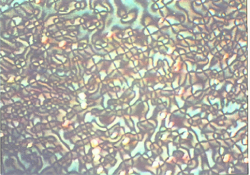
FIG. 3.: Network of strength one defects and anti-defects formed in I-N transition. Crossing of brushes denotes defects with winding $\pm$ 1. Size of the image is about 0.45 mm $\times$ 0.32 mm.

The I-N transition is of first order. When the transition proceeds via nucleation of bubbles, we observe long horizontal strings (as in ref. [11]), which are not suitable for our present analysis. We selected those events where the transition seems to occur uniformly in a thin layer near the top of the droplet (possibly due to faster cooling from contact with air). The depth of field of our microscope was about 20 microns. All the defects in the field of view were well focused suggesting that they formed in a thin layer, especially since typical inter-defect separation was about 10 - 40 microns. (For us, the only thing relevant is that the layer be effectively two dimensional over distances of order of typical inter-defect separation). Also, the transition happened over the entire observation region roughly uniformly, suggesting that a process like spinodal decomposition may have been responsible for the transition. This resulted in a distribution of strength $\pm 1$ defects as shown in the photograph in Fig.3. Points from which four dark brushes emanate correspond to defects of strength $\pm$ 1. Due to resolution limitation the crossings here do not appear as point like. It is practically impossible to use the technique of rotation of brushes to identify every winding in situations such as shown in Fig.3 due to very small inter-defect separation (resulting from high defect density), as well as due to rapid evolution of the defect distribution.

We have developed a particular technique for determining individual windings of defects in situations like Fig.3 where one only needs to determine the winding of one of the defects by rotation in a cross polarizer setup. Windings of the rest of the defects can then be determined using topological arguments, see ref. [14] for details of this technique. Further, as explained in ref. [14], the anchoring of the director at the I-N interface [24] forces the director to lie on a cone, with the half angle equal to about 64⁰. This forces the order parameter space there to become effectively a circle $S^{1}$, instead of being $RP^{2}$, with the order parameter being an angle between 0 and $2\pi$. Only defects allowed now are with integer windings which is consistent with the fact that no strength 1/2 defects are seen in our experiment [14]. Therefore the prediction of the Kibble mechanism for the U(1) case, as described above, are valid for this case, with the picture that a domain structure near the I-N interface is responsible for the formation of integer windings (see, ref. [14] for detailed discussion of these points).

After identifying the windings of all defects (wherever possible) in a picture, we note down the positions (x-y coordinates) of each defect and anti-defect in the picture. We then determine the average defect/anti-defect density $\rho$. With the average inter-defect separation $r_{av}$ being $\rho^{-1/2}$, we convert all coordinate distances into scaled distances by dividing with $r_{av}$. We then choose one defect as the origin, making sure that the defect is at least 1 unit (with unit length being $r_{av}$ now) away from the boundary of the picture. Density of defects $\rho_{d}(r)$ as well as density of anti-defects $\rho_{\bar{d}}(r)$ is now calculated at each $r$ (at step size of $\Delta r$) by counting number of defects (anti-defects) within an annular region of thickness $\Delta r$ centered at $r$. Different values of $\Delta r$ are used to to get least possible statistical fluctuations, while at the same time, retaining the structure of the peak etc. Same $\Delta r$ is used in numerical simulation for comparison with the experimental data. We will present results for $\Delta r=0.25$ (in the units of $r_{av}$). The calculation is repeated by taking other defects as origins, and an average of densities (at a given value of $r$) is taken to determine final values of $\rho_{d}(r)$ and $\rho_{\bar{d}}(r)$. To increase the statistics, an average of the distributions is taken by combining the results of all pictures. Different pictures have very different values of $r_{av}$, ranging from about 5 microns to about 50 microns. However, when expressed in the units of $r_{av}$, the densities $\rho_{d}$ and $\rho_{\bar{d}}$ show similar behavior for all the pictures (at least those ones which had significant statistics). In all, we have analyzed 17 pictures, with total number of defects and anti-defects being 833.

FIG. 4.: Solid plots show simulation results for defect density $\rho_{d}(r)$ (top figure) and anti-defect density $\rho_{\bar{d}}(r)$ (bottom figure). Stars show the experimental data.

Fig.4 shows the results. Solid plots shows the results of the simulations. Antidefect distribution clearly shows a peak at $r\simeq 0.6$ as expected from the Kibble mechanism. Defect density is suppressed in that region at $r\simeq 0.6$, with the simulation results not too different from the expected suppression, i.e. $\rho_{d}\simeq\rho_{\bar{d}}-0.4\simeq 0.5$ (with $p\simeq 0.33$ and $\rho_{\bar{d}}(r=0.57)\simeq 0.9$). (As we mentioned above, accounting for difference between the corner 4 squares from the nearest 4 squares would have led to larger suppression for $\rho_{d}(r=0.57)$.) As expected, both densities reach asymptotic values by $r\sim 1$. The regular oscillations in the densities is due to the regular lattice structure of the simulations, with defects and anti-defects remaining close to the centers of the domains. If defects/anti-defects are assumed to be strictly at the centers of the domains, then the oscillations in $\rho_{\bar{d}}(r)$ and $\rho_{d}(r)$ are even more pronounced and regular. At the other extreme, if the positions of defects/anti-defects are taken to be uniform within respective domains, then these oscillations completely disappear, except for the prominent peak in $\rho_{\bar{d}}$ at $r\simeq 0.6$. Here we have taken an intermediate case with the positions of defects/anti-defects weighted by a Gaussian centered at the middle of the elementary square (so that the peak height is similar to the one obtained from the experiment, as discussed above).

Stars show the experimental values. The error bars have been calculated by taking the error in the count $n$ of defects or anti-defects within an annular strip (of the same thickness $\Delta r=0.25$ used for the simulation) to be $\sqrt{n}$. The peak in the data points of anti-defect density is prominent, and so is the suppression in the defect density for $r<1.0$. Data on defect density seems to be in a reasonably good agreement with the simulation results, especially the amount of suppression for $r<1$. The position of the anti-defect peak from experimental data seems to be shifted by about 0.25 on right, as compared to the peak from the simulation. With the statistics we have at present, it is not possible to resolve whether this shift is genuine, or whether it is due to statistical fluctuations. We have done following checks to address this point. Instead of square elementary domains, if we take triangular domains in the simulation (with due account of geometrical factors in Eq.(2) etc.), we find the simulation peak at about $r\simeq 0.4$, that is, slightly further shifted towards left compared to the experimental peak. This is consistent with the findings in ref.[14] where it was found that experimental data favored square elementary domains. Again, just as in the case in ref.[14], data in the present analysis also does not have enough statistics to make definitive statements about this issue of preferred shape of elementary domains. Even though, it is possible that the simulation peak may shift further to right for elementary domains with larger number of sides (which increases the probability $p$), it is clear from Eq.2 that the position of the peak will always remains at $r<1$ (in units of $r_{av}$).

With a smaller set of data we had seen that the shift between experimental peak and the simulation peak was larger. With the inclusion of all defects/anti-defects (which could be analyzed using our techniques), the shift reduced, suggesting that it is possible that the shift may reduce further if larger data is available. Even at present, the shift between the two peaks is relatively small. In fact the shift is about the same as the smallest separation between defects and/or anti-defects which we have found in our experiments.

The observation of the peak in $\rho_{\bar{d}}(r)$, near $r\simeq 0.8$, is roughly in accordance with the theoretical prediction. What is remarkable is that the data shows a prominent peak near the position where it is expected, and at the same time shows suppression in defect density by about the right amount, at the same point. At large $r$ there is not sufficient statistics to say whether the densities approach the asymptotic values at $r\simeq 1.1$, though the data is certainly consistent with this (in the sense that there are no other prominent peaks visible, and the fluctuations are randomly distributed about the asymptotic value). (We note here, that it is intriguing that similar structure of plots has been seen for the scaled radial distribution functions of islands formed on a single crystal substrate [25]. It will be interesting to explore of any possible connection between the two cases.)

We conclude by stressing that our measurements of the density correlation function of defects and anti-defects provide rigorous tests of the theory of cosmic defect formation, as well as defect formation in condensed matter systems. For a liquid crystal system, $r_{av}$ is about 10 microns, while $r_{av}$ will be about $10^{-30}$ cm for cosmic defects (those formed at Grand Unified Theory transition). However, when expressed in the scaled length $r$ (by dividing by $r_{av}$), one expects in both cases, a peak in anti-defect density at $r\simeq 0.6$ and flattening out by $r\simeq 1$ (for U(1) case and for 2 dimensional cross-sections of defect networks). Similarly defect density is predicted to be suppressed by a calculable factor at $r\simeq 0.6$, again flattening out by $r\simeq 1$. Experimental data verifies both these predictions, though fluctuations due to small statistics are large. It is clearly desirable to be able to carry out experimental analysis with significantly larger data set in order to improve the error bars, so that more definitive statements can be made about the comparison between theory and experiments, (e.g., about the apparent shift in the peak position). What is very encouraging and remarkable is that by appropriately focusing on predictions of theory of cosmic defect formation which acquire universal behavior by suitable change of length scales, one is able to rigorously test these theories in ordinary condensed matter experiments.

We are very thankful to Soma Dey, Sanatan Digal, Soma Sanyal, Supratim Sengupta, and Shikha Varma, for useful discussions and comments. AMS would like to acknowledge the hospitality of the Physics Dept. Univ. of California, Santa Barbara while the paper was being written. His work at UCSB was supported by NSF Grant No. PHY-0098395.

REFERENCES

- [1] A. Vilenkin and E.P.S. Shellard, Cosmic strings and other topological defects, (Cambridge University Press, Cambridge, 1994).
- [2] R. Durrer, astro-ph/0003363; C.R. Contaldi, astro-ph/0005115; L. Pogosian, astro-ph/0009307; A. Albrecht, astro-ph/0009129.
- [3] R. H. Brandenberger, A.C. Davis, M. Hindmarsh, Phys. Lett. B263, 239 (1991); R. Brandenberger, A.C. Davis, Mark Trodden, Phys. Lett. B335, 123 (1994); B. Layek, S. Sanyal and A.M. Srivastava, hep-ph/0107174; B. Layek, S. Sanyal and A.M. Srivastava, Phys. Rev. D63, 083512 (2001).
- [4] Formation and interactions of topological defects, Edited by, A.C. Davis and R. Brandenberger, Proceedings of NATO Advanced Study Institute, 1994, (Plenum, New York).
- [5] T.W.B. Kibble, J. Phys. A9, 1387 (1976).
- [6] T.W.B. Kibble, Phys. Rept. 67, 183 (1980).
- [7] W.H. Zurek, Nature 317, 505 (1985).
- [8] W.H. Zurek, Phys. Rep. 276, 177 (1996); P. Laguna and W.H. Zurek, Phys. Rev. Lett. 78, 2519 (1997); A. Yates and W.H. Zurek, Phys. Rev. Lett. 80, 5477 (1998); L.M.A. Bettencourt, N.D. Antunes, and W.H. Zurek, Phys. Rev. D62, 065005 (2000).
- [9] A. Rajantie, hep-ph/0108159.
- [10] I. Chuang, R. Durrer, N. Turok and B. Yurke, Science 251, 1336 (1991).
- [11] M.J. Bowick, L. Chandar, E.A. Schiff and A.M. Srivastava, Science 263, 943 (1994).
- [12] P.C. Hendry et al, Nature (London) 368, 315 (1994); V.M.H. Ruutu et al, Nature (London) 382, 334 (1996); M.E. Dodd et al, Phys. Rev. Lett. 81, 3703 (1998), see also, G.E. Volovik, Czech. J. Phys. 46, 3048 (1996).
- [13] R. Carmi, E. Polturak, and G. Koren, Phys. Rev. Lett. 84, 4966 (2000).
- [14] S. Digal, R. Ray, and A.M. Srivastava, Phys. Rev. Lett. 83, 5030 (1999).
- [15] J. Borrill, T.W.B. Kibble, T. Vachaspati, and A. Vilenkin, Phys. Rev. D52, 1934 (1995); A. Ferrera, Phys. Rev. D57, 7130 (1998).
- [16] S. Rudaz and A. M. Srivastava, Mod. Phys. Lett. A8, 1443 (1993); R.H. Brandenberger and A.C. Davis, Phys. Lett. B332, 305 (1994); T.W.B. Kibble and A. Vilenkin, Phys. Rev. D52, 679 (1995).
- [17] S. Digal and A.M. Srivastava, Phys. Rev. Lett. 76, 583 (1996); S. Digal, S. Sengupta and A.M. Srivastava, Phys. Rev. D55, 3824 (1997); ibid. D56, 2035 (1997); ibid D58, 103510 (1998).
- [18] E.J. Copeland and P.M. Saffin, Phys. Rev. D54, 6088 (1996).
- [19] M. Hindmarsh and A. Rajantie, Phys. Rev. Lett. 85, 4660 (2000); G.J. Stephens, L.M.A. Bettencourt, and W.H. Zurek, cond-mat/0108127.
- [20] T. Vachaspati, Phys. Rev. D44, 3723 (1991).
- [21] A.M. Srivastava, Phys. Rev. D43, 1047 (1991).
- [22] T. Vachaspati and A. Vilenkin, Phys. Rev. D30, 2036n (1984).
- [23] S. Chandrasekhar and G.S. Ranganath, Adv. Phys. 35, 507 (1986).
- [24] S. Faetti and V. Palleschi, Phys. Rev. A30, 3241 (1984).
- [25] V. Bressler-Hill, S. Varma, A. Lorke, B. Z. Nosho, P. M. Petroff, and W. H. Weinberg, Phys. Rev. Lett. 74, 3209 (1995).