Big Bang Nucleosynthesis Constraints on Bulk Neutrinos

Abstract

We examine the constraints imposed by the requirement of successful nucleosynthesis on models with one large extra hidden space dimension and a single bulk neutrino. We first use naive out of equilibrium conditions to constrain the size of the extra dimensions and the mixing between the active and the bulk neutrino. We then use the solution of the Boltzman kinetic equation for the thermal distribution of the Kaluza-Klein modes and evaluate their contribution to the energy density at the BBN epoch to constrain the same parameters.

I Introduction

There has been a great deal of interest and activity in the last two years on the possibility that there may be one or more extra space dimensions in nature which have sizes of order of a millimeter[1]. This has been driven by the realization that string theories provide a completely new way to view a multidimensional space time in terms of a brane-bulk picture, where a brane is lower dimensional space-time manifold that contains known matter and forces and the bulk consists of the brane plus the rest of space dimensions where only gravity is present. The resulting picture replaces Planck scale by the string scale as the new fundamental scale beyond the standard model. The relation between the familiar Planck scale and the string scale $M_{*}$ is given by the formula[1]

$$M^{2}_{P\ell}~{}=~{}M^{2+n}_{*}R_{1}R_{2}R_{3}\cdot\cdot\cdot R_{n}$$ (1)

For $R_{1}\simeq R_{2}=R$ and $R_{3}\simeq R_{4}\simeq\cdot\cdot=M^{-1}_{*}$, this relation leads to $R\simeq$ millimeter for $M_{*}\simeq$TeV. The fact that the familiar inverse square law of gravity allows for the existence of such sub-millimeter size extra dimensions made these models interesting for phenomenology[2]. An added attraction was the fact that a whole new set of particles are present at the TeV scale making such theories accessible to collider tests. Furthermore since there are no high scales in the theory, there is no hierarchy problem between the weak and the Planck scale; this provided an alternative approach (resolution ?) to the familiar gauge hierarchy problem. Obviously, the picture would become much more interesting if collider experiments such as those planned at LHC or Tevatron fail to reveal any evidence for supersymmetry.

Even though these models present an attractive alternative to the standard grand unification scenarios, there are two arenas where the simplest TeV string scale, large extra dimension models lead to problems: (i) one has to do with understanding neutrino masses and (ii) second is in the domain of cosmology and astrophysics.

The reason for the first is that the smallness of neutrino masses is generally thought to be understood via the seesaw mechanism[3], the fundamental requirement of which is the existence of a scale $\geq 10^{11}$ or $10^{12}$ GeV, if the neutrino masses are in the sub eV range. Clearly this is a much higher scale than $M_{*}$ of the TeV scale models. A second problem is that if one considers only the standard model group on the brane, operators such as $LHLH/M_{*}$ could be induced by string theory in the low energy effective Lagrangian. For TeV scale strings this would obviously lead to unacceptable neutrino masses.

In the domain of cosmology, the problems are related to the existence of the Kaluza-Klein (KK) tower of gravitons generally which lead to overclosure of the Universe unless the highest temperature of the universe is about an MeV[4]. This can not only cause potential problems with big bang nucleosynthesis but also with understanding of the origin of matter, inflation etc. There are also arguments based on SN1987A observations that require that $M_{*}\geq 50-100$ TeV[5].

The neutrino mass problem was realized early on and a simple solution was proposed in ref.[6]. The suggestion was to postulate the existence of one or more gauge singlet neutrinos, $\nu_{B}$, in the bulk which couple to the lepton doublets in the brane. We will call this the bulk neutrino. After electroweak symmetry breaking, this coupling can lead to neutrino Dirac masses, which are of order $hv_{wk}M_{*}/M_{P\ell}$. This leads to $m_{\nu}\simeq 10^{-4}$ eV. The dominant nonrenormalizable terms have to be forbidden in this model. The simple way to accomplish this is to assume the existence of a global B-L symmetry in the theory. The only difficulty with this assumption is that string theories are not supposed to have any global symmetries and one has to find a way to generate an effective B-L symmetry at low energies without putting it in at the beginning.

There is an alternative scenario for neutrino masses[7, 8], where one abandons the TeV string scale but maintains one large extra dimension and avoids the problem associated with nonrenormalizable operators. The relation in Eq. (1) then gets modified to the form

$$M^{2}_{P\ell}~{}=~{}M^{3}_{*}R$$ (2)

Since the string scale in these models is in the intermediate range i.e. $10^{9}$ GeV or so, the cosmological overclosure problem is avoided. The active neutrino masses in such models could arise from seesaw mechanism or from the presence of bulk neutrinos. The inclusion of the bulk neutrino however brings in new neutrinos into the theory which can be ultralight (i.e. $R^{-1}$, where $R$ is the size of the large extra dimension) and can play the role of the sterile neutrino, which may be required e.g. if the LSND results are confirmed.

Both the above approaches have the common feature that they introduce a bulk neutrino into the theory, which is equivalent in the brane to an infinite tower of sterile neutrinos. All of these neutrino modes mix with the active neutrinos in the process of mass generation[6, 7]. For extra dimension size of order $\sim$ mm, the KK modes have masses typically of order $nR^{-1}\sim n\times 10^{-3}$ eV or so, where $n=0,1,2,3,\cdot\cdot\cdot$. The presence of this dense tower of extra sterile states coupled to the known neutrinos leads to a variety of new effects in the domain of particle physics[9] and cosmology[10, 11, 12], which in turn impose constraints on the allowed size of the extra dimensions. In this paper, we focus on the cosmological constraints that may arise from the contribution of the neutrino states to big bang nucleosynthesis.

The constraints from big bang nucleosynthesis on bulk neutrinos were considered in Ref.[10, 11], where the cases of $\geq$ 2 extra dimensions were discussed. As it was noted there, light KK modes of the bulk neutrinos could easily be produced in the early universe, when temperature is of order an MeV or more. Thus, there is the danger that they could make large contribution to the energy density of the universe at the epoch of big bang nucleosynthesis (BBN) and completely destroy our current, successful understanding of the primordial abundance of $He^{4}$, $D$ and $Li^{7}$[13]. In particular, present abundance data from metal poor stars is well understood provided we do not have more than one extra active neutrino in the theory in addition to the three known ones i.e. $(\nu_{e},\nu_{\mu},\nu_{\tau})$. By the same token, if there are extra species of neutrinos that do not have conventional weak interactions, their masses and mixings to known neutrinos must obey severe constraints[14].

Our goal in this paper is to revisit this issue in the context of models with only one large extra dimension. The first reason for undertaking this analysis is that the class of models with intermediate string scale $\sim 10^{9}$ Gev and one large extra dimension[7, 8] have certain theoretical advantages and they are also free of the cosmological and astrophysical problems that seem to plague the TeV scale models. Secondly, the number of KK modes in this case are much fewer than models with larger number of large extra dimensions and therefore, one would expect the constraints to be somewhat less restrictive.

We also wish to emphasize that one large extra dimension could also occur in models with string scale in the 100 TeV range, where one can satisfy the Planck-scale-string-scale relation in Eq. (1), if the compactification is not isotropic, e.g. for a string scale of 100 TeV, if two extra dimensions have sizes $r\sim$ GeV^-1 and one has $R\sim$ millimeter, i.e. $M^{2}_{P\ell}=M^{5}_{*}Rr^{2}$.

We organize this paper as follows: in sec II, we discuss the constraints of big bang nucleosynthesis on the size of the extra dimension in the presence of the bulk neutrino and the mixing of the bulk neutrino to the active one using simple out of equilibrium condition. In section III, we use Boltzman equation to study the generation of the bulk neutrinos from active neutrino interactions in the early universe and find the constraint of BBN on the same parameters as in sec. II. The numerical calculations leading to our final results are given in sec.IV. In appendix A, we explain the details of the out of equilibrium condition for the KK modes of the neutrino.

II Constraints from out of equilibrium condition

The class of models, we will be interested in, are assumed to have one large extra dimension with a single bulk neutrino $\nu_{B}$, which means that masses of the KK modes of $\nu_{B}$ are integer multiples of the basic scale $\mu\equiv R^{-1}\sim 10^{-3}$ eV. This is one of the parameters that we expect the BBN discussion to constrain. The second parameter is the mixing of the KK modes with the active brane neutrinos, e.g. $\nu_{e}$. It is true in both classes of models i.e. both TeV and intermediate scale type,[6, 8] that the typical mixing parameter of the active neutrino to the nth KK mode scales like $\theta_{en}\simeq\frac{\theta}{n}$, in the range of interest for phenomenology. The parameter $\theta$ depends on the size of the extra dimension and other parameters of the theory such as the weak scale etc. For instance, in TeV scale models[6], one has $\theta\sim\frac{\sqrt{2}hv_{wk}M_{*}R}{M_{P\ell}}$, whereas in the local B-L models, the relation is $\theta\simeq\frac{hv_{wk}v_{R}R}{M_{P\ell}\mu}$, where we have chosen $M_{*}\simeq v_{R}$. In general, therefore, BBN discussion will give a correlated constraint between $\mu$ and $\theta$. Obviously, for $\theta=0$, there is no BBN constraint on $\mu$ or the size of the extra dimension.

We will also assume that the universe starts its “big bang journey” somewhere around a GeV or so and when it starts, the universe is essentially swept clean of the sterile neutrino modes. This can happen in inflation models with a low reheat temperature. We choose such a low reheat temperature essentially for reasons that in models with large extra dimensions higher temperatures would lead to closure due to production of graviton KK modes.

To see the origin of constraints, let us note that at high temperatures (i.e. $T\gg$ MeV’s), there are two ways the KK modes of the sterile bulk neutrino can be created: (i) first, neutrino scattering and annihilations and (ii) the oscillation of the active neutrinos into the sterile KK modes. It is important to stress that in building up the oscillation, the scattering process is important, since otherwise there will be back-and-forth oscillation and no build-up of the sterile modes.

Since there is an infinite KK tower of these neutrino modes, the higher the temperature the larger the number of modes that can get created. Once these modes are created, they may decay or annihilate to produce the lighter particles (lighter neutrino modes or KK modes of the graviton etc). In general, it is reasonable to expect that this process of decay or annihilation will not be efficient enough[11] to eliminate all the KK modes. As a result, many of them will stay around at the BBN temperature and contribute to the energy density. The present understanding of the big bang nucleosynthesis[13] relies on the assumption that the total energy density at the BBN era is $\rho_{BBN}~{}=~{}\frac{\pi^{2}}{30}g^{*}T^{4}$ with $g^{*}=10.75$ coming from the contribution of photon, $e^{+}e^{-}$, and the three species of neutrinos. The uncertainties in our knowledge of the $He^{4}$, $D_{2}$ and $Li^{7}$ content of the universe allow that one could have $g^{*}\sim 12.5$ (or one extra species of neutrino). We will require that any additional contribution to $\rho_{BBN}$ coming from the bulk neutrinos generated at higher temperature be less than the contribution to $\rho_{BBN}$ equivalent to one extra species of neutrino.

The first step to ensure this would be to enforce the condition that the production rate for any singer bulk neutrino mode is less than the Hubble expansion rate of the universe between 1 GeV to MeV. This will prevent any bulk neutrino mode from equilibrium. The equilibration of any neutrino mode is unacceptable because it can contribute more than allowed energy density to the universe. Clearly this condition cannot be a completely reliable method of constraining the parameter space when there are such a large number of final states present since a small oscillation into each mode can ruin BBN results. However, we use this as a “warm up” to our final (hopefully more refined treatment) and as a basic guideline for more precise and stronger condition. We present the details of this discussion and its results in this section fully realizing that this is not going to be the “final story”. Our next step to obtain constraints is to use the Boltzman equations for the time evolution of the density of the KK modes and obtain their contributions to the energy density at the BBN era and demand that this energy density is less than that of one extra species of neutrino. We will discuss this in the next section. We find it intriguing that both these methods lead to bounds which are very close to each other.

We begin with some pedagogical comments by considering one sterile mode which mixes with one of the active neutrinos and by ignoring the matter effects. We present this discussion as a way to appreciate the importance of the matter effects. In this simple case,it turns out that it is the oscillations rather than direct production in scattering that give the strongest bound[15].

To see that direct production is not so important, note that the the production rate for the nth KK mode is roughly given by $G^{2}_{F}T^{3}\mu^{2}\theta^{2}$. Note that dependence on the mode number cancels out. Setting this $\leq$ the Hubble expansion rate , we get, for the decoupling temperature $T^{*}\simeq g^{*1/2}/(G^{2}_{F}\mu^{2}\theta^{2}M_{P\ell})\simeq 10^{11}\frac{GeV}{\theta^{2}}$. Thus below this temperature all production processes for arbitrary modes are far out of equilibrium. Thus we only have to consider $\nu_{B}$ production through oscillations.

The transition rate to one sterile (or KK) mode from oscillation in the absence of matter effect can be estimated as follows: the oscillation is a quantum mechanical phenomenon that gets interrupted as soon as a collision takes place. The amount of time which allows a build up of the oscillation to the sterile state is therefore given by the time between the collisions $\tau$ i.e. inverse of the collision rate, $W_{wk}\simeq G^{2}_{F}T^{5}$. The probability for transition to a sterile mode in time $\tau\simeq W^{-1}_{wk}$ is given by

$$P\simeq sin^{2}2\theta_{en}~{}sin^{2}\left(\frac{\tau_{wk}}{\tau_{osc}}\right)$$ (3)

where oscillation time $\tau_{osc}\simeq\frac{T}{\Delta m^{2}}\simeq\frac{T}{m^{2}_{KK}}$. If time between collisions of the $\nu_{e}$, denoted by $\tau_{wk}$, is much less than the oscillation time, this expression is simplified and we get the production rate for the sterile KK modes

$$W_{KK}\simeq PW_{wk}\simeq sin^{2}2\theta_{en}\left(\frac{\tau_{wk}}{\tau^{2}_{osc}}\right)$$ (4)

This condition i.e. $\tau_{wk}\equiv G^{-2}_{F}T^{-5}\leq E/\Delta m^{2}$ is satisfied around 2-3 MeV for $m\leq 10^{-3}$ eV. Below this temperature we must approximate the oscillation factor by 1/2. Staying above 3 MeV and ignoring the matter effects, we can implement the BBN constraint by requiring that the production rate for a KK mode be less than the Hubble expansion rate at a given epoch:

$$W_{KK}\leq{g^{*}}^{1/2}\frac{T^{2}}{M_{P\ell}}$$ (5)

If a given KK mode is much lighter than an MeV, we get the bound in literature[15] that

$$m^{4}_{KK}\theta^{2}_{en}\leq 10^{-19}~{}~{}eV^{4}$$ (6)

Taking matter effects into account essentially amounts to replacing the vacuum mixing angle by the matter mixing angle $\theta^{m}_{en}$ given by

$$sin^{2}2\theta^{m}_{en}=\frac{sin^{2}2\theta_{en}}{1-2zcos2\theta_{en}+z^{2}}$$ (7)

where $z=-6.3T\frac{\sqrt{2}G_{F}n_{\gamma}55T^{2}}{m^{2}_{W}m^{2}_{KK}}\simeq-\frac{2.155\times 10^{11}(T/GeV)^{6}}{k^{2}(\mu/eV)^{2}}\equiv-\frac{\alpha(T)}{k^{2}}$ for the $k$-th KK mode[16]. We have assumed that there is no lepton asymmetry. Clearly $\alpha(T)$ is a function of temperature. Note that $z$ is always negative. This means that there is no resonance type behavior for the mixing angle, which makes the calculation more reliable.

The out of equilibrium condition in the presence of matter effect is given by:

$$\frac{sin^{2}2\theta}{k^{2}(1-z)^{2}}sin^{2}\frac{\mu^{2}k^{2}}{24T^{6}G^{2}_{F}}\leq 2.5\sqrt{g^{*}}T^{-3}10^{-10}$$ (8)

where all mass parameters are in units of GeV; $\mu=R^{-1}$ is the KK scale, discussed before. This condition must be satisfied for all $k$ and within our temperature window of one MeV to one GeV. We include the detail analysis of this part in Appendix A. For $\theta,\mu,T$ fixed, the equation has to be satisfied when the expression in the left hand side of the above expression is a maximum. This occurs when $k=\sqrt{\alpha(T)}$ for $\alpha(T)\geq 1$. For $\alpha(T)<1$, the maximum occurs when $k=1$. In the first case, we get the limit,

$$\mu^{2}sin^{2}2\theta\leq 2.15(\frac{T}{GeV})^{3}\sqrt{g^{*}}10^{2}eV^{2}$$ (9)

The best bound arises when $T$ is minimum consistent with the condition $\alpha(T)\geq 1$ or equivalently

$$(\frac{T}{GeV})^{6}\geq\frac{(\mu/eV)^{2}}{2.15\times 10^{11}}$$ (10)

In the second case, we get the limit,

$$sin^{2}2\theta\leq 2.5(\frac{T}{GeV})^{-3}\sqrt{g^{*}}(1+\alpha)^{2}10^{-10}$$ (11)

The best bound arises when $T$ is maximum consistent with the condition $\alpha(T)<1$ or equivalently

$$(\frac{T}{GeV})^{6}<\frac{(\mu/eV)^{2}}{2.15\times 10^{11}}.$$ (12)

The temperature should also be within our chosen window of one MeV to GeV. This gives rise to three cases. To see the various cases, let us define the temperature $T_{1}=\left(\frac{(\mu/eV)^{2}}{2.15\times 10^{11}}\right)^{1/6}GeV$ . The various cases then correspond to (i) $T_{1}<$ MeV; (ii) GeV $<T_{1}$; (iii) MeV $<T_{1}\leq$ GeV. The limits for various cases are found to be as follows:

(i) In this case $\mu^{2}$ lies in the range $\mu^{2}<2.15\times 10^{-7}eV^{2}$
and the constraint on $sin^{2}2\theta$ is given by

$$\mu^{2}~{}sin^{2}2\theta<7.07\times 10^{-7}eV^{2}.$$ (13)

As $sin^{2}2\theta$ is less than 1, this imposes no further constraint on our parameter space.
(ii)For this case, $\mu^{2}\geq 2.15\times 10^{11}$ eV² Which is far beyond our range of interest.
(iii) $\mu^{2}$ is in the range $2.15\times 10^{-7}eV^{2}<\mu^{2}<2.15\times 10^{11}$ eV²
and the bound is

$$\mu~{}sin^{2}2\theta<5.804\times 10^{-4}eV$$ (14)

The bound of the allowed parameter space due to the out of equilibrium condition is adequately described by eq. (14) within the range of interest. We plot the result in Fig. 1. It corresponds to the small dashed line, the right side of which is forbidden.

III Boltzman Equation and BBN constraints

In this section, we employ the Boltzman equations to get the constraints on $\mu$ and $\theta$. Our procedure is to calculate the distribution function for the sterile KK modes produced in the matter oscillation of $\nu_{e}$, including any possible depletion of their density due to decays all the way down to the BBN temperature. We then calculate their cumulative contribution to the energy density $\rho$ at the BBN epoch and demand that this be less than the corresponding contribution of one extra species of neutrino. This is the procedure followed in [17, 11].

To estimate this new contribution to energy density $\rho_{BBN}$, we have to calculate the number of KK states produced at a given temperature. Let us denote by $f_{k}=f_{k}(p,t)$, the distribution of the $k$th mode of the neutrino at the epoch $t$. The KK modes are not in equilibrium at any epoch. The time evolution of the nonequilibrium density is governed by the Boltzmann equation given below [11] [17].

$$(\frac{\partial}{\partial t}-H{p}\frac{\partial}{\partial p})f_{k}=\Gamma(\nu_{\alpha}\longrightarrow\nu_{k})f_{\nu_{\alpha}}-{m_{k}\over E_{k}}{1\over{\tau_{k}}}f_{k}+\sum_{l>k}C_{k,l}[f_{l}],$$ (15)

where we have neglected the contribution of the pair annihilation of the KK modes in the right hand side, since it is a very small effect. In Eq. (15), $t$ (time), $p$ (momentum) are the two independent variables with $k$, $\mu$ and $sin^{2}2\theta$ fixed. ${{E_{k}}}(p)=\sqrt{p^{2}+{m_{k}}^{2}}$. $H$ is the instantaneous Hubble expansion rate and is clearly a function of time $H(t)$. $\Gamma(\nu_{\alpha}\longrightarrow\nu_{k})=\Gamma_{k}$, the production rate of bulk neutrino, is given by $(\Gamma/2)\langle P(\nu_{\alpha}\longrightarrow\nu_{k})\rangle$ where $(\Gamma/2)=2{G_{F}}^{2}T^{5}$ is half the interaction rate of the active neutrino in the thermal bath. Taking matter effects into account, the probability $P$ is given by

$$\langle P(\nu_{\alpha}\rightarrow\nu_{k})\rangle\simeq{\frac{1}{2}}\frac{\sin^{2}2\theta_{k}}{1-2z\cos 2\theta_{k}+z^{2}}.$$ (16)

Note that we have used the averaged probability $P$ to get rid of the momentum dependence of the production rate. We will only use this explicit form in our numerical calculation. The averaging is not necessary for the general solution we are going to find later in this section. In the above equation, $f_{\nu_{\alpha}}$ is thermal distribution of active neutrino $\nu_{\alpha}$. $\tau_{k}$ is the lifetime of the $k$-th mode in its rest frame, and $\frac{1}{\tau_{k}}=$ total decay width. For small $k$, the dominant contributions come from the partial width of $\nu_{k}\rightarrow 3\nu$ decay which is given by $sin^{2}\theta_{k}G^{2}_{f}m^{5}_{k}/192\pi^{3}=sin^{2}2\theta_{k}G^{2}_{f}\mu^{5}k^{5}/(4\times 192\pi^{3})$[11]. For big $k$, it is from $\sum_{k^{\prime}=1}^{k-1}\nu_{k}\rightarrow\nu_{k^{\prime}}h_{k-k^{\prime}}\sim m_{k}^{3}(k-1)/12\pi M_{pl}^{2}\sim k^{4}\mu^{3}/12\pi M_{pl}^{2}$. We included both contributions in our total decay rate. To make the solution more general, we now let all of the functions in Eq. (15) except $H(t)$ depend on both $p$ and $t$.

The general solution of eq. (15) without knowing the form of functions introduced in the equation and $C_{k,l}=0$ is found to be

$$f_{k}(p,t)=\int_{t_{i}}^{t}\Gamma_{k}(p^{\prime}(x,t),x)f_{\nu_{\alpha}}(p^{\prime}(x,t),x)e^{-m_{k}\alpha(x,t)}dx$$ (17)

provided

$$p^{\prime}(x,t)=pe^{\int_{x}^{t}H(x^{\prime})dx^{\prime}}$$ (18)

Note from Eq. (18) that $p^{\prime}(t,t)=p$.

$$\alpha(x,t)=\int_{x}^{t}\frac{1}{\tau_{k}(p^{\prime}(x^{\prime},t),x^{\prime})\sqrt{p^{\prime 2}(x^{\prime},t)+{m_{k}}^{2}}}dx^{\prime}$$ (19)

The above solution can be checked easily by the observation that

$$(\frac{\partial}{\partial t}-H{p}\frac{\partial}{\partial p}){p^{\prime}}(x,t)=0$$ (20)

and

$$(\frac{\partial}{\partial t}-H{p}\frac{\partial}{\partial p})F({p^{\prime}}(x,t))=0$$ (21)

for any function $F({p^{\prime}}p(x,t))$ with no explicit dependence on $t$ and $p$. The time derivative on the integration upper limit gives the first term on the right hand side of eq. (15). While acting on the upper limit of $\alpha(x,t)$, it gives the second term on the right hand side of eq. (15). The total energy density of bulk neutrino is then given by

$$\rho(t)=\int_{0}^{\infty}\int_{1}^{\infty}\frac{E_{k}p^{2}}{2\pi^{2}}f_{k}(p,t)dkdp$$ (22)

in the continuous $k$ approximation. In the next subsection, we discuss the numerical results that follow from the above discussion.

IV Numerical results

In this section, we calculate the total energy density of the universe at $T=1MeV$ from (22). We use temperature (T) instead of time in the integration and proceed in two different ways.

In the first method, we make some approximations to simplify the integral in Eq. (17) and calculate analytically as far as possible and then numerically estimate the final integrals that follow from it.

In the second method, we evaluate the entire integral in Eq. (17) numerically . The two results agree approximately with each other.

In the calculation, we use $H(T)=1.66\sqrt{g_{*}}\frac{T^{2}}{M_{pl}}$ and $t=0.301g_{*}^{-\frac{1}{2}}\frac{M_{pl}}{T^{2}}$ as given by Standard cosmology. After introducing dimensionless variables $p^{\prime}=\frac{p}{k\mu}$, $x=\frac{T}{T_{f}}$ and $\alpha=k\frac{\mu}{T_{f}}$,and using the notation $p$ instead of $p^{\prime}$ in the final form, Eq. (22) reduces to

$$\rho(T_{f})={\cal A}\int_{1}^{\frac{T_{i}}{T_{f}}}\int_{\epsilon}^{\infty}\int_{0}^{\infty}\frac{\alpha^{2}x^{2}p^{2}\sqrt{1+p^{2}}(1+\frac{x}{4}\frac{d\ell ng_{*}(x)}{dx})}{\sqrt{g_{*}}(1+z^{2}-2z\sqrt{1-\frac{sin^{2}2\theta\mu^{2}}{\alpha^{2}T^{2}_{f}}})}e^{D}{\cal F}dpd\alpha dx,$$ (23)

where

$${\cal A}=\frac{0.301}{\pi^{2}}\mu sin^{2}2\theta G_{F}^{2}M_{pl}T_{f}^{6};$$ (24)

$$D~{}=-\frac{0.301M_{pl}}{\sqrt{10.75}}[\frac{\mu^{2}sin^{2}2\theta G_{F}^{2}T_{f}}{4\times 192\pi^{2}}\alpha^{3}+\frac{T_{f}^{2}}{12\pi M_{pl}^{2}\mu}\alpha^{4}]K(x,p)$$ (25)

where $K(x,p)~{}=~{}(\sqrt{1+p^{2}}-\frac{c^{-\frac{1}{4}}}{x}\sqrt{p^{2}+\frac{c^{-\frac{1}{2}}}{x^{2}}}-p^{2}\ell n\frac{1+\sqrt{1+p^{2}}}{\frac{c^{-\frac{1}{4}}}{x}+\sqrt{p^{2}+\frac{c^{-\frac{1}{2}}}{x^{2}}}})$.

$${\cal F}=\frac{1}{e^{\alpha pc^{\frac{1}{4}}}+1}.$$ (26)

and $c=\frac{g_{*}(x)}{g_{*}(T_{f})}$, $\epsilon=\mu/T_{f}$. In order to simplify the calculation, we also make the following approximations.

$\bullet$ We assume that the effective degree of freedom $g_{*}$ is not affected by the density of the bulk neutrino during the production of bulk neutrino. $g_{*}$ is given by the standard model of cosmology and approximated by a step function as follows: $g_{*}=61.75$ from $T=1GeV$ to $200$ MeV, $g_{*}=17.5$ from $T=200$ MeV to $100$ MeV, and $g_{*}=10.75$ from $T=100$ MeV to $1$ MeV. Here we actually approximate the degree of freedom as a step function of temperature.

$\bullet$ We use $\delta m^{2}\equiv m_{k}^{2}-m_{\nu}^{2}\approx k^{2}\mu^{2}$

Our $\delta m^{2}$ are always positive and so lepton number generated from neutrino oscillation with nonzero initial lepton number is small [19]. We can ignore the contribution of lepton number to the $\nu_{e}$ potential in matter. This gives

$$z=-0.215589\times 10^{-18}\frac{x^{6}}{\alpha^{2}}$$ (27)

$c$ is a constant of O(1) in the step function approximation of $g_{*}$.

In order to use the analytical method we make some further approximations. Note that the integration in Eq. (23) is suppressed by the two exponential functions: one from the decay term ($D$ term) $e^{D}$ and a second from the ${\cal F}$ term. We can therefore cut off the integration when either one of them gets smaller than $e^{-100}$. We want to extract some of the regions of $\alpha$ and $p$ space in which the ${\cal F}$ term decays much faster than the $D$ term within the parameter space of interest and so the latter can be ignored. However, it is easier to do it another way. As the contribution from the region where ${\cal F}<e^{-100}$ can be neglected, we have to examine only region where $p\alpha<100$ to make sure $D$ term can be approximated to 1. This is same as finding the region where $p\alpha<100$ and both $\frac{4k^{4}}{\mu}\times 10^{-19}$ and $64k^{3}\mu^{2}\sin^{2}2\theta\times 10^{-19}$ less than 0.1. It is easy to see that the only region that may not satisfy the above condition is

$$\alpha>min[(\frac{\mu 10^{18}}{4})^{\frac{1}{4}},(\frac{10^{18}}{64\mu^{2}\sin^{2}2\theta})^{\frac{1}{3}}]\equiv k_{min}$$ (28)

and

$$p<\frac{1}{k_{min}}<1$$ (29)

Now we can calculate the total energy density by splitting the integration into three parts :
(i) $p>1$
(ii) $p<1$ and $\alpha<k_{min}$
(iii) $p<1$ and $\alpha>k_{min}$

We will include the decay term only for (iii). We also simplify our analysis by substituting ${\cal F}=\frac{1}{2}e^{-\alpha p}$ with a possible error of factor 2. For simplicity, we will now treat $g_{*}$ as a constant and so $c=1$. Setting $cos2\theta=1$ affects only the term due to the matter effect. This is a very good approximation as long as $z$ is negative. For cases (i) and (ii), Eq. (23) now becomes

$$\rho=\frac{\cal A}{2\sqrt{g_{*}}}\int_{1}^{10^{3}}\int_{\epsilon}^{\infty}\int_{0}^{\infty}\frac{\alpha^{2}x^{2}p^{2}\sqrt{1+p^{2}}}{(1-z)^{2}}e^{-\alpha p}dpd\alpha dx$$ (30)

The $x$ integration can now be done analytically. we approximate $\sqrt{1+p^{2}}$ with $p$ for case (i) where $p>1$ and with $1$ for case (ii) where $p<1$. With this simplification, the $p$ integration can also be done analytically. For $\alpha$, we can always divide it into three parts: $\alpha>10$ , $0.01<\alpha<10$ and $\alpha<0.01$ since $k_{min}>10^{3}$. we will leave the factor $\frac{\cal A}{\sqrt{g_{*}}}$ to the end of the discussion.Now we only look at the integration. The results was summarized below

(i) $p>1$ .
For $\alpha>10$, we have

$$\frac{10^{9}}{6}\int_{10}^{\infty}e^{-k}kdk=83233$$ (31)

For $0.01<\alpha<10$, we have

$$10^{9}\int_{0.01}^{10}e^{-k}(\frac{1}{2k^{2}}+\frac{1}{2k}+\frac{1}{4}+\frac{k}{12})(\frac{1}{1+\frac{0.216}{k^{2}}}+\frac{\tan^{-1}\frac{0.465}{k}}{\frac{0.465}{k}})dk=7.85\times 10^{9}$$ (32)

For $\alpha<0.01$

$$\frac{1}{2}\int_{\epsilon}^{0.01}\frac{10^{9}}{0.216}+\frac{\pi}{2ka}-\frac{1}{k^{2}+a^{2}}-\frac{\tan^{-1}\frac{a}{k}}{ka}dk$$ (33)

$$=\frac{10^{7}}{0.432}+\frac{\pi}{4a}\ln\frac{0.01}{\epsilon}-\frac{\frac{\pi}{2}-\tan^{-1}\frac{\epsilon}{a}}{2a}-$$ (34)

$$\frac{1}{2a}\int_{\epsilon}^{0.01}\frac{\tan^{-1}\frac{a}{k}}{k}dk$$ (35)

(ii) $p<1$ and $\alpha<k_{min}$.
For $\alpha>10$, we have

$$\frac{10^{9}}{3}\int_{10}^{k_{min}}\frac{1}{k}dk=\frac{10^{9}}{3}\ln\frac{k_{min}}{10}$$ (36)

For $0.01<\alpha<10$, we have

$$10^{9}\int_{0.01}^{10}(\frac{1}{6k}-e^{-k}(\frac{1}{6k}+\frac{1}{6}+\frac{k}{12})(\frac{1}{1+\frac{0.216}{k^{2}}}+\frac{\tan^{-1}\frac{0.465}{k}}{\frac{0.465}{k}})dk=4.52\times 10^{8}$$ (37)

For $\alpha<0.01$ we have

$$\frac{1}{36}\int_{\epsilon}^{0.01}\frac{10^{9}k^{4}}{0.216}+\frac{\pi k^{3}}{2a}-\frac{k^{4}}{k^{2}+a^{2}}-\frac{k^{3}\tan^{-1}\frac{a}{k}}{a}dk$$ (38)

This is a very small number which can be neglected.

(iii) In this region, the decay term have to be included. However, we can remove the $p$ dependent by setting $p=1$ in the function $K(x,p)$, defined above. The matter effect can also be neglected as $k_{min}>500$. After the $p$ integration, with the fact that $e^{-k_{min}}\leq 1$ we have the upper bound

$$\int_{1}^{10^{3}}\int_{1}^{\infty}x^{2}e^{-(\alpha k^{4}+\beta k^{3})K(x,1)}dkdx$$ (39)

In the above equation, $\alpha$ and $\beta$ are coefficients dependent on $k_{min}$. One of them is $0.1$ and the other $\leq 0.1$ by the definition of $k_{min}$. We also use $k=k_{min}$ in the result of the $p$ integration. For the upper bound, we can just take either the $\alpha$ or the $\beta$ term whichever have the value of $0.1$. this gives

$$\int_{1}^{10^{3}}x^{2}\frac{\Gamma(\frac{1}{4},0.1K(x,1))}{4(0.1K(x,1))^{\frac{1}{4}}}dx$$ (40)

or

$$\int_{1}^{10^{3}}x^{2}\frac{\Gamma(\frac{1}{3},0.1K(x,1))}{3(0.1K(x,1))^{\frac{1}{3}}}dx$$ (41)

both give numerically order of $10^{8}$. Our result from other parts give about $10^{10}$. This part contributes only a few percent of the total. We can use the upper bound $4.6\times 10^{8}$.

The total energy density of bulk neutrinos is the sum of all above , which is found to be

$$\rho=\frac{\cal A}{\sqrt{g_{*}}}(8.785\times 10^{9}+\frac{\pi}{4a}\ln\frac{0.01}{\epsilon}-\frac{\frac{\pi}{2}-\tan^{-1}\frac{\epsilon}{a}}{2a}-\frac{1}{2a}\int_{\epsilon}^{0.01}\frac{\tan^{-1}\frac{a}{k}}{k}dk+\frac{10^{9}}{3}\ln\frac{k_{min}}{10})\\$$ (42)

Compared to the $\nu_{e}$ equilibrium energy density at $T=1MeV$ which is $2.824\times 10^{-13}(GeV)^{4}$, the constraint that effective neutrino degree of freedom should be less than one, gives the constraint on the parameter space

$$\left(\frac{\mu}{eV}\right)^{0.936}~{}\sin^{2}2\theta\leq 2.5\times 10^{-4}$$ (43)

We also numerically integrate e.q (22) without making any simplification except the step function $g_{*}$ and the positive $\delta m^{2}$. Both results from the Boltzman equation and the out of equilibrium condition are shown in Fig.1.The extra effective degree of freedom equal to 1 is shown in Fig. 1 as a solid line. The numerical fit is obtained to be

$$\left(\frac{\mu}{eV}\right)^{0.92}~{}sin^{2}2\theta\leq 7.06\times 10^{-4}$$ (44)

for $\mu\leq 1eV$.

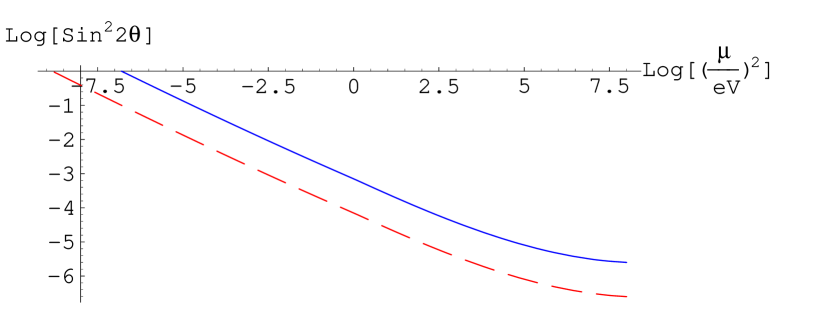
FIG. 1.: The solid and the long dash line are the numerical results which represent the effective degree of freedom equal to 1 and 0.1 respectively. The small dash line separate the equilibrium and out of equilibrium region. The parameter space below the lines are the allowed region.

We note that the bounds derived in both ways i.e. out of equilibrium condition and Boltzman equation are very similar.

In Fig. 2, we give the contributions of individual modes to the total energy density as a function of the mode number for $sin^{2}2\theta=10^{-4}$ and for a range of values for $R^{-1}\equiv\mu$ from $10^{-6}$ eV to $10^{4}$ eV in increasing steps of $10^{2}$ eV. The total contribution is the integral over each line for a given $\mu$.

FIG. 2.: The various lines denote the contribution of the individual modes to the total energy density as a function of the KK mode number for various values of inverse size (in eV) of the extra dimension. The right-most curve corresponds to $\mu=10^{-6}$ eV and for each successive curve, $\mu$ goes up by a factor of 100.

V Conclusion

In this paper, we have studied the constraints of big bang nucleosynthesis on the models with one large extra dimensions and a single bulk neutrino. We find that these bounds allow a range of radius of extra dimension and mixing of bulk to active neutrinos that is of interest for studying solar neutrino oscillations[8]. Our results complement the work of Abazajian, Fuller and Patel[11] who have derived bounds for the case four, five and six extra dimensions. We find it intriguing that the bounds obtained from the naive and crude “out of equilibrium” conditions (given in Eq. (14)) are so similar to the ones obtained from more detailed considerations based on the density matrix equations.

Appendix A

In this appendix, we give details of the out of equilibrium condition used in section II to get the bounds on $\mu^{2}$ and mixing $\theta$. Let us first recall that the out of equilibrium condition is given by:

$$\frac{sin^{2}2\theta}{k^{2}(1+z)^{2}}sin^{2}\frac{\mu^{2}k^{2}}{24T^{6}G^{2}_{F}}\leq 2.5\sqrt{g^{*}}T^{-3}10^{-10}$$ (45)

where all masses are in GeV units and

$$z=\frac{2.15\times 10^{-7}T^{6}}{k^{2}\mu^{2}}\equiv\frac{\alpha}{k^{2}}$$ (46)

Putting in the numerical value of $M_{pl}$ and $G_{F}$ we get

$$\frac{sin^{2}2\theta}{(k+\frac{\alpha}{k})^{2}}sin^{2}(\frac{66.07}{\alpha}k^{2})\leq 2.5\sqrt{g^{*}}T^{-3}10^{-10}$$ (47)

This condition must be satisfied for all $k$ and within our temperature window of an MeV to one GeV. For $\theta,\mu,T$ fixed, if the inequality is satisfied when the expression in the left hand side is a maximum, clearly it is then always satisfied. The $k$ dependent part is given by

$$\frac{sin^{2}(\frac{66.07}{\alpha}k^{2})}{(k+\frac{\alpha}{k})^{2}}=\frac{sin^{2}(66.07y)}{\alpha y(1+\frac{1}{y})^{2}}$$ (48)

$$y\equiv\frac{k^{2}}{\alpha}$$ (49)

Here $\alpha$ is independent on $k$. In this expression, $sin^{2}(66.07y)$ oscillates so fast that in calculating the maximum, we can set $sin^{2}(66.07y)=1$ and finding the maximum of $\frac{1}{y(1+\frac{1}{y})^{2}}$. The maximum is found at $y=1$. $y=1$ implies $k=\sqrt{\alpha}$. Because $k$ must be positive integer, we should choose $k$ equal to the closest integer of $\sqrt{\alpha}$ if $\alpha\geq 1$. For $\alpha<1$, since $y\geq 1$c and it is easy to see that the maximum occurs at the minimum of y, $k=1$ is the maximum point. It is worth noting that, the condition have to be satisfied within a range of temperature (and so a continuous range of $\alpha$).Although at some temperature with a well chosen $\mu$, the constraint can be weaker than those we use, small range of temperature of MeV will cover the period of $sin^{2}(66.07y)$. So the constraint will be that obtained just by setting $sin^{2}(66.07y)=1$.

Now we discuss the two different cases separately.
(i) For $\alpha\geq 1\Rightarrow T\geq(\frac{\mu^{2}}{2.15\times 10^{-7}})^{\frac{1}{6}}\equiv T_{1}$.we have constraint

$$\mu^{2}~{}sin^{2}2\theta\leq 2.15(\frac{T}{GeV})^{3}\sqrt{g^{*}}10^{2}eV^{2}$$ (50)

(ii) For $\alpha<1\Rightarrow T<(\frac{\mu^{2}}{2.15\times 10^{-7}})^{\frac{1}{6}}$. We have constraint

$$sin^{2}2\theta\leq 2.5(1+\alpha)^{2}(\frac{T}{GeV})^{-3}\sqrt{g^{*}}10^{-10}\simeq 2.5(\frac{T}{GeV})^{-3}\sqrt{g^{*}}10^{-10}$$ (51)

In case 2, we have approximate $\alpha\ll 1$. Without making this approximation, the result will give approximately a factor of 2 to $sin^{2}2\theta$. Under this approximation, three different situation appear. they are (i) $T_{1}<MeV\Rightarrow\mu^{2}<2.15\times 10^{-7}eV^{2}$ ,(ii) $MeV<T_{1}<GeV\Rightarrow 2.15\times 10^{-7}eV^{2}<\mu^{2}<2.15\times 10^{11}$ eV²,(iii) $T_{1}\geq GeV\Rightarrow\mu^{2}\geq 2.15\times 10^{11}$ eV².
(i) $T_{1}<MeV$

We have to use eq.(50) with $T=1MeV$ and $g=10.75$. This will give

$$\mu^{2}sin^{2}2\theta<7.07\times 10^{-7}eV^{2}$$ (52)

(ii)$MeV<T_{1}<GeV$

We have to use eq.(50) for T $\in(T_{1},GeV)$ and use eq.(51) for T $\in(MeV,T_{1})$ with $T=T_{1}$ for both cases. This gives respectively

$$\mu~{}sin^{2}2\theta<2.322\times 10^{-3}eV$$ (53)

and

$$\mu~{}sin^{2}2\theta<5.804\times 10^{-4}eV$$ (54)

It is easy to see that even without the approximation that $\alpha\leq 1$, the second equation can go up as high as $1.78\times 10^{-3}eV$ when $T_{1}>1.2MeV$. It is still more stringent than the first.We use the second equation with $\sqrt{g}=5$. This will at most give another factor $(1.5)^{\pm}$ which depend on $\mu$.
(iii)$T_{1}\geq GeV$

Use eq.(51) with $T=1GeV$ and gives

$$sin^{2}2\theta<1.96453\times 10^{-9}$$ (55)

Note that we have omitted the change of the $\delta m^{2}$ due to the matter effect which will only increase the $\delta m^{2}$ as our z is always negative. Increasing $\delta m^{2}$ will increase the frequency the the oscillation term $sin^{2}(66.07y)$ and make it easier to be set to 1.

REFERENCES

- [1] N. Arkani-Hamed, S. Dimopoulos and G. Dvali, Phys. Lett. B429, 263 (1998); Phys. Rev. D59, 086004 (1999); I. Antoniadis, N. Arkani-Hamed, S. Dimopoulos and G. Dvali, Nucl. Phys. B516, 70 (1998).
- [2] C. D. Hoyle, U. Schmidt, B. R. Heckel, E. G. Adelberger, J. Gundlach, D. J. Kapner and H. Swanson, hep-ph/0011014.
- [3] M. Gell-Mann, P. Ramond and R. Slansky, in Supergravity, eds. P. van Niewenhuizen and D.Z. Freedman (North Holland 1979); T. Yanagida, in Proceedings of Workshop on Unified Theory and Baryon number in the Universe, eds. O. Sawada and A. Sugamoto (KEK 1979); R. N. Mohapatra and G. Senjanović, Phys. Rev. Lett. 44, 912 (1980).
- [4] S. Hanestad, astro-ph/0102290; M. J. Fairbarn, hep-ph/0101131; L. Hall and D. Smith, Phys. Rev. D 60, 085008 (1999).
- [5] V. Barger, T. Han, C. Kao and R. J. Zhang, Phys. Lett. B 461, 34 (1999); S. Cullen and M. Perelstein, Phys. Rev. Lett. 83, 268 (1999); C. Hanhardt, J. Pons, D. Phillips and S. Reddy, astro-ph/0102063; G. Raffelt and S. Hannestad, hep-ph/0103201.
- [6] K.R. Dienes, E. Dudas and T. Gherghetta, Nucl. Phys. B557, 25 (1999); N. Arkani-Hamed, S. Dimopoulos, G. Dvali and J. March-Russell, hep-ph/9811448.
- [7] R. N. Mohapatra, S. Nandi and A. Perez-Lorenzana, Phys. Lett. B466, 115 (1999); R. N. Mohapatra and A. Perez-Lorenzana, Nucl. Phys. B 576, 466 (2000).
- [8] D. O. Caldwell, R. N. Mohapatra and S. Yellin, Phys. Rev. Lett. 87, 041601 (2001); Phys. Rev. D 64 073001 (2001).
- [9] A. Farragi and M. Pospelov, Phys. Lett. B 458, 237 (1999); G. Dvali and A.Yu. Smirnov, Nucl. Phys. B563, 63 (1999). A. Ionissian and A. Pilaftsis, hep-ph/9907522; C. S. Lam and J. N. Ng, hep-ph/0104129; G. Mcglaughlin and J. N. Ng, Phys. Lett. B 470, 157 (1999); N. Cosme et al. Phys. Rev. D 63, 113018 (2001); A. Nicolidis and D. T. papadamou, hep-ph/0109048; C. S. Lam, hep-ph/0110142; For a review, see C. S. Lam, hep-ph/0108198.
- [10] R. Barbieri, P. Creminelli and A. Strumia, Nucl. Phys. B 585, 28 (2000).
- [11] K. Abazajian, G. M. Fuller, and M. Patel, hep-ph/0011048.
- [12] A. Lukas, P. Ramond, A. Romanino and G. Ross, Phys. Lett. B 495, 136 (2000);
- [13] K. Olive, G. Steigman and T. Walker, Phys. Rep. 333, 389 (2000); S. Sarkar, Rep. Prog. Phys. 59, 1493 (1996).
- [14] For recent review and references, see A. Dolgov, hep-ph/0109155; D. Kirilova and M. Chizov, astro-ph/0108341.
- [15] D. Fargion and M. Shepkin, Phys. Lett. 146B, 46 (1994).
- [16] D. Notzold and G. Raffelt, Nucl. Phys. B 307, 924 (1988).
- [17] S.Dodelson and L.M. Widrow, Phys. Rev. Lett. 72, 17 (1984).
- [18] P. Langacker, S. Petcov, G. Steigman and S. Toshev, Nucl. Phys. B 282, 589 (1987); R. Barbieri and A. Dolgov, Phys. Lett. B 237, 440 (1990); K. Enquist, K. Kainulainen and J. Maalampi, Phys. Lett. B 244, 186 (1990); ibid B 249, 531 (1990); J. Cline, Phys. Rev. Lett. 68, 3137 (1992); D. P. Kirilova and M. Chizov, Phys. Rev. D 58, 073004 (1998).
- [19] R.Foot,and R.R.Volkas, Phys. Rev. D 55,5147 (1997).