Pomeron effective intercept,
logarithmic derivatives of $F_{2}(x,Q^{2})$
in DIS and Regge models.

P. Desgrolard ^a,, A. Lengyel ^b,, E. Martynov ^c,

^a Institut de Physique Nucléaire de Lyon, IN2P3-CNRS et Université Claude Bernard, 43 boulevard du 11 novembre 1918, F-69622 Villeurbanne Cedex, France

^b Institute of Electron Physics, National Academy of Sciences of Ukraine, 88015 Uzhgorod-015, Universitetska 21, Ukraine

^c Bogoliubov Institute for Theoretical Physics, National Academy of Sciences of Ukraine, 03143 Kiev-143, Metrologicheskaja 14b, Ukraine

Abstract The drastic rise of the proton structure function $F_{2}(x,Q^{2})$ when the Björken variable $x$ decreases, seen at HERA for a large span of $Q^{2}$, may be damped when $x\to 0$ and $Q^{2}$ increases beyond $\sim$ several hundreds GeV². This phenomenon observed in the Regge type models is discussed in terms of the effective Pomeron intercept and of the derivative $B_{x}=\partial{\ell nF_{2}(x,Q^{2})}/\partial{\ell n(1/x)}$. The method of the overlapping bins is used to extract the derivatives $B_{x}$ and $B_{Q}=\partial{\ell nF_{2}(x,Q^{2})}/\partial{Q^{2}}$ from the data on $F_{2}$ for $6.0\cdot 10^{-5}\leq x\leq 0.61$ and $1.2\leq Q^{2}$ ( GeV²) $\leq 5000$. It is shown that the extracted derivatives are well described by recent Regge models with the Pomeron intercept equal one.

1 Introduction

The so-called ”HERA effect” discovered quite long ago by the experimentalists in deep inelastic scattering (DIS) and anticipated by theoreticians has arisen a great interest. It concerns the strong rise of the proton structure functions (SF) $F_{2}(x,Q^{2})$ when the Björken variable $x$ decreases, for the experimentally investigated $Q^{2}$, negative values for the 4-momentum transfer.

This phenomenon is described usually within assumption about power-like behavior of SF at small x

$$F_{2}\ \propto x^{-\lambda}\qquad\mbox{where}\quad\lambda>0.$$ (1)

It is assumed as a rule that the power $\lambda$ is related with the intercept of the Reggeon contribution dominating at $x\to 0$, namely with the Pomeron intercept

$$\lambda=\alpha_{\cal P}(0)-1.$$ (2)

One can find a justification of this treatment in pQCD where the well known BFKL Pomeron in the LL approximation has

$$\lambda_{BFKL}=3N_{c}(\alpha_{s}/\pi)\ell n2\approx 0.4.$$ (3)

However it is necessary to have in mind two circumstances. Firstly, the next-to-leading correction to $\lambda_{BFKL}$ is negative and quite large [1]. Generally, the BFKL Pomeron is only a perturbative approximation to the true Pomeron of which exact properties as well as properties of the whole perturbative series are unknown. Secondly. a power-like $x$-dependence of $F_{2}$ with $\lambda=const>0$ leads to the violation of unitarity providing the Froissart-Martin [2] bound for total cross-section is valid for $\gamma^{*}p$ interaction at least at $x\to 0$. These facts make a ground for a widely accepted opinion that the BFKL Pomeron is to be transformed into a $j$-singularity with intercept exactly equaled to one when all corrections are taken into account . If that is true a power-like behavior of SF at small-$x$ will be changed for a logarithmic-like one (similarly to hadron amplitudes, when a procedure of unitarization or eikonalization is applied). Evidently, such an evolution should lead to a damping of the fast growth of SF at $x\to 0$. We think it is an interesting and important task to investigate the available data to see if they exhibit such a tendency which can be named as damping of the HERA effect.

The detailed analysis [3] of experimental data shows an evident dependence of $\lambda$ on $Q^{2}$. This property of $\lambda$ contradicts relation (2) provided the Pomeron is the universal object as it is observed in pure hadronic reactions [4, 5]. The Pomeron trajectory and hence its intercept must be independent of the external interacting particles, the true universal Pomeron intercept $\alpha_{\cal P}(0)\leq 1$ does not depend on $x$ or $Q^{2}$. It means that a simplified power-like parameterization (1) (with a constant $\lambda>0$) of the forward $\gamma^{*}p$ amplitude or structure function should be considered only as an effective one and can be applied only in narrow intervals of $x$ and $Q^{2}$.

Following the suggestion of [6] the logarithmic $x-$derivative of the structure function (let note it as $B_{x}(x,Q^{2})$ and name it as $x$-slope for brevity)

$$B_{x}(x,Q^{2})={\partial\ell nF_{2}(x,Q^{2})\over\partial\ell n(1/x))}.$$ (4)

was recently extracted [7, 8] from the data on $F_{2}(x,Q^{2})$. However the wrong relation between $x-$slope and ”Pomeron effective intercept” was used in the report [7]. Starting from the structure function written in the form

$$F_{2}(x,Q^{2})=G(Q^{2})\left({1\over x}\right)^{\lambda(x,Q^{2})}$$ (5)

one can define the Pomeron effective intercept as follows

$$\alpha_{\cal P}(x,Q^{2})\equiv 1+\lambda(x,Q^{2}).$$ (6)

”Experimental” data on effective intercept have been extracted in [7] from the data on structure function $F_{2}(x,Q^{2})$ using the relation

$$\lambda(x,Q^{2})={\partial\ell nF_{2}(x,Q^{2})\over\partial\ell n(1/x)}\quad(=\ B_{x}(x,Q^{2})).$$ (7)

The correct equation relating $x$-slope, $B_{x}$, and $\lambda(x,Q^{2})$ must be read however as follows

$${\partial\ell nF_{2}(x,Q^{2})\over\partial\ell n(1/x)}=\lambda(x,Q^{2})+{\partial\lambda(x,Q^{2})\over\partial\ell n(1/x)}.$$ (8)

The relations (7) and (8) strictly coincide only if $\lambda$ does not depend on $x$. We must note that one of the conclusions made in [7, 8] is that experimental data support an independence of $B_{x}(x^{2},Q^{2})$ at $x<0.01$. Nevertheless, in our opinion one need to be more careful.

Supposing that $B_{x}(x,Q^{2})$ does not depend on $x$ at small $x$ we have the following equation for $\lambda(x,Q^{2})$

$$\lambda^{\prime}(x,Q^{2})+\lambda(x,Q^{2})=\lambda_{c}(Q^{2})$$ (9)

where the ”prime” denotes a derivative with respect to $\ell n(1/x)$. There are two possible solutions of this equation.

-1) $\lambda^{\prime}\neq 0$. In this case

$$\lambda(x,Q^{2})=\lambda_{c}(Q^{2})(1-\ell n(1/x))$$

and $\lambda(x,Q^{2})\to-\infty$ at $x\to 0\$ (if $\lambda_{c}(Q^{2})>0$). Such a behavior seems very unnatural.

-2) $\lambda^{\prime}=0$. In this case

$$\lambda(x,Q^{2})=\lambda_{c}(Q^{2}),$$

i.e. it does not depend on $x$ and hence $\sigma_{tot}^{\gamma p}(W)\propto W^{2\lambda_{c}(0)}$ at $W\to\infty$. If we believe in the Pomeron universality we should rather reject than accept this solution as valid one for arbitrary small $x$.

Thus the conclusion about constant $B_{x}(x,Q^{2})$ is possible due to large enough errors and dispersion of the obtained data on $B_{x}$. In fact, it is more likely that $x$-slope depends weakly on $x$, i.e.

$$\left|{\partial\lambda(x,Q^{2})\over\partial\ell n(1/x)}\right|\ll\lambda(x,Q^{2}).$$

However it is difficult without any model assumptions to determine quantitatively how much the derivative of $\lambda$ is small. As we show in the Section 4, the data on $x$-slope are well described in the models with $\alpha_{P}(x,Q^{2})$ and hence with $\lambda(x,Q^{2})$ depending on $x$.

At the same time it seems possible in principle to derive some conclusions about effective intercept from the behavior of $B_{x}(x,Q^{2})$ at small $x$ and high $Q^{2}$. In particular at fixed (even high) $Q^{2}$ and $x\to 0$ unitarized Regge models predict a decreasing of $x$-slope and hence of $\lambda(x,Q^{2})$ [9]. We discuss this subject in more details in the Section 2.

The data on $x$-slope have been given by H1 Collaboration [7] only in the form of figures and cannot be used yet for quantitative comparison with models predictions. Therefore we have performed our own procedure of extracting the local slopes $B_{x}(x,Q^{2})$ for fixed $Q^{2}$ as well as for fixed $x$ based on the method of so-called ”overlapping bins”. A brief description of the method and results are presented in the Section 3.

In addition to the $x$-slope, we consider another logarithmic derivative of the SF, noted $B_{Q}(x,Q^{2})$, named $Q$-slope and defined by

$$B_{Q}(x,Q^{2})\equiv{\partial F_{2}(x,Q^{2})\over\partial\ell nQ^{2}}.$$ (10)

The merit of this slope is mainly due to its relation with the gluon density at $x\ll 1$. The so-called Caldwell plot [10] was the first presentation of the ZEUS data on $B_{Q}$ as a useful tool to study scaling violation of SF and interrelation between soft and hard physics in DIS. However as repeatedly noted [11, 12, 13, 14, 15], the data shown in the original Caldwell plot are derived from $F_{2}$ when averaging over rather large intervals in $Q^{2}$ and for correlated values of $x$ and $<Q^{2}>$. Taking into account the importance of this quantity, it would be useful to have in a wide region of $x$ and $Q^{2}$ the local rather than averaged values of $B_{Q}(x,Q^{2})$. Using the same method of overlapping bins we extract the local $Q$-slopes not only from the H1-data (it was made in [16]) but also from the ZEUS-data and compare with the predictions of our models. The results are presented in the Section 4.

2 Regge Models for proton structure function

There are many phenomenological models e.g. [9, 12, 17, 18, 19, 20, 21, 22, 23, 24] developed within the Regge approach for $\gamma^{*}p$ scattering and structure functions. Some of them [9, 17, 18, 20, 21] deal with a Pomeron having intercept $\alpha_{P}(0)>1$ and can be considered as input for further unitarization [9, 21, 22]. Other ones are constructed from the beginning as models do not violating the Froissart-Martin bound for total cross-sections. Let remind we support the Pomeron universality meaning that, if the Pomeron contribution in pure hadronic amplitudes satisfies unitarity restrictions, it should have the same feature in $\gamma$-hadron scattering.

We consider here two types of unitarized Pomeron, leading at $s\to\infty$ to $\sigma_{tot}(s)\propto\ell ns$ [12, 23] and to $\sigma_{tot}(s)\propto\ell n^{2}(s)$ [24].

2.1 Soft Dipole Pomeron (SDP) model

Defining the Soft Dipole Pomeron model for DIS [12, 23], we start from the expression relating the transverse cross-section of $\gamma^{*}p$ interaction with the proton structure function $F_{2}$ and the optical theorem for forward scattering amplitude.

$$\sigma_{T}^{\gamma^{*}p}(W^{2},Q^{2})=8\pi\Im mA(W^{2},Q^{2};t=0)={4\pi^{2}\alpha\over Q^{2}(1-x)}(1+4m_{p}^{2}x^{2}/Q^{2})F_{2}(x,Q^{2})\ ;$$ (11)

the longitudinal contribution to the total cross-section, $\sigma_{L}^{\gamma^{*}p}=0$ is assumed.

The forward scattering at $W$ far from the $s$-channel threshold $W_{th}=m_{p}$ is dominated by the Pomeron and the $f$-Reggeon

$$A(W^{2},t=0;Q^{2})=P(W^{2},Q^{2})+f(W^{2},Q^{2}),$$ (12)

with the Reggeon contribution

$$f(W^{2},Q^{2})=iG_{f}(Q^{2})(-iW^{2}/m_{p}^{2})^{\alpha_{f}(0)-1}(1-x)^{B_{f}(Q^{2})}\ ,$$ (13)

where

$$G_{f}(Q^{2})={C_{f}\over\left(1+Q^{2}/Q_{f}^{2}\right)^{D_{f}(Q^{2})}}\ ,$$ (14)

$$D_{f}(Q^{2})=d_{f\infty}+{d_{f0}-d_{f\infty}\over 1+Q^{2}/Q_{fd}^{2}}\ ,$$ (15)

$$B_{f}(Q^{2})=b_{f\infty}+{b_{f0}-b_{f\infty}\over 1+Q^{2}/Q^{2}_{fb}}\ .$$ (16)

For the Pomeron contribution, we take a two-component form where the two Pomerons have an intercept equaled to one: one of both being a simple $j$-pole while the other one is a double $j$-pole.

$$P(W^{2},Q^{2})=P_{1}+P_{2}\ ,$$ (17)

with

$$P_{1} = iG_{1}(Q^{2})\ell n(-iW^{2}/m_{p}^{2})(1-x)^{B_{1}(Q^{2})},$$ (18)

$$P_{2} = iG_{2}(Q^{2})(1-x)^{B_{2}(Q^{2})},$$ (19)

where

$$G_{i}(Q^{2}) = {C_{i}\over\left(1+Q^{2}/Q_{i}^{2}\right)^{D_{i}(Q^{2})}}\ ,\qquad i=1,2,$$ (20)

$$\qquad D_{i}(Q^{2}) = d_{i\infty}+{d_{i0}-d_{i\infty}\over 1+Q^{2}/Q_{id}^{2}}\ ,\qquad i=1,2,$$ (21)

$$B_{i}(Q^{2})=b_{i\infty}+{b_{i0}-b_{i\infty}\over 1+Q^{2}/Q^{2}_{ib}}\ ,\qquad i=1,2.$$ (22)

We would like to comment the above expressions, especially the powers $D_{i}$ and $B_{i}$ varying smoothly between constants when $Q^{2}$ goes from $0$ to $\infty$. In spite of an apparently cumbersome form they are a direct generalization of the exponents $d$ and $b$ appearing in each term of the simplest parametrization of the $\gamma^{*}p$-amplitude

$$G(Q^{2})={C\over(1+Q^{2}/Q_{0}^{2})^{d}}\qquad\mbox{and}\qquad(1-x)^{b}\ .$$

Indeed, a fit to experimental data shows unambiguously that the parameters $d$ and $b$ should depend on $Q^{2}$.

Details of the fit to the data and values of fitted parameters can be found in [12, 23]. Here, we only note that in the region $W>3$ GeV², $0\leq Q^{2}\leq 3000$ GeV² and $x\leq 0.75$ we obtained $\chi^{2}/dof=1.073$, where and in what follows ”$dof$” means ”degree of freedom” = number of experimental points $-$ number of free parameters.

We concentrate on asymptotic behavior of $x$-slope, $B_{x}(x,Q^{2})$. At very small $x$ term $P_{1}$ dominates in (12). Hence at $x\ll 1$

$$\begin{array}[]{lll}B_{x}(x,Q^{2})=\displaystyle{\partial{\ell nF_{2}(x,Q^{2})}\over\partial{\ell n(1/x)}}&\approx&\displaystyle{\partial\ell n(K(x,Q^{2})P_{1})\over\partial\ell n(1/x)}\approx{\partial\ell n\left(\ell n(W^{2}/m_{p}^{2})(1-x)^{B_{1}(Q^{2})}\right)\over\partial\ell n(1/x)}\\ &\approx&\displaystyle{1\over\ell n(W^{2}/m_{p}^{2})}\approx{1\over\ell n(Q^{2}/xm_{p}^{2})}\ ,\end{array}$$ (23)

where

$$K(x,Q^{2})={2\pi(1+4m_{p}^{2}x^{2}/Q^{2})\over\alpha Q^{2}(1-x)}\ .$$

Thus in both cases, at fixed $Q^{2}$ and $x\to 0$ as well as at fixed $x$ and $Q^{2}/m_{p}^{2}\gg 1$ (but provided that $P_{1}$ term dominates), in the SDP model $B_{x}(x,Q^{2})\ll 1$. Furthermore, as we show in Section 4, the available data on $x$-slope and its growth with $Q^{2}$ and $1/x$ are very well described within the model. The decreasing of $B_{x}$ is predicted far out of HERA kinematic region.

2.2 Generalized Logarithmic Pomeron (GLP) model

In [23] we have constructed a model incorporating a slow rise of $\sigma_{tot}^{\gamma p}(W^{2})$ and simultaneously a fast rise of $F_{2}(x,Q^{2})$ at large $Q^{2}$ and small $x$. The model is in a sense intermediate between the above Soft Dipole Pomeron model and the two-Pomeron model [17] of Donnachie and Landshoff . The model is defined as follows.

$$F_{2}(x,Q^{2})=F_{0}+F_{s}+F_{f},$$ (24)

$$F_{0}=C_{0}{Q^{2}\over\left(1+Q^{2}/Q^{2}_{0}\right)^{d_{0}}}(1-x)^{B_{0}(Q^{2})},$$ (25)

$$F_{s}=C_{s}{Q^{2}\over(1+Q^{2}/Q^{2}_{s})^{d_{s}}}L(W^{2},Q^{2})(1-x)^{B_{s}(Q^{2})},$$ (26)

where

$$L(W^{2},Q^{2})=\ell n\left[1+{a\over(1+Q^{2}/Q^{2}_{s\ell})^{d_{s\ell}}}\left({Q^{2}\over xm_{p}^{2}}\right)^{\epsilon}\right]\ ,$$ (27)

$$F_{f}=C_{f}{Q^{2}\over(1+Q^{2}/Q^{2}_{f})^{d_{f}}}\left({Q^{2}\over xm_{p}^{2}}\right)^{\alpha_{f}(0)-1}(1-x)^{B_{f}(Q^{2})}$$ (28)

and

$$B_{i}(Q^{2})=b_{i\infty}+{b_{i0}-b_{i\infty}\over 1+Q^{2}/Q^{2}_{ib}},\qquad i=0,s,f.$$ (29)

For $\gamma p$ total cross-section the model gives

$$\sigma_{tot}^{\gamma p}(W^{2})=4\pi^{2}\alpha\left[C_{0}+C_{s}L(W^{2},0)+C_{f}\left({W^{2}\over m_{p}^{2}}-1\right)^{\alpha_{f}(0)-1}\right]\ ,$$ (30)

with

$$L(W^{2},0)\ =\ \ell n\left(1+a\left({W^{2}\over m_{p}^{2}}-1\right)^{\ \epsilon}\right)\ .$$

A few comments on the above model are needed.

The new logarithmic factor in (26) can be rewritten in the form

$$L(W^{2},Q^{2})=\ell n\left[1+{a\over(1+Q^{2}/Q^{2}_{s\ell})^{d_{s\ell}}}\left({W^{2}+Q^{2}\over m_{p}^{2}}-1\right)^{\epsilon}\right].$$

Consequently, at $Q^{2}=0$, we have $L(W^{2},0)\approx\epsilon\ell n(W^{2}/m_{p}^{2})$ at $W^{2}/m_{p}^{2}\gg 1$. Thus, $\sigma_{tot}^{\gamma p}(W^{2})\propto\ell nW^{2}$ at $W^{2}\gg m_{p}^{2}$. A similar behaviour can be seen at moderate $Q^{2}$ when the denominator is $\sim 1$. However at not very large $W^{2}/m_{p}^{2}$ or at sufficiently high $Q^{2}$ the argument of logarithm is close to 1, and then

$$L(W^{2},Q^{2})\approx{a\over(1+Q^{2}/Q^{2}_{s\ell})^{d_{s\ell}}}\left({W^{2}+Q^{2}\over m_{p}^{2}}-1\right)^{\epsilon}\ ,$$

simulating a Pomeron contribution with intercept $\alpha_{P}(0)=1+\epsilon$.

We are going to justify that, in spite of its appearance, the GLP model cannot be treated as a model with a hard Pomeron, even when $\epsilon$ issued from the fit is not small. In fact, the power $\epsilon$ inside the logarithm is NOT really the intercept (more exactly it is not $\alpha_{P}(0)-1$). Intercept is defined as position of singularity of the amplitude in $j$-plane at $t=0$. It is shown in [23] that in the present GLP model the true leading Regge singularity is located exactly at $j=1$: it is a double pole due to the logarithmic dependence.

Thus this model should be considered rather as a Dipole Pomeron model. In order to distinguish it from the Soft Dipole Pomeron model of Section 2.1, we have named this model ”Generalized Logarithmic Pomeron” (GLP) model. A fit performed [23] has given $\chi^{2}/dof=1.064$. Parameters of the GLP model are presented in [23]; for the power $\epsilon$ we obtained $\epsilon=0.4536\pm 0.0015$. Finally, we can say that the GLP model only mimics a contribution of a hard Pomeron although non incorporating explicitely one. The asymptotic behavior of $x$-slope at fixed $Q^{2}$ and $x\to 0$ in the GLP model coincides with SDP one:

$$B_{x}(x\to 0,Q^{2})\approx{1\over\ell n(Q^{2}/xm_{p}^{2})}\to 0.$$

In an other kinematical limit: $x\ll 1$, but fixed, and $Q^{2}\to\infty$, the GLP model gives a behavior

$$B_{x}(x\ll 1,Q^{2}\to\infty)\approx\epsilon\left(1-\Phi(Q^{2})\left({1\over x}\right)^{\epsilon}\right)\ ,$$ (31)

where

$$\Phi(Q^{2})={a(Q^{2}/m_{p}^{2})^{\epsilon}\over(1+Q^{2}/Q^{2}_{sl})^{d_{sl}}}\propto\left({Q^{2}\over m_{p}^{2}}\right)^{\epsilon-d_{sl}}\to 0\qquad\mbox{at}\qquad Q^{2}\to\infty\ ;$$ (32)

because in accordance with the fit [23] $d_{sl}=0.7016\pm 0.0022$ and hence ($\epsilon$ is given above) $\epsilon-d_{sl}\approx-0.25$.

2.3 Cudell-Soyez Pomeron (CSP) model

Recently an other model obeying unitarity restrictions for Pomeron contribution was suggested in [24] to account for HERA data (i.e. low $x$ structure functions). The model has the form

$$F_{2}(Q^{2}/2\nu,Q^{2})=a(Q^{2})\ell n^{2}\left(\nu/\nu_{0}(Q^{2})\right)+c(Q^{2})+d(Q^{2})(2\nu)^{\alpha_{f}(0)-1}\ ,$$ (33)

where $\nu=Q^{2}/(xm_{p}^{2})$ and leads to

$$\sigma_{tot}^{\gamma p}(s)\propto\ell n^{2}(s)\qquad\mbox{at}\qquad s\to\infty\ .$$ (34)

The explicit form of functions $a(Q^{2}),\nu_{0}(Q^{2}),c(Q^{2})$ and $d(Q^{2})$ can be found in the original paper [24]. This model is particularized by construction to the region of small $x$-SF. We have refitted it to our set of data [23] restricted to $x\leq 0.07$ and $0\leq Q^{2}\leq 3000$ GeV² and obtained $\chi^{2}/dof\approx 1.0$. One can show that at fixed $Q^{2}$ and $x\to 0$ the slope $B_{x}(x,Q^{2})$ calculated in CSP model is exactly twice as large as the slope calculated in SDP model although they practically coincide at the available $x<0.03$ and $Q^{2}<1000$ GeV² (see Section  4).

3 Extraction of the local slope $B_{x}(x,Q^{2})$ from the SF data

As noted in the introduction, the $x$-slope is a precious tool to settle if, either yes or no, a damping of the HERA effect does exist. Actually, we need the sets of experimental data on $B_{x}(x,Q^{2})$ as a function of $x$ at fixed $Q^{2}$ as well as at fixed $x$ versus sufficiently high $Q^{2}$. Unfortunately, because the $x-$slope is not a measurable observable it should be extracted, when possible, from the available data on the SF.

To extract $x$-slopes with a good accuracy we adapt the so-called method of ”overlapping bins” [25], originally intended for analyzing the local nuclear slope of the first diffraction cone in $pp$ and $\bar{p}p$ elastic scattering. Then the method was used to determine averaged $x$-slopes [13] and the local ones [14] before new, more precise and complete, data appeared. Let briefly describe the main idea of the method.

Provided that the SF has been measured for a given $Q^{2}$ at $N$ $x$-points lying in some interval $[x_{min},x_{max}]$, we adopt the following procedure. First, we divide this interval into subintervals or elementary ”bins” (with $n_{b}$ measurements in each of them, assumed for simplicity to be the same for all bins). Once the first bin is chosen, the second bin is obtained from the first one by shifting only one point of measurement (of course one could shift by any number of points less or equal $n_{b}$, the shift of one point we choose is the minimal one giving rise to the maximal number of overlapping bins). The third bin is obtained from the second bin by the shift of one data point etc… . Thus, we define $N-n_{b}+1$ overlapping bins for a given $Q^{2}$. For each ($k$-th) bin, $n_{b}$ must be large enough and its width (in $x$) small enough to allow fitting the SF with the simplest form directly involving the $x$-slope

$$F_{2}(x)=A\left({1\over x}\right)^{B}\ ,\quad(\mbox{for a given fixed}\quad Q^{2})\ .$$ (35)

The parameter $B$ represents the value of the $x$-slope $B\left(<x>_{k},Q^{2}\right)$, ”measured”, at $Q^{2}$ and at the ”weighted average” $<x>_{k}$ defined in the $k$-th bin as (see [26])

$$<x>_{k}=exp\bigg{(}-{\sum{\ln x_{i}\over\Delta y_{i}}\over\sum{1\over\Delta y_{i}}}\bigg{)}\ ,\quad k\in{[1,N-n_{b}+1]}\ ,$$ (36)

where $x_{i}$ is the value of $x$ at which the structure function $y_{i}$ is measured with the uncertainty $\Delta y_{i}$; the summations run over all data points, $i=1,2,...,n_{b}$ of the bin. This yields the ”experimental” values of $B_{x}(x,Q^{2})$ with the corresponding standard errors determined in the fit of (35) to the data. Then the procedure is to be repeated for all bins and ultimately for the other $Q^{2}$’s at which the SF have been measured.

The next step in extracting and analyzing $B_{x}(x,Q^{2})$ is the determination of the slopes at fixed $x$ as function of $Q^{2}$, making use of results of the first step. As a rule, the sets of $<x>_{k}$, at different $Q^{2}$, do not coincide. So in order to get the $x-$slope at fixed $x$ and at different $Q^{2}$ we interpolate (or extrapolate but not far from the $x$-interval under consideration) already extracted $B_{x}$ at the given $Q^{2}$ to the chosen $x$. This has been made simply assuming a linear $x-$dependence of $B_{x}$.

The above method of overlapping bins is applied to the whole available data set. We have separated the data in three groups: ZEUS, H1 and Fixed Target experiments which were analyzed independently each of the others. The resulting values of $B_{x}(x,Q^{2})$ are shown in the Figs. 1 - 3 where they are compared to the predictions of theoretical models. The results of the interpolation for $x=0.005,0.01,0.05$ and 0.08 are presented in the Fig.4.

We would like to comment some ”technical” points in our analysis and results.

• In order to keep its local character to the $x$-slope and to obtain a maximal possible number of ”measurements”, we have given only the case when five points are taken in each elementary bin. We found a weak dependence of the extracted slopes if the number of points in a bin goes from $N=4$ to $N=6$.

• In spite of a high accuracy of the recent data from HERA, the dispersion of the SF-values influences the resulting values of $B_{x}$ and its uncertainty. For some bins, for example, we were unable to fit (35) to the data with $\chi^{2}\leq 1$, so we could not obtain in all cases reasonable errors. Nevertheless we show these extracted values (only with $\chi^{2}\leq 3$) in the figures and use them for interpolation to the $x$ under interest because even with those points the extracted set of data for $B_{x}(x,Q^{2})$ at fixed $x$ is quite poor. Of course, this reduces the reliability of our results, but only slightly because the total number of ”bad” bins remains small.

• ”Experimental” values of $B_{x}$ at fixed $x$ shown in Fig. 4 are obtained by a linear interpolation within the two subsets of local $x$-slopes, extracted from the HERA and from the fixed target measurements of SF.

• One can see in Fig. 4 that some points deviate strongly from the groups constituted by the other ones. This is due to the strong influence of the points (of $F_{2}$ as well as of $B_{x}$) which are at the ends of the $x$-bins and which also ”fall out of a common line” (see also item ii above). To solve this problem, a possible way would be to exclude some of them from the analysis; another way would be to enlarge the number of points in an elementary bin loosing, however, the local character of the extracted $x$-slope. A more detailed analysis of the available data related to more numerous measurements of the primary observable, $F_{2}(x,Q^{2})$ would be necessary to obtain more precise data for $B_{x}(x,Q^{2})$.

• In all figures we show for comparison the recently published data (open circles) on slopes of H1 Collaboration [8]. Our slopes extracted by the method of overlapping bins and those obtained in [8] are in a good agreement.

4 Comparison of the slopes data with the models predictions and conclusions

There are many parameterizations of the proton structure functions which successfully accommodate for the whole - or a part of - available data set and in particular for the steep rise of the SF when $x$ decreases for a large span of $Q^{2}$ values . Several of them have given explicitly some hints (see e.g.  [19, 12, 9, 23, 24]) on the existence of a slowing down of the HERA effect.

Here we concentrate on the three models (SDP, GLP, CSP) considered in the Section 2 satisfying to Pomeron universality, i.e. with Pomeron contribution which is the same for hadron-hadron and $\gamma$-proton elastic interactions. These models lead to $\sigma_{tot}^{\gamma p}(s)\propto\ell n^{\mu}(s)$ at $s\to\infty$ with $\mu=1$ (SDP and GLP models) and with $\mu=2$ as in CSP model.

All models well describe the extracted data on $B_{x}(x,Q^{2})$, particularly a growth of this quantity with available $Q^{2}$ when $x$ is fixed, in spite of the fact that the real Pomeron intercept is constant and equal one.

One can see in the Figs. 1 - 3 and in Fig. 4 that the theoretical curves calculated in all models are closed each to others for small and intermediate $Q^{2}$ while they are noticeably different for high $Q^{2}\mathrel{\hbox to0.0pt{\lower 4.0pt\hbox{\hskip 1.0pt$\sim$}\hss}\raise 1.0pt\hbox{$>$}}200$ GeV². As concerns the CSP model, one must recall that it can be applied in its original form only for small $x$. That is why the data for $x\mathrel{\hbox to0.0pt{\lower 4.0pt\hbox{\hskip 1.0pt$\sim$}\hss}\raise 1.0pt\hbox{$>$}}0.05$ are not described by this model. However, we checked it, it is possible to extend its ability to describe SF in the large-$x$ region modifying each $i$-term of (33) by a factor $(1-x)^{B_{i}(Q^{2})}$. Unhappily, an extra bump-like structure in $B_{x}$ is predicted by such a modified CSP model which is not supported by available data.

It is seen in Fig. 4 that the GLP model predicts the growth of $B_{x}$ at $Q^{2}\to\infty$ to the asymptotic value $B_{as}=\epsilon\approx 0.454$. A decreasing of $x$-slope predicted in the SDP and CSP models is observed at such high values of $1/x$ and $Q^{2}$ that it is problematic to detect the phenomenon in future experiments. However it seems possible to distinguish SDP and CSP models from GLP one when the data at fixed $x$ and higher $Q^{2}$ will be known.

Returning to the often assumed constancy of $B_{x}$ at $x<0.01$, we would like to note that the 3 considered models exhibit a very weak $x$-dependence of $B_{x}$ at small $x$. At the same time $B_{x}(x\to 0,Q^{2})\to 0$ for any fixed $Q^{2}$.

The method of overlapping bins has been applied also in order to extract from the SF data the other derivative, the $Q-$slope. Again as for the $x$-slope, we extracted $B_{Q}$ separately from the H1, ZEUS and Fixed Target data. The results as well as the theoretical curves calculated in the models under interest are presented in Fig. 5 and Fig. 6. The Caldwell-plot with the corresponding points and curves for SDP (solid line), GLP (short dotted line) and CSP (long dotted line) models is presented in Fig. 7. One can see that all models are in good agreement with the data. However they predict quite different behaviors outside the region of available data, in particular at small $x$ and high $Q^{2}$ (see Fig. 5).

Our short conclusion is the following. We have shown that the available data on the proton structure function as well as on the $x$- and $Q$-slopes are well described in the Regge models that realize the idea of a universal Pomeron. Pomeron singularity in these models is the same in hadron-hadron and in photon-hadron elastic forward amplitudes. It is located in angular momentum plane at $j=1$ not violating the unitarity restrictions. These models predict a decreasing of $x$-slope and $\lambda(x,Q^{2})$ for fixed $Q^{2}$ and $x\to 0$.

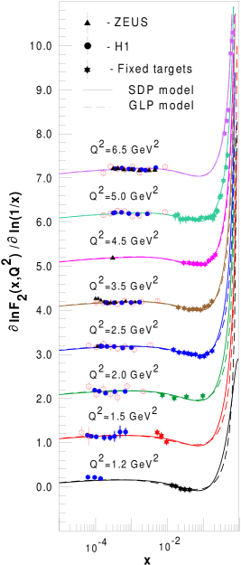
Figure 1: $B_{x}(x,Q^{2})$ as function of $x$ at small $Q^{2}$. The open circles are the data from [8]. The other notations are given in the figure

Figure 2: The same as in Fig. 1 but for intermediate $Q^{2}$.

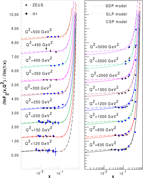
Figure 3: The same as in Fig. 1 but for high values of $Q^{2}$.

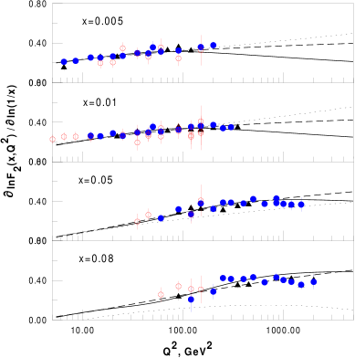
Figure 4: $B_{x}(x,Q^{2})$ at fixed $x$ versus $Q^{2}$. The notations for experimental points and theoretical curves are the same as in Figs. 1-3. Only data of [8] closed to the given values of $x$ are shown.

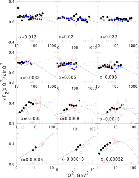
Figure 5: Comparison of $Q$-slopes (10) at fixed $x$ versus $Q^{2}$ extracted by the overlapping bins method from ZEUS (full triangles) and H1 (full circles) $F_{2}$-data with the $Q$-slopes of [8] (open circles) and with the predictions of SDP (solid lines) and GLP (dashed lines) models.

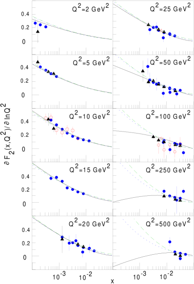
Figure 6: Same as in Fig. 5 but at fixed $Q^{2}$ versus $x$.

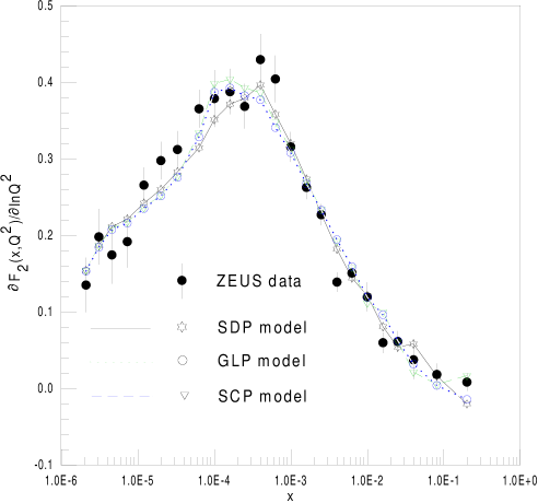
Figure 7: The $B_{Q}$-slope at the selected ZEUS points given by the solid circles (Caldwell plot). $B_{Q}$ calculated in SDP, GLP and CSP models are presented also.

References

- [1] V.S. Fadin, L.N. Lipatov, Phys. Lett. B 429, 127 (1998) and references therein.
- [2] M. Froissart, Phys. Rev. 123, 1053 (1961); A. Martin, Nuovo Cim. 42, 930 (1966).
- [3] J. Breitweg et al. , ZEUS Collaboration, Eur. Phys. J. C 7, 609 (1999); see also [8].
- [4] J.R. Cudell et al. , Phys. Rev. D 61, 034019 (2000).
- [5] J.R. Cudell et al. , hep-ph/0107226 (2001).
- [6] H. Navelet, R. Peschanski, S. Wallon, Mod. Phys. Lett. A 9, 3393 (1994).
-
[7]
H1 Collaboration, available at
www-h1.desy.de/h1/www/publications/conf/conf_list.html - [8] C. Adloff et al. , H1 Collaboration, DESY-01-104, hep-ex/0108035 (2001).
- [9] S.M. Troshin, N.E. Tyurin, Europhys. Lett. 37, 238 (1997); hep-ph/0102322 (2001).
- [10] A. Caldwell, DESY Theory Workshop, DESY, Hamburg (Germany), October 1997; see also [3].
- [11] E. Gotsman, E. Levin, U. Maor, Nucl. Phys. B 425, 369 (1998); Nucl. Phys. B 539, 535 (1999).
- [12] P. Desgrolard, A. Lengyel, E. Martynov, Eur. Phys. Jour. C 7, 655 (1999).
- [13] P. Desgrolard, L. Jenkovszky, A. Lengyel, F. Paccanoni, Phys. Lett. B 459, 265 (1999).
- [14] P. Desgrolard, A. Lengyel, E. Martynov, Nucl. Phys. (Proc. Supp.) B 99, 168 (2001); hep-ph/0009313 (2000).
- [15] A.B. Kaidalov, C. Merino, D. Petermann, Eur. Phys. J. C 20, 301 (2001).
- [16] H1 Collaboration, Preprint DESY00-181 (2000); hep-ph/0012053.
- [17] A. Donnachie, P.V. Landshoff, Zeit. Phys. C 61, 139 (1994); Phys. Lett. B 437, 408 (1998); Phys. Lett. B 518, 63, (2001).
- [18] H. Abramovicz, E.Levin, A. Levy, U. Maor, Phys. Lett. B 269, 465 (1991); H. Abramovicz, A. Levy, DESY 97-251, hep-ph/9712415 (1997).
- [19] M. Bertini et al. , in ”Strong interactions at long distances”, edited by L. Jenkovszky, Hadronic Press, Palm Harbor, FL U.S.A, 1995), p.181.
-
[20]
A. Capella, A. Kaidalov, C. Merino, J. Tran Thanh Van, Phys. Lett. B
337, 358 (1994),
A. Kaidalov, C. Merino, D. Pertermann, Eur. Phys. J C 20, 301 (2001). - [21] V.A. Petrov, A.V. Prokudin, Proceedings of the VIII Blois Workshop, International Conference on Elastic and Diffractive Scattering, edited by V.A. Petrov and A.V. Prokudin (Protvino, Russia, 28 June - 2 July, 1999), p. 95; hep-ph/9912248 (1999).
- [22] A. Capella, E.G. Ferreiro, C.A. Salgado, A.B. Kaidalov, Nucl. Phys. B 593, 336 (2001).
- [23] P. Desgrolard, E. Martynov, Preprint LYCEN2001-35, hep-ph/0105277 (2001).
- [24] J.R. Cudell, G. Soyez, Phys. Lett. B 516, 77 (2001).
- [25] J. Kontros, A. I. Lengyel, in Strong Interaction at long distances, edited by L. Jenkovszky (Hadronic Press, Palm Harbor, FL USA, 1995), p.67.
- [26] ZEUS collaboration, J. Breitweg et al. , Eur. Phys. J. C 7, 609 (1999).