hep-ph/02xxx

Rare decay $B\rightarrow X_{s}l^{+}l^{-}$ in a CP spontaneously broken two Higgs doublet model

Chao-Shang Huang ^a, Wei Liao ^b, Qi-shu Yan ^c and Shou-hua Zhu^d

^a Institute of Theoretical Physics, Academia Sinica,
P.O.Box 2735, Beijing 100080, P.R.China
^b The Abdus Salam International Centre for Theoretical Physics,
P.O.Box 586, 34014 Trieste, Italy
^c Institute of High Energy Physics, Chinese Academy of Sciences,
P.O.Box 918-4, Beijing 100039, P. R. China
^d Institut für Theoretische Physik, Universität Karlsruhe,
D-76128 Karlsruhe, Germany

The Higgs boson mass spectrum and couplings of neutral Higgs bosons to fermions are worked out in a CP spontaneously broken two Higgs doublet model in the large tan$\beta$ case. The differential branching ratio, forward-backward asymmetry, CP asymmetry and lepton polarization for $B\rightarrow X_{s}l^{+}l^{-}$ are computed. It is shown that effects of neutral Higgs bosons are quite significant when $\tan\beta$ is large. Especially, the CP violating normal polarization $P_{N}$ can be as large as several percents.

PACS number(s): 12.60.-i 12.60.Fr 13.20.-v

I Introduction

The recent results on CP violation in $B_{d}$ - $\bar{B}_{d}$ mixing have been reported by the BaBar and Belle Collaborations [1], which can be explained in the Standard Model (SM) within theoretical and experimental uncertainties. As it is well-known, the direct CP violation measurement, Re($\epsilon^{\prime}$/$\epsilon$), in the Kaon system [2] can also be accommodated by the CKM phase in the SM within the theoretical uncertainties. However, the CKM phase is not enough to explain the matter-antimatter asymmetry in the universe and gives the contribution to electric dipole moments (EDMs) of electron and neutron much smaller than the experimental limits of EDMs of electron and neutron. Therefore, one needs new sources of CP violation, which has been one of motivations to search new theoretical models beyond the SM.

The minimal extension of the SM is to enlarge the Higgs sector [3]. It has been shown that if one adheres to the natural flavor conservation (NFC) in the Higgs sector, then a minimum of three Higgs doublets are necessary in order to have spontaneous CP violation [4]. However, the constraint can be evaded if one gives up NFC. If NFC is broken, one can obtain a so-called general or model III two-Higgs-doublet model (2HDM) in which the CP symmetry is explicitly broken. In this paper, however, we will discuss a simpler 2HDM in which the Higgs potential is CP invariant and $Z_{2}$ symmetry softly broken. Comparing with the model I or model II 2HDM, the Higgs potential of this model has an additional linear term of Re($\phi^{+}_{1}\phi_{2}$) and different self couplings for the real and image parts of $\phi_{1}^{+}\phi_{2}$ [5, 6, 7]. In this model (we call it model IV 2HDM hereafter) CP symmetry can be spontaneously broken [5, 6, 7]. So the model IV is the minimal among the extensions of the SM that provide a new source of CP violation. It should be noted that, in addition to the above terms, if one adds a linear term of Im($\phi^{+}_{1}\phi_{2}$), then one will obtain a CP softly broken 2HDM [7].

Flavor changing neutral current (FCNC) transitions $B\rightarrow X_{s}\gamma$ and $B\rightarrow X_{s}l^{+}l^{-}$ provide testing grounds for the SM at the loop level and sensitivity to new physics. Rare decays $B\rightarrow X_{s}l^{+}l^{-}(l=e,\mu)$ have been extensively investigated in both SM and the beyond [8, 9]. In these processes contributions from exchanging neutral Higgs bosons (NHB) can be safely neglected because of smallness of $\frac{m_{l}}{m_{W}}(l=e,\mu)$ if tan$\beta$ is smaller than about 25. The inclusive decay $B\rightarrow X_{s}\tau^{+}\tau^{-}$ has also been investigated in the SM, the model II 2HDM and SUSY models with and without including the contributions of NHB [10, 11, 12, 13, 14, 15, 16, 17, 18, 19], in a CP softly broken 2HDM [5], as well as in the technicolor model with scalars [20]. In this paper we extend to investigate $B\rightarrow X_{s}l^{+}l^{-}(l=e,\mu,\tau)$ with emphasis on CP violation effects in model IV. Although there is little difference between the CP softly and spontaneously broken models [7], the mass spectrum and consequently some phenomenological effects are different.

The paper is organized as follows. In section 2, we describe the details of the model IV and work out the Higgs mass spectrum and couplings of Higgs bosons to fermions. Section 3 is devoted to the effective Hamiltonian responsible for $B\rightarrow X_{s}l^{+}l^{-}$. We calculate Wilson coefficients and give all the leading terms. In Section 4 the formula for CP violating observables and lepton polarizations in $B\rightarrow X_{s}l^{+}l^{-}$ are given. We give the numerical results in section 5. Finally, in section 6 we draw conclusions and discussions.

II The CP spontaneously broken 2HDM

For two complex $y=1$, $SU(2)_{w}$ doublet scalar fields, $\phi_{1}$ and $\phi_{2}$, the simplest Higgs potential, which is NFC softly broken, can be written as [7]:

$$V(\phi_{1},\phi_{2}) = \sum_{i=1,2}[m_{i}^{2}\phi_{i}^{+}\phi_{i}+\lambda_{i}(\phi_{i}^{+}\phi_{i})^{2}]+m_{3}^{2}Re(\phi_{1}^{+}\phi_{2})+m_{4}^{2}Im(\phi_{1}^{+}\phi_{2})$$ (2)

$$+\lambda_{3}[(\phi_{1}^{+}\phi_{1})(\phi_{2}^{+}\phi_{2})]+\lambda_{4}[\mbox{Re}(\phi_{1}^{+}\phi_{2})]^{2}+\lambda_{5}[\mbox{Im}(\phi_{1}^{+}\phi_{2})]^{2}$$

Hermiticity requires that all parameters are real. It should be noted that the potential is CP softly broken due to the presence of the term $m_{4}^{2}Im(\phi_{1}^{+}\phi_{2})$. We assume that the minimum of the potential is at

$$<\phi_{1}>=\left(\begin{array}[]{c}0\\ v_{1}\end{array}\right),\ \ \ \ <\phi_{2}>=\left(\begin{array}[]{c}0\\ v_{2}e^{i\xi}\end{array}\right),$$ (7)

which breaks $SU(2)\times U(1)$ down to $U(1)_{EM}$ and simultaneously the CP invariance. The requirement that the vacuum is at least a stationary point of the potential results in the following three constraints:

$$sin2\xi v_{1}v_{2}(\lambda_{4}-\lambda_{5})+sin\xi m^{2}_{3}-cos\xi m_{4}^{2}=0,$$ (8)

$$v_{2}cos\xi[2C_{2}+v_{1}^{2}(\lambda_{4}-\lambda_{5})]+v_{1}m_{3}^{2}=0,$$ (9)

$$sin\xi(v_{1}^{2}C_{1}-v_{2}^{2}C_{2})-v_{1}v_{2}m_{4}^{2}=0,$$ (10)

where

$$C_{1}=m_{1}^{2}+2\lambda_{1}v_{1}^{2}+(\lambda_{3}+\frac{\lambda_{4}+\lambda_{5}}{2})v_{2}^{2},$$ (11)

$$C_{2}=m_{2}^{2}+2\lambda_{2}v_{2}^{2}+(\lambda_{3}+\frac{\lambda_{4}+\lambda_{5}}{2})v_{1}^{2}.$$ (12)

For the CP classically invariant case (model IV), $m_{4}^{2}$=0, eq.(10) reduces to

$$m_{1}^{2} = -[2\lambda_{1}v_{1}^{2}+(\lambda_{3}+\lambda_{5})v_{2}^{2}],$$ (13)

$$m_{2}^{2} = -[2\lambda_{2}v_{2}^{2}+(\lambda_{3}+\lambda_{5})v_{1}^{2}],$$ (14)

$$m_{3}^{2} = -2v_{1}v_{2}(\lambda_{4}-\lambda_{5})\cos\xi.$$ (15)

¿From eq. (15), one can see that the necessary condition to have spontaneously broken CP is $\lambda_{4}\neq\lambda_{5}$ and $m_{3}^{2}\neq 0$, i.e., the real and image parts of $\phi_{1}^{+}\phi_{2}$ have different self-couplings and there exists a linear term of Re($\phi^{+}_{1}\phi_{2}$) in the potential.

We can write the potential at the stationary point as:

$$V = m_{1}^{2}v_{1}^{2}+m_{2}^{2}v_{2}^{2}+\lambda_{1}v_{1}^{4}+\lambda_{2}v_{2}^{4}+(\lambda_{3}+\lambda_{5})v_{1}^{2}v_{2}^{2}$$ (17)

$$+(\lambda_{4}-\lambda_{5})v_{1}^{2}v_{2}^{2}\left[(\cos\xi-\Delta)^{2}-\Delta^{2}\right],$$

with

$$\Delta=-\frac{m_{3}^{2}}{2v_{1}v_{2}(\lambda_{4}-\lambda_{5})}.$$

One can see that in order for the spontaneous CP-breaking to occur with $\sin\xi\neq 0$, the following inequalities must hold:

$$\lambda_{4}-\lambda_{5}>0,\\ -1<\Delta<1,$$

and the potential minimum is at $\cos\xi=\Delta$, which is automatically satisfied due to Eq. (15).

In the following we will work out the mass spectrum of the Higgs bosons in model IV. For charged components, the mass-squared matrix for negative states is

$$-\lambda_{5}\left(\begin{array}[]{cc}v_{1}^{2}&-v_{1}v_{2}e^{i\xi}\\ -v_{1}v_{2}e^{-i\xi}&v_{2}^{2}\end{array}\right),$$ (20)

Diagonalizing the mass-squared matrix results in one zero-mass Goldstone state:

$$G^{-}=e^{i\xi}\sin\beta\phi_{2}^{-}+\cos\beta\phi_{1}^{-},$$ (21)

and one massive charged Higgs boson state:

$$H^{-} = e^{i\xi}\cos\beta\phi_{2}^{-}-\sin\beta\phi_{1}^{-},$$ (22)

$$m_{H^{-}} = |\lambda_{5}|v^{2},$$ (23)

where $tan\beta=v_{2}/v_{1}$ and $v^{2}=v_{1}^{2}+v_{2}^{2}$, which is determined by $2m_{W}^{2}/g^{2}$. Correspondingly we could also get the positive states $G^{+}$ and $H^{+}$.

For neutral Higgs components, because CP-conservation is broken, the mass-squared matrix is $4\times 4$, which can not be simply separated into two $2\times 2$ matrices as usual. After rotating the would-be Goldestone boson $(v_{1}{\rm Im}\phi_{1}^{0}+v_{2}{\rm Im}\phi_{2}^{0})/v$ away, the elements of the mass matrix of the three physical neutral Higgs bosons $\mu_{ij}$, in the basis of {${\rm Re}\phi_{1}^{0},{\rm Re}\phi_{2}^{0},(v_{2}{\rm Im}\phi_{1}^{0}-v_{1}{\rm Im}\phi_{2}^{0})/v$}, can be written as

$$\mu_{11} = 4\lambda_{1}v_{1}^{2}+(\lambda_{4}-\lambda_{5})v_{2}^{2}c^{2}_{\xi}$$ (24)

$$\mu_{12} = v_{1}v_{2}[2\lambda_{3}+\lambda_{4}c^{2}_{\xi}+\lambda_{5}(1+s^{2}_{\xi})]$$ (25)

$$\mu_{13} = \frac{1}{2}(\lambda_{4}-\lambda_{5})v_{2}vs_{2\xi}$$ (26)

$$\mu_{22} = 4\lambda_{2}v_{2}^{2}+(\lambda_{4}-\lambda_{5})v_{1}^{2}c^{2}_{\xi}$$ (27)

$$\mu_{23} = \frac{1}{2}(\lambda_{4}-\lambda_{5})s_{2\xi}v_{1}v$$ (28)

$$\mu_{33} = (\lambda_{4}-\lambda_{5})v^{2}s^{2}_{\xi}$$ (29)

where $s,c$ represent $\sin,\cos$. In eq. (29), the constraints in eq. (15) have been used. In the case of large $\tan\beta$ which is what we are interested in , if we neglect all terms proportional to $v_{1}$, i.e., if the parameters $\lambda_{i}$’s are of the same order, one can get from above mass matrix that one of the Higgs boson masses is zero, which is obviously in conflict with current experiments. Therefore, in stead we shall discuss the cases in which there is a hierarchy of order of magnitude between the parameters, $\lambda_{1}\gg$ other $\lambda$’s, and other terms proportional to $v_{1}$ in eq. $(\ref{e3})$ are negligible. For simplicity, we define $\bar{\lambda}=\lambda_{4}-\lambda_{5}$ and $\tilde{\lambda}=4\lambda_{1}v_{1}^{2}$. Diagonalizing the Higgs boson mass-squared matrix results in

$$\left(\begin{array}[]{c}H^{0}_{1}\\ H^{0}_{2}\\ H^{0}_{3}\end{array}\right)=\sqrt{2}\left(\begin{array}[]{ccc}c_{\alpha}&s_{\alpha}&0\\ -s_{\alpha}&c_{\alpha}&0\\ 0&0&1\end{array}\right)\left(\begin{array}[]{c}{\rm Im}\phi_{1}^{0}\\ {\rm Re}\phi_{1}^{0}\\ {\rm Re}\phi_{2}^{0}\end{array}\right)$$ (39)

with masses

$$m_{H^{0}_{1},H^{0}_{2}}^{2} = \frac{1}{2}\left(\mu_{11}+\mu_{33}\mp\sqrt{(\mu_{11}-\mu_{33})^{2}+4\mu_{13}^{2}}\right)$$ (40)

and the mixing angle

$$\tan(2\alpha) = \frac{2\mu_{13}}{\mu_{33}-\mu_{11}}.$$ (41)

In model IV, it is assumed that the fermions obtain masses in the same way as in model II 2HDM. That is, the up-type quarks get masses from Yukawa couplings to the Higgs doublet $\phi_{2}$ and down-type quarks and leptons get masses from Yukawa couplings to the Higgs doublet $\phi_{1}$. Then it is straightforward to obtain the couplings of neutral Higgs bosons to fermions

$$H^{0}_{1}\bar{f}f:\ \ \ \ -\frac{igm_{f}}{2m_{w}c_{\beta}}(s_{\alpha}+ic_{\alpha}\gamma_{5})$$ (42)

$$H^{0}_{2}\bar{f}f:\ \ \ \ -\frac{igm_{f}}{2m_{w}c_{\beta}}(c_{\alpha}-is_{\alpha}\gamma_{5})$$ (43)

where $f$ represents down-type quarks and leptons. The coupling of $H_{3}^{0}$ to f is not enhanced by tan$\beta$ and will not be given here explicitly. The couplings of the charged Higgs bosons to fermions are the same as those in the CP-conservative 2HDM (model II, see Ref. [22]). This is in contrary with the model III [23] in which the couplings of the charged Higgs to fermions can be quite different from model II. It is easy to see from Eqs. (43) that the contributions come from exchanging NHB is proportional to $\sqrt{2}G_{F}s_{\alpha}c_{\alpha}m_{f}^{2}/\cos^{2}\beta$, so that the constraint due to EDM translate into the constraint on $\sin 2\alpha\tan^{2}\beta$ ($1/\cos\beta\sim\tan\beta$ in the large $\tan\beta$ limit). According to the analysis in Ref. [24], we have the constraint

$$\sqrt{|\sin 2\alpha|}\tan\beta<50$$ (44)

from the neutron EDM. And the constraint from the electron EDM is not stronger than Eq. (44). It is obvious from Eq. (44) that there is a constraint on $\alpha$ only if $\tan\beta>50$.

III The effective Hamiltonian for $B\rightarrow X_{s}l^{+}l^{-}$

As it is well-known, inclusive decay rates of heavy hadrons can be calculated in heavy quark effective theory (HQET) [25] and it has been shown that the leading terms in $1/m_{Q}$ expansion turn out to be the decay of a free (heavy) quark and corrections stem from the order $1/m_{Q}^{2}$ [26]. In what follows we shall calculate the leading term. The effective Hamiltonian describing the flavor changing processes $b\rightarrow sl^{+}l^{-}$ can be defined as

$$H_{eff}=\frac{4G_{F}}{\sqrt{2}}V_{tb}V^{*}_{ts}(\sum_{i=1}^{10}C_{i}(\mu)O_{i}(\mu)+\sum_{i=1}^{10}C_{Q_{i}}(\mu)Q_{i}(\mu))$$ (45)

where $O_{i}(i=1,\cdots,10)$ is the same as that given in the ref.[8], $Q_{i}$’s come from exchanging the neutral Higgs bosons and are defined in Ref. [12]. The explicit expressions of the operators governing $B\rightarrow X_{s}l^{+}l^{-}$ are given as follows:

$$O_{7} = (e/16\pi^{2})m_{b}(\bar{s}_{L\alpha}\sigma^{\mu\nu}b_{R\alpha})F_{\mu\nu},$$ (46)

$$O_{8} = (e/16\pi^{2})(\bar{s}_{L\alpha}\gamma^{\mu}b_{L\alpha})\bar{l}\gamma_{\mu}l,$$ (47)

$$O_{9} = (e/16\pi^{2})(\bar{s}_{L\alpha}\gamma^{\mu}b_{L\alpha})\bar{l}\gamma_{\mu}\gamma_{5}l,$$ (48)

$$Q_{1} = (e^{2}/16\pi^{2})(\bar{s}_{L\alpha}b_{R\alpha})(\bar{l}l),$$ (49)

$$Q_{2} = (e^{2}/16\pi^{2})(\bar{s}_{L\alpha}b_{R\alpha})(\bar{l}\gamma_{5}l).$$ (50)

For the large $\tan\beta$ case, we can generally write the couplings as following:

$$HH^{\pm}G^{\mp} : \ \ \ \ \pm igC_{HH^{+}G^{-}},$$ (51)

$$HH^{\pm}W^{\mp} : \ \ \ \ igC_{HH^{+}W^{-}},$$ (52)

$$H\bar{b}b : \ \ \ \ igm_{b}\tan\beta(C_{b}+\bar{C}_{b}\gamma_{5}),$$ (53)

$$H\bar{l}l : \ \ \ \ igm_{l}\tan\beta(C_{l}+\bar{C}_{l}\gamma_{5}).$$ (54)

In model VI, we obtain

$$C_{H_{1}H^{+}G^{-}} = -\sqrt{2}ve^{i\xi}\left[c_{\alpha}(\lambda_{4}s_{\xi}+i\lambda_{5}c_{\xi})+s_{\alpha}(\lambda_{4}c_{\xi}-i\lambda_{5}s_{\xi}+\tilde{\lambda})\right],$$ (55)

$$C_{H_{2}H^{+}G^{-}} = -\sqrt{2}ve^{i\xi}\left[-s_{\alpha}(\lambda_{4}s_{\xi}+i\lambda_{5}c_{\xi})+c_{\alpha}(\lambda_{4}c_{\xi}-i\lambda_{5}s_{\xi}+\tilde{\lambda})\right],$$ (56)

$$C_{H_{1}H^{+}W^{-}} = -\frac{s_{\alpha}+ic_{\alpha}}{2},$$ (57)

$$C_{H_{2}H^{+}W^{-}} = -\frac{c_{\alpha}-is_{\alpha}}{2}.$$ (58)

and $C_{b},C_{l},\bar{C}_{b},\bar{C}_{l}$ can be extracted from Eq. (43).

At the renormalization point $\mu=m_{W}$ the coefficients $C_{i}$’s in the effective Hamiltonian have been given in the ref.[8] and $C_{Q_{i}}$’s are (neglecting the $O(tg\beta)$ term)

$$C_{Q_{1}}(m_{W}) = \frac{m_{b}m_{l}tg^{2}\beta x_{t}}{sin^{2}\theta_{W}}\{\frac{1}{m_{H}^{2}}\left[-m_{W}^{2}(C_{b}+\bar{C}_{b})f_{1}+C_{HH^{+}G^{-}}f_{2}-m_{W}C_{HH^{+}W^{-}}f_{2}\right]C_{l}-\frac{f_{3}}{4m_{W}^{2}}\},$$ (59)

$$C_{Q_{2}}(m_{W}) = \frac{m_{b}m_{l}tg^{2}\beta x_{t}}{sin^{2}\theta_{W}}\{\frac{1}{m_{H}^{2}}\left[-m_{W}^{2}(C_{b}+\bar{C}_{b})f_{1}+C_{HH^{+}G^{-}}f_{2}-m_{W}C_{HH^{+}W^{-}}f_{2}\right]\bar{C}_{l}+\frac{f_{3}}{4m_{W}^{2}}\},$$ (60)

$$C_{Q_{3}}(m_{W}) = \frac{m_{b}e^{2}}{m_{l}g_{s}^{2}}(C_{Q_{1}}(m_{W})+C_{Q_{2}}(m_{W})),$$ (61)

$$C_{Q_{4}}(m_{W}) = \frac{m_{b}e^{2}}{m_{l}g_{s}^{2}}(C_{Q_{1}}(m_{W})-C_{Q_{2}}(m_{W})),$$ (62)

$$C_{Q_{i}}(m_{W}) = 0,~{}~{}~{}~{}i=5,\cdots,10$$ (63)

where

$$f_{1} = \frac{x_{t}lnx_{t}}{x_{t}-1}-\frac{x_{H^{\pm}}lnx_{H^{\pm}}-x_{t}lnx_{t}}{x_{H^{\pm}}-x_{t}},$$ (64)

$$f_{2} = \frac{x_{t}lnx_{t}}{(x_{t}-1)(x_{H^{\pm}}-x_{t})}-\frac{x_{H^{\pm}}lnx_{H^{\pm}}}{(x_{H^{\pm}}-x_{t})(x_{H^{\pm}}-1)},$$ (65)

$$f_{3} = \frac{1}{x_{H^{\pm}}-x_{t}}(\frac{lnx_{t}}{x_{t}-1}-\frac{lnx_{H^{\pm}}}{x_{H^{\pm}}-1})$$ (66)

with $x_{i}=m_{i}^{2}/m_{w}^{2}$. It would be instructive to note that in addition to the diagrams of exchanging neutral Higgs bosons, the box diagram with a charged Higgs and a W in the loop also gives a leading contribution proportional to $\tan^{2}\beta$ [27, 28].

Neglecting the strange quark mass, the effective Hamiltonian (45) leads to the following matrix element for $b\rightarrow sl^{+}l^{-}$

$$M = \frac{G_{F}\alpha}{\sqrt{2}\pi}V_{tb}V^{*}_{ts}[C^{eff}_{8}\bar{s}_{L}\gamma_{\mu}b_{L}\bar{l}\gamma^{\mu}l+C_{9}\bar{s}_{L}\gamma_{\mu}b_{L}\bar{l}\gamma^{\mu}\gamma^{5}l$$ (67)

$$+ 2C_{7}m_{b}\bar{s}_{L}i\sigma^{\mu\nu}\frac{q^{\nu}}{q^{2}}b_{R}\bar{l}\gamma^{\mu}l+C_{Q_{1}}\bar{s}_{L}b_{R}\bar{l}l+C_{Q_{2}}\bar{s}_{L}b_{R}\bar{l}\gamma^{5}l],$$ (68)

where [8, 10, 29]

$$C^{eff}_{8} = C_{8}+\{g(\frac{m_{c}}{m_{b}},\hat{s})$$ (69)

$$+ \frac{3}{\alpha^{2}}k\sum_{V_{i}=J/\psi,\psi^{\prime},\psi^{\prime\prime}...}\frac{\pi M_{V_{i}}\Gamma(V_{i}\rightarrow l^{+}l^{-})}{M^{2}_{V_{i}}-q^{2}-iM_{V_{i}}\Gamma_{V_{i}}}\}(3C_{1}+C_{2}),$$ (70)

with $\hat{s}=q^{2}/m_{b}^{2},~{}~{}q=(p_{\mu^{+}}+p_{\mu^{-}})^{2}$. In (69) $g(\frac{m_{c}}{m_{b}},\hat{s})$ arises from the one-loop matrix element of the four-quark operators and can be found in Refs. [8, 30]. The second term in the brace in (69) estimates the long-distance contribution from the intermediates, J/$\psi$, $\psi^{\prime}$, $\psi^{\prime\prime}$ … [8, 29]. For l=$\tau$, the lowest resonance J/$\psi$ in the $c\bar{c}$ system does not contribute because the invariant mass square of the lepton pair is $s>4m_{\tau}^{2}$. In our numerical calculations, we choose $k(3C_{1}+C_{2})=-0.875$ [31].

The QCD corrections to coefficients $C_{i}$ and $C_{Q_{i}}$ can be incooperated in the standard way by using the renormalization group equations. Although the $C_{i}$ at the scale $\mu=O(m_{b})$ have been given in the next-to-leading order approximation (NLO) without including mixing with $Q_{i}$ [32], we use the values of $C_{i}$ only in the leading order approximation (LO) since no $C_{Q_{i}}$ have been calculated in NLO. The $C_{i}$ and $C_{Q_{i}}$ with LO QCD corrections at the scale $\mu=O(m_{b})$ have been given in Ref. [12]:

$$C_{7}(m_{b}) = \eta^{-16/23}\left[C_{7}(m_{W})-[\frac{58}{135}(\eta^{10/23}-1)+\frac{29}{189}(\eta^{28/23}-1)]C_{2}(m_{W})\right.$$ (72)

$$\left.-0.012C_{Q_{3}}(m_{W})\right],$$

$$C_{8}(m_{b}) = C_{8}(m_{W})+\frac{4\pi}{\alpha_{s}(m_{W})}[-\frac{4}{33}(1-\eta^{-11/23})+\frac{8}{87}(1-\eta^{-29/23})]C_{2}(m_{W}),$$ (73)

$$C_{9}(m_{b}) = C_{9}(m_{W}),$$ (74)

$$C_{Q_{i}}(m_{b}) = \eta^{-\gamma_{Q}/\beta_{0}}C_{Q_{i}}(m_{W}),~{}~{}i=1,2,$$ (75)

where $\gamma_{Q}=-4$ [33] is the anomalous dimension of $\bar{s}_{L}b_{R}$, $\beta_{0}=11-2n_{f}/3$, and $\eta=\alpha_{s}(m_{b})/\alpha_{s}(m_{W})$.

After a straightforward calculation, we obtain the invariant dilepton mass distribution [12]

$$\frac{{\rm d}\Gamma(B\rightarrow X_{s}l^{+}l^{-})}{{\rm d}s} = B(B\rightarrow X_{c}l{\bar{\nu}})\frac{{\alpha}^{2}}{4\pi^{2}f(m_{c}/m_{b})}(1-s)^{2}(1-\frac{4t^{2}}{s})^{1/2}\frac{|V_{tb}V_{ts}^{*}|^{2}}{|V_{cb}|^{2}}D(s)$$ (76)

$$D(s) = |C_{8}^{eff}|^{2}(1+\frac{2t^{2}}{s})(1+2s)+4|C_{7}|^{2}(1+\frac{2t^{2}}{s})(1+\frac{2}{s})$$ (79)

$$+|C_{9}|^{2}[(1+2s)+\frac{2t^{2}}{s}(1-4s)]+12{\rm Re}(C_{7}C_{8}^{eff*})(1+\frac{2t^{2}}{s})$$

$$+\frac{3}{2}|C_{Q_{1}}|^{2}(s-4t^{2})+\frac{3}{2}|C_{Q_{2}}|^{2}s+6{\rm Re}(C_{9}C_{Q_{2}}^{*})t$$

where s=$q^{2}/m_{b}^{2}$, t=$m_{l}/m_{b}$, $B(B\rightarrow X_{c}l{\bar{\nu}})$ is the branching ratio of $B\rightarrow X_{c}l{\bar{\nu}}$, $f$ is the phase-space factor and f(x)=$1-8x^{2}+8x^{6}-x^{8}-24x^{4}\ln~{}x$.

We also give the forward-backward asymmetry

$$A(s)=\frac{\int^{1}_{0}dz\frac{d^{2}\Gamma}{dsdz}-\int^{0}_{-1}dz\frac{d^{2}\Gamma}{dsdz}}{\int^{1}_{0}dz\frac{d^{2}\Gamma}{dsdz}+\int^{0}_{-1}dz\frac{d^{2}\Gamma}{dsdz}}=-3\sqrt{\frac{1-4t^{2}}{s}}\frac{E(s)}{D(s)}$$ (80)

where $z=\cos\theta$ and $\theta$ is the angle between the momentum of the B-meson and that of $l^{+}$ in the center of mass frame of the dileptons $l^{+}l^{-}$. Here,

$$E(s)={\rm Re}(C_{8}^{eff}C_{9}^{*}s+2C_{7}C_{9}^{*}+C_{8}^{eff}C_{Q1}^{*}t+2C_{7}C_{Q2}^{*}t).$$ (81)

IV CP violating observables and lepton polarizations in $B\rightarrow X_{s}l^{+}l^{-}$

The formulas for CP violating observables and lepton polarizations in $B\rightarrow X_{s}l^{+}l^{-}$ have been given in our previous paper [5]. We give the formula below in order to make the paper self-contained. The CP asymmetry for the $B\rightarrow X_{s}l^{+}l^{-}$ and $\overline{B}\rightarrow\overline{X}_{s}l^{+}l^{-}$ is commonly defined as

$$A_{CP}(s)=\frac{{\rm d}\Gamma/{\rm d}s-{\rm d}\overline{\Gamma}/{\rm d}s}{{\rm d}\Gamma/{\rm d}s+{\rm d}\overline{\Gamma}/{\rm d}s}.$$ (82)

The CP asymmetry in the forward-backward asymmetry for $B\rightarrow X_{s}l^{+}l^{-}$ and $\overline{B}\rightarrow\overline{X}_{s}l^{+}l^{-}$ is defined as

$$B_{CP}(s)=A(s)-\overline{A}(s)$$ (83)

It is easy to see from Eq. (79) that the CP asymmetry $A_{CP}$, in general, is very small because the weak phase difference in $C_{7}C_{8}^{eff}$ arises from the small mixing of $O_{7}$ with $Q_{3}$ (see Eq. (72)). In contrast to $A_{CP}$, $B_{CP}$ can reach a large value when $\tan\beta$ is large, as can be seen from Eqs. (81) and (63). Therefore, we propose to measure $B_{CP}$ in order to search for new CP violation sources.

Let us now discuss the lepton polarization effects. We define three orthogonal unit vectors:

$$\vec{e}_{L} = \frac{\vec{p}_{1}}{\left|\vec{p}_{1}\right|}~{},$$ (84)

$$\vec{e}_{N} = \frac{\vec{p}_{s}\times\vec{p}_{1}}{\left|\vec{p}_{s}\times\vec{p}_{1}\right|}~{},$$ (85)

$$\vec{e}_{T} = \vec{e}_{N}\times\vec{e}_{L}~{},$$ (86)

where $\vec{p}_{1}$ and $\vec{p}_{s}$ are the three momenta of the $\ell^{-}$ lepton and the $s$ quark, respectively, in the center of mass of the $\ell^{+}~{}\ell^{-}$ system. The differential decay rate for any given spin direction $\vec{n}$ of the $\ell^{-}$ lepton, where $\vec{n}$ is a unit vector in the $\ell^{-}$ lepton rest frame, can be written as

$$\frac{d\Gamma\left(\vec{n}\right)}{{\rm d}s}=\frac{1}{2}\left(\frac{d\Gamma}{{\rm d}s}\right)_{\!\!\!0}\Big{[}1+\left(P_{L}\,\vec{e}_{L}+P_{N}\,\vec{e}_{N}+P_{T}\,\vec{e}_{T}\right)\cdot\vec{n}\Big{]}~{},$$ (87)

where the subscript ”0” corresponds to the unpolarized case, and $P_{L},~{}P_{T}$, and $P_{N}$, which correspond to the longitudinal, transverse and normal projections of the lepton spin, respectively, are functions of $s$. ¿From Eq. (87), one has

$$P_{i}(s)=\frac{{\displaystyle{\frac{d\Gamma}{ds}\left(\vec{n}=\vec{e}_{i}\right)-\frac{d\Gamma}{ds}\left(\vec{n}=-\vec{e}_{i}\right)}}}{{\displaystyle{\frac{d\Gamma}{ds}\left(\vec{n}=\vec{e}_{i}\right)+\frac{d\Gamma}{ds}\left(\vec{n}=-\vec{e}_{i}\right)}}}~{}.$$ (88)

The calculations for the $P_{i}$’s (i = $L,~{}T,~{}N$) lead to the following results:

$$P_{L} = (1-\frac{4t^{2}}{s})^{1/2}\frac{D_{L}(s)}{D(s)},$$ (89)

$$P_{N} = \frac{3\pi}{4s^{1/2}}(1-\frac{4t^{2}}{s})^{1/2}\frac{D_{N}(s)}{D(s)},$$ (90)

$$P_{T} = -\frac{3\pi t}{2s^{1/2}}\frac{D_{T}(s)}{D(s)},$$ (91)

where

$$D_{L}(s) = {\rm Re}\left(2(1+2s)C_{8}^{eff}C_{9}^{*}+12C_{7}C_{9}^{*}-6tC_{Q_{1}}C_{9}^{*}-3sC_{Q_{1}}C_{Q_{2}}^{*}\right),$$ (92)

$$D_{N}(s) = {\rm Im}\left(2sC_{Q_{1}}C_{7}^{*}+sC_{Q_{1}}C_{8}^{eff*}+sC_{Q_{2}}C_{9}^{*}+4tC_{9}C_{7}^{*}+2tsC_{8}^{eff\ *}C_{9}\right),$$ (93)

$$D_{T}(s) = {\rm Re}\left(-2C_{7}C_{9}^{*}+4C_{8}^{eff}C_{7}^{*}+\frac{4}{s}|C_{7}|^{2}-C_{8}^{eff}C_{9}^{*}\right.$$ (95)

$$\left.+s|C_{8}^{eff}|^{2}-\frac{s-4t^{2}}{2t}C_{Q_{1}}C_{9}^{*}-\frac{s}{t}C_{Q_{2}}C_{7}^{*}-\frac{s}{2t}C_{8}^{eff}C_{Q_{2}}^{*}\right).$$

$P_{i}$ (i=L, T, N) have been given in the ref.  [15], where there are some errors in $P_{T}$ and they gave only two terms in $D_{N}$, the numerator of $P_{N}$. We remind that $P_{N}$ is the CP-violating projection of the lepton spin onto the normal of the decay plane. Because $P_{N}$ in $B\rightarrow X_{s}l^{+}l^{-}$ comes from both the quark and lepton sectors, purely hadronic and leptonic CP-violating observables, such as $d_{n}$ or $d_{e}$, do not necessarily strongly constrain $P_{N}$ [34]. So it is advantageous to use $P_{N}$ to investigate CP violation effects in some extensions of SM [35]. In the model IV, as pointed out above, $d_{n}$ and $d_{e}$ constrain $\sqrt{|\sin 2\alpha|}\tan\beta$ and consequently $P_{N}$ through $C_{Q_{i}}$ ($i=1,2$) (see Eq. (95)).

V Numerical results

The following parameters have been used in the numerical calculations:

$$m_{t,{\rm pole}}=175Gev,~{}m_{b,{\rm pole}}=5.0Gev,~{}m_{c,,{\rm pole}}=1.3Gev,$$

$$~{}m_{\mu}=0.105Gev,~{}m_{\tau}=1.777Gev,~{}\eta=1.67.$$

Without losing generality, we assume $0<\xi<2\pi$. For Higgs masses, as an example, we choose $m_{H^{\pm}}=250Gev$ (see discussions below), the lightest neutral Higgs mass fixed to 100 $Gev$, and the heavier neutral Higgs mass being 500 $Gev$. It should be pointed out that the region of $\xi$ will be constrained due to this specific choice of neutral Higgs boson masses ( see eq. (40)), which is the reason why there are gaps in Fig. 1 and Figs. 4-10. For l=e, the contributions of neutral Higgs bosons are negligible due to smallness of the electron mass so that results are almost the same as those in SM. So we only give numerical results for l=$\mu,\tau$. We shall analyse the constraint from $b\rightarrow s\gamma$ in the first subsection and give the numerical results for l=$\tau,\mu$ in the second and third subsections respectively.

A The constraint from $b\rightarrow s\gamma$

Because the couplings of the charged Higgs to fermions in Model IV are the same as those in the model II, the constraint on $\tan\beta$ due to effects arising from the charged Higgs are the same as those in the model II. The constraint on $tg\beta$ from $K-\bar{K}$ and $B-\bar{B}$ mixing, $\Gamma(b\rightarrow s\gamma)$,$\Gamma(b\rightarrow c\tau\bar{\nu}_{\tau})$ and $R_{b}$ has been given [36]

$$0.7\leq tg\beta\leq 0.52(\frac{m_{H^{\pm}}}{1Gev})$$ (96)

(and the lower limit $m_{H^{\pm}}\geq 200Gev$ has also been given in the ref. [36]). In Ref. [37], it is pointed out that lower bound of the charged Higgs is about 250 GeV if one adopts conservative approach to evaluate the theoretical uncertainty; on the other hand, adding different theoretical errors in quadrature leads to $m_{H^{\pm}}>370$ GeV. Indeed, these bounds are quite sensitive to the errors of the theoretical predictions and to the details of the calculations.

Due to the mixing of $O_{7}$ with $Q_{3}$, $C_{7}(\mu)$ is dependent of $C_{Q_{3}}$ (see eq. (30) ). So we have to see if the experimental results of $b\rightarrow s\gamma$ impose a constraint on our model parameters (see Ref. [38] for the detail discussion of the constraint on $C_{7}$). From the equation [39, 40]

$$\frac{Br(B\to X_{s}\gamma)}{Br(B\to X_{c}e\bar{\nu}_{e})}=\frac{|V_{ts}^{*}V_{tb}|^{2}}{|V_{cb}|^{2}}\frac{6\alpha}{\pi f(z)}|C^{\rm eff}_{7}(\mu_{b})|^{2}$$ (97)

and the experimental results for $b\rightarrow s\gamma$ [41]

$$2.0\times 10^{-4}<Br(b\rightarrow s\gamma)<4.5\times 10^{-4},$$ (98)

we can get the constraint on $|C_{7}|$. In fig. 1, we show the $C_{7}$ as a function of $\xi$. One can see from the figure that even for $\tan\beta=50$, the model can still escape the experimental constraint.

B $B\rightarrow X_{s}\tau^{+}\tau^{-}$

Numerical results for $B\rightarrow X_{s}\tau^{+}\tau^{-}$ are shown in Figs. 2-7. From Figs. 2 and 3, we can see that the contributions of NHBs to the differential branching ratio $d\Gamma/ds$ and forward-backward asymmetry $A_{s}$ are significant when $\tan\beta$ is 50 and the masses of NHBs are in the reasonable region, which is similar to the case of model II 2HDM without CP violation [12].

Figs. 4 and 5 are devoted to $B_{CP}$ and $P_{N}$ as a function of $\xi$. From Fig. 4, one can see that $B_{CP}$ can reach about $1.5\%$ for the favorable parameters, and depends strongly on $\xi$. Fig. 5 shows that $P_{N}$ depends also strongly on $\xi$ and can be as large as $8\%$. It should be noted that experimentally the observables after integrating $s$ are more accessible than those for specific s, therefore we present also the integrated-$P_{N}$ ( the integration range of s is 0.6-1 which is apart from the resonance region ) in Fig. 5 and Fig. 8. Our numerical results [(b) in Fig. 5] show that the shape of the integrated-$P_{N}$, which can also reach several percent, is similar to that for specific s. For the illumination purpose, we shall present the results for specific s in most of figures.

Figs. 6 and 7 show the longitudinal and transverse polarizations respectively. It is obvious that the contributions of NHBs can change the polarizations greatly, especially when $\tan\beta$ is large. The longitudinal polarization of $B\rightarrow X_{s}l^{+}l^{-}$ has been calculated in SM and several new physics scenarios [10]. Switching off the NHB contributions, our results are in agreement with those in Ref. [10].

C $B\rightarrow X_{s}\mu^{+}\mu^{-}$

Because the contributions of NHBs to the differential branching ratio, forward-backward asymmetry and $B_{CP}$ for the process $B\rightarrow X_{s}\mu^{+}\mu^{-}$ are so small if even $tan\beta$ is as large as 100, which is due to the strong suppression ( $\propto m_{l}^{2}/m_{w}^{2}$ ), we do not show the results here. However, for the lepton polarizations, the suppression is proportional to $m_{l}/m_{w}$, which is not so strong, and consequently NHBs can make relatively significant contributions. We show the numerical result of $P_{N}$ and integrated-$P_{N}$ in Fig. 8, $P_{L}$ and $P_{T}$ in Figs. 9 and 10.

Fig. 8 shows that $P_{N}$ is sensitive to $\xi$ and can reach several percent when $\tan\beta=50$. For $\tan\beta$=10, $P_{N}$ is unobservablly small. From Fig. 9-10, one can see that the contributions of NHBs can change the longitudinal and transverse polarizations greatly, especially when $\tan\beta$ is large.

VI Conclusions and discussions

In summary, we have calculated the differential branching ratio, back-forward asymmetry, lepton polarizations and some CP violated observables for $B\rightarrow X_{s}l^{+}l^{-}$ in the model IV 2HDM. As the main features of the model, NHBs play an important role in inducing CP violation, in particular, for large $\tan\beta$. We propose to measure $B_{CP}$ (defined in section IV) instead of the usual CP asymmetry $A_{CP}$, because the former could be observed for l=$\tau$ if $\tan\beta$ is large enough and the latter is too small to be observed. The CP violating normal polarization $P_{N}$ can reach several percents for l=$\tau$ and $\mu$ when tan$\beta$ is large and Higgs boson masses are in the reasonable range, which could be observed in the future B factories with $10^{8}$- $10^{12}$ B hadrons per year [42]. It should be noted that the results are sensitive to the mass of the charged Higgs boson. If the charged Higgs boson is heavy (say $>400$ GeV), the effects arising from new physics would disappear. If we take the mass of charged Higgs boson to be 200 Gev which is the lowest limit allowed by $B\rightarrow X_{s}\gamma$, the CP violation effects will be more significant than those given in the paper. Comparing the results in the paper with those in the CP softly broken 2HDM, the main difference is the different $\xi$-dependence. Therefore, it is possible to discriminate the model IV from the other 2HDMs by measuring the CP-violated observables such as $B_{CP}$, $P_{N}$ if the nature chooses large $\tan\beta$ and a light charged Higgs boson. Otherwise, it is difficult to discriminate them.

FIG. 1.: $C_{7}$ as a function of $\xi$ with $m_{H^{\pm}}=250GeV$, and solid and dashed lines represent $\tan\beta=50$ and $10$, dot-dashed line represents the case of switching off $C_{Q_{i}}$ contributions. The region between two straight solid lines is permitted by the $b\rightarrow s\gamma$ experiment.

FIG. 2.: Differential branching ratio as function of $s$ for $B\rightarrow X_{s}\tau^{+}\tau^{-}$, where $\xi=\pi/3$, solid and dashed lines represent $\tan\beta=50$ and $10$, dot-dashed line represents the case of switching off $C_{Q_{i}}$ contributions.

FIG. 3.: Forward-backward asymmetry as function of $s$, other captions are same as Fig. 2.

FIG. 4.: $B_{CP}$ as function of $\xi$, for $B\rightarrow X_{s}\tau^{+}\tau^{-}$, where $s=0.8$, solid and dashed lines represent $\tan\beta=50$ and $10$.

FIG. 5.: $P_{N}$ (a) and integrated-$P_{N}$ (b) as functions of $\xi$ for $B\rightarrow X_{s}\tau^{+}\tau^{-}$, where $s=0.8$ for (a), solid and dashed lines represent $\tan\beta=50$ and $10$, dot-dashed line represents the case of switching off $C_{Q_{i}}$ contributions.

FIG. 6.: $P_{L}$ as function of $\xi$, other captions are same as Fig. 5 (a).

FIG. 7.: $P_{T}$ as function of $\xi$, other captions are same as Fig. 5 (a).

FIG. 8.: $P_{N}$ (a) and integrated-$P_{N}$ (b) as functions of $\xi$ for $B\rightarrow X_{s}\mu^{+}\mu^{-}$, where $s=0.6$ for (a), solid and dashed lines represent $\tan\beta=50$ and $10$, dot-dashed line represents the case of switching off $C_{Q_{i}}$ contributions.

FIG. 9.: $P_{L}$ as function of $\xi$, other captions are same as Fig. 8 (a).

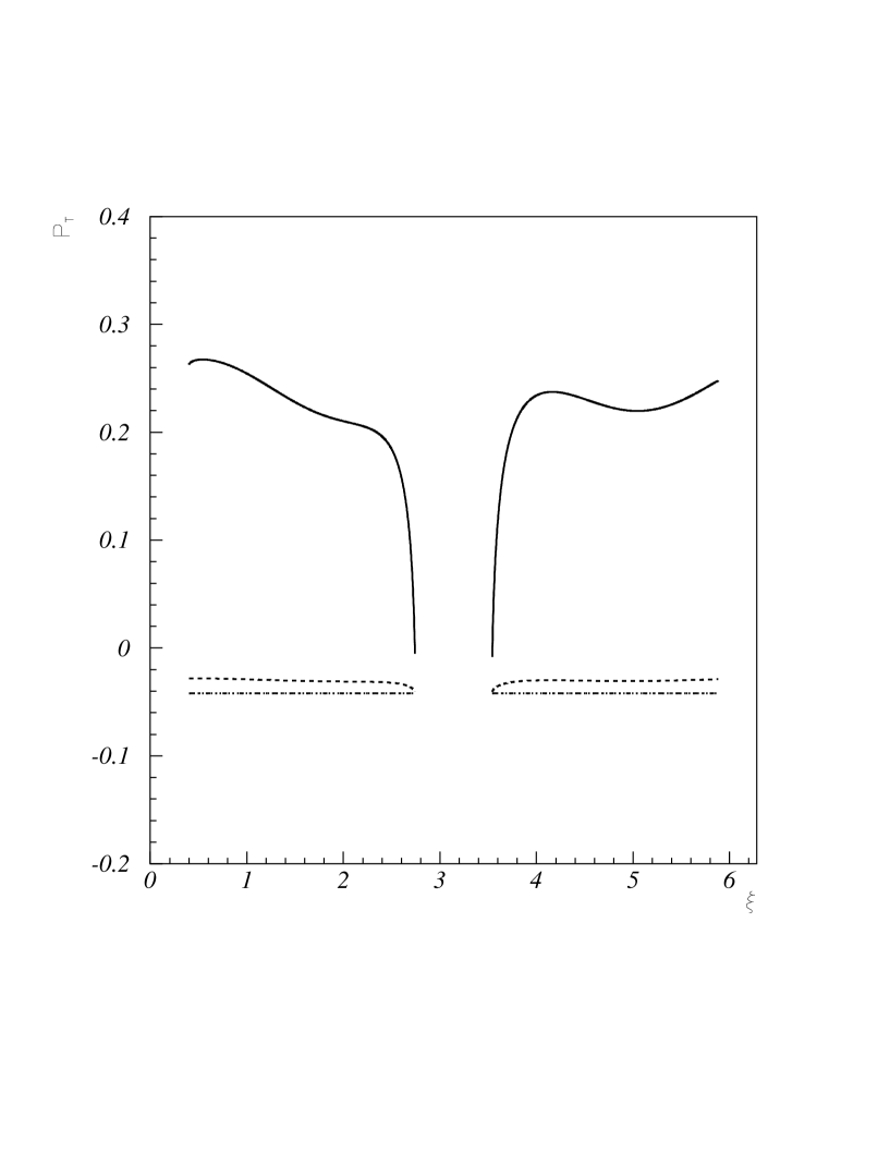
FIG. 10.: $P_{T}$ as function of $\xi$, other captions are same as Fig. 8 (a).

REFERENCES

• [1] D. Hitlin (BaBar Collaboration) and H. Aihara (Belle Collaboration), in the Proceedings (ICHEP2000) edited by C.S. Lim, T. Yamanaka, Singapore, World Scientific, 2001.
• [2] A. Alavi-Harati et al., Phys. Rev. Lett. 83 (1999) 22; G.D. Barr et al., NA31 collaboration, Phys. Lett. B317 (1993) 233; V. Fanti et al. [NA48 Collaboration], Phys. Lett. B 465, 335 (1999) [arXiv:hep-ex/9909022].
• [3] T. D. Lee, Phys. Rev. D8 (1973) 1226; Phys. Rep. 9c (1974) 143; P. Sikivie, Phys. Lett. B65 (1976) 141.
• [4] S. Weinberg, Phys. Rev. Lett. 37 (1976) 657; G. C. Branco, Phys. Rev. D22 (1980) 2901; K. Shizuya and S.-H. H. Tye, Phys. Rev. D23 (1981) 1613.
• [5] Chao-Shang Huang and Shou Hua Zhu, Phys. Rev. D61 (2000) 015011, E: D61 (2000) 119903.
• [6] I. Vendramin, hep-ph/9909291.
• [7] H. Georgi, Hadronic Jour. 1 (1978) 155.
• [8] B.Grinstein, M.J.Savage and M.B.Wise, Nucl.Phys.B319 (1989)271.
• [9] C.S. Huang, W. Liao and Q.S. Yan, Phys. Rev. D59 (1999) 011701; T. Goto, Y. Y. Keum, T. Nihei, Y. Okada and Y. Shimizu, Phys. Lett. B 460, 333 (1999) [arXiv:hep-ph/9812369]; S. Baek and P. Ko, Phys. Lett. B 462, 95 (1999) [arXiv:hep-ph/9904283]; Y.G. Kim, P. Ko and J.S. Lee, Nucl. Phys. B544 (1999) 64; C.W. Bauer, C.N. Burrell, Phys. Rev. D62 (2000) 114028; E. Gabriclli and S. Khalil, hep-ph/0201049. For the earlier references, see, for example, the references in ref. [12] and [17].
• [10] J. L. Hewett, Phys. Rev. D53 (1996) 4964.
• [11] Y. Grossman, Z. Ligeti and E. Nardi, Phys. Rev. D55 (1997) 2768.
• [12] Y.B. Dai, C.S. Huang and H.W. Huang, Phys. Lett. B390 (1997) 257, E: B513 (2001) ; C.S. Huang and Q.S. Yan, Phys. Lett. B442 (1998) 209.
• [13] S. Fukae, C. S. Kim and T. Yoshikawa, Phys. Rev. D 61, 074015 (2000) [arXiv:hep-ph/9908229].
• [14] F. Krüger and L.M. Sehgal, Phys. Lett. B380 (1996) 199.
• [15] S. Rai Choudhury, A. Gupta and N. Gaur, Phys. Rev. D 60, 115004 (1999) [arXiv:hep-ph/9902355].
• [16] E. Lunghi and I. Scimemi, Nucl. Phys. B 574, 43 (2000) [arXiv:hep-ph/9912430].
• [17] C.-S. Huang, Nucl. Phys. B (Proc. Suppl.) 93 (2001) 73 and references therein.
• [18] C. Bobeth, T. Ewerth, F. Kruger and J. Urban, Phys. Rev. D 64, 074014 (2001) [arXiv:hep-ph/0104284].
• [19] Z. h. Xiong and J. M. Yang, arXiv:hep-ph/0105260; E.O.Iltan and G.Turan, Phys. Rev. D63 (2001) 115007.
• [20] Z. h. Xiong and J. M. Yang, Nucl. Phys. B 602, 289 (2001) [arXiv:hep-ph/0012217].
• [21] A. Ali and G. Hiller, Eur.Phys.J. C8(1999) 619-629; F. Kruger and L.M. Sehgal, Phys.Rev.D55(1997) 2799.
• [22] J.F.Gunion,H.E.Haber,G.Kane and S.Dawson, The Higgs hunter’s guide (Addison-Wesley, MA, 1990).
• [23] see, for example, Y.L. Wu and L. Woffenstein, Phys. Rev. Lett. 73, 1762 (1994); D. Bowser-Chao, K. Cheung and W. Y. Keung, Phys. Rev. D 59, 115006 (1999) [arXiv:hep-ph/9811235], and references therein.
• [24] N. G. Deshpande and E. Ma, Phys. Rev. D16 (1977) 1583; A. A. Anselm et al., Phys. Lett. B152 (1985) 116; T. P. Cheng and L. F. Li, Phys. Lett. B234 (1990) 165; S. Weinberg, Phys. Rev. Lett. 63 (1989) 2333; X. -G. He and B. H. J. McKellar, Phys. Rev. D42 (1990) 3221; Erratum-ibid D50 (1994) 4719.
• [25] For a comprehensive review, see: M.Neubert, Phys.Rep. 245 (1994) 396.
• [26] I.I.Bigi, M.Shifman, N.G.Vraltsev and A.I.Vainshtein, Phys. Rev.Lett. 71 (1993) 496; B.Blok, L.Kozrakh, M.Shifman and A.I.Vainshtein, Phys.Rev. D49(1994)3356; A.V.Manohar and M.B.Wise, Phys.Rev. D49(1994)1310; S.Balk, T.G.Körner, D.Pirjol and K.Schilcher, Z. Phys. C64(1994)37; A.F.Falk, Z.Ligeti, M.Neubert and Y.Nir, Phys.Lett. B326(1994) 145.
• [27] H. E. Logan and U. Nierste, Nucl. Phys. B 586, 39 (2000) [arXiv:hep-ph/0004139].
• [28] C.-S. Huang, W. Liao and Q.-S. Yan, S.-H. Zhu, Phys. Rev. D63 (2001) 114021, E: D64 (2001) 059902.
• [29] N. G. Deshpande, J. Trampetic and K. Ponose, Phys. Lett. B214 (1988) 467, Phys. Rev. D39 (1989) 1461; C.S.Lim, T.Morozumi and A.I.Sanda, Phys.Lett.B218 (1989)343; A. Ali, T. Mannel and T. Morozumi, Phys. Lett. B273 (1991) 505; P. J. O’Donnell and H. K. Tung, Phys. Rev. D43 (1991) R2067; G. Buchalla, A. Buras, M. Lautenbacher, Rev. Mod. Phys. 68, (1996) 1125; C. S. Kim, T. Morozumi and A. I. Sanda, Phys. Rev. D56 (1997) 7240.
• [30] N. G. Deshpande and J. Trampetic, Phys. Rev. D60 (1988) 2583; A. J. Buras and M. M$\ddot{u}$nz, Phys. Rev. D52 (1995) 186; A. Ali, G. F. Giudice, and T. Mannel, Z. Phys. C67 (1995) 417.
• [31] Particle Data Group, C. Caso et. al., Eur. Phys. J. C3 (1998)1.
• [32] M. Misiak, Nucl. Phys. B393 (1993) 23; E: B439 (1995) 461; A.J. Buras and M. Münz, Phys. Rev. D52 (1995). Recently, the NNLO corrections in SM have been given: C. Bobeth, M. Misiak and J. Urban, Nucl. Phys. B574 (2000) 291; H.H. Asatryan, H.M. Asatrian, C. Greub and M. walker, hep-ph/0109140.
• [33] C.S.Huang, Commun. Theor. Phys. 2(1983)1265.
• [34] R. Garisto, Phys. Rev. D51 (1995) 1107.
• [35] R. Garisto and G. Kane, Phys. Rev. D44 (1991) 2038.
• [36] ALEPH Collaboration (D. Buskulic et al.), Phys. Lett. B343 (1995)444; J.Kalinowski, Phys.Lett. B245 (1990) 201; A.K.Grant, Phys.Rev. D51 (1995) 207.
• [37] M. Ciuchini, G. Degrassi, P. Gambino and G. F. Giudice, Nucl. Phys. B 527, 21 (1998) [arXiv:hep-ph/9710335]; F. M. Borzumati and C. Greub, Phys. Rev. D 58, 074004 (1998) [arXiv:hep-ph/9802391].
• [38] C. Huang, T. Li, W. Liao, Q. Yan and S. H. Zhu, Eur. Phys. J. C 18, 393 (2000) [hep-ph/9810412].
• [39] S. Bertolini et al., Phys. Rev. Lett. 59 (1987) 180; N. Deshpande et al., ibid., 59 (1987) 183; B. Grinstein et al. Phys. Lett. B202 (1988) 138; R. Grigjanis et al., ibid, 224 (1989) 209; G. Cell et al., ibid, 248 (1990) 181; B. Grinstein et al., Nucl. Phys., B339 (1990) 269;
• [40] A.J. Buras, hep-ph/9806471, and the references therein.
• [41] CLEO Collaboration, hep-ex/9908022; ALEPH Collabration, Phys. Lett. B429, 169 (1998).
• [42] Belle Progress Report, Belle Collaboration, KEK- PROGRESS-REPORT-97-1 (1997); Status of the BaBar Detector, BaBar Collaboration, SLAC-PUB-7951, presented at 29th International Conference on High Energy Physics, Vancouver, Canada, 1998.
Refer to caption