Soliton Models for the Nucleon and Predictions for the Nucleon Spin Structure

Abstract

In these lectures the three flavor soliton approach for baryons is reviewed. Effects of flavor symmetry breaking in the baryon wave–functions on axial current matrix elements are discussed. A bosonized chiral quark model is considered to outline the computation of spin dependent nucleon structure functions in the soliton picture.

1 Introduction

Many nucleon properties cannot be computed from first principles even though the fundamental theory that describes the strong interaction processes of hadrons, Quantum Chromodynamics (QCD), is well established. In QCD hadrons are composites of quarks and gluons whose interactions are described within the non–abelian gauge theory of color $SU(3)$. However, perturbative techniques are not applicable in the low–energy region. It is therefore mandatory to consider models which can be deduced or at least motivated from QCD. In this context it has been fruitful to observe that QCD contains a hidden expansion parameter, $N_{C}$, the number of colors. Generalizing from $SU(3)$ to $SU(N_{C})$ and assuming the confinement phenomena, QCD becomes equivalent to a theory of weakly interacting mesons in the limit of large $N_{C}$ [1]. That is, the coupling constants of the meson interactions scale like $1/N_{C}$ while baryon masses and radii scale like $N_{C}$ and $N_{C}^{0}$, respectively [2]. Meson Lagrangians may possess localized solutions to the field equations with finite field energy, the so–called solitons. Soliton energies scale inversely with the meson coupling and their extensions approach constants as the coupling increases. It was thus conjectured that baryons emerge as solitons in the effective meson theory that is equivalent to QCD [2]. Although this meson theory cannot be derived from QCD, low–energy meson phenomenology provides sufficient constraints to model this theory. Especially chiral symmetry and its breaking in the vacuum are essential. This introduces non–linear interactions for the pions, the (would–be) Goldstone bosons of chiral symmetry, via the chiral field

$$U={\rm exp}\left(i\vec{\tau}\cdot\vec{\pi}/f\right)\,.$$ (1)

Effective Lagrangians are constructed from $U$ that are invariant under global chiral transformations $U\to LUR^{\dagger}$. As $U^{\dagger}U=1$ at least two derivatives are required

$${\cal L}_{0}=\frac{f^{2}}{4}{\rm tr}\left(\partial_{\mu}U\partial^{\mu}U^{\dagger}\right)\,.$$ (2)

Extracting the axial current $A_{\mu}^{a}=f\pi^{a}+{\cal O}(\vec{\pi}\hskip 0.56905pt^{3})$ from ${\cal L}_{0}$ provides the electroweak coupling and determines the pion decay constant $f=f_{\pi}=93{\rm MeV}$ from $\pi\to\mu\nu$. Having established such a chiral model, a finite energy soliton solution must be obtained and quantized to describe baryon states. I will outline this approach in section 2. In section 3 I will consider three flavor extensions thereof with special emphasis on the role of flavor symmetry breaking [3]. I will employ these methods to compute axial current matrix elements of baryons in section 4. These matrix elements are essential ingredients for the description of the nucleon spin structure [4] as they reflect its various quark flavor contributions [5] and they parameterize hyperon beta–decay. The effects of flavor symmetry breaking will be essential to discuss the strange quark contribution. In section 5 I will discuss a different approach by starting from a simple model for the quark flavor dynamics. Using standard bosonization techniques [6] this model is rewritten as a (non–local) meson field theory which can be shown to support chiral solitons [7]. As I will describe in sections 6 and 7, the quark degrees of freedom can be traced through the bosonization procedure for the amplitude of virtual Compton scattering. This paves the way to compute nucleon structure functions from the chiral quark soliton. Finally section 8 contains some concluding remarks.

2 Baryons as Chiral Solitons

Scaling considerations show that the model (2) does not contain stable soliton solutions. Therefore Skyrme added a stabilizing term [8]

$${\cal L}=\frac{f_{\pi}^{2}}{4}{\rm tr}\left[\partial_{\mu}U\partial^{\mu}U^{\dagger}\right]+\frac{1}{32e^{2}}{\rm tr}\left(\left[U^{\dagger}\partial_{\mu}U,U^{\dagger}\partial_{\nu}U\right]\left[U^{\dagger}\partial^{\mu}U,U^{\dagger}\partial^{\nu}U\right]\right)\,,$$ (3)

that is of fourth order in the derivatives but only quadratic in the time derivatives. There are other approaches to extend ${\cal L}_{0}$ such that stable soliton solutions exist, as e.g. including vector mesons [9, 10]. Although such extensions appear physically more motivated, I will stick to the Skyrme model for pedagogical reasons when explaining the soliton picture for baryons.

The soliton solution to (3) assumes the famous hedgehog shape

$$U_{\rm H}\left(\vec{r}\,\right)={\rm exp}\left(i\vec{\tau}\cdot\hat{r}F(r)\right)\,.$$ (4)

The equations of motion become an ordinary second order differential equation for the chiral angle $F(r)$ that are obtained by extremizing the classical energy

$$E_{\rm cl}=E_{\rm cl}[F]=\int d^{3}r\left\{\frac{f_{\pi}^{2}}{2}\left(r^{2}F^{\prime 2}+2{{\rm sin}^{2}}F\right)+\frac{{{\rm sin}^{2}}F}{2e^{2}}\left(2F^{\prime 2}+\frac{{{\rm sin}^{2}}F}{r^{2}}\right)\right\}\,.$$ (5)

It can be argued [11] that the baryon number equals the winding number associated with the mapping (4), i.e. $B=[F(\infty)-F(0)]/\pi$. Hence the boundary conditions $F(0)=-\pi$ and $F(\infty)=0$ corresponding to unit baryon number determine the chiral angle uniquely. This soliton does not yet describe states of good spin and/or flavor as the ansatz (4) does not possess the corresponding symmetries. Such states are generated by restoring these symmetries through collective coordinates $A(t)$

$$U(\vec{r},t)\,=\,A(t)\,U_{\rm H}(\vec{r})\,A^{\dagger}(t)\,.$$ (6)

and subsequent canonical quantization thereof [12]. This introduces right $[A,R_{i}]=A\tau_{i}/2$ and left generators $[A,L_{i}]=\tau_{i}A/2$. While the isospin interpretation $I_{i}=L_{i}$ is general, the identity $J_{i}=-R_{i}$ for the spin is due to the hedgehog structure (4) as is the relation $|\vec{I}|=|\vec{J}|$. By quantizing the collective coordinates one obtains a Hamiltonian in terms of physical observables

$$H_{\rm coll}\,=\,E_{\rm cl}+\frac{\vec{J}\,^{2}}{2\alpha^{2}}\,=\,E_{\rm cl}+\frac{\vec{I}\,^{2}}{2\alpha^{2}}\,.$$ (7)

The moment of inertia is also a functional of the above determined chiral angle

$$\alpha^{2}[F]=\frac{2}{3}\int d^{3}r\,{\rm sin}^{2}F\left[f_{\pi}^{2}+\frac{1}{e^{2}}\left(F^{\prime 2}+\frac{{\rm sin}^{2}F}{r^{2}}\right)\right]\,.$$ (8)

Matching the empirical mass difference $M_{\Delta}-M_{\rm N}=\frac{3}{2\alpha^{2}}\sim 300{\rm MeV}$ fixes the so–far undetermined parameter to be $e\approx 4.0$.

3 Extension to Three Flavors

The generalization to three flavors is carried out straightforwardly by taking $A(t)\in SU(3)$ with the hedgehog (4) embedded in the isospin subgroup. However, the Lagrangian becomes more complicated as there are two essential extensions. The first one is the Wess–Zumino–Witten term [11]. Gauging it for local $U_{V}(1)$ shows that indeed the winding number current equals the baryonic current. Furthermore, as it is linear in the time derivative it constrains $A$ to be quantized as a fermion (for $N_{C}$ odd). The second extension originates from flavor symmetry breaking that is reflected by different masses and decay constants of the pseudoscalar mesons

$${\cal L}_{\rm SB}=\frac{f_{\pi}^{2}m_{\pi}^{2}-f_{K}^{2}M_{K}^{2}}{2\sqrt{3}}{\rm tr}\left\{\lambda_{8}\left(U+U^{\dagger}\right)\right\}+\frac{f_{K}^{2}-f_{\pi}^{2}}{4\sqrt{3}}{\rm tr}\left\{\lambda_{8}\left(\partial_{\mu}U\partial^{\mu}U^{\dagger}U+{\rm h.c.}\right)\right\}\,.$$ (9)

The explicit form of ${\cal L}_{\rm SB}$ is model dependent, however, the techniques to study its effects on baryon properties are general.

In $SU(3)$ the collective coordinates are parameterized by eight “Euler–angles”

$$A=D_{2}(\hat{I})\,{\rm e}^{-i\nu\lambda_{4}}D_{2}(\hat{R})\,{\rm e}^{-i(\rho/\sqrt{3})\lambda_{8}}\ ,$$ (10)

where $D_{2}$ denote rotation matrices of three Euler–angles for each, rotations in isospace ($\hat{I}$) and coordinate–space ($\hat{R}$). Substituting the ansatz (6) into ${\cal L}+{\cal L}_{\rm SB}$ yields upon canonical quantization the Hamiltonian for the collective coordinates $A$:

$$H=H_{\rm s}+{\textstyle\frac{3}{4}}\,\gamma\,{\rm sin}^{2}\nu\,.$$ (11)

The symmetric piece of this collective Hamiltonian only contains Casimir operators and may be expressed in terms of the $SU(3)$–right generators $R_{a}\,(a=1,\ldots,8)$:

$$H_{\rm s}=E_{\rm cl}+\frac{1}{2\alpha^{2}}\sum_{i=1}^{3}R_{i}^{2}+\frac{1}{2\beta^{2}}\sum_{\alpha=4}^{7}R_{\alpha}^{2}\,.$$ (12)

While $\beta^{2}$ is a moment of inertia similar to $\alpha^{2}$ in eq (8), $\gamma=\gamma[F]$ completely originates from symmetry breaking

$$\gamma=\frac{2\pi}{3}\int d^{3}r\left[\left(f_{K}^{2}m_{K}^{2}-f_{\pi}^{2}m_{\pi}^{2}\right)\left(1-{\rm cos}F\right)+\frac{f_{K}^{2}-f_{\pi}^{2}}{2}{\rm cos}F\left(F^{\prime 2}r^{2}+2{\rm sin}^{2}F\right)\right].$$

The generators $R_{a}$ can be expressed in terms of derivatives with respect to the ‘Euler–angles’. The eigenvalue problem $H\Psi=\epsilon\Psi$ reduces to sets of ordinary second order differential equations for isoscalar functions which only depend on the strangeness changing angle $\nu$ [13] that can be integrated numerically. Only the product $\omega^{2}=\frac{3}{2}\gamma\beta^{2}$ appears in these differential equations which is thus interpreted as the effective strength of the flavor symmetry breaking. A value in the range $5{{\stackrel{{\scriptstyle\scriptscriptstyle\raisebox{-7.11317pt}{$<$}}}{{\scriptscriptstyle\raisebox{-2.27621pt}{$\sim$}}}}}\omega^{2}{{\stackrel{{\scriptstyle\scriptscriptstyle\raisebox{-7.11317pt}{$<$}}}{{\scriptscriptstyle\raisebox{-2.27621pt}{$\sim$}}}}}8$ is required to obtain reasonable agreement with the empirical mass differences for the $\frac{1}{2}^{+}$ and $\frac{3}{2}^{+}$ baryons [3]. The eigenstates of the symmetric piece (12) are members of definite $SU(3)$ representations, e.g. the octet (8) for the low–lying $\frac{1}{2}^{+}$ baryons. Upon flavor symmetry breaking, states of different representations are mixed. At $\omega^{2}=6$ the nucleon amplitude contains a 23% contamination of the state with nucleon quantum numbers in the ${\bf\bar{10}}$ representation. That is, the baryon wave–functions exhibit strong distortion from flavor covariance. It is interesting to see what influence this has for baryon properties, in particular the hyperon beta–decay for which flavor covariance is known to work very well [14].

4 Axial Current Matrix Elements

Table 1. : The empirical values for the $g_{A}/g_{V}$ ratios of hyperon beta–decays [15]. For the process $\Sigma\to\Lambda$ only $g_{A}$ is given. Also the flavor symmetric predictions are presented using the values for $F$&$D$ of Ref. [14].

	$\Lambda\to p$	$\Sigma\to n$	$\Xi\to\Lambda$	$\Xi\to\Sigma$	$\Sigma\to\Lambda$
emp.	$0.718\pm 0.015$	$0.340\pm 0.017$	$0.25\pm 0.05$	$1.287\pm 0.158$	$0.61\pm 0.02$
$F$&$D$	$0.725\pm 0.009$	$0.339\pm 0.026$	$0.19\pm 0.02$	$1.258=g_{A}$	$0.65\pm 0.01$

The effect of the derivative type symmetry breaking terms is mainly indirect. They provide the splitting between the various decay constants and thus increase $\gamma$ because of $f_{K}^{2}m_{K}^{2}-f_{\pi}^{2}m_{\pi}^{2}\approx 1.5f_{\pi}^{2}(m_{K}^{2}-m_{\pi}^{2})$. Otherwise the terms proprotional to $f_{K}^{2}-f_{\pi}^{2}$ may be omitted. Whence there are no symmetry breaking terms in current operators and the non–singlet axial charge operator is parameterized as

$$\int d^{3}rA_{i}^{(a)}=c_{1}D_{ai}-c_{2}D_{a8}R_{i}+c_{3}\sum_{\alpha,\beta=4}^{7}d_{i\alpha\beta}D_{a\alpha}R_{\beta}\,,$$ (13)

where $D_{ab}=\frac{1}{2}{\rm tr}\left(\lambda_{a}A\lambda_{b}A^{\dagger}\right)$, $a=1,\ldots,8$ and $i=1,2,3$. In the limit $\omega^{2}\to\infty\,$ (integrating out strange degrees of freedom) the strangeness contribution to the axial charge of the nucleon should vanish. As the baryon wave–functions parameterically depend on $\omega^{2}$ one finds $\langle N|D_{83}|N\rangle\to 0$ and $\langle N|\sum_{\alpha,\beta=4}^{7}d_{3\alpha\beta}D_{8\alpha}R_{\beta}|N\rangle\to 0$ while $\langle N|D_{88}|N\rangle\to 1$ for $\omega^{2}\to\infty$. Thus the above consistency condition requires

$$\int d^{3}rA_{i}^{(0)}=-2\sqrt{3}c_{2}R_{i}\quad i=1,2,3\,.$$ (14)

for the singlet axial current because it yields a vanishing strangeness projection, $A_{i}^{(s)}=(A_{i}^{(0)}-2\sqrt{3}A_{i}^{(8)})/3$ for $\omega^{2}\to\infty$. Note that the appearance of $c_{2}$ in eq (14) goes beyond group theoretical arguments. Actually all model calculations in the literature [16, 17] are consistent with (14). In order to completely describe the hyperon beta–decays we also demand matrix elements of the vector charges. These are obtained from the operator

$$\int d^{3}rV_{0}^{(a)}=\sum_{b=1}^{8}D_{ab}R_{b}=L_{a},$$ (15)

which introduces the $SU(3)$–left generators $L_{a}$.

The values for $g_{A}$ and $g_{V}$ (only $g_{A}$ for $\Sigma^{+}\to\Lambda e^{+}\nu_{e}$) are obtained from the matrix elements of respectively the operators in eqs (13) and (15), sandwiched between the eigenstates of the full Hamiltonian (11). I choose $c_{2}$ according to $\langle N|\int d^{3}rA_{3}^{(0)}|N\rangle=-\sqrt{3}c_{2}=\Delta\Sigma=0.2\pm 0.1$ [5] and subsequently determine $c_{1}$ and $c_{3}$ at $\omega^{2}_{\rm fix}=6.0$ such that the emprical values for the nucleon axial charge, $g_{A}$ and the $g_{A}/g_{V}$ ratio for $\Lambda\to pe^{-}\bar{\nu}_{e}$ are reproduced. This not only predicts the other decay parameters but also describes the variation with symmetry breaking as shown in figure 1.

         

         

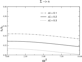
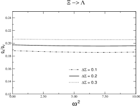
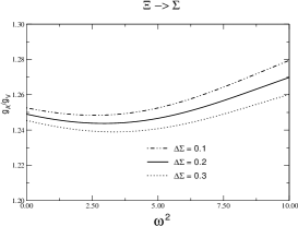
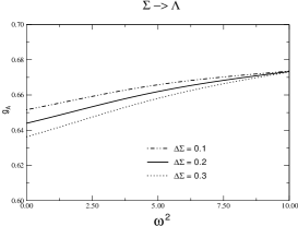
Fig. 1. : The predicted decay parameters for the hyperon beta–decays using $\omega^{2}_{\rm fix}=6.0$. The errors originating from those in $\Delta\Sigma_{N}$ are indicated.

The dependence on flavor symmetry breaking is very moderate and the results can be viewed as reasonably agreeing with the empirical data, cf. table 1. The two transitions, $n\to p$ and $\Lambda\to p$, which are not shown in figure 1, exhibit a similar neglegible dependence on $\omega^{2}$. The observed independence of $\omega^{2}$ shows that these predictions are not sensitive to the choice of $\omega^{2}_{\rm fix}$. Comparing the results in figure 1 with the data in table 1 shows that the calculation using the strongly distorted wave–functions agrees equally well with the empirical data as the flavor symmetric $F$&$D$ fit.

         

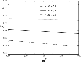
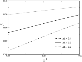
Fig. 2. : The contributions of the non–strange (left panel) and strange (right panel) degrees of freedom to the axial charge of the $\Lambda$. Again $\omega^{2}_{\rm fix}=6.0$ was assumed.

Figure 2 shows the flavor components of the axial charge of the $\Lambda$ hyperon. Again, the various contributions to the axial charge of the $\Lambda$ exhibit only a moderate dependence on $\omega^{2}$. The non–strange component, $\Delta U_{\Lambda}=\Delta D_{\Lambda}$ slightly increases in magnitude. The strange quark piece, $\Delta S_{\Lambda}$ grows with symmetry breaking since $\Delta\Sigma_{\Lambda}$ is kept fixed. These results agree nicely with an $SU(3)$ analysis applied to the data [19]. The observed independence on $\omega^{2}$ does not occur for all matrix elements of the axial current. A prominent exemption is the strange quark component in the nucleon, $\Delta S_{N}$. For $\Delta\Sigma=0.2$, say, it is significant at zero symmetry breaking, $\Delta S_{N}=-0.131$ while it decreases (in magnitude) to $\Delta S_{N}=-0.085$ at $\omega^{2}=6.0$.

This far I have only considered the general sturcture of the current operators in soliton models without actually computing the constants $c_{i}$ from a model soliton, although I had the Skyrme model in mind. However, this model is too simple to be realistic. For example, it improperly predicts $\Delta\Sigma=0$ [3] and more complicted models must be utilized, as e.g. the vector meson model that has been established for two flavors in ref [9]. Later it has been generalized to three flavors and been shown to fairly describe hyperon beta–decay [16]. A minimal set of symmetry breaking terms is included [20] to account for different masses and decay constants. These terms add symmetry breaking pieces to the axial charge operator,

$$\delta A_{i}^{(a)}=c_{4}D_{a8}D_{8i}+c_{5}\sum_{\alpha,\beta=4}^{7}d_{i\alpha\beta}D_{a\alpha}D_{8\beta}+c_{6}D_{ai}(D_{88}-1)\,\,,\,\delta A_{i}^{(0)}=2\sqrt{3}\,c_{4}D_{8i}\,.$$

The coefficients $c_{1},\ldots,c_{6}$ are functionals of the soliton and can be computed once the soliton is constructed [18]. As the model parameters cannot be completely determined in the meson sector [9] I use the small remaining freedom to accommodate baryon properties in three different ways, see table 2. The set denoted by ‘masses’ refers to a best fit to the baryon mass differences. It predicts the axial charge somewhat on the low side, $g_{A}=0.88$. The set named ‘mag.mom.’ refers to parameters that yield magnetic moments of the $\frac{1}{2}^{+}$ baryons close to the respective empirical data (with $g_{A}=0.98$) and finally the set labeled ‘$g_{A}$’ reproduces the axial charge of the nucleon and also reasonably accounts for hyperon beta–decay [16].

Table 2. : Spin content of the $\Lambda$ in the realistic vector meson model. For comparison the nucleon results are also given. Three sets of model parameters are considered, see text.

	$\Lambda$			$N$
	$\Delta U=\Delta D$	$\Delta S$	$\Delta\Sigma$	$\Delta U$	$\Delta D$	$\Delta S$	$\Delta\Sigma$
masses	$-0.155$	$0.567$	$0.256$	$0.603$	$-0.279$	$-0.034$	$0.291$
mag. mom.	$-0.166$	$0.570$	$0.238$	$0.636$	$-0.341$	$-0.030$	$0.265$
$g_{A}$	$-0.164$	$0.562$	$0.233$	$0.748$	$-0.476$	$-0.016$	$0.256$

As presented in table 2, the predictions for the axial properties of the $\Lambda$ are insensitive to the model parameters. The singlet matrix element of the $\Lambda$ hyperon is smaller than that of the nucleon. Sizable polarizations of the up and down quarks in the $\Lambda$ are predicted. They are slightly smaller in magnitude but nevertheless comparable to those obtained from the $SU(3)$ symmetric analyses [19].

5 Solitons in a Chiral Quark Model

In the preceding discussions I have illuminated the success of the soliton picture using hyperon–beta decay and axial current matrix elements as examples. To study those processes it was sufficient to consider static baryon properties as computed from a purely meson model Lagrangian. In order to advance and compute structure functions as they are measured in deep inelastic scattering (DIS) in the soliton picture it will be necessary to trace the quark degrees of freedom as the meson model is constructed. As already mentioned, this cannot be accomplished in QCD and therefore I will utilize a simpler model of the quark flavor dynamics. Integrating out the quark degrees gives a bosonized action that can be cast in the form

$${\cal A}[S,P]=-iN_{C}{\rm Tr}_{\textstyle\Lambda}{\rm log}\,\left[i\partial\hskip-5.0pt/-\left(S+i\gamma_{5}P\right)\right]-\frac{1}{4G}\int d^{4}x\,{\rm tr}\,{\cal V}(S,P)\,.$$ (16)

Here ${\cal V}$ is a local potential respectively for scalar and pseudoscalar fields $S$ and $P$ which are matrices in flavor space. For example, in the Nambu–Jona–Lasinio (NJL) model [21] one has ${\cal V}=S^{2}+P^{2}+2{\hat{m}}_{0}S$ with $\hat{m}_{0}$ being the current quark mass matrix. The functional trace (${\rm Tr}$) refects integrating out the quarks and induces a non–local interaction for $S$ and $P$. A major concern in regularizing the functional (16), as indicated by the cut–off $\Lambda$, is to maintain the chiral anomaly. This is achieved by splitting this functional into $\gamma_{5}$–even and odd pieces via

$${\rm Tr}_{\Lambda}{\rm log}\,\left[i\partial\hskip-5.0pt/-\left(S+i\gamma_{5}P\right)\right]=-i\frac{N_{C}}{2}\sum_{i=0}^{2}c_{i}{\rm Tr}\,{\rm log}\left[-{\bf D}{\bf D}_{5}+\Lambda_{i}^{2}-i\epsilon\right]\hskip 36.13512pt$$ (17)

$$\hskip 142.26378pt-i\frac{N_{C}}{2}{\rm Tr}\,{\rm log}\left[-{\bf D}\left({\bf D}_{5}\right)^{-1}-i\epsilon\right]\,,\hskip 28.45274pt$$

$${\rm with} \qquad i{\bf D}=i\partial\hskip-5.0pt/-\left(S+i\gamma_{5}P\right)\quad{\rm and}\quad i{\bf D}_{5}=-i\partial\hskip-5.0pt/-\left(S-i\gamma_{5}P\right)\,.$$ (18)

With the conditions $c_{0}=1\,,\,\,\Lambda_{0}=0,\,\sum_{i=0}^{2}c_{i}=0\,{\rm and}\,\sum_{i=0}^{2}c_{i}\Lambda_{i}^{2}=0$ the double Pauli–Villars regularization renders the functional (16) finite. The $\gamma_{5}$–odd piece is conditionally finite and not regularizing it properly reproduces the chiral anomaly. For sufficiently large $G$ one obtains the VEV, $\langle S\rangle\equiv m\neq 0$ that parameterizes the dynamical chiral symmetry breaking from the gap–equation.

Before discussing nucleons as solitons of the bosonized action (16) and the respective structure functions it will be illuminating to first consider DIS off pions. Details of these studies are published in [22]. For related work see refs [23, 24, 25].

6 The Compton Tensor and Pion Structure Function

DIS off hadrons is parameterized by the hadronic tensor $W^{\mu\nu}(q)$ with $q$ being the momentum transmitted to the hadron by the photon. $W^{\mu\nu}(q)$ is obtained from the hadron matrix element of the commutator $[J^{\mu}(\xi),J^{\nu}(0)]$. An essential feature of bosonized quark models is that the derivative term in (16) is formally identical to that of a non–interacting quark model. Hence the current operator is given as $J^{\mu}={\bar{q}}{\cal Q}\gamma^{\mu}q$, with ${\cal Q}$ being a flavor matrix. Expectation values of currents are computed by introducing pertinent sources $v_{\mu}$ in eq (17)

$$i{\bf D}\,\longrightarrow\,i{\bf D}+{\cal Q}v\hskip-5.0pt/\qquad{\rm and}\qquad i{\bf D}_{5}\,\longrightarrow\,i{\bf D}_{5}-{\cal Q}v\hskip-5.0pt/$$ (19)

and taking appropriate derivatives. In bosonized quark models it is convenient to start from the absorptive part of the forward virtual Compton amplitude

$$T^{\mu\nu}(q)=\int d^{4}\xi\,{\rm e}^{iq\cdot\xi}\,\langle p,s|T\left(J^{\mu}(\xi)J^{\nu}(0)\right)|p,s\rangle\quad{\rm and}\quad W^{\mu\nu}(q)=\frac{1}{2\pi}\Im\,(T^{\mu\nu}(q)\,.$$ (20)

because the time–ordered product is unambiguously obtained from

$$T\left(J^{\mu}(\xi)J^{\nu}(0)\right)=\frac{\delta^{2}}{\delta v_{\mu}(\xi)\,\delta v_{\nu}(0)}\,{\rm Tr}_{\Lambda}{\rm log}\,\left[i\partial\hskip-5.0pt/-\left(S+i\gamma_{5}P\right)+{\cal Q}\,v\hskip-5.0pt/\right]\Big{|}_{v_{\mu}=0}\,\,,$$ (21)

as defined from eqs (17) with the substitution (19). In order to extract the leading twist pieces of the structure functions, $W^{\mu\nu}(q)$ is studied in the Bjorken limit: $q^{2}\to-\infty$ with $x=-q^{2}/p\cdot q$ fixed.

DIS off pions is characterized by a single structure function, $F(x)$. For its computation the pion matrix element in the Compton amplitude (20) must be specified. Whence I introduce the pion field ${\vec{\pi}}$ via

$$S+iP\gamma_{5}=m\,\left(U\right)^{\gamma_{5}}=m\,{\rm exp}\left(i\frac{g}{m}\gamma_{5}\,{\vec{\pi}}\cdot{\vec{\tau}}\right)\,.$$ (22)

In a first step pion properties are utilized to fix the model parameters. It is also worthwhile to mention that expanding (17,22) to linear and quadratic order in $\vec{\pi}$ and $v_{\mu}$, respectively yields the proper result for the anomalous decay $\pi^{0}\to\gamma\gamma$. The Compton amplitude for virtual pion–photon scattering is obtained by expanding (17,22) to second order in both, ${\vec{\pi}}$ and $v_{\mu}$. Due to the separation into ${\bf D}$ and ${\bf D}_{5}$ this calculation differs considerably from the evaluation of the ‘handbag’ diagram because isospin violating dimension–five operators emerge. Fortunately all isospin violating pieces cancel yielding

$$F(x)=\frac{5}{9}(4N_{C}g^{2})\frac{d}{dm_{\pi}^{2}}\left\{m_{\pi}^{2}\sum_{i=0}^{2}c_{i}\,\frac{d^{4}k}{(2\pi)^{4}i}\,\left[k^{2}+x(1-x)m_{\pi}^{2}-m^{2}-\Lambda_{i}^{2}+i\epsilon\right]^{-2}\right\}\,.$$

The cancellation of the isospin violating pieces is a feature of the Bjorken limit: insertions of the pion field on the propagator carrying the infinitely large photon momentum can be safely ignored. Furthermore this propagator can be taken to be the one for non–interacting massless fermions. This implies that also the Pauli–Villars cut–offs can be omitted for this propagator leading to the desired scaling behavior of the structure function.

7 Nucleon Structure Functions

Assuming the hedgehog shape (4) for the pion field (22) the profile function $F(r)$ enters the single particle Dirac Hamiltonian

$$h=\vec{\alpha}\cdot\vec{p}+\beta\,m\,\left[{\rm cos}F+i\gamma_{5}\vec{\tau}\cdot\hat{r}\,{\rm sin}F\right]\,.$$ (23)

Denoting its eigenvalues with $\epsilon_{\alpha}$ allows one to construct an energy functional [26]

$$E[F] = \frac{N_{C}}{2}\left(1-{\rm sign}(\epsilon_{\rm val})\right)\epsilon_{\rm val}-\frac{N_{C}}{2}\sum_{i=0}^{2}c_{i}\sum_{\alpha}\left\{\sqrt{\epsilon_{\alpha}^{2}+\Lambda_{i}^{2}}-\sqrt{\epsilon_{\alpha}^{(0)2}+\Lambda_{i}^{2}}\right\}$$ (24)

$$\hskip 56.9055pt+m_{\pi}^{2}f_{\pi}^{2}\int d^{3}r\,(1-{\rm cos}F)\,$$

for a unit baryon number configuration. Here $\epsilon_{\rm val}$ denotes the unique bound state level and $\epsilon_{\alpha}^{(0)}$ are the eigenvalues when the soliton is absent. The soliton profile $F(r)$ is then obtained from extremizing $E$ self–consistently [7]. As described in sections 2 and 3, nucleon states are generated by introducing collective coordinates (6) and subsequent canonical quantization thereof [27].

As argued in the previous section the quark propagator with the infinite photon momentum should be taken to be free and massless. Thus, it is sufficient to differentiate (Here ${\bf D}$ and ${\bf D}_{5}$ are those of eq (18), i.e. with $v_{\mu}=0$.)

$$\frac{N_{C}}{4i}\sum_{i=0}^{2}c_{i}{\rm Tr}\,\left\{\left(-{\bf D}{\bf D}_{5}+\Lambda_{i}^{2}\right)^{-1}\left[{\cal Q}^{2}v\hskip-5.0pt/\left(\partial\hskip-5.0pt/\right)^{-1}v\hskip-5.0pt/{\bf D}_{5}-{\bf D}(v\hskip-5.0pt/\left(\partial\hskip-5.0pt/\right)^{-1}v\hskip-5.0pt/)_{5}{\cal Q}^{2}\right]\right\}$$

$$+\frac{N_{C}}{4i}{\rm Tr}\,\left\{\left(-{\bf D}{\bf D}_{5}\right)^{-1}\left[{\cal Q}^{2}v\hskip-5.0pt/\left(\partial\hskip-5.0pt/\right)^{-1}v\hskip-5.0pt/{\bf D}_{5}+{\bf D}(v\hskip-5.0pt/\left(\partial\hskip-5.0pt/\right)^{-1}v\hskip-5.0pt/)_{5}{\cal Q}^{2}\right]\right\}\,,\,\,$$ (25)

with respect to the photon field $v_{\mu}$. I have introduced the $(\ldots)_{5}$ description

$$\gamma_{\mu}\gamma_{\rho}\gamma_{\nu}=S_{\mu\rho\nu\sigma}\gamma^{\sigma}-i\epsilon_{\mu\rho\nu\sigma}\gamma^{\sigma}\gamma^{5}\quad{\rm and}\quad(\gamma_{\mu}\gamma_{\rho}\gamma_{\nu})_{5}=S_{\mu\rho\nu\sigma}\gamma^{\sigma}+i\epsilon_{\mu\rho\nu\sigma}\gamma^{\sigma}\gamma^{5}$$ (26)

to account for the unconventional appearance of axial sources in ${\bf D}_{5}$ [22]. Substituting (6) into (25) and computing the functional trace, using a basis of quark states obtained from the Dirac Hamiltonian (23), yields analytical results for the structure functions. I refer to [22] for detailed formulae and the explicit verification of sum rules. Here I simply report the important result that the structure function entering the Gottfried sum rule is related to the $\gamma_{5}$–odd piece of the action and hence does not undergo regularization. This is surprising because in the parton model this structure function differs from the one associated with the Adler sum rule only by the sign of the anti–quark distribution. The latter structure function, however, gets regularized, in agreement with the quantization rules for the collective coordinates.

Unfortunately numerical results for the full structure functions in the double Pauli–Villars regularization scheme, i.e. including the properly regularized vacuum piece are not yet available. However, in the Pauli–Villars regularization the axial charges are saturated to 95% or more by their valence quark ($\epsilon_{\rm val}$) contributions once the self–consistent soliton is substituted. This provides sufficient justification to adopt the valence quark contribution to the polarized structure functions as a reliable approximation [23]. Note that the zeroth moment of the leading structure function $g_{1}$ is nothing but the axial current matrix elements discussed in section 4. In figure 3 I compare the model predictions for the linearly independent polarized structure functions to experimental data [30].

Fig. 3. : Model predictions for the polarized proton structure functions $xg_{1}$ (left panel) and $xg_{2}$ (right panel). The curves labeled ‘RF’ denote the results as obtained from the valence quark contribution to (25). These undergo a projection to the infinite momentum frame ‘IMF’ [28] and a leading order ‘LO’ DGLAP evolution [29]. Data are from SLAC–E143 [30].

The evolution of the structure function $g_{2}$ to the momentum scale of the experiments requires the separation into twist–2 and twist–3 components [29]. The model results for the polarized structure functions, which I argued to have reliably approximated, agree reasonably well with the experimental data.

8 Conclusions

In these lectures I have discussed a twofold program to study the nucleon spin structure in chiral soliton models. After having reviewed the arguments from large $N_{C}$ QCD that lead to the picture that baryons emerge as solitons in an effective meson theory I have adopted that picture to compute various baryon matrix elements. Here I focused on the effects of flavor symmetry breaking in the baryon wave–functions and showed that despite of strong deviations from flavor covariant wave–functions the empirical parameters for hyperon beta–decay are reproduced. I also showed that chiral soliton models provide a consistent explanation of the proton spin puzzle, i.e. the smallness of the observed axial singlet current matrix element. On the other hand flavor symmetry breaking in the nucleon wave–function leads to a significant reduction of the polarization of the strange quarks inside the nucleon. In the second part of these lectures I describe how an effective meson theory that contains chiral soliton solutions can be constructed from a simplified model for the quark flavor dynamics. Since the quark degrees of freedom can be traced through this bosonization procedure it is possible to compute nucleon structure functions from this soliton. It turns out that additional correlations are introduced due to the unavoidable regularization which is imposed in a way to respect the chiral anomaly. Hence a consistent extraction of the nucleon structure functions from the Compton amplitude in the Bjorken limit leads to expressions that are quite different from those obtained by an ad hoc regularization of quark distributions in the same model. I also showed that within a reliable approximation the numerical results for the spin dependent structure functions agree reasonably well with the empirical data.

I would like to thank Miroslav Finger for organizing this worthwhile Advanced Study Institute. This work has been supported by the Deutsche Forschungsgemeinschaft under contracts We 1254/3-1 and We 1254/4-2.

References

- [1] G. t‘ Hooft, Nucl. Phys. B72 (1974) 461; B75 (1975) 461.
- [2] E. Witten, Nucl. Phys. B160 (1979) 57.
- [3] H. Weigel, Int. J. Mod. Phys. A11 (1996) 2419, J. Schechter and H. Weigel, arXiv:hep-ph/9907554.
- [4] R. L. Jaffe, arXiv:hep-ph/9602236.
- [5] J. R. Ellis and M. Karliner, arXiv:hep-ph/9601280.
- [6] D. Ebert and H. Reinhardt, Nucl. Phys. B271 (1986) 188.
- [7] R. Alkofer, H. Reinhardt and H. Weigel, Phys. Rept. 265 (1996) 139, C. V. Christov et al., Prog. Part. Nucl. Phys. 37 (1996) 91.
- [8] T. H. R. Skyrme, Proc. Roy. Soc. Lond. A 260 (1961) 127.
- [9] P. Jain et al., Phys. Rev. D37 (1988) 3252; Ulf–G. Meißner, N. Kaiser, H. Weigel, and J. Schechter, Phys. Rev. D39 (1989) 1956.
- [10] Ö. Kaymakcalan, S. Rajeev, and J. Schechter, Phys. Rev. D30 (1984) 594.
- [11] E. Witten, Nucl. Phys. B223 (1983) 422, Nucl. Phys. B223 (1983) 433.
- [12] G. S. Adkins, C. R. Nappi, and E. Witten, Nucl. Phys. B228 (1983) 552.
- [13] H. Yabu and K. Ando, Nucl. Phys. B301 (1988) 601.
- [14] R. Flores–Mendieta, E. Jenkins, and A. V. Manohar, Phys. Rev. D58 (1998) 094028.
- [15] C. Caso et al., (Particle Data Group), Eur. Phys. J. C3 (1998) 1; M. Bourquin et al., Z. Phys. C12 (1982) 307; C21 (1983) 1.
- [16] N. W. Park and H. Weigel, Nucl. Phys. A541 (1992) 453.
- [17] A. Blotz, M. Praszałowicz, and K. Goeke, Phys. Lett. B317 (1993) 195.
- [18] H. Weigel, Nucl. Phys. A690 (2001) 595.
- [19] R. L. Jaffe, Phys. Rev. D54 (1996) 6581
- [20] P. Jain et al., Phys. Rev. D40 (1989) 855.
- [21] Y. Nambu and G. Jona–Lasinio, Phys. Rev. 122 (1961) 345; 124 (1961) 246.
- [22] H. Weigel, E. Ruiz Arriola and L. Gamberg, Nucl. Phys. B560 (1999) 383.
- [23] H. Weigel, L. Gamberg and H. Reinhardt, Mod. Phys. Lett. A11 (1996) 3021; Phys. Lett. B399 (1997) 287; Phys. Rev. D55 (1997) 6910; L. Gamberg, H. Reinhardt and H. Weigel, Phys. Rev. D58 (1998) 054014; O. Schröder, H. Reinhardt and H. Weigel, Phys. Lett. B439 (1998) 398; H. Weigel, Nucl. Phys. A670 (2000) 92.
- [24] D. I. Diakonov et al., Nucl. Phys. B480 (1996) 341, Phys. Rev. D56 (1997) 4069; B. Dressler, K. Goeke, M. V. Polyakov and C. Weiss, Eur. Phys. J. C14 (2000) 147.
- [25] M. Wakamatsu and T. Kubota, Phys. Rev. D57 (1998) 5755, Phys. Rev. D60 (1999) 034020, M. Wakamatsu, Phys. Lett. B487 (2000) 118.
- [26] F. Döring et al., Nucl. Phys. A536 (1992) 548.
- [27] H. Reinhardt, Nucl. Phys. A503 (1989) 825.
- [28] L. Gamberg, H. Reinhardt and H. Weigel, Int. J. Mod. Phys. A13 (1998) 5519.
- [29] G. Altarelli, P. Nason and G. Ridolfi, Phys. Lett. B320 (1994) 152; B325 (1994) 538 (E); A. Ali, V.M. Braun and G. Hiller, Phys. Lett. B266 (1991) 117.
- [30] K. Abe et al., Phys. Rev. D58 (1998) 112003.