Dalitz plot slope parameters for $K\rightarrow\pi\pi\pi$ decays and two particle interference

Abstract

We study the possible distortion of phase-space in the decays
$K\rightarrow\pi\pi\pi$, which may result from final state interference among the decay products. Such distortion may influence the values of slope parameters extracted from the Dalitz plot distribution of these decays. We comment on the consequences on the magnitude of violation of the $\mid\Delta I\mid=1/2$ rule in these decays.

1 Introduction

In most cases, strangeness changing hadronic decays obey the $\mid\Delta I\mid=1/2$ rule. Experimental information on the cases when the rule is violated may help in understanding its origin. K-decays provide an important laboratory where one could learn more about this important issue [1]. In particular, by measuring the slope terms of the $K\rightarrow 3\pi$ Dalitz plot, as suggested by Weinberg [1], one can probe the $\mid\Delta I\mid=1/2$ rule with good precision.

The slope parameters of the Dalitz plot distribution in non leptonic $K_{3\pi}$ decays were measured some time ago with limited precision [2]. More accurate experimental results have been published recently [3, 4], attracting renewed theoretical interest [5].

The Dalitz plot distribution for $K\rightarrow 3\pi$ can be parametrized by a series expansion of the form [2]

$$\mid M\mid^{2}\propto 1+gX+hX^{2}+kY^{2}+...$$ (1)

with

$$X=\frac{(s_{3}-s_{0})}{m^{2}_{\pi}}\hskip 85.35826ptY=\frac{(s_{2}-s_{1})}{m^{2}_{\pi}}$$

and

$$s_{0}=\frac{(m^{2}_{K}+m^{2}_{\pi_{1}}+m^{2}_{\pi_{2}}+m^{2}_{\pi_{3}})}{3}\hskip 56.9055pts_{i}=(p_{K}-p_{i})^{2}$$

where $p_{i}$ are the four momenta of the pions ($i=1,2,3$) and the label 3 denotes the odd pion in a decay.
The coefficients $g,h$ and $k$ are not available from theory, but can be extracted from the experimental Dalitz distribution. In the literature there are other definitions of slope parameters. We choose a definition compatible with the Particle Data Group [2].

2 Bose-Einstein interference

Bose-Einstein Correlation (BEC) was observed for the first time by Goldhaber, Goldhaber, Lee and Pais [6] in $p\bar{p}$ interactions. They found that the angular distribution of like-sign pion pairs was different from that of unlike-sign pairs. In general terms, the effect can be understood as the tendency of identical bosons to occupy the same phase space. As a consequence, identical bosons are correlated in their momenta, opening angles distributions, etc.

The impact of BEC on the Dalitz plot distribution in hadronic decays of charm mesons has been studied before [7]. It has also been demonstrated to play an important role in other phenomena [8] in high energy physics, and on the extraction of standard-model parameters [9, 10]. More recently, the effect of Bose-Einstein interference on measurement of collective flow has been considered [11].

In order for Bose-Einstein correlation to be present among identical particles in the final state of any reaction, two aspects must be fulfilled: i) the source of pions must be finite, ii) the emission must take place chaotically to a certain degree.
In the cases under study i.e., the decays:

$$K^{-}\rightarrow\pi^{+}\pi^{-}\pi^{-}$$ (2)

$$K^{+}\rightarrow\pi^{-}\pi^{+}\pi^{+}$$ (3)

$$K^{\pm}\rightarrow\pi^{\pm}\pi^{0}\pi^{0}$$ (4)

and

$$K^{0}\rightarrow\pi^{0}\pi^{0}\pi^{0}$$ (5)

condition i) is satisfied by the need of form factors to describe the decay, and the well known finite size of the K mesons [12].
In hadronic decays, such as those under study, particles are produced partially through hadronization in a not a entirely coherent process. The incoherence although small, we believe it to be sufficient to satisfy condition ii), requiered for the presence of correlation. Figure 1 illustrates the decay. The bubble represents the space-time region where particles are produced.

Correlations among the decay products of a particle and the pions produced in the main reaction, as described in Ref. [8], will not be considered here. We will rather regard the decay itself as a particle production process in which interference may arise.

The BEC are commonly described in terms of a two-particle correlation function:

$$R(p_{1},p_{2})=\frac{P(p_{1},p_{2})}{P(p_{1})P(p_{2})}$$ (6)

where $P(p_{1},p_{2})$ is the joint probability amplitude for the emission of two bosons with momenta $p_{1}$ and $p_{2}$, and $P(p_{1})$ and $P(p_{2})$ are the single production probabilities.

The Bose-Einstein correlation among identical mesons has been used to probe the space-time structure of the intermediate state right before hadrons appear [6, 13, 14] in high energy elementary particle and nuclear collisions.

One parametrizes the effect assuming a set of point-like sources emmiting bosons. These point like sources are distributed according to a density $\rho(r)$. The correlation function can then be written as,

$$R(\vec{p_{1}},\vec{p_{2}})=\int\rho(\vec{r_{1}})\rho(\vec{r_{2}})\mid\psi_{BE}(\vec{p_{1}},\vec{p_{2}})\mid^{2}d^{3}r_{1}d^{3}r_{2},$$ (7)

where $\vec{p_{1}},\vec{p_{2}}$ are the momenta of the two bosons, $\psi_{BE}$ represents the Bose-Einstein symmetrized wave function of the boson system, with $\int_{V}\rho(\vec{r})d^{3}r=1$.

Taking plane waves to describe the bosons, one obtains the correlation function for an incoherent source:

$$R(\vec{p_{1}},\vec{p_{2}})=1+\mid{\cal F}(\rho(\vec{r}))\mid^{2},$$ (8)

where $\cal F(\rho)$ represents the Fourier transform of the density function $\rho(\vec{r})$.

Phenomenological parametrizations of the effect have been proposed. to describe the quantum interference during the hadronization in high energy reactions. For a recent review see Ref. [14]. Here, we use the GGLP [6] parametrization to gain an idea of the impact of particle interference on the slope parameter. In a more detailed study [15], we will address other possible parametrizations.

The GGLP parametrization is one of the most commonly used. It is given by:

$$R(\vec{p_{1}},\vec{p_{2}})=1+\lambda e^{-\beta Q^{2}},$$ (9)

where $Q^{2}$ is the Lorentz invariant, $Q^{2}=-(p_{1}-p_{2})^{2}$, which can be written also as, $Q^{2}=m^{2}_{12}-4m_{\pi}^{2}$; here $m_{12}$ is the invariant mass of the two pions and $m_{\pi}$ the mass of the pion under consideration. The parameter $\lambda$ lies between 0 and 1, and reflects the degree of coherence in the production. The radius of the source is defined by $r=\hbar c\sqrt{\beta}[fm]$. The presence of Bose-Einstein correlations will modify not only the invariant mass spectrum of like-charged but also that of unlike-charged pions. This reflection of BEC, known as residual correlation, has been studied so as to make sure that the reference sample of unlike-charged pions used to subtract the effect from the like-charged pions is free from any other correlations.
In particle production processes with much phase space high multiplicity, residual correlations tend to be minimal. Nevertheless, some studies [8] claim that this is not always the case, and that using unlike-charged pions as a reference may be questionable.
In a particle production process yielding where only three particles (e.g., $K\rightarrow\pi\pi\pi$) residual correlations are expected to be significant.

3 Simulation of Bose-Einstein correlations

In this letter we want to estimate the effects of BEC on the phase space of a three body decay. In particular, on the phase space of the decay $K\rightarrow\pi\pi\pi$. We will take the approach used in Ref. [8], where the BEC are simulated by simply weighting each event. The MC generator consists of a three-body decay, with appropiate masses for the decay products. Each event is weighted according to:

$$W=\prod_{i,j}(1+\lambda e^{-\beta Q_{ij}^{2}}),$$ (10)

where the product is taken over all pairs $(i,j)$ of like-charged pions.
For cases when only two like-charged pions are present in the final state, as in the reactions (2-4), the product reduces to

$$W=1+\lambda e^{-\beta Q^{2}}.$$ (11)

However, for the decay (5) it becomes

$$W=(1+\lambda e^{-\beta Q_{12}^{2}})(1+\lambda e^{-\beta Q_{23}^{2}})(1+\lambda e^{-\beta Q_{13}^{2}}).$$ (12)

where the $Q_{ij}$ of all possible pairs are taken into account. We performed simulations for different values of $\beta$ and $\lambda$. The coherence parameter $\lambda$ controls the strength of the effect, but does not modify the shape of the distortion. The decay is not necessarily a completely chaotic process, and $\lambda$ does not have to be 1. In fact, if hadronization did not take place during the decay, one would expect a completely coherent process in which $\lambda=0$, and Bose-Einstein interference would not be present. Hadronization in the decay introduces some degree of incoherence giving rise to $\lambda$ values between 0 and 1. The exact value would be obtained by fitting the correlation function, as in the case of the source radius. On the other hand, there may be production mechanisms other than hadronization that introduce some degree of incoherence. The study of BEC in particular decays may help to disentangle the production processes involved.

4 Effects on the Dalitz plot distribution

Figure 2 shows the Dalitz plot distribution and its projections on $X$ and $Y$, as defined in Eq. (1), for the decay $K^{+}\rightarrow\pi^{+}\pi^{0}\pi^{0}$. The histograms show the projections with (full line) and without (crosses) BEC. The scatter plot is the ratio of the distribution with and without BEC, Where we took $\beta=25$ GeV^-2, which corresponds to $r=1$ fm. Increasing $\beta$ (Eq. (10)) would make the effect more marked. As mentioned above, the physical meaning of $\beta=4,9,16,25$ GeV^-2 can be viewed in terms of the source radius of $r\approx 0.4,0.6,0.8,1.0$ fm, respectively. The true value, however, should be extracted from experimental data measuring BEC in these kind of decays.

In what follows, we will show the plots with $\beta=7$ GeV^-2, i.e., $r\approx 0.5$ fm, which is motivated by the electromagnetic radius of the $K^{+}$.

Ignoring electromagnetic interactions in the final state, the distributions for the modes (2), (3) and (4) would be identical. The correction for this effect could be carried out dividing the phase space by the Gamow coefficients, as was, done in Ref. [16]. Here, we try to focus on the effect of two-particle interference, and will not introduce this correction. In Ref. [15], we will present a complete anlysis, including the interplay of BEC and final-state electromagnetic interactions.

Figure 3-5 show the amplitudes $\mid M\mid^{2}$ vs. $X$, as obtained using PDG values [2] (Table 1) for the different decay processes. The band represents the uncertainty in the parameters. The lines are the amplitudes one should observe, after correction for BEC, for $\beta=7$ GeV^-2 and $\lambda=0.25,0.5,0.75$.

The bands in Figures 3-5 show the errors according to Table 1 values. These curves are corrected and the corresponding errors are propagated. The corrected curves with errors are then fitted with the function of Eq. 1. In this way we mimic the procedure during data analysis and observe the change in the values of the parameters as they would be observed by the experimentalist.
As one can see, the interference of identical particles in the final state changes the values of $g$ and $h$.

In the decay $K_{L}\rightarrow\pi^{0}\pi^{0}\pi^{0}$, all the pion pairs are weigthed according to Eq. (12). To good extension, the effect cancels out, and the Dalitz plot remains almost unchanged. Figure 6 shows the the amplitude using the PDG values [2] (Table 1) for this decay. The scale in this plot has been expanded to make the effect visible. In this case the fit is done with a quadratic form without linear terms.

5 Discussion and Conclusions

The measured amplitud $\mid M\mid^{2}$ as a function of $X$ changes its shape once BEC among identical particles in the final state products is taken into account. The different curves shown in Fig. 4 represent the modified amplitude as a function of $X$ for a pion source-radius of $r=0.5$ fm, and a coherence factor of $\lambda=0.25,0.5,0.75$. The true values for $\beta$ and $\lambda$ must be extracted from data. It may be that $\lambda$ and/or $\beta$ are smaller than this, thereby reducing the impact on the amplitude.

The Particle Data Group [2] gives the average values for $g$, $h$ and $k$ (see Eq. (1)). These are shown in Table 1.

Decay mode	$g$	$h$	$k$
$K^{+}\to\pi^{+}\pi^{+}\pi^{-}$	-0.2154$\pm$0.0035	0.012$\pm$0.008	-0.0101$\pm$0.0034
$K^{-}\to\pi^{-}\pi^{-}\pi^{+}$	-0.217$\pm$0.007	0.010$\pm$0.006	-0.0084$\pm$0.0019
$K^{\pm}\to\pi^{\pm}\pi^{0}\pi^{0}$	0.652$\pm$0.031	0.057$\pm$0.018	0.0197$\pm$0.0045$\pm$0.0029
$K_{L}^{0}\to\pi^{+}\pi^{-}\pi^{0}$	0.678$\pm$0.008	0.076$\pm$0.006	0.0099$\pm$0.0015
$K_{L}^{0}\to\pi^{0}\pi^{0}\pi^{0}$	—	-0.0033$\pm$0.0011$\pm$0.0007	—
	—	(-0.0061$\pm$0.0009$\pm$0.0005)†	—

Table 1: Average values of Dalitz slope parameters for $K\to 3\pi$ decays taken from the PDG [2]. The NA48 collaboration [3] has recentely published the quadratic slope parameter for the decay $K_{L}^{0}\to\pi^{0}\pi^{0}\pi^{0}$. The result is included here indicated with ^†.

After correcting the $g$ and $h$ parameters for BEC, by fitting $1+gX+hX^{2}$ to the corrected X distribution - shown in Figs. 3,4 and 5, one obtains the values given in Table 2.

Decay mode	$g$ (BEC corrected)	$h$ (BEC corrected)
$K^{+}\to\pi^{+}\pi^{+}\pi^{-}$	-0.1744$\pm$0.0027	0.001$\pm$0.003
$K^{-}\to\pi^{-}\pi^{-}\pi^{+}$	-0.176$\pm$0.003	-0.0008$\pm$0.0031
$K^{\pm}\to\pi^{\pm}\pi^{0}\pi^{0}$	0.692$\pm$0.005	0.080$\pm$0.006
$K^{\pm}\to\pi^{0}\pi^{0}\pi^{0}$	——	-0.0052$\pm$0.0023

Table 2: Central values of the BEC-corrected Dalitz slope parameters for $K\to 3\pi$ decays. The error is the result of the fit to the corrected curves once the errors are propagated in the correction procedure.

According to the $\mid\Delta I\mid=1/2$ rule, one expects

$$\frac{g(K^{\pm}\to\pi^{\pm}\pi^{0}\pi^{0})}{g(K^{\pm}\to\pi^{\pm}\pi^{\pm}\pi^{\mp})}=\frac{g(K_{L}^{0}\to\pi^{+}\pi^{-}\pi^{0})}{g(K^{\pm}\to\pi^{\pm}\pi^{\pm}\pi^{\mp})}=-2$$ (13)

and

$$\frac{g(K_{L}^{0}\to\pi^{+}\pi^{-}\pi^{0})}{g(K^{+}\to\pi^{+}\pi^{0}\pi^{0})}=1.$$ (14)

Using the PDG values of Table 1, for $g$ one obtains

$$\frac{g(K^{\pm}\to\pi^{\pm}\pi^{0}\pi^{0})}{g(K^{-}\to\pi^{-}\pi^{-}\pi^{+})} = -3.0046\pm 0.1726$$

$$\frac{g(K_{L}^{0}\to\pi^{+}\pi^{-}\pi^{0})}{g(K^{-}\to\pi^{-}\pi^{-}\pi^{+})} = -3.1244\pm 0.1073$$

$$\frac{g(K_{L}^{0}\to\pi^{+}\pi^{-}\pi^{0})}{g(K^{+}\to\pi^{+}\pi^{0}\pi^{0})} = 1.0399\pm 0.0509$$

Using the values of Table 2, these become:

$$\frac{g(K^{\pm}\to\pi^{\pm}\pi^{0}\pi^{0})}{g(K^{-}\to\pi^{-}\pi^{-}\pi^{+})} = -3.968\pm 0.069$$

$$\frac{g(K_{L}^{0}\to\pi^{+}\pi^{-}\pi^{0})}{g(K^{-}\to\pi^{-}\pi^{-}\pi^{+})} = -3.887\pm 0.075$$

$$\frac{g(K_{L}^{0}\to\pi^{+}\pi^{-}\pi^{0})}{g(K^{+}\to\pi^{+}\pi^{0}\pi^{0})} = 0.980\pm 0.014$$

The ratios change by taking into account a phase space distortion due to the interference of identical particles in the final state. We have given only a general trend based on parameter values motivated by the electromagnetic structure of the kaon. A more precise statement would be possible once the experimentally extracted values of $\beta$ and $\lambda$ are used in the analysis. One can see that the ratios given by Eq. (13) are very sensitive to a distortion of phase space, while that of Eq. (14) is not. Nevertheless although the size of the effect may be small, is clear that the observed violation of the $\mid\Delta I\mid=1/2$ rule can be affected by BEC, and this should be taken into account in the anlaysis of data.

6 Acknowledgement

We thank CONACyT (México) for financial support.

Figure Captions

• Diagram representing the Kaon decay process. The bubble represents the space time region where pions are produced.

• Dalitz plot distribution and its projections for the decay $K^{+}\rightarrow\pi^{+}\pi^{0}\pi^{0}$. The histograms represent the distribution with (full line) and without (crosses) a contribution from BEC. The distributions have been normalized to $\mid M^{2}\mid=1$ at $X=0$ and $Y=0$. The scatter plot shows the ratio of the distribution with and without BEC with parameters of the BEC simulation being $\beta=25$ GeV^-2 and $\lambda=0.5$.

• Amplitude $\mid M\mid^{2}$ vs. $X$ for the decay $K^{+}\rightarrow\pi^{+}\pi^{+}\pi^{-}$, as obtained from experiment [2] (shaded band) and the central value of the amplitude that one would obtain (solid, shaded and dotted, lines) after correction for BEC effects with $\lambda=0.25,0.5,0.75$. The band represents the experimental uncertainties on the average values.

• Amplitude $\mid M\mid^{2}$ vs. $X$ for the decay $K^{-}\rightarrow\pi^{-}\pi^{-}\pi^{+}$, as obtained from experiment [2] (shaded band) and the central value of the amplitude that one would obtain (solid, shaded and dotted, lines) after correction for BEC effects with $\lambda=0.25,0.5,0.75$. The band represents the experimental uncertainties on the average values.

• Amplitude $\mid M\mid^{2}$ vs. $X$ for the decay $K^{+}\rightarrow\pi^{0}\pi^{0}\pi^{+}$, as obtained from experiment [2] (shaded band) and the central value of the amplitude one would obtain (solid, shaded and dotted, lines) after correction for BEC effects with $\lambda=0.25,0.5,0.75$. The band represents the experimental uncertainties on the average values.

• Amplitude $\mid M\mid^{2}$ vs. $X$ for the decay $K^{+}\rightarrow\pi^{0}\pi^{0}\pi^{0}$, as obtained from experiment [2] (shaded band) and the central value of the amplitude one would obtain (solid, shaded and dotted, lines) after correction for BEC effects with $\lambda=0.25,0.5,0.75$. The band represents the experimental uncertainties on the average values.

Figure 1:

Figure 2:

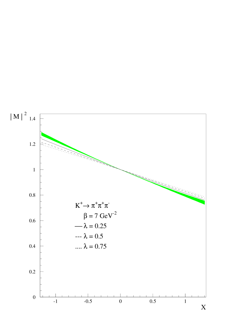
Figure 3:

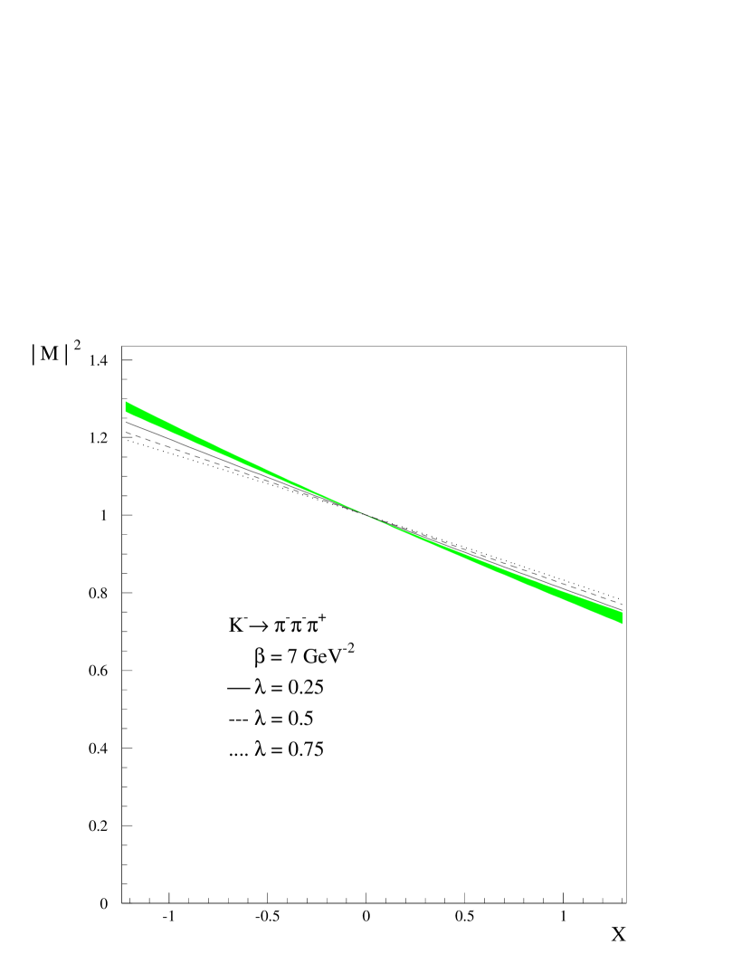
Figure 4:

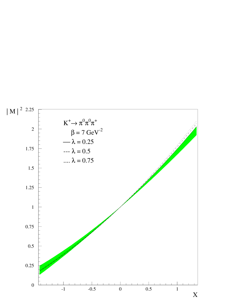
Figure 5:

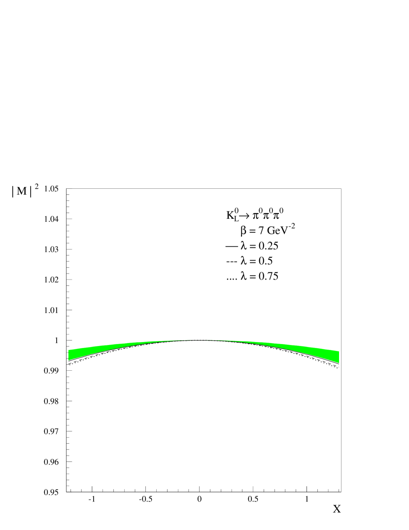
Figure 6:

References

- [1] S. Weinberg, Phys. Rev. Lett. 4 (1960)87
-
[2]
Particle Data Group, Review of Particle Physics;
Eur. Phys. J. C15 (2000)1 -
[3]
S. Somalwar et al., Phys. Rev. Lett. 68
(1992)2580
NA48 Collaboration (A. Lai et al.), Phys.Lett., B515 (2001)261 - [4] V. Y. Batusov et al., Nucl. Phys. B516 (1998)3
-
[5]
J. Kambor, J. Missimer and D. Wyler, Phys. Lett.
B261 (1991)496
J. Kambor, et al. Phys. Rev. Lett. 68 (1992)1818
A. Belkov, et al. Int. J. Mod. Phys. A7 (1992)4757
G. D’Ambrosio, et al. Phys. Rev. D50 (1994)5767 -
[6]
Goldhaber G., Goldhaber S., Lee W., Pais A.,
Phys. Rev. 120 (1960)300 - [7] E. Cuautle, G. Herrera, Phys. Lett. B434 (1998)153
- [8] G.D. Lafferty, Z. Phys. C60 (1993)659
- [9] A. Bialas and A. Krzywicki, Phys. Lett. B354 (1995)134
- [10] L. Lonnblad and T. Sjostrand, Phys. Lett. B351 (1995)293
- [11] Phuong Mai Dinh, Nicolas Borghini, Jean-Yves Ollitrault Phys. Lett. B477 (2000)51
- [12] S.R. Amendolia et al., Phys. Lett.B178 (1986)435
-
[13]
R. Hernández and G. Herrera, Phys. Lett. B332
(1994)448
A. Gago and G. Herrera, Mod. Phys. Lett. A10(1995)1435 - [14] D.H.Boal, C.K.Gelbke, B.K.Jennings, Rev. Mod. Phys. 62 (1990)553
- [15] M.I. Martinez and G. Herrera, in preparation
- [16] W. T. Ford et al., Phys. Lett. 38B(1972)335