Light-cone representation of the quark Schwinger-Dyson equation.

Abstract

We use a light-cone approach to solve the Schwinger-Dyson equation for the quark propagator. We show how this method can be used to solve the equation beyond the space-like region, to which one is usually restricted with the Euclidean-space approach. We work in the Landau gauge, and use an infrared-enhanced model for the gluon propagator and include instanton effects to get both confinement and vacuum condensates. With our models reasonable fits to known quantities are obtained, resulting in a light-cone quark propagator that can be used for hadronic physics at all momentum transfers.

I Introduction.

For a microscopic QCD description of hadrons and hadronic matter one needs the fully dressed nonperturbative quark and gluon propagators, for which the Schwinger-Dyson formalism is a natural approach. A full study of QCD, however, requires investigation of hadronic properties at all momentum transfers. Since instant form of field theory is difficult to use for composite states at medium or high momentum, a light-cone representation is desirable[1]. In the present paper we develop a light-cone formulation of the Schwinger-Dyson equation for the quark propagator for use in developing hadronic light-cone Bethe-Salpeter amplitudes as well as providing new aspects of the quark propagator, which we discuss below.

It is well known that short distance processes occurring inside hadrons are well described by perturbative QCD (p-QCD) calculations. It is also well known that quarks never emerge as such from the reaction region, but instead they hadronize at a distance of about a fermi. But often these processes are not well described by p-QCD. The reason is that perturbative calculations in QCD have a rather limited range of validity: they are a good approximation only at very short distances where the expansion parameter (the effective QCD coupling constant) is small. But if QCD is the correct theory of the strong interactions (and that is the consensus today), then it should describe medium and long distance hadronic processes as well. We need then to understand how to compute the basic entities of the theory (its Green’s functions) not just over very short distances, but over long distances too.

The Schwinger-Dyson equations of a field theory embody all its dynamics [2, p. 475]. They are the complete equations of motion for the Green’s functions of the theory, and thus provide a natural way for studying the theory beyond the limited scope of perturbative expansions. Unfortunately they consist of an infinite tower of coupled integral equations relating full $n$-point functions to full $(n+1)$-point functions. Thus, the integral equation satisfied by one propagator may involve another propagator and a three-point vertex. The equation for this vertex may in turn include another propagator and a four-point vertex or scattering kernel, and so on. Some physically motivated truncation scheme becomes mandatory before the infinite tower can be brought to a manageable size. As it has been stressed in [3] the Ward identities of gauge theories significantly ease this truncation, since they imply that two-point functions (propagators) uniquely determine the longitudinal part of three-point functions (vertices).

The Schwinger-Dyson equation for the fermion and gauge boson propagators in QCD and QED have been studied using different approximations and models. For an excellent review see [4] and references therein. A recurring topic in this area is the question of the analytic structure of the propagators. For the electron propagator one expects a singularity at $p^{2}=m_{phys}^{2}$. For a confined particle like the quark it is not so clear what one should expect, it depends on what the confining mechanism is. Coleman  [5, pp. 378-386] has shown that it is perfectly possible for a confined particle to have a pole in its propagator at a positive real (i.e., physical and time-like) value of $p^{2}$.

Fermion propagators with branch points at complex conjugate locations off the real axis of the variable $p^{2}$, have been obtained since more than twenty years ago for QED [6], and more recently for QCD as well [4]. This has been studied in great detail by Maris [7]. In the case of QED, where we know that there must be a singularity at $p^{2}=m_{phys}^{2}$, this is thought to be an artefact of the approximations with no physical significance. For QCD, the absence of singularities on the real axis has been thought to be related to quark confinement. Şavkli and Tabakin [8] have shown that the imaginary part of the value of $p^{2}$ where the singularity occurs may be interpreted as a decay width for a single quark state, and can be related to the hadronization distance. However, the fact that in two physical situations as different as those of QED and QCD the singularities seem to have the same origin [7] makes any physical interpretation difficult. The location of these singularities poses yet another difficulty: it invalidates the Wick rotation, and thus makes the theory as defined in Euclidean metric not equivalent to that defined in Minkowski metric.

In this paper we study the Schwinger-Dyson equation for the quark propagator starting from its Minkowski-space formulation. We do make assumptions about the location of the singularities similar to those necessary to justify a Wick rotation. However, we arrive at a formulation that allows us to solve for the quark propagator in the space-like region (which would correspond to a solution in Euclidean space) or, in principle, to extend into the time-like region as far as needed.

Our derivation of the Schwinger-Dyson equation in a light-cone representation is discussed in detail in section II. The method is an extension of the method used in perturbation theory [9] to obtain an infinite momentum frame formulation, which in many respects is equivalent to the light-cone field theory formulation of perturbative diagrams. It is also analogous to the method for obtaining a light-cone representation of the Bethe-Salpeter equation from the standard four- dimensional instant-form, however, as explained in section II the simple prescription for projecting onto the light cone cannot in general be used for the SD equation.

In section III we discuss our models. In sections IV and V we discuss some technical aspects of solving the equations and give sample results in Minkowski space. In section VI we discuss the results of our model calculations and in section VII give our conclusions.

II The quark SD Equation and the light-cone.

In this section we discuss our light-cone formulation the Schwinger-Dyson equation. Since the light-cone representation of the Bethe-Salpeter (BS) equation for bound systems is described extensively in the literature, we also briefly review the BS equation to motivate the present work and explain its applicability.

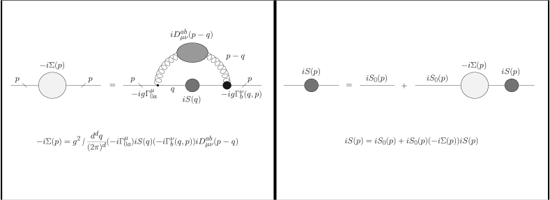
FIG. 1.: Diagrammatic representation of the Schwinger-Dyson equation for the quark propagator.

The full dressed quark propagator satisfies the Schwinger-Dyson (SD) equation (see Fig 1):

$$S^{-1}(p) = S_{0}^{-1}(p)-\raisebox{-2.15277pt}{\mbox{$\Sigma$}}(p)$$ (1)

$$\raisebox{-2.15277pt}{\mbox{$\Sigma$}}(p) = ig^{2}\int\frac{d^{d}q}{(2\pi)^{d}}\Gamma^{\mu}_{0a}S(q)\Gamma^{\nu}_{b}(q,p)D^{ab}_{\mu\nu}(p-q),$$ (3)

where $\Gamma^{\nu}_{b}(q,p)$ and $D^{ab}_{\mu\nu}(p-q)$ are the dressed quark-gluon vertex and dressed gluon propagator. Greek letters represent Lorentz indices and Latin letters stand for color indices. The color structure of all quantities in (LABEL:original) is known:

  

The bare vertex: $\Gamma^{\mu}_{0a}=\gamma^{\mu}\lambda_{a}/2$

  

The dressed vertex: $\Gamma^{\nu}_{b}(q,p)=\Gamma^{\nu}(q,p)\lambda_{b}/2$

  

The gluon propagator: $D^{ab}_{\mu\nu}(k)=\delta^{ab}D_{\mu\nu}(k)$

so that the color indices can be contracted: $\lambda_{a}\lambda_{b}\delta^{ab}=16.$ The inverse bare propagator is $S_{0}^{-1}(p)=\not\!{p}-m_{c}$ , with the current quark mass $m_{c}$ zero in the chiral limit or estimated from PCAC.

The solutions of the Schwinger-Dyson equation are of the form

$$S^{-1}(p)=A(p^{2})\not\!{p}-B(p^{2}).$$ (4)

Physically, the most significant aspect of the solution for the two functions $A(p^{2})$ and $B(p^{2})$ is the ratio $M(p^{2})=B(p^{2})/A(p^{2})$, which is interpreted as the effective mass of the dressed quark propagator. Since isolated quarks are confined, the interpretation of this mass is not straight-forward as for the electron SD equation.

The light-cone formulation of quantum mechanics[1] starts with the demonstration that in the light-cone representation one obtains light-cone Poincare generators, with an interaction-free Lorentz boost in one direction. One can also show that the analogous result is true in a light-cone field theory. This enables one to study high momentum transfer processes, such as form factors in the region above 1 GeV, which is very difficult in the instant form. Although there was work on the SD equation three decades ago for perturbative QED [9], for nonperturbative QCD the problem is quite different, as we show below. Before discussing the light-cone representation of the Schwinger-Dyson equation we review the well-known light-cone representation of the Bethe-Salpeter equation. Since in physical application of the BS amplitudes to form factors and transition amplitudes one needs the dressed quark propagator, the main motivation of our present work is to formulate a light-cone Schwinger-Dyson (LCSD) equation to be used with the light-cone Bethe-Salpeter (LCBS) formalism.

There has been a great deal of work on bound state problems in light-cone representations based on the Bethe-Salpeter (BS) equation. For example, the BS equation for the pion in relative coordinates has the form

$$\Psi(k)=\int d^{4}l{\cal K}(k,l)\Psi(l),$$ (5)

where ${\cal K}$ is the kernel and $\Psi$ is the BS amplitude. One can obtain a light-cone representation [10] by inserting a delta function to include the light-cone on-shell condition and eliminate the $l^{-}$ variable

$$\Psi(x,{\bf k}_{\perp}) = \int[dy][d^{2}{\bf l}_{\perp}]{\cal K}(x,{\bf k}_{\perp};y,{\bf l}_{\perp})\Psi(y,{\bf l}_{\perp}).$$ (6)

BS amplitudes from this type of equation have been used to study the transition from nonperturbative to perturbative regions [11, 12]. We emphasize that for such calculations both on-shell and off-shell aspects of the SD functions $A(p^{2}),B(p^{2})$ are needed. Therefore the prescription of projecting onto the light cone as for the BS equation is not appropriate.. We now discuss our approach to the the SD equation for the quark propagator on the light cone.

We solve equation (LABEL:original) in a light-cone representation by using a method introduced originally for perturbation theory. In Ref  [9] S.Chang and S. Ma showed how the rules of light-cone perturbation theory (LCPT)  can be derived from the usual covariant Feynman rules simply by changing into light-cone variables:

$\displaystyle q^{\pm}=q^{0}\pm q^{3},\;\;{\bf q}_{\perp}=\left(q^{1},q^{2}\right)$

In simple calculations, like a one-loop self-energy diagram, an important feature of the new rules becomes apparent: the range of integration over the $q^{+}$ variable becomes finite

$\displaystyle\int_{-\infty}^{+\infty}dq^{+}\longrightarrow\int_{0}^{p^{+}}dq^{+},$

where $p^{+}$ is the “plus” (longitudinal) component of the external momentum. As shown in that paper, this feature is related to the fact that in LCPT there are no diagrams with lines going backwards in time and no vacuum diagrams (with the exception of zero modes and instantaneous terms in fermion propagators). This is a crucial property of light-cone field theory, since it simplifies tremendously the structure of the vacuum.

In solving the Schwinger-Dyson equation we are faced with the non-perturbative self-energy diagram seen in Fig. 1:

$$\int\frac{d^{d}q}{(2\pi)^{d}}q^{\mu_{1}}q^{\mu_{2}}\ldots q^{\mu_{n}}f_{Q}\left(q^{2}+i\epsilon\right)f_{G}\left((p-q)^{2}+i\epsilon\right)$$ (7)

Consider first the scalar case $n=0$. Using the variables:

$\displaystyle\alpha=q^{+}/p^{+},\;\;s^{\prime}=q\cdot q,\;\;s=p\cdot p,\;\;{\bf q^{\prime}}_{\perp}={\bf q}_{\perp}-\alpha\;{\bf p}_{\perp},$

the integral in (7) becomes:

$$\int\frac{ds^{\prime}d\alpha d^{d-2}{\bf q^{\prime}}_{\perp}}{2|\alpha|(2\pi)^{d}}f_{Q}\left(s^{\prime}+i\epsilon\right)f_{G}\left(-\alpha^{-1}{\mathcal{P}}(q^{{}^{\prime}2}_{\perp},s,s^{\prime},\alpha,\epsilon)\right),$$ (8)

where all the integrals are from minus infinity to plus infinity, and

$\displaystyle{\mathcal{P}}(q^{{}^{\prime}2}_{\perp},s,s^{\prime},\alpha,\epsilon)\equiv q^{{}^{\prime}2}_{\perp}+\alpha(1-\alpha)(-s)+(1-\alpha)s^{\prime}-i\alpha\epsilon$

is reminiscent of the similar quantity that appears after the well known Feynman trick of combining denominators. Particularly, if $s^{\prime}=m^{2}_{0}-i\epsilon$ and $f_{G}(s)=1/(s-m^{2}_{1})^{a_{1}}$, then after the ${\bf q^{\prime}}_{\perp}-$integration

$\displaystyle\alpha^{-1}f_{G}\left(-\alpha^{-1}{\mathcal{P}}\right)\rightarrow\frac{(-1)^{-a_{1}}\alpha^{a_{1}-1}}{\left(\alpha(1-\alpha)(-s)+(1-\alpha)m^{2}_{0}+\alpha m^{2}_{1}-i\epsilon\right)^{a_{1}}},$

a very familiar expression.

Returning to (8), let now $s^{\prime}_{Q}$ and $s^{\prime}_{G}$ be singular points of $f_{Q}$ and $f_{G}$, respectively. Then the integrand in (8) has singularities at values $s^{\prime}=s^{\prime}_{1}$ and $s^{\prime}=s^{\prime}_{2}$ with imaginary parts given by:

$\displaystyle Im\left(s^{\prime}_{1}\right)=Im\left(s^{\prime}_{Q}\right)-\epsilon,\mbox{ and }Im\left(s^{\prime}_{2}\right)=\frac{\alpha}{\alpha-1}\left[Im\left(s^{\prime}_{G}\right)-\epsilon\right].$

It is then clear that if both $s^{\prime}_{Q}$ and $s^{\prime}_{G}$ are on or below the real axis, then the corresponding singularities of the integrand will be on opposite sides of the real axis iff $\alpha/\left(\alpha-1\right)<0$, i.e., $0<\alpha<1$. For values of $\alpha$ outside this interval, both singularities fall on the same side of the real axis, and the contour of the $s^{\prime}$ integration can be closed with a semicircle that doesn’t contain either of them. Thus if all the singularities of the functions $f_{Q}$ and $f_{G}$ occur on or below the real axis, only the interval $(0,1)$ in the integration over $\alpha$ contributes to the integral . This reasoning is only a slight modification of that presented in [9]. The integral in (8) then becomes

$$\frac{1}{4\pi}\int_{-\infty}^{+\infty}\frac{ds^{\prime}}{2\pi}\!\int_{0}^{1}\!d\alpha\!\int\frac{d^{d-2}{\bf q^{\prime}}_{\perp}}{(2\pi)^{d-2}}\alpha^{-1}f_{Q}\left(s^{\prime}+i\epsilon\right)f_{G}\left(-\alpha^{-1}{\mathcal{P}}(q^{{}^{\prime}2}_{\perp},s,s^{\prime},\alpha,\epsilon)\right).$$ (9)

In dealing with fermion propagators we encounter integrals with powers of the momenta in the numerator as shown in (7). As discussed in [9], in such cases the previous reasoning fails for some components of the integrals (usually referred to as “bad” components). The issue then arises as to whether or not one can avoid all such components. In all such cases we are able to avoid them and compute only the “good” components. The “bad” components are recovered by the requirements of Lorentz symmetry.

We see that to preserve the rules of light-cone theory we must make assumptions about the location of the singularities, much like those necessary to justify a Wick rotation.

A comment on (9) as compared to a typical calculation of a perturbative diagram in a light-cone approach is in order. In most light-cone calculations, the integral over $q^{-}$ (equivalent to the integral over $s^{\prime}$ in (9)) is absent. An on-shell condition that determines the value of $q^{-}$ is used, instead of integrating over all values. In other words, the calculations are performed in time-ordered perturbation theory (TOPT). This has become so customary that the rules of light-cone TOPT are often identified with the rules of light-cone theory. The equivalence between TOPT (either light-cone or equal-time) and the Feynman rules is usually shown by closing a contour of integration to pick up a singularity in a propagator and thus put a particle on shell. This can be done in the equal-time formulation (by doing first the integral over $q^{0}$, for example) or in light-cone formulation (by doing first the integral over $q^{-}$). One should refrain from doing so in dealing with the Schwinger-Dyson equation. Most certainly, the singularities of the Green’s functions involved are more complicated than just a pole, for one thing: this is not perturbation theory. While such practice comes in naturally in the equal-time formulation, where TOPT is not very customary, it raises a flag in a light-cone approach. Hopefully, this comment addresses that flag.

III Models

There has been an extensive program of research on the Schwinger-Dyson equation during the past decade. See [4, 13] for reviews. The usual approach is to model the gluon propagator and to use symmetries to express the dressed vertex in terms of the propagators, or to use the free vertex. The model is constrained by the vacuum condensates. We follow this general procedure in our light-cone approach. Since our approach allows one to define meson form factors for all momentum transfers, which is not true of instant-form approaches, applications of our solutions to hadronic properties will be most interesting.

The Lorentz tensor structure of the gluon propagator has the general form:

$$D_{\mu\nu}(k)=\frac{-1}{k^{2}+i\epsilon}\left\{\left(g_{\mu\nu}-\frac{k_{\mu}k_{\nu}}{k^{2}+i\epsilon}\right)D(k^{2})+\xi\frac{k_{\mu}k_{\nu}}{k^{2}+i\epsilon}\right\}$$ (10)

here $\xi$ is the gauge parameter. The choice of a model is to pick a value of $\xi$, such as $\xi=0$ for the Landau gauge and the form of the function D($k^{2}$). The two essential nonperturbative features that the gluon propagator must be consistent with are confinement and the vacuum condensates. It has long been known that with the gluon propagator having a $1/k^{4}$ behavior there is confinement[14] and one can fit the string tension. On the other hand, it is also known that with the instanton liquid model [15] one can fit the quark and gluon condensates. The two models that we investigate in the present work are the polynomial model and the instanton model, motivated by these two features of nonperturbative QCD.

A Polynomial model

We work in Landau gauge with $\xi=0$, and take as our model gluon propagator

$$D_{\mu\nu}(k)=\frac{-1}{k^{2}+i\epsilon}\left(g_{\mu\nu}-\chi\frac{k_{\mu}k_{\nu}}{k^{2}+i\epsilon}\right)D(k^{2}),$$ (11)

with the parameter $\chi$ introduced to allow us to use a Feynman-like gauge (the gauge where $D_{\mu\nu}(k)\propto g_{\mu\nu}$). Thus $\chi=0$ for Feynman-like gauge and $\chi=1$ for Landau gauge. See Refs[4, 13] for discussions the choice of gauge and gauge invariance for Schwinger-Dyson equation in QCD.

It has been shown elsewhere [16] that renormalization group arguments yield an approximate relation between the renormalized coupling constant, the renormalized gluon propagator and the effective coupling:

$$g^{2}_{R}D_{R}(k^{2})\approx g_{eff}^{2}(k^{2})=4\pi\alpha_{eff}(k^{2}),$$ (12)

where the subscript $R$ denotes renormalized quantities, and $g_{eff}$ is the effective running coupling constant. The renormalized coupling is related to the running coupling by $g^{2}_{R}\equiv\left.g^{2}_{eff}(Q^{2})\right|_{Q^{2}=\mu^{2}}$, where $\mu^{2}$ is the renormalization point.

As discussed in  [4, section 6.1], Eq.(12), and the fact that in Landau gauge only the combination $g^{2}D\left(k^{2}\right)$ enters the Schwinger-Dyson equation, reduces the problem of modeling the non-perturbative part of the gluon propagator to that of modeling the non-perturbative part of $\alpha_{eff}$. We model $\alpha_{eff}$ with the expression:

$$\alpha_{eff}(k^{2})=\sum_{l=1}^{N}(-1)^{c_{l}}\lambda_{l}\left(\frac{s_{0}}{k^{2}+i\epsilon}\right)^{c_{l}}.$$ (13)

Although the known logarithmic behavior of $\alpha_{eff}$ in the high energy limit cannot be fitted accurately with this form, a reasonable approximation can be obtained up to energies well beyond our main region of interest. Thus, for example, with $N=2,\;s_{0}=1\mbox{ GeV}^{2},\;\lambda_{1}=0.222,\;c_{1}=0.07,\;\lambda_{2}=0.25,\;c_{2}=0.6$ the values for $\alpha_{eff}$ obtained from our fit are within the accepted error bars as published, for example, by PDG[17] for energies from about 1.3 GeV to 350 GeV [see Fig 2]. Fits good to higher energies can always be achieved by adding more terms in (13) with smaller $c_{l}$. As can be seen in Fig. 2, with these parameters, our model underestimates the accepted values for $\alpha_{eff}$ in the important energy range of a few hundred MeV to about 1.2 GeV, although it is widely believed that it overestimates them in the deep infrared.

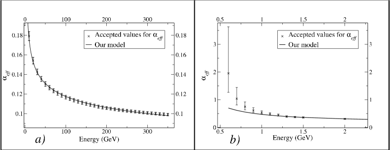
FIG. 2.: Fitting $\alpha_{eff}$ with Eq.(13). See text for values of parameters. a) For energies up to 350 GeV. b) A close-up for lower energies.

There is little certainty about what happens to the effective coupling or the gluon propagator at very low energies. Some results [18, 16] suggest that the pole at $k^{2}=0$ gets enhanced and could be as strong as $1/k^{4}$. This would provide an explanation for confinement as shown by ’tHooft [14]. Other results [19, 20] suggest that the pole gets softer or disappears and that the gluon picks up an effective mass. Our model describes an infrared-enhanced gluon propagator, although not as strongly as $1/k^{4}$.

B Instanton model

As we shall discuss in section VI below, one cannot obtain the known quark condensates with the polynomial model. On the other hand, it is known that with a pure instanton model one can obtain the quark condensate but not the string tension. For this reason we consider a model with quarks propagating in the instanton medium and in addition the gluon propagator having a 1/$k^{\alpha}$ structure to get confining effects of the far infrared. The starting point is the solution for the instanton using the classical action [24], which gives for the instanton color field

$$A^{inst}_{\mu(x)a} = \frac{2\eta_{a\mu\nu}x_{\nu}}{x^{2}+\rho^{2}}$$ (14)

$$G^{inst}(x)\cdot G^{inst}(x) = \frac{192\rho^{4}}{(x^{2}+\rho^{2})^{4}}$$ (15)

where $\rho$ is the instanton size. The quark zero modes in the instanton background [25], for the + mode with the instanton at position $z$, are

$$\Psi_{z}(x) = \frac{\rho}{\sqrt{x^{2}}\pi(x^{2}+\rho^{2})^{3/2}}\frac{1+\gamma_{5}}{2}\gamma_{\alpha}(x_{\alpha}-z_{\alpha})U,$$ (16)

where $\rho$ is the instanton size and $U$ is a unitary color-spin matrix. From this the widely used model of the quark propagating in the instanton-antiinstanton medium[26] was derived.

$$A_{I}(p)-1 = 0$$ (17)

$$B_{I}(p) = Kp^{2}f^{2}(\frac{5}{6}p)$$ (18)

$$f(p) = \frac{2}{p}-(3I_{0}(p)+I_{2}(p))\times K_{1}(p).$$ (19)

The quark propagating in the instanton-antiinstanton medium is illustrated in Fig. 3.

FIG. 3.: Quark propagating in instanton medium

In our model with instantons we include this propagator in the Schwinger-Dyson equation by adding it to the free propagator. The justification for this model is that the instantons give the nonperturbative QCD at the length scale of about 1/3 fm, while the polynomial model gives the far infrared behavior. As a simple example of the physics missing if one uses only the polynomial model for the gluon propagator and ignores instanton effects consider a delta-function model for the gluon propagator. See, e.g., Ref.[13] for the solutions to the Schwinger-Dyson equation in such a model. The quark and mixed quark condensates are given by

$$\langle 0|:\bar{q}(0)q(0):|0\rangle=-\frac{3}{4\pi^{2}}\int_{0}^{+\infty}dSS\frac{B(S)}{SA^{2}(S)+B^{2}(S)}$$ (20)

$$\langle 0|:\bar{q}(0)g\sigma\cdot G(0)q(0):|0\rangle=$$ (22)

$$\frac{9}{4\pi^{2}}\int_{0}^{+\infty}dSS\left\{S\frac{B(S)(2-A(S))}{SA^{2}(S)+B^{2}(S)}+\frac{81B(S)[2SA(S)(A(S)-1)+B^{2}(S)]}{16(SA^{2}(S)+B^{2}(S))}\right\}.$$ (24)

One can fit the strength of the delta function gluon propagator to obtain the correct quark condensate. Then from Eqs. (20) it is simple to calculate the mixed quark condensate. The result is an order of magnitude different from the phenomenological value. This is an example of the need to include both the long-distance and the medium-distance nonperturbative QCD effects. We return to this when we discuss the results of our calculations. For completeness we include here the equation for $f_{\pi}$  [4, Appendix C]

$\displaystyle f^{2}_{\pi}=\frac{3}{4\pi^{2}}\int^{+\infty}_{0}dS\frac{SM(S)}{A(S)[S+M^{2}(S)]^{2}}\left[M(S)-\frac{S}{2}\frac{dM}{dS}\right].$

Notice that in these equations $S$ denotes Euclidean momentum.

C The vertex

The results reported in this paper were all obtained with the approximation $\Gamma_{\mu}(p,q)=\gamma_{\mu}$ (rainbow approximation). The popularity of this approximation is justified by its simplicity. It suffers the serious drawback of violating the Ward-Takahashi identity (WTI):

$$(p-q)^{\mu}\Gamma_{\mu}(p,q)=S^{-1}(p)-S^{-1}(q)$$ (25)

This identity holds in QED, and the forms for the vertex discussed below were proposed for QED. Such forms are, however, often used for QCD as well, since the analogous identity for QCD (known as the Slavnov-Taylor identity) reduces to (25) if ghost effects are ignored. Ignoring these effects is believed to be important in the infrared region.

This identity can be used to express the longitudinal part of the vertex in terms of the propagator. Ball and Chiu [21] have proposed the form:

$$\Gamma_{\mu}(p,q)=\Gamma_{\mu}^{BC}(p,q)+\sum_{i-1}^{8}f^{i}\left(p^{2},q^{2},p\cdot q\right)T^{i}_{\mu}(p,q),$$ (26)

where the $T_{\mu}^{i}$’s are eight transverse tensors (i.e. tensors that satisfy $(p-q)^{\mu}T^{i}_{\mu}(p,q)=0$, and thus don’t contribute to the WTI). The form of these tensors is given in Eq.(3.4) of [21]. The eight scalar functions $f^{i}$ are not constrained by the WTI. $\Gamma^{BC}_{\mu}$ is given by:

$$\Gamma^{BC}_{\mu}(q,p)=\gamma_{\mu}\left(A(q^{2})(1-\beta_{1})+A(p^{2})\beta_{1}\right)+$$ (27)

$${\displaystyle+(q+p)_{\mu}\left(\not\!{q}\beta_{1}+\not\!{p}(1-\beta_{1})\right)\frac{A(q^{2})-A(p^{2})}{q^{2}-p^{2}}-(q+p)_{\mu}\frac{B(q^{2})-B(p^{2})}{q^{2}-p^{2}}}.$$ (29)

This is really a small modification of the vertex proposed by Ball and Chiu. In their form $\beta_{1}=1/2$, but other values are often used to explore the effects of the transverse part. Besides compromising the symmetry of $\Gamma_{\mu}$, changing the value of $\beta_{1}$ can have serious effects on renormalizability, namely because of its effect on the transverse part, as discussed below. The WTI itself is satisfied for any value of $\beta_{1}$, and for any choice of $f^{i}$’s. The converse is also true: any vertex that satisfies the WTI can be expressed through (26, 27).

The vertex has been further constrained by other studies, in particular, Burdens and Roberts [22] list a number of requirements $\Gamma_{\mu}$ should satisfy, besides the WTI. See also  [4, section 3.7]. Exploiting these requirements, and particularly the need to maintain multiplicative renormalizability in QED, Curtis and Pennington [23] narrowed down the last term in Eq.(26) to:

$$\Gamma^{CP}_{\mu}(q,p)=\beta_{2}\left(\gamma_{\mu}(q^{2}-p^{2})-(q+p)_{\mu}(\not\!{q}-\not\!{p})\right)\frac{(q^{2}+p^{2})\left(A(q^{2})-A(p^{2})\right)}{(q^{2}-p^{2})^{2}+\left(M^{2}(q^{2})+M^{2}(p^{2})\right)^{2}}.$$ (30)

Here too $\beta_{2}=1/2$ in the original formulation. Applying the approach explained in section II, we have found that when using

$\displaystyle\Gamma_{\mu}(q,p)=\Gamma^{BC}_{\mu}(q,p)+\Gamma^{CP}_{\mu}(q,p),$

one must set consistently $\beta_{1}=\beta_{2}$. This ensures, for example that the function $A$ remains free of divergencies in Landau gauge, a well established result. Notice that this implies that using $\Gamma^{BC}_{\mu}$ by itself is, in general, inconsistent.

We are currently investigating using this form in our model. Although that entails neglecting the effect of ghost fields in the STI, it is a significant improvement over the rainbow approximation.

IV Integrating the equations.

In order to solve (LABEL:original) in our model, we need to calculate integrals of the type (here $a_{l}=1+c_{l}$):

$$\displaystyle\lim_{\epsilon\to 0^{+}}\int\frac{d^{d}q}{(2\pi)^{d}}\frac{f_{Q}(q^{2}+i\epsilon)}{\left((p-q)^{2}-m^{2}_{1}+i\epsilon\right)^{a_{l}}}\left\{1,\>q^{\mu},\>q^{\mu}\,q^{\nu}\right\}\equiv$$ (31)

$$\mbox{}\left\{C_{00}(p^{2};f_{Q},a_{l}),p^{\mu}C_{10}(p^{2};f_{Q},a_{l}),p^{\mu}p^{\nu}C_{20}(p^{2};f_{Q},a_{l})+g^{\mu\nu}C_{01}(p^{2};f_{Q},a_{l})\right\},$$ (33)

where we have exploited the Lorentz structure to define the scalar quantities $C_{rj}$.

These integrals include as a particular case the well known integrals:

$$\displaystyle\lim_{\epsilon\to 0^{+}}\int\frac{d^{d}q}{(2\pi)^{d}}\frac{\left\{1,\>q^{\mu},\>q^{\mu}\,q^{\nu}\right\}}{\left(q^{2}-m^{2}_{0}+i\epsilon\right)^{a_{0}}\left((p-q)^{2}-m^{2}_{1}+i\epsilon\right)^{a_{l}}}\equiv$$ (34)

$$\mbox{}\left\{I_{00}(p^{2};a_{0},a_{l}),p^{\mu}I_{10}(p^{2};a_{0},a_{l}),p^{\mu}p^{\nu}I_{20}(p^{2};a_{0},a_{l})+g^{\mu\nu}I_{01}(p^{2};a_{0},a_{l})\right\}.$$ (36)

For $(r,j)=(0,0),(1,0),(2,0),(0,1)$, the $I^{\prime}s$ are known to be:

$$I_{rj}(s;a_{0},a_{l})=\frac{i(-1)^{-(a_{0}+a_{l})}(-1/2)^{j}}{(4\pi)^{d/2}}\Gamma\left[\begin{array}[]{c}a_{0}+a_{l}-d/2-j\\ a_{0},a_{l}\end{array}\right]\times$$ (39)

$$\displaystyle\int_{0}^{1}d\alpha\frac{\alpha^{a_{l}+r-1}(1-\alpha)^{a_{0}-1}}{(\alpha(1-\alpha)(-s)+(1-\alpha)m_{0}^{2}+\alpha m_{1}^{2}-i\epsilon)^{a_{0}+a_{l}-d/2-j}},$$ (41)

where we have used the compact notation

$\displaystyle\Gamma\left[\begin{array}[]{c}a_{1},a_{2},\ldots,a_{n}\\ b_{1},b_{2},\ldots,b_{m}\end{array}\right]=\frac{\Gamma(a_{1})\Gamma(a_{2})\ldots\Gamma(a_{n})}{\Gamma(b_{1})\Gamma(b_{2})\ldots\Gamma(b_{m})}\;.$

For the $C^{\prime}s$, we proceed as explained in section II to get:

$$\mbox{}C_{rj}(s;f_{Q},a_{l})=\frac{i(-1)^{-a_{l}}(-1/2)^{j}}{(4\pi)^{d/2}}\Gamma\left[\begin{array}[]{c}a_{l}+1-d/2-j\\ a_{l}\end{array}\right]\int_{-\infty}^{+\infty}\frac{f_{Q}(s^{\prime}+i\epsilon)ds^{\prime}}{2\pi i}$$ (44)

$$\displaystyle\int_{0}^{1}d\alpha\frac{\alpha^{a_{l}+r-1}}{(\alpha(1-\alpha)(-s)+(1-\alpha)s^{\prime}+\alpha(m_{1}^{2}-i\epsilon))^{a_{l}+1-d/2-j}}.$$ (46)

At this point we must make sure that if we set $f_{Q}\left(s^{\prime}\right)=1/\left(s^{\prime}-m^{2}_{0}\right)^{a_{0}}$, then (44) agrees with (39). This is most easily done by closing the contour of integration of the $s^{\prime}$ variable with an infinite semicircle in the lower half of the complex plane to pick up the singularity  in $f_{Q}$. This procedure, however, uses the analytic form of $f_{Q}$. We need a procedure that would rely only on the numerical values of $f_{Q}$. We perform the integrations by closing our contour with an infinite semicircle on the upper half of the complex plane to pick up the singularity (in $s^{\prime}$) of the expression on the second line of (44). For $m_{1}=0$, the $I^{\prime}s$ reduce to :

$$I_{rj}(s;a_{0},a_{l})=$$ (47)

$$\displaystyle\frac{i(-1)^{-(a_{0}+a_{l})}(-1/2)^{j}}{(4\pi)^{d/2}(m_{0}^{2})^{a_{0}+a_{l}-d/2-j}}\Gamma\left[\begin{array}[]{c}a_{0}+a_{l}-d/2-j,a_{l}+r,d/2+j-a_{l}\\ a_{0},a_{l},d/2+j+r\end{array}\right]$$ (51)

$$\displaystyle{}_{2}F_{1}(a_{0}+a_{l}-d/2-j,a_{l}+r;d/2+j+r;s/m_{0}^{2}).$$ (53)

For the $C^{\prime}s$:

$$C_{rj}(s;f_{Q},a_{l})=-\frac{i(-1)^{-a_{l}}(-1/2)^{j}}{(4\pi)^{d/2}\Gamma[a_{l}]}\times$$ (54)

$$\left\{\begin{array}[]{l@{\hspace{-20mm}}r}{\displaystyle\Gamma\left[\begin{array}[]{c}b\\ 1+b-a\end{array}\right](-s)^{-b}\int_{0}^{s}ds^{\prime}f_{Q}(s^{\prime})(-s^{\prime})^{b-a}{}_{2}F_{1}(1+b-c,b;1+b-a;s^{\prime}/s)+}&\\ &\\ {\displaystyle+\Gamma\left[\begin{array}[]{c}b,c-b\\ c,1-a\end{array}\right]\int_{s}^{-\infty}ds^{\prime}f_{Q}(s^{\prime})(-s^{\prime})^{-a}{}_{2}F_{1}(a,b;c;s/s^{\prime})}&s<0\\ &\\ &\\ {\displaystyle\Gamma\left[\begin{array}[]{c}b,c-b\\ c,1-a\end{array}\right]\int_{0}^{-\infty}ds^{\prime}f_{Q}(s^{\prime})(-s^{\prime})^{-a}}&s=0\\ &\\ &\\ {\displaystyle\Gamma\left[\begin{array}[]{c}c-b\\ 1+c-a-b\end{array}\right]s^{1-c}\int_{s}^{0}ds^{\prime}f_{Q}(s^{\prime})(s-s^{\prime})^{c-a-b}(s^{\prime})^{b-1}{}_{2}F_{1}(1-a,1-b;1+c-a-b;1-s/s^{\prime})+}&\\ &\\ {\displaystyle+\Gamma\left[\begin{array}[]{c}b,c-b\\ c,1-a\end{array}\right]\int_{0}^{-\infty}ds^{\prime}f_{Q}(s^{\prime})(-s^{\prime})^{-a}{}_{2}F_{1}(a,b;c;s/s^{\prime})}&s>0,\end{array}\right.$$ (77)

where $a=a_{l}+1-d/2-j,\;b=a_{l}+r,\;c=d/2+j+r$.

V Sample calculations in Minkowski space.

In this section we discuss sample calculations in Minkowski space. The ability to work in Minkowski space is one of the important features of our light-cone formulation of the SD equation. in this section, however, we only use polynomial models, which allow convenient Minkowski space forms. As we shall see, the infra-red properties in these models are not consistent with the known condensates, and solutions with instanton contributions to the gluon propagator are much more satisfactory. Since the instanton forms have been obtained in Euclidean space, however, there is no unambiguous Minkowski space formulation. We discuss our results with models including instantons in the following section.

Eq.(54) is a generalization of the well known result Eq.(47) to a wider class of functions $f_{Q}$. The light-cone approach used, and in particular the treatment it makes of the singularities, seldom goes without some aftertaste. Here is a well known example where using light-cone variables leads to a dead end :

$\displaystyle\lim_{\epsilon\to 0^{+}}\int\frac{dk_{0}dk_{1}}{(k_{0}^{2}-k_{1}^{2}-m_{0}^{2}+i\epsilon)^{n}}\;\;\;n>1$

This integral is perfectly convergent and can be computed, for example, by closing the contour in the $k_{0}$-integration with a semicircle at infinity. The integral is, of course, non-vanishing. Using light-cone variables, one would have the integral:

$\displaystyle\lim_{\epsilon\to 0^{+}}\int\frac{dk^{+}dk^{-}}{2(k^{+}k^{-}-m_{0}^{2}+i\epsilon)^{n}}\;\;\;n>1$

If we now think of closing the contour of, say the $k^{-}$-integration, we see that the singularity occurs at $(m_{0}^{2}-i\epsilon)/k^{+}$. But then the singularity can always be avoided for any $k^{+}\neq 0$. Only for $k^{+}=0$ is the $k^{-}$-integration non-vanishing, but then, it must have a delta function type singularity.

The purpose of this section is test Eq.(54) against such anomalies, as well as to point out some important technicalities. We input a “first guess” for the quark propagator: $f_{Q}(s^{\prime})=1/(s^{\prime}-m_{0}^{2})$ with $m_{0}=2\mbox{ GeV}$, and use the model for the gluon propagator described in section III:

$\displaystyle g_{R}^{2}D_{R}(k^{2})=4\pi\left\{(-1)^{c_{1}}\lambda_{1}\left(\frac{s_{0}}{k^{2}+i\epsilon}\right)^{c_{1}}+(-1)^{c_{2}}\lambda_{2}\left(\frac{s_{0}}{k^{2}+i\epsilon}\right)^{c_{2}}\right\},$

where $s_{0}=1\mbox{ GeV}^{2},\;c_{1}=0.07,\;\lambda_{1}=0.222,\;c_{2}=0.6,\;\lambda_{2}=0.25$. We also discuss the ultravioletly divergent case $c_{1}=0$. For the vertex we set $\Gamma^{\nu}=\gamma^{\nu}$. We use Eq (54) to compute the functions $A\mbox{ and }B$ with this input. We exploit the fact that for the first iteration, the integrals could also be computed analytically using Eq.(47). We present graphs comparing the two outputs. We stress that these are not solutions to the Schwinger-Dyson equation but merely the output of running the iterative procedure once. Solutions to the Schwinger-Dyson equation are presented in section VI.

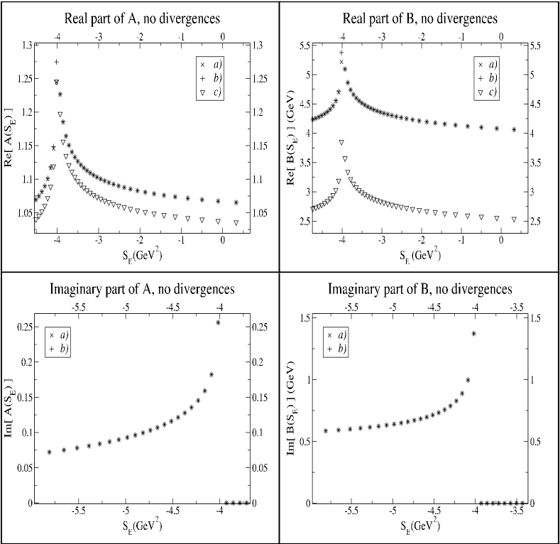
FIG. 4.: The quark propagator after one iteration compared with the analytic result. a) analytic result (47); numerical integrations of (54):b) with tail contribution, c) without tail contribution. Notice the appearance of a singularity and an imaginary part.

Keeping with tradition, the graphs are shown with a reversed x-axis. We use the variable $S_{E}\equiv-s$, equivalent to the Euclidean invariant momentum squared. We show, however, negative values of $S_{E}$, which lay outside the usual Euclidean space, and represent the time-like region. The numerical integration is carried out up to $S_{E_{MAX}}=64\mbox{ GeV}^{2}$ and an estimate of the contribution of the remaining integration out to infinity (“tail contribution”) is added. As will be seen on the graphs the consequences of omitting this tail contribution are numerically important.

In fact, in order to reproduce the numerical values of Eq.(47), Eq.(54) demands an elaborate integration procedure. On one hand there is the ever present fact of having to integrate over all energies. Renormalizability tells us that there is much freedom in dealing with the very high energy region (it can even be dropped, as in cut-off renormalization schemes), and whatever numerical effect that has on the integrals can be compensated by readjusting a finite number of parameters. From this point of view the effect of omitting the tail contribution, although numerically important, should be of no physical consequence. Eq.(47), however, represents the most accepted treatment of the very high energy regime: the integrals are carried out to infinity without the introduction of cut-offs or form factors that could spoil the symmetries of the theory. Divergencies, when they exist, are treated with the dimensional regularization method. In order to have Eq.(47) as a reference, we choose to carry out the integral in Eq.(54) out to infinity as well. In a numerical procedure this means adding an estimate of the tail contribution. On the other hand, we have a “floating singularity” in the integrand (a singularity at $S_{E}=S^{\prime}_{E}$, as opposed to one at a fixed point on the grid). This is particularly important for the infrared-enhanced terms (those with larger exponent $c_{l}$). Given the strength of the singularity at $S_{E}=S^{\prime}_{E}$, the contribution from the region $S_{E}\approx S^{\prime}_{E}$ is important. Sampling enough values of $S^{\prime}_{E}$ immediately to the left of $S_{E}$, is impossible when $S_{E}\approx S_{E_{MIN}}$, unless the grid is refined each time (the analogous problem around $S_{E_{MAX}}$ gets handled by the addition of the tail contribution). This can contribute to inaccuracies in the very low energy region, a most undesirable effect. Refining the grid with each iteration, however, can easily lead to exponential growth of the computational time.

FIG. 5.: The numerically renormalized quark propagator after one iteration in an ultraviolet divergent case, compared with the analytic $\overline{MS}$ result. a) analytic result (47); numerical integrations of (54): b) with tail contribution and $\overline{MS}$ subtraction, c) without tail contribution or $\overline{MS}$ subtraction.

One solution is to use a model propagator with no infrared enhancement, and that falls off rapidly at large energies, e.g., a Gaussian model. We don’t feel, however that Gaussian models are appropriate in the time-like region, and one of the purposes of this paper is to explore the effects of a tunable infrared enhancement. Our solution is to sample numerically only the part of the integrand involving the fermion propagator and the vertex, and to treat the part coming from the boson propagator (and containing the floating singularity) analytically. In the language of numerical methods, it is much along the lines of Gaussian quadratures. With this, and the addition of the tail contribution, the procedure becomes accurate, and reasonably fast.

The graphs in fig. 4 show the real and imaginary parts of the functions $A\mbox{ and }B$ after one iteration using the parameters above. As can be seen from the graphs, the procedure is quite accurate (provided the estimate of the tail contribution is added!). The relative error is of the order of thousandths of a percent, although it is somewhat larger right before (but not after!) the singularity at $S_{E}=-m_{0}^{2}$. The imaginary parts are obtained by simply applying the correct $i\epsilon-$procedure around the singularity in $f_{Q}$.

Figure 5 shows the renormalized real parts of the same functions, with the crucial difference of setting $c_{1}=0$, rather than $c_{1}=0.07$. This causes an ultraviolet divergence. The imaginary parts in this calculation contain no divergence, so they remain basically the same as in the convergent case, and thus are not shown. In this case, the analytic results are renormalized in the $\overline{MS}$ scheme. The numerical calculation was performed with $d=4+2e$, where $e=-10^{-7}$. The divergence comes in the tail contribution (which is almost constant for the divergent term), and it is canceled by the $1/e$ subtraction used in the $\overline{MS}$ scheme. The well known result that $A$ is free of ultraviolet divergences in Landau gauge renders this function insensitive to whether or not the subtraction is performed. Addition of the tail contribution still significantly affects the non-divergent term. Even for $B$, it is possible to obtain a finite result by just dropping the tail contribution (cut-off renormalization), but we choose to integrate to infinity and perform the $1/e$ subtraction. We do not include in this paper solutions to the Schwinger-Dyson equation involving this renormalization procedure, but thought it appropriate to show how such solutions could be obtained. We point out that dimensional regularization is not believed to give physically correct results in non-perturbative calculations. This method could be used to explore that question.

VI Results with instantons contributions

In the present section we treat models that contain instanton contributions. Since there are a variety of possible models, we present results obtained with different approaches. On one hand, we want to study Eq.(LABEL:original) in its original form. On the other hand we want include the effects of the propagation in the instanton-antiinstanton medium, contained in (17). We compare three different alternatives for including the effects of (17) in (LABEL:original). All in all we study four different equations:

$$S^{-1}(p) = S^{-1}_{0}(p)-\raisebox{-2.15277pt}{\mbox{$\Sigma_{SD}$}}\left(S(p)\right)$$ (78)

$$S^{-1}(p) = S^{-1}_{I}(p)-\raisebox{-2.15277pt}{\mbox{$\Sigma_{SD}$}}\left(S(p)\right)$$ (80)

$$S^{-1}(p) = S^{-1}_{0}(p)-\raisebox{-2.15277pt}{\mbox{$\Sigma_{SD}$}}\left(S(p)+S_{I}(p)\right)$$ (82)

$$S^{-1}(p) = S^{-1}_{I}(p)-\raisebox{-2.15277pt}{\mbox{$\Sigma_{SD}$}}\left(S(p)+S_{I}(p)\right),$$ (84)

where $S_{0}$ is the bare propagator, $S_{I}$ is the propagator given by (17), $S$ is the full dressed propagator, and $\Sigma_{SD}$ is the quark self-energy, thought of here as of a function of $S(p)$. The subscript $SD$ is introduced here to distinguish this self-energy from the kernel of a different equation, discussed below. Thus, Eq.(78) is just Eq.(LABEL:original) and does not explicitly include the instanton effects contained in Eqs. (17), while Eqs.(80, 82, 84) propose three different ways in which these effects could be included. The form of the function $\raisebox{-2.15277pt}{\mbox{$\Sigma_{SD}$}}\left(S(p)\right)$ (see Fig. 1 and Eq.(LABEL:original)) depends on the model chosen for the gluon propagator, the gauge and the vertex. We use two different sets of parameters for the gluon propagator and the rainbow approximation for the vertex. All calculations were performed in Landau gauge and in the chiral limit ($m_{c}=0$). The parameters for the gluon propagator are:

set a: $\left\{\begin{array}[]{ll}\lambda_{1}=0.222&c_{1}=0.07\\ \lambda_{2}=0.25&c_{2}=0.6\end{array}\right.$, and set b: $\left\{\begin{array}[]{ll}\lambda_{1}=0.222&c_{1}=0.07\\ \lambda_{2}=1.5&c_{2}=0.85\end{array}\right.$

In the table below we compare the different solutions in terms of the values they yield for the quark condensate, the mixed quark condensate, $f_{\pi}$, and the value of $M=B/A$ at $p^{2}=0\;$.

Vertex: $\Gamma^{\nu}=\gamma^{\nu}$ Rainbow approximation
model	$(-\langle:\bar{q}q:\rangle)^{1/3}$		$(-\langle:\bar{q}g\sigma\cdot Gq:\rangle)^{1/5}$		$f_{\pi}$		$M(0)$
	(MeV)		(MeV)		(MeV)		(MeV)
	Set a	Set b	Set a	Set b	Set a	Set b	Set a	Set b
Eq.(78)	58	288.5	313.5	1111.5	13	89	86.5	770.5
Eq.(80)	221	227.5	558	906.5	91.5	117.5	534	1084.5
Eq.(82)	171.5	153.5	509	975.5	58.5	54.5	308	752.5
Eq.(84)	219	159.5	624	1001	91	60	607	804
For comparison
Eq.(17)	216.7		456.5		86		417.6
Other	200-250		400-600		92		$\sim 300$
calc.	Sum rules, lattice QCD				Exper.		NRQM

Most of the results obtained with Eq.(78) (no instanton effects) set a, appear too low. This is most likely due to the fact that the corresponding coupling is too weak in the crucial region of a few hundred MeV to about 1.2 GeV. Inclusion of the instanton effects seem to improve matters considerably, perhaps with the exception of Eq.(82).

A plausible explanation for this maybe as follows: the solution (17) was also obtained from a self consistent equation [26], which we write symbolically as:

$$S^{-1}_{I}(p)=S^{-1}_{0}(p)-\raisebox{-2.15277pt}{\mbox{$\Sigma_{I}$}}\left(S_{I}(p)\right).$$ (85)

One could think of including both types of one-particle-irreducible diagrams into the self-energy:

$$S^{-1}(p)=S^{-1}_{0}(p)-\raisebox{-2.15277pt}{ \mbox{$\left[\Sigma_{SD}+\Sigma_{I}\right]$}}\left(S(p)\right).$$ (86)

Solving (85) for $S^{-1}_{0}$ and substituting into (86)

$$S^{-1}(p)=S^{-1}_{I}(p)-\raisebox{-2.15277pt}{\mbox{$\Sigma_{SD}$}}\left(S(p)\right)-\raisebox{-2.15277pt}{\mbox{$\Sigma_{I}$}}\left(S(p)-S_{I}(p)\right)$$ (87)

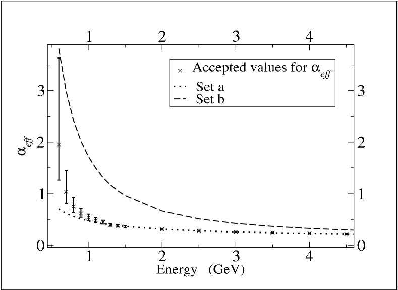
FIG. 6.: Two different fits to $\alpha_{eff}$

Eq.(87) contains the effects of the quark propagating in the instanton medium as suggested in section III. An important feature is the presence of $S^{-1}_{I}$ instead of $S^{-1}_{0}$ in the inhomogeneous term, which occurs also in Eqs. (80, 84), but not in Eq.(82). In fact, Eq.(80) is an approximation to Eq.(87) up to terms of order $\raisebox{-2.15277pt}{\mbox{$\Sigma_{I}$}}\left(S(p)-S_{I}(p)\right)$, which can be considered small, as opposed to $S^{-1}_{0}-S^{-1}_{I}$, which obviously is not small.

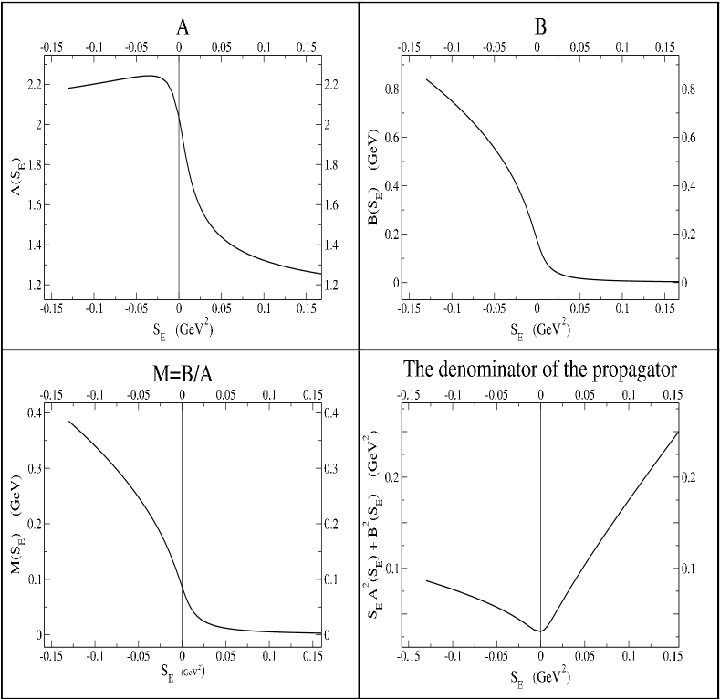
FIG. 7.: Solutions to Eq.(78) using set a. The left part of the graphs ($S_{E}<0$) represents the time-like region.

The results obtained with Eq.(78) (no instanton effects) set b, appear closer to the correct values, often overestimating them. This is most likely due to the fact that set b contains stronger infrared enhancement and overestimates the coupling the intermediate region. A comparison of both sets in terms of how they fit the accepted values of $\alpha_{eff}$ is given in Fig. 6. Inclusion of the instanton effects with set b, in most cases, do not lead to worse overestimation, as could be naively expected. With set a we have a situation where the polynomial part of our model is contributing very little in the intermediate region (which we believe to be crucial to the quantities we are computing), and the instanton effects bring in the bulk of the contribution. With set b both parts are contributing significantly, but their effects do not add. Thinking along the lines of Eq.(86), this probably means that the two types of diagrams are of different nature and not always interfere constructively. This suggests that the instanton effects are not being double-counted with this procedure, although such conjecture needs further testing.

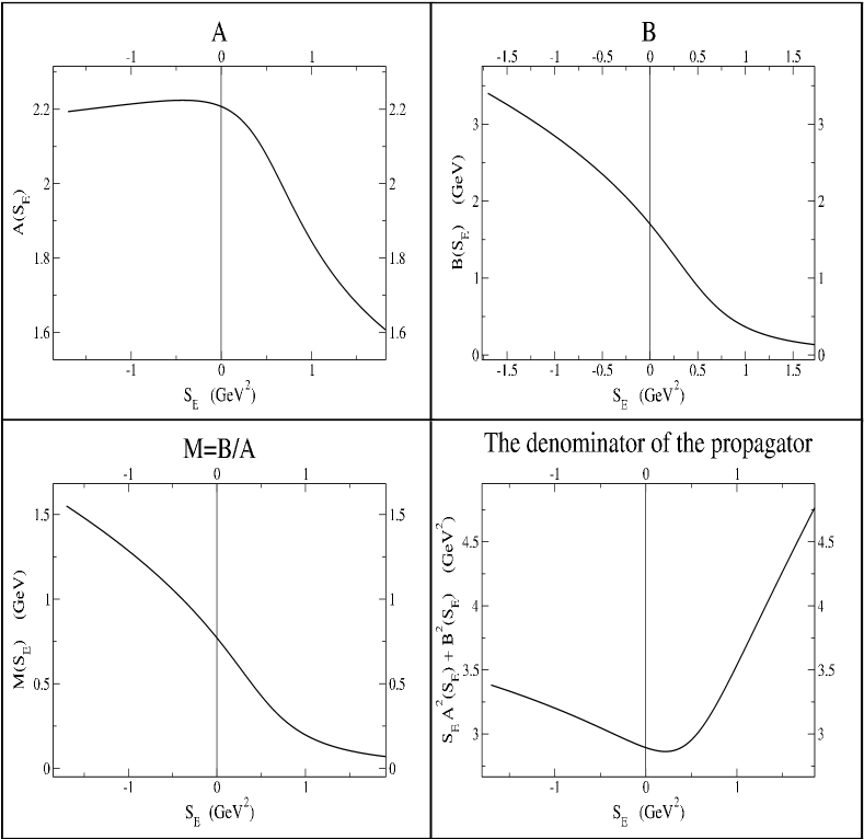
FIG. 8.: Solutions to Eq.(78) using set b. The left part of the graphs ($S_{E}<0$) represents the time-like region.

Figures 7 and 8 show graphs of the solutions obtained using set a and set b, respectively, and Eq. (78). The focus is on the low energy space-like region (right half of the graphs) and the cross-over to the time-like region (left half of the graphs). Already at small time-like energies (the graphs show energies up to about 360 MeV for set a and 1.3 GeV for set b) the behavior of the functions has changed dramatically from their behavior in the space-like region. The function $A$, for example, stops growing; and, say, the function $M$ for set a, (see Fig 7) which has barely risen from its asymptotic value of $M(p^{2})\to m_{c}=0$ at large space-like $p^{2}$ to about 90 MeV at $p^{2}=0$, is already close to 400 MeV at $p^{2}\approx(360MeV)^{2}$.

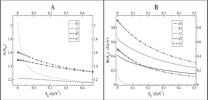
FIG. 9.: Solutions to the Schwinger-Dyson equation using set a in the space-like region. a) Result Eq.(14) from Ref[26], b) Eq.(26), c) Eq.(27), d) Eq.(28), (e) Eq.(29). In (a) $A=1$.

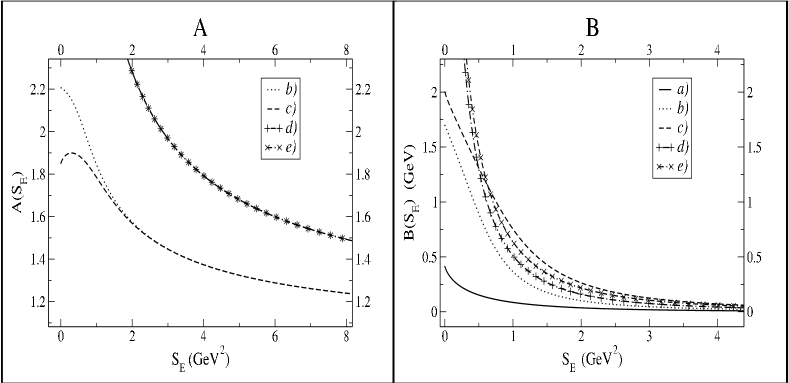
FIG. 10.: Solutions to the Schwinger-Dyson equation using set b in the space-like region. a) Result Eq.(14) from Ref[26], b) Eq.(26), c) Eq.(27), d) Eq.(28), (e) Eq.(29). In (a) $A=1$.

Of interest is also the behavior of the function $D\left(S_{E}\right)\equiv S_{E}A^{2}\left(S_{E}\right)+B^{2}\left(S_{E}\right)$, the denominator of the propagator. The vanishing of this function would indicate a pole in the quark propagator. Extrapolation of the behavior in the space-like region would suggest a pole at much smaller time-like energies than those we have plotted, particularly for set a (for set b some turning around is already noticeable at very low space-like energies). The behavior of $D$ right around its zero, if there is one, would be difficult to extract, since the functions $A\mbox{ and }B$ become singular there. In fact, $D$ seems to drop fast just to the left of the regions we have plotted. Thus, there seems to be a pole in the quark propagator on the real axis, in our polynomial model. The pole would be at $p^{2}\approx(360\mbox{ MeV})^{2}$ for set a, and $p^{2}\approx(1.3\mbox{ GeV})^{2}$ for set b. Further investigation of the solutions deeper into the time like region, is necessary before this can be ascertained. Notice that this refers to Eq.(78) only.

Figures 9 and 10 compare the solutions to Eqs.(80, 82, 84) for set a and set b, respectively. They include only the space-like region (Euclidean space), since they use the result (17) from [26], which was obtained in Euclidean space. The analytic continuation of result (17) into the time-like region exhibits a branch point at $p^{2}=0$ and thus has not been used.

VII Conclusions.

We have shown how to obtain a light-cone form of the Schwinger-Dyson equation for the quark propagator. For QCD the key question is the infra-red behavior of the gluon propagator, for which we have used two models. Knowing that the ’tHooft model[14] gives confinement, we have used polynomial models for the gluon propagator based on that model. Although the instanton liquid form[15] for the gluon propagator does not confine, and therefore does not have the correct far infra-red behavior, it provides the main mid-range QCD interaction, and allows fits to the condensates, which is essential for obtaining hadronic properties. With our approach we can obtain solutions for both the enhanced infra-red behavior of the polynomial type models or the regular infra-red behavior of the instanton model and recent lattice gauge calculations[22]. With the polynomial models we are able to work in Minkowski space and obtain solutions. With the models that include instanton effects we are able to obtain solutions that give much better agreement with the phenomenological values of the condensates.

We consider the present work is exploratory. It provides the framework for obtaining light-cone QCD propagators that can be used to obtain light-cone models of hadronic BS amplitudes for studies of hadronic properties at all momentum transfers.

Acknowledgments

This work was supported in part by the NSF grant PHY-00070888. The authors would like to thank the P25 group at Los Alamos National Laboratory for hospitality when part of this work was done, Andrew Harey and Montaga Aw for many helpful discussions. We would especially like to thank Pieter Maris for providing us with his Ph.D. thesis.

REFERENCES

- [1] P.M. Dirac, Rev. Mod. Phys. 21, 392 (1949).
- [2] C. Itzykson, and Zuber, J. B., “Quantum Field Theory” , McGraw-Hill, NY (1986).
- [3] M. Baker, J.S. Ball and F. Zachariasen, F.,Nucl. Phys. B186 531(1981).
- [4] C. Roberts and A.G. Williams, Prog. Part. Nucl. Phys. 33 447 (1994).
- [5] S. Coleman, “Aspects of symmetry”, Cambridge University Press (1988).
- [6] D. Atkinson and D.W.E. Blatt, Nucl. Phys.B151, 342 (1979).
- [7] P. Maris, “Nonperturbative analysis of the fermion propagator: complex singularities and dynamical mass generation” (PhD. dissertation,Institute for Theoretical Physics in Groningen (1993)).
- [8] Ç. Şavkli, “Quark-Antiquark Bound States within a Dyson-Schwinger Bethe-Salpeter Formalism” (PhD. dissertation, University of Pittsburgh (1997)).
- [9] S.Chang and S. Ma, Phys. Rev. 180, 1506 (1969).
- [10] G.P. Lepage and S.J. Brodsky, Phys. Rev. 22,2157 (1980).
- [11] O.C. Jacob and L.S. Kisslinger, Phys. Rev. 56, 225 (1986); Phys. Lett. 243, 323 (1990).
- [12] L.S. Kisslinger and S.W. Wang, Nucl. Phys.B399, 63 (1993).
- [13] P.C. Tandy, Prog. Part. Nucl. Phys 39, 117 (1997)
- [14] G. ’tHooft, Nucl. Phys. 75, 461 (1974).
- [15] T. Schaefer and E.V. Shuryak, Rev. Mod. Phys. 70, 323 (1998).
- [16] U. Bar-Gadda Nucl. Phys. B163, 312 (1980)
- [17] Particle Data Group, Review of Particle Physics, The European Physical Journal C15, 1 (2000).
- [18] N. Brown and M.R. Pennington, Phys. Rev. D38, 2266 (1988).
- [19] A. Hauck, R. Alkofer and l. von Smekal, L., hep-ph/9804387
- [20] F.D.R. Bonnet, P.O. Bowman, D. Leinweber and A.G. Williams, hep-lat/0002020.
- [21] J.S. Ball and T.W. Chiu, T. W., Phys. Rev. D22,2250 (1980).
- [22] C.J. Burden C.D. Roberts, Phys. Rev. D47, 5581 (1993).
- [23] D.C. Curtis and M.R. Pennington, Phys. Rev. D42, 4165 (1990).
- [24] A.A. Belavin, A.M. Polyakov, A.S. Schwartz and Yu.S. Tyupkin, Phys. Lett. B59 (1975) 85.
- [25] G.’t Hooft, Phys. Rev. D14 (1976) 3432.
- [26] P.V. Pobylitsa, Phys. Lett. 226 (1989) 387.