SAGA-HE-176-01, TMU-NT-01-04
 
 
Polarized light-antiquark distributions in a meson-cloud model

Abstract

Flavor asymmetry is investigated in polarized light-antiquark distributions by a meson-cloud model. In particular, $\rho$ meson contributions to $\Delta\bar{u}-\Delta\bar{d}$ are calculated. We point out that the $g_{2}$ part of $\rho$ contributes to the structure function $g_{1}$ of the proton in addition to the ordinary longitudinally polarized distributions in $\rho$. This kind of contribution becomes important at medium $x$ ($>0.2$) with small $Q^{2}$ ($\sim$1 GeV²). Including $N\rightarrow\rho N$ and $N\rightarrow\rho\Delta$ splitting processes, we obtain the polarized $\rho$ effects on the light-antiquark flavor asymmetry in the proton. The results show $\Delta\bar{d}$ excess over $\Delta\bar{u}$, which is very different from some theoretical predictions. Our model could be tested by experiments in the near future.

I Introduction

Light antiquark distributions are expected to be almost flavor symmetric according to perturbative quantum chromodynamics (QCD). The next-to-leading-order effects contribute to the difference between $\bar{u}$ and $\bar{d}$; however, the contribution is tiny as long as they are estimated in the perturbative QCD region. Therefore, it was rather surprising to find the antiquark flavor asymmetry $\bar{u}/\bar{d}$ in Gottfried-sum-rule violation by the New Muon Collaboration (NMC) nmc and in succeeding Drell-Yan and semi-inclusive measurements of the CERN-NA51 na51 , Fermilab-E866/NuSea e866 , and HERMES hermesud collaborations . In particular, the E866/NuSea experimental results played an important role in establishing the flavor asymmetry by clarifying the $x$ dependence of $\bar{u}/\bar{d}$. This new experimental finding was a good opportunity of investigating a mysterious nonperturbative aspect of hadron structure.

Various models have been proposed to explain the unpolarized flavor asymmetry. So far, meson-cloud type models are successful in explaining the experimental results. For the explanation of these models and other ideas, the authors suggest reading the summary papers in Ref. udsum . Since most theoretical papers are written after the NMC finding, the actual test of the proposed models should be done by predicting unobserved quantities. In this sense, the polarized light-antiquark flavor asymmetry should be an appropriate one. In fact, there are already several papers on this topic by phenomenological hadron models in Refs. models ; fs ; cs . It is particularly interesting to find that a meson-cloud model and a chiral-soliton model predict totally different contributions to $\Delta\bar{u}-\Delta\bar{d}$, although their results are similar in the unpolarized distribution $\bar{u}-\bar{d}$.

The situation of the polarized antiquark distributions is not as good as the unpolarized one in the sense that the polarized whole sea-quark distribution itself is not well determined at this stage. Most parametrizations assume flavor symmetric polarized antiquark distributions, which are then determined mainly by the $g_{1}$ measurements. As a result, there is much uncertainty in the antiquark distributions at small and large $x$ aac ; para . Although there are some semi-inclusive data semi which could be sensitive to the light antiquark flavor asymmetry, they are not accurate enough to provide strong constraint for the polarized antiquark flavor asymmetry para ; semi . However, the Relativistic Heavy Ion Collider (RHIC) rhic and the Common Muon and Proton Apparatus for Structure and Spectroscopy (COMPASS) compass experiments should clarify the details of the polarized antiquark distributions in a few years. It is the right time to investigate the antiquark flavor asymmetry $\Delta\bar{u}/\Delta\bar{d}$ by possible theoretical models and to summarize various predictions.

In this paper, we intend to shed light on the virtual meson model which has been successful in the unpolarized studies meson . The purpose of this paper is to extend the studies of the virtual $\rho$-meson contributions by Fries and Schäfer in Ref. fs . In particular, we point out that the $g_{2}$ part of the polarized $\rho$ contributes to the polarized flavor asymmetry in addition to the ordinary longitudinal part, which was calculated in Ref. fs . Because we show new $g_{2}$ terms in this paper and because the situation is still confusing in the sense that another $\rho$-meson paper cs claims major differences from Ref. fs in supposedly the same $\rho$ contributions, the detailed formalism is shown in the following sections. The meson model was extended recently to a different direction in Ref. cs by including $\pi-\rho$ interference terms; however, this paper is intended to investigate a different kinematical aspect within the meson model.

The paper consists of the following. The formalism of $\rho$ contributions to $\Delta\bar{u}-\Delta\bar{d}$ is presented in Sec. II. Meson momentum distributions are obtained in Sec. III, and numerical results of $\Delta\bar{u}-\Delta\bar{d}$ are shown in Sec. IV. Our studies are summarized in Sec. V.

II Vector-meson contributions

The cross section of polarized electron-nucleon scattering is generally written in terms of lepton and hadron tensors:

$$\frac{d\sigma}{dE_{e}^{\prime}d\Omega_{e}^{\prime}}=\frac{|\vec{p}_{e}^{\,\prime}|}{|\vec{p}_{e}|}\,\frac{\alpha^{2}}{(q^{2})^{2}}\,L^{\mu\nu}(p_{e},s_{e},q)\,W_{\mu\nu}(p_{N},s_{N},q),$$ (1)

where $\alpha$ is the fine structure constant, $E_{e}^{\prime}$ and $\Omega_{e}^{\prime}$ are the scattered electron energy and solid angle, and $p_{e}$, $p_{e}^{\prime}$, $p_{N}$, and $q$ are initial electron, final electron, nucleon, and virtual photon momenta, respectively. The electron and nucleon spins are expressed by $s_{e}$ and $s_{N}$ with the normalization $s_{e}^{2}=s_{N}^{2}=-1$. Throughout this paper, the convention $-g_{00}=g_{11}=g_{22}=g_{33}=+1$ is used so as to have, for example, $p_{N}^{2}=(p_{N}^{0})^{2}-\vec{p}_{N}^{\,\,2}=m_{N}^{2}$. Furthermore, the Dirac spinor is normalized as $u^{\dagger}u=E_{e}/m_{e}$ or $E_{N}/m_{N}$, where $E_{e}$ and $E_{N}$ are electron and nucleon energies, and $m_{e}$ and $m_{N}$ are their masses. The polarized lepton and hadron tensors are given by

$$L^{\mu\nu}(p_{e},s_{e},q)=2\,\big{[}\,p_{e}^{\mu}{p_{e}^{\prime}}^{\nu}+p_{e}^{\nu}{p_{e}^{\prime}}^{\mu}-(p_{e}\cdot p_{e}^{\prime}-m_{e}^{2})\,g^{\mu\nu}$$

$$\ \ \ \ \ \ \ \ \ \ \ \ \ \ \ \ \ \ \ \ \ \ \ \ \ -i\,\varepsilon^{\mu\nu\rho\sigma}m_{e}q_{\rho}s_{e\,\sigma}\,\big{]},$$ (2)

$$W_{\mu\nu}(p_{N},s_{N},q)=\frac{1}{2\pi}\sum_{X}\,(2\pi)^{4}\,\delta^{4}(p_{N}+q-p_{{}_{X}})$$

$$\ \ \ \ \ \times<p_{N},s_{N}|J_{\mu}(0)|\,X>\,<X|J_{\nu}(0)|\,p_{N},s_{N}>,$$ (3)

where the factor $\varepsilon^{\mu\nu\rho\sigma}$ is the antisymmetric tensor with the convention $\epsilon_{0123}=+1$.

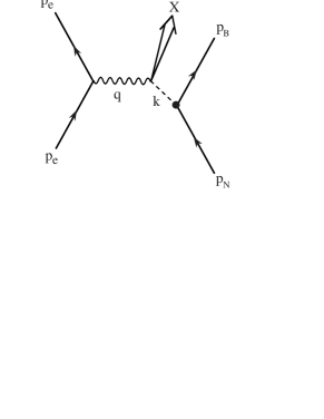
Figure 1: Virtual vector-meson contribution.

Next, we consider the process in Fig. 1, where the nucleon splits into a virtual vector meson and a baryon, then the virtual photon interacts with the polarized meson. Because scalar mesons do not contribute directly to the polarized structure functions due to spinless nature, the lightest vector meson, namely $\rho$, is taken into account in this paper. In future, we may extend the present studies by including heavier vector mesons. As the final state baryon, the nucleon and $\Delta$ are considered. Expressing the $VNB$ vertex multiplied by the meson propagator as $J_{VNB}(k,s_{V},p_{N},s_{N},p_{B},s_{B})$ and calculating the cross section due to the process in Fig. 1, we obtain

$$\frac{d\sigma}{dE_{e}^{\prime}d\Omega_{e}^{\prime}}=\frac{|\vec{p}_{e}^{\,\prime}|}{|\vec{p}_{e}|}\,\frac{\alpha^{2}}{(q^{2})^{2}}\,L^{\mu\nu}(p_{e},s_{e},q)$$

$$\times\,\int\frac{d^{3}p_{B}}{(2\pi)^{3}}\,\frac{m_{B}}{2\pi E_{B}}\sum_{X,\lambda_{V},\lambda_{B}}|J_{VNB}|^{2}<k,s_{V}|J_{\mu}(0)|\,X>$$

$$\times\,<X|J_{\nu}(0)|\,k,s_{V}>(2\pi)^{4}\,\delta^{4}(k+q-p_{{}_{X}}).$$ (4)

Here, $k$ and $s_{V}$ indicate the meson momentum and spin. This equation has the same form as Eq. (1). Therefore, the last part is identified with a vector-meson contribution to the nucleon tensor:

$$W_{\mu\nu}(p_{N},s_{N}, q)=\int\frac{d^{3}p_{B}}{(2\pi)^{3}}\,\frac{2m_{V}m_{B}}{E_{B}}$$

$$\times\sum_{\lambda_{V},\lambda_{B}}|J_{VNB}|^{2}\,W_{\mu\nu}^{(V)}(k,s_{V},q),$$ (5)

where $m_{V}$ is the meson mass, and the meson tensor is defined by

$$W_{\mu\nu}^{(V)} (k,s_{V},q)=\frac{1}{4\pi m_{V}}\sum_{X}(2\pi)^{4}\,\delta^{4}(k+q-p_{{}_{X}})$$

$$\times<k,s_{V}|J_{\mu}(0)|\,X>\,<X|J_{\nu}(0)|\,k,s_{V}>.$$ (6)

In this way, the vector-meson contribution to the nucleon tensor is expressed in terms of the $VNB$ vertex and the meson tensor. Because we are interested in meson effects on the polarized parton distributions in the nucleon, we try to project the $g_{1}$ part out from the nucleon tensor. The definition of the $g_{1}$ and $g_{2}$ structure functions is given in the asymmetric part of the nucleon tensor:

$$W^{A}_{\mu\nu}(p_{N}, s_{N},q)=i\,\varepsilon_{\mu\nu\rho\sigma}\,q^{\,\rho}\bigg{[}\,s_{N}^{\,\sigma}\,\frac{g_{1}}{p_{N}\cdot q}$$

$$+(p_{N}\cdot q\,s_{N}^{\,\sigma}-s_{N}\cdot q\,p_{N}^{\,\sigma})\,\frac{g_{2}}{(p_{N}\cdot q)^{2}}\,\bigg{]}.$$ (7)

In order to discuss each structure function separately, a projection operator

$$P^{\mu\nu}=-\frac{m_{N}^{2}}{2\,p_{N}\cdot q}\,i\,\varepsilon^{\mu\nu\alpha\beta}\,q_{\alpha}\,s_{N\,\beta},$$ (8)

is then applied to give

$$P^{\mu\nu}\,W^{A}_{\mu\nu}(p_{N},s_{N},q)=\frac{m_{N}^{2}}{(p_{N}\cdot q)^{2}}\left[q^{2}+(s_{N}\cdot q)^{2}\right]\,g_{1}-\gamma^{2}\,g_{2}.$$ (9)

Here, $\gamma$ is defined by

$$\gamma^{2}=\frac{4\,x^{2}\,m_{N}^{2}}{Q^{2}},$$ (10)

with $Q^{2}=-q^{2}$. In the same way, $g_{1}$ and $g_{2}$ structure functions of the vector meson are defined in the asymmetric part of the tensor. Operating the projection also on the meson tensor, we obtain

$$P^{\mu\nu}W^{(V)A}_{\mu\nu}(k,s_{V},q)=\frac{m_{N}}{m_{V}}\,[\,A_{1}\,g_{1}^{V}(k,q)+A_{2}\,g_{2}^{V}(k,q)\,],$$ (11)

where $A_{1}$ and $A_{2}$ are given by

$$A_{1} =\frac{m_{N}\,m_{V}}{p_{N}\cdot q\,k\cdot q}\,(s_{N}\cdot q\,s_{V}\cdot q-q^{2}s_{N}\cdot s_{V}),$$ (12)

$$A_{2} =\frac{m_{N}\,m_{V}\,q^{2}}{p_{N}\cdot q\,(k\cdot q)^{2}}\,(s_{N}\cdot k\,s_{V}\cdot q-k\cdot q\,s_{N}\cdot s_{V}).$$ (13)

From Eqs. (5), (9), and (11), the meson contribution to the nucleon structure functions becomes

$$\frac{m_{N}^{2}}{(p_{N}\cdot q)^{2}}\,[\,q^{2}+(s_{N}\cdot q)^{2}\,]\,g_{1}(p_{N},q)-\gamma^{2}\,g_{2}(p_{N},q)$$

$$\ \ \ \ =\int\frac{d^{3}p_{B}}{(2\pi)^{3}}\,\frac{2m_{N}m_{B}}{E_{B}}\sum_{\lambda_{V},\lambda_{B}}|J_{VNB}|^{2}$$

$$\ \ \ \ \ \ \ \ \ \ \ \ \times\,[\,A_{1}\,g_{1}^{V}(k,q)+A_{2}\,g_{2}^{V}(k,q)\,].$$ (14)

Then, the above integration variables ($p_{B}^{x}$, $p_{B}^{y}$, $p_{B}^{z}$) are changed for the meson momentum fraction $y$, the transverse momentum $k_{\perp}$ of the meson, and the angle $\phi$ between $\vec{k}_{\perp}$ and the transverse spin vector of the nucleon ($\vec{s}_{N}^{\,T}$):

$$y=\frac{k\cdot q}{p_{N}\cdot q}\ ,\ \ \ \ \ \vec{k}\cdot\vec{s}_{N}^{\,T}=k_{\perp}\tau_{N}\cos\phi,$$ (15)

with $\tau_{N}=|\vec{s}_{N}^{\,T}|$. Then, the meson contribution is expressed as

$$\frac{m_{N}^{2}}{(p_{N}\cdot q)^{2}}\,[\,q^{2}+(s_{N}\cdot q)^{2}\,]\,g_{1}(x,Q^{2})-\gamma^{2}\,g_{2}(x,Q^{2})$$

$$=\int_{x}^{1}\frac{dy}{y}\,[\,B_{1}(y)\,g_{1}^{V}(x/y,Q^{2})+B_{2}(y)\,g_{2}^{V}(x/y,Q^{2})\,].$$ (16)

The upper limit of the $y$-integration range is taken as 1 by considering the vector-meson mass smaller than the nucleon mass. However, one should be careful in extending the present studies to other mesons with larger masses. The meson momentum distributions are expressed as

$$B_{1,2}(y)= \int_{0}^{(\vec{k}_{\perp}^{\,2})_{max}}d\vec{k}_{\perp}^{\,2}\int_{0}^{2\pi}d\phi\frac{|\vec{p}_{N}|\,m_{N}\,m_{B}}{(2\pi)^{3}E_{B}}\,\frac{\partial y^{\prime}}{\partial y}\,y$$

$$\times\sum_{\lambda_{V},\lambda_{B}}|J_{VNB}|^{2}\,A_{1,2}\ ,$$ (17)

where $y^{\prime}$ is the longitudinal momentum fraction defined in the meson momentum

$$\vec{k}=\vec{k}_{\perp}+y^{\prime}\vec{p}_{N}.$$ (18)

In the infinite momentum frame $|\vec{p}_{N}|\rightarrow\infty$, $y$ and $y^{\prime}$ are related by

$$y^{\prime}=\frac{y}{1+\sqrt{1+\gamma^{2}}}\,\bigg{[}\,1+\sqrt{1+\frac{\gamma^{2}}{y^{2}m_{N}^{2}}(\vec{k}_{\perp}^{2}+m_{V}^{2})}\,\bigg{]}.$$ (19)

Because time-ordered perturbation theory is used for the reaction in Fig. 1 as explained in Sec. III, the vector meson is taken as an on-shell particle: $k^{2}=m_{V}^{2}$ in the above derivation. The partial derivative $\partial y^{\prime}/\partial y$ can be calculated from this expression. In the infinite momentum frame, the momentum fraction $y^{\prime}$ has to satisfy the kinematical condition $0\leq y^{\prime}\leq 1$, namely the meson $V$ and the baryon $B$ should move in the forward direction. The maximum transverse momentum is given by

$$(\vec{k}_{\perp}^{\,2})_{max}=\frac{m_{N}^{2}}{\gamma^{2}}\,(\sqrt{1+\gamma^{2}}+1)\,(\sqrt{1+\gamma^{2}}+1-2y)-m_{V}^{2}.$$ (20)

Practically, it does not matter to take the upper bound $(\vec{k}_{\perp}^{\,2})_{max}\rightarrow\infty$ in Eq. (17) at small-$x$ where the antiquark distributions play a major role, because $(\vec{k}_{\perp}^{\,2})_{max}$ $(\sim Q^{2}(1-y)/x^{2}\gg m_{N}^{2})$ is beyond the vertex momentum cutoff region discussed in Sec. III. The contribution to the integral between $(\vec{k}_{\perp}^{\,2})_{max}$ and $\vec{k}_{\perp}^{\,2}=\infty$ is extremely small in general. Furthermore, the upper bound becomes $(\vec{k}_{\perp}^{\,2})_{max}\rightarrow\infty$ in the limit $Q^{2}\rightarrow\infty$, and it is consistent with the previous publications fs ; cs . In this way, the meson contribution is expressed in terms of the meson structure functions convoluted with the meson momentum distributions in the nucleon.

Using the integration variables $y$, $\vec{k}_{\perp}^{2}$, and $\phi$, we express the coefficients $A_{1}$ and $A_{2}$ as

$$A_{1}= \lambda_{N}\lambda_{V}\bigg{[}1+\frac{\vec{k}_{\perp}^{2}}{yy^{\prime}\,m_{N}^{2}}(\sqrt{1+\gamma^{2}}-1)\bigg{]}$$

$$\ \ \ \ -\gamma^{2}\tau_{N}\lambda_{V}\cos\phi\,\frac{k_{\perp}}{y\,m_{N}},$$

$$A_{2}= \frac{\gamma^{2}m_{V}^{2}}{y^{2}m_{N}^{2}}\bigg{[}\,-\lambda_{N}\lambda_{V}+\tau_{N}\lambda_{V}\!\cos\phi\,\frac{k_{\perp}}{y^{\prime}\,m_{N}}\,(\sqrt{1+\gamma^{2}}-1)\,\bigg{]},$$ (21)

in the limit $|\vec{p}_{N}|\rightarrow\infty$. Detailed calculations indicate that $\phi$ dependence can be extracted out from another part of the integrand in Eq.(17) as

$$\frac{|\vec{p}_{N}|\,m_{N}\,m_{B}}{(2\pi)^{3}E_{B}}\,\frac{\partial y^{\prime}}{\partial y}\,y\sum_{\lambda_{B}}|J_{VNB}|^{2}\equiv C_{L}^{\lambda_{V}}+\tau_{N}\cos\phi\,C_{T}^{\lambda_{V}}\ .$$ (22)

Then, after the $\phi$ integration, Eq. (17) becomes

$$B_{1}(y) =\sum_{\lambda_{V}}\lambda_{V}\,[\lambda_{N}\,f_{1L}^{\lambda_{V}}(y)-\tau_{N}^{2}\,f_{1T}^{\lambda_{V}}(y)],$$ (23)

$$B_{2}(y) =\sum_{\lambda_{V}}\lambda_{V}\,[-\lambda_{N}\,f_{2L}^{\lambda_{V}}(y)+\tau_{N}^{2}\,f_{2T}^{\lambda_{V}}(y)],$$ (24)

where $\lambda_{V}$ dependence is explicitly denoted in meson momentum distributions, which are defined by

$$f_{1L}^{\lambda_{V}}(y) =\int_{0}^{(\vec{k}_{\perp}^{\,2})_{max}}\!\!\!d\vec{k}_{\perp}^{\,2}2\pi\,C_{L}^{\lambda_{V}}\,\bigg{[}1+\frac{\vec{k}_{\perp}^{2}}{yy^{\prime}m_{N}^{2}}(\sqrt{1+\gamma^{2}}-1)\bigg{]}\,,$$ (25)

$$f_{1T}^{\lambda_{V}}(y) =\int_{0}^{(\vec{k}_{\perp}^{\,2})_{max}}\!\!\!d\vec{k}_{\perp}^{\,2}\gamma^{2}\,\pi\,C_{T}^{\lambda_{V}}\,\frac{k_{\perp}}{ym_{N}}\,,$$ (26)

$$f_{2L}^{\lambda_{V}}(y) =\int_{0}^{(\vec{k}_{\perp}^{\,2})_{max}}\!\!\!d\vec{k}_{\perp}^{\,2}\gamma^{2}\,2\pi\,C_{L}^{\lambda_{V}}\,\frac{m_{V}^{2}}{y^{2}m_{N}^{2}}\,,$$ (27)

$$f_{2T}^{\lambda_{V}}(y) =\int_{0}^{(\vec{k}_{\perp}^{\,2})_{max}}\!\!\!d\vec{k}_{\perp}^{\,2}\gamma^{2}\,\pi\,C_{T}^{\lambda_{V}}\,\frac{k_{\perp}m_{V}^{2}}{y^{\prime}y^{2}m_{N}^{3}}(\sqrt{1+\gamma^{2}}-1)\,.$$ (28)

Because the functions $f_{1T}^{\lambda_{V}}$, $f_{2L}^{\lambda_{V}}$, and $f_{2T}^{\lambda_{V}}$ are proportional to $\gamma^{2}$, they vanish in the limit $Q^{2}\rightarrow\infty$. As it is obvious from Eq. (16), it is necessary to consider both longitudinal and transverse polarizations for the nucleon in order to extract the $g_{1}$ part. In addition, the $g_{2}$ structure function of the meson contributes. The function $f_{1L}^{\lambda_{V}}(y)$ is the ordinary meson momentum distribution with the momentum fraction $y$ in the longitudinally polarized nucleon. The function $f_{1T}^{\lambda_{V}}(y)$ is the distribution in the transversely polarized nucleon. On the other hand, $f_{2L}^{\lambda_{V}}(y)$ and $f_{2T}^{\lambda_{V}}(y)$ are the distributions associated with $g_{2}$ of the vector meson. Expressing Eq. (16) in terms of the nucleon and meson helicities, $\lambda_{N}$ and $\lambda_{V}$, we obtain

$$(\lambda_{N}^{2}-\tau_{N}^{2}\,\gamma^{2})\,g_{1}(x,Q^{2})-\gamma^{2}\,g_{2}(x,Q^{2})$$

$$=\sum_{\lambda_{V}}\lambda_{V}\int_{x}^{1}\frac{dy}{y}\,\big{[}\,\big{\{}\lambda_{N}\,f_{1L}(y)-\tau_{N}^{2}\,f_{1T}(y)\big{\}}\,g_{1}^{V}(x/y,Q^{2})$$

$$\ \ \ \ +\big{\{}-\lambda_{N}\,f_{2L}(y)+\tau_{N}^{2}\,f_{2T}(y)\big{\}}\,g_{2}^{V}(x/y,Q^{2})\,\big{]}.$$ (29)

Combining the longitudinal polarization $\lambda_{N}=1$ ($\tau_{N}=0$) with the transverse polarization $\tau_{N}=1$ ($\lambda_{N}=0$), we can extract the $g_{1}$ part as

$$g_{1}(x,Q^{2})=\frac{1}{1+\gamma^{2}}\int_{x}^{1}\frac{dy}{y}$$

$$\ \ \times\,\big{[}\,\big{\{}\Delta f_{1L}(y)+\Delta f_{1T}(y)\big{\}}\,g_{1}^{V}(x/y,Q^{2})$$

$$\ \ \ \ \ -\big{\{}\Delta f_{2L}(y)+\Delta f_{2T}(y)\big{\}}\,g_{2}^{V}(x/y,Q^{2})\,\big{]},$$ (30)

where the functions $\Delta f_{i}^{VN}(y)$ with $i$=$1L$, $2L$, $1T$, and $2T$ are defined by

$$\Delta f_{i}(y)=f_{i}^{\lambda_{V}=+1}(y)-f_{i}^{\lambda_{V}=-1}(y).$$ (31)

The $g_{2}$ part is obtained in the same way as

$$g_{2}(x,Q^{2})=\frac{1}{1+\gamma^{2}}\int_{x}^{1}\frac{dy}{y}$$

$$\ \ \times\,\big{[}\,\big{\{}-\Delta f_{1L}(y)+\Delta f_{1T}(y)/\gamma^{2}\big{\}}\,g_{1}^{V}(x/y,Q^{2})$$

$$\ +\big{\{}\Delta f_{2L}(y)-\Delta f_{2T}(y)/\gamma^{2}\big{\}}\,g_{2}^{V}(x/y,Q^{2})\,\big{]}.$$ (32)

In the limit $Q^{2}\rightarrow\infty$, namely $\gamma^{2}\rightarrow 0$, only the momentum distribution $\Delta f_{1L}(y)$ remains finite, and Eq. (30) agrees with the expression in Ref. fs .

In Eq. (30), there are additional terms associated with $g_{2}$ of the meson. For discussing these $g_{2}$ type contributions to $\Delta\bar{u}-\Delta\bar{d}$, $g_{2}^{V}$ is approximated by the Wandzura-Wilczek (WW) relation ww by neglecting higher-twist terms:

$$g_{2}^{V(WW)}(x,Q^{2})=-g_{1}^{V}(x,Q^{2})+\int_{x}^{1}\frac{dy}{y}g_{1}^{V}(y,Q^{2}).$$ (33)

Then, providing the leading-order expression for $g_{1}^{V}$, we have

$$g_{2}^{V(WW)}(x,Q^{2})=\frac{1}{2}\sum_{i}\,e_{i}^{2}\,[\, \Delta q_{i}^{V(WW)}(x,Q^{2})$$

$$+ \Delta\bar{q}_{i}^{V(WW)}(x,Q^{2})\,].$$ (34)

The above WW distributions are defined by

$$\Delta\bar{q}_{i}^{V(WW)}(x,Q^{2})=-\Delta\bar{q}_{i}^{V}(x,Q^{2})+\int_{x}^{1}\frac{dy}{y}\,\Delta\bar{q}_{i}^{V}(y,Q^{2}),$$ (35)

and the same equation for $\Delta q_{i}^{V(WW)}(x,Q^{2})$. From these equations, we obtain a vector meson contribution to the polarized antiquark distribution $\Delta\bar{q}_{i}$ in the proton as

$$\Delta\bar{q}_{i}^{VNB}(x,Q^{2})=\frac{1}{1+\gamma^{2}}\int_{x}^{1}\frac{dy}{y}$$

$$\ \times\,\big{[}\,\big{\{}\Delta f_{1L}(y)+\Delta f_{1T}(y)\big{\}}\,\Delta\bar{q}_{i}^{V}(x/y,Q^{2})$$

$$\ \ \ \ -\big{\{}\Delta f_{2L}(y)+\Delta f_{2T}(y)\big{\}}\,\Delta\bar{q}_{i}^{V(WW)}(x/y,Q^{2})\,\big{]}.$$ (36)

If this kind of vector-meson contribution is the only source for the polarized flavor asymmetry, the $\Delta\bar{u}-\Delta\bar{d}$ distribution is then calculated by taking the difference $\Delta\bar{q}_{i=u}^{VNB}-\Delta\bar{q}_{i=d}^{VNB}$ in the above equation.

III Meson momentum distributions

In order to estimate the meson contributions numerically, it is necessary to calculate the momentum distributions $\Delta f_{i}^{VN}(y)$ of the meson. We calculate them by considering the vector-meson creation processes $N\rightarrow VN^{\prime}$ and $N\rightarrow V\Delta$ through the interactions

$$V_{VNN} =\widetilde{\phi}_{V}^{*}\cdot\widetilde{T}\,F_{VNN}(k)\,\,\overline{u}(p_{N}^{\prime},s_{N}^{\prime})\,\varepsilon^{\mu\,*}$$

$$\ \ \ \ \times\bigg{[}\,g_{V}\gamma_{\mu}-\frac{f_{V}}{2m_{N}}\,i\,\sigma_{\mu\nu}\widehat{K}^{\nu}\,\bigg{]}\,\,u(p_{N},s_{N}),$$ (1)

$$V_{VN\Delta} =\widetilde{\phi}_{V}^{*}\cdot\widetilde{T}\,F_{VN\Delta}(k)\,\,\overline{U}_{\nu}(p_{\Delta},s_{\Delta})\,\frac{f_{VN\Delta}}{m_{V}}\,\gamma_{5}\,\gamma_{\mu}$$

$$\times\,\big{[}\,\widehat{K}^{\mu}\,\varepsilon^{\nu\,*}-\widehat{K}^{\nu}\,\varepsilon^{\mu\,*}\,\big{]}\,u(p_{N},s_{N}),$$ (2)

where $u(p_{N},s_{N})$ is the Dirac spinor, $U^{\mu}(p_{\Delta},s_{\Delta})$ is the Rarita-Schwinger spinor, and $\varepsilon^{\mu}$ is the polarization vector of the vector meson. The $VNN$ and $VN\Delta$ coupling constants are denoted as $g_{V}$, $f_{V}$, and $f_{VN\Delta}$, and form factors are denoted as $F_{VNN}(k)$ and $F_{VN\Delta}(k)$. Isospin dependence is taken into account by the factor $\widetilde{\phi}_{V}^{*}\cdot\widetilde{T}$, and it is defined in terms of a reduced matrix element and a Clebsch-Gordan coefficient skflux ; edmonds

$$<\!B\,|\,\widetilde{\phi}_{V}^{*}\cdot\widetilde{T}\,|\,N\!> =(-1)^{M_{V}}\frac{<T_{B}\parallel\widehat{T}\parallel T_{N}\!>}{\sqrt{2T_{B}+1}}$$

$$\times<T_{N}M_{N}:1-M_{V}|T_{B}M_{B}\!>$$ (3)

with $<1/2\parallel\widehat{T}\parallel\!1/2>=\sqrt{6}$ and $<3/2\parallel\widehat{T}\parallel\!1/2>=2$. Here, $T_{N}$ and $T_{B}$ denote isospins of the nucleon and the baryon, respectively, and $M_{N}$ and $M_{B}$ are their third components.

From these vertices, the meson momentum distribution $f_{M}(y)$ can be calculated together with the baryon distribution $f_{B}(y)$. They are supposed to satisfy the relation $f_{M}(y)=f_{B}(1-y)$ because of charge and momentum conservations. However, it is known that the covariant calculation could violate this relation because a derivative coupling introduces off-shell dependence. A possible solution julich ; mt is to use the time-ordered perturbation theory (TOPT), instead of the covariant formalism. Although the four-momentum conservation is satisfied at the $VNB$ vertex in the covariant formalism, the energy is not conserved in the TOPT topt . If there is no off-shell dependence at a vertex, the TOPT agrees certainly with the ordinary covariant theory by collecting all the time-ordered diagrams. However, the off-shell dependence due to the derivative coupling complicates the problem. It leads to a freedom in defining the vertex momentum $\widehat{K}$ in Eqs. (1) and (2). The following two possibilities are considered in Refs. fs ; julich :

(A) $$\widehat{K}=k=(E_{V},\vec{k}),$$

(B) $$\widehat{K}={\overline{k}}=p_{N}-p_{B}=(E_{N}-E_{B},\vec{k}),$$ (4)

where $E_{V}=\sqrt{m_{V}^{2}+\vec{k}^{\,2}}$. There is another off-shell dependence from the vertex form factors, and it is discussed in Sec. IV.

From the $VNN$ interaction vertex in Eq. (1), we obtain

$$\sum_{\lambda_{N}^{\prime}}|V_{VNN}|^{2}=|\widetilde{\phi}_{V}^{*}\cdot\widetilde{T}|^{2}\,F_{VNN}^{\,2}(k)\,\frac{1}{4\,m_{N}^{2}}\,\bigg{[}\,g_{V}^{2}\,\big{\{}-{\overline{k}}^{2}$$

$$\ \ \ +2\,(p_{N}\cdot\varepsilon\,p_{N}^{\prime}\cdot\varepsilon^{*}+p_{N}\cdot\varepsilon^{*}p_{N}^{\prime}\cdot\varepsilon)+2m_{N}m_{V}s_{N}\cdot\overline{s}_{V}\big{\}}$$

$$+g_{V}\,f_{V}\,\big{\{}-2{\overline{k}}\cdot\widehat{K}+2m_{N}m_{V}s_{N}\cdot\hat{s}_{V}$$

$$\ \ \ \ \ \ \ \ \ \ \ \ \ \ -2p_{N}^{\prime}\cdot\widehat{K}\,s_{N}\cdot s^{\prime}-\widehat{K}\cdot\varepsilon\,{\overline{k}}\cdot\varepsilon^{*}-\widehat{K}\cdot\varepsilon^{*}{\overline{k}}\cdot\varepsilon\,\}$$

$$+\frac{f_{V}^{2}}{4m_{N}^{2}}\,\big{\{}\,(\widehat{K}^{2}+\widehat{K}\cdot\varepsilon\,\widehat{K}\cdot\varepsilon^{*})({\overline{k}}^{2}-4m_{N}^{2})+4p_{N}\cdot\widehat{K}p_{N}^{\prime}\cdot\widehat{K}$$

$$\ \ \ -2\widehat{K}^{2}(p_{N}\cdot\varepsilon\,p_{N}^{\prime}\cdot\varepsilon^{*}+p_{N}\cdot\varepsilon^{*}p_{N}^{\prime}\cdot\varepsilon)+4m_{N}^{2}\widehat{K}^{2}s_{N}\cdot s^{\prime}$$

$$\ \ \ -4m_{N}m_{V}p_{N}^{\prime}\cdot\widehat{K}s_{N}\cdot\hat{s}_{V}-2m_{N}m_{V}\widehat{K}^{2}s_{N}\cdot\overline{s}_{V}$$

$$\ \ \ +2(p_{N}\cdot\widehat{K}+p_{N}^{\prime}\cdot\widehat{K})(p_{N}\cdot\varepsilon\,\widehat{K}\cdot\varepsilon^{*}+p_{N}\cdot\varepsilon^{*}\widehat{K}\cdot\varepsilon)$$

$$\ \ \ -2p_{N}\cdot\widehat{K}(\widehat{K}\cdot\varepsilon\,{\overline{k}}\cdot\varepsilon^{*}+\widehat{K}\cdot\varepsilon^{*}{\overline{k}}\cdot\varepsilon)\,\big{\}}\,\bigg{]}\ ,$$ (5)

where ${s^{\prime}}^{\mu}$, $\hat{s}_{V}^{\mu}$, $\overline{s}_{V}^{\mu}$ are defined by

$${s^{\prime}}^{\,\mu} =-\frac{i}{m_{N}}\,\varepsilon^{\mu\nu\alpha\beta}\,\varepsilon_{\nu}^{*}\,\varepsilon_{\alpha}\,p_{N\beta},$$ (6)

$$\hat{s}_{V}^{\,\mu} =-\frac{i}{m_{V}}\,\varepsilon^{\mu\nu\alpha\beta}\,\varepsilon_{\nu}^{*}\,\varepsilon_{\alpha}\,\widehat{K}_{\beta},$$ (7)

$$\overline{s}_{V}^{\,\mu} =-\frac{i}{m_{V}}\,\varepsilon^{\mu\nu\alpha\beta}\,\varepsilon_{\nu}^{*}\,\varepsilon_{\alpha}\,\overline{k}_{\beta}.$$ (8)

The meson polarization vector is given by

$$\varepsilon^{\mu}=\bigg{(}\frac{\vec{k}\cdot\vec{\varepsilon}_{\lambda_{V}}}{m_{V}},\vec{\varepsilon}_{\lambda_{V}}+\frac{\vec{k}\cdot\vec{\varepsilon}_{\lambda_{V}}}{m_{V}(E_{V}+m_{V})}\vec{k}\bigg{)},$$ (9)

where $\lambda_{V}$ is the meson helicity. The spherical unit vector $\vec{\varepsilon}_{\lambda_{V}}$ is defined in the frame with the $\hat{z}^{\prime}$ axis parallel to $\vec{k}$:

$$\vec{\varepsilon}_{\pm 1}=\mp\frac{1}{\sqrt{2}}(\hat{x}^{\prime}\pm i\hat{y}^{\prime}),\ \ \ \vec{\varepsilon}_{0}=\hat{z}^{\prime}.$$ (10)

In the same way, the $VN\Delta$ term is calculated from Eq. (2) as

$$\sum_{\lambda_{\Delta}}|V_{VN\Delta}|^{2}=-|\widetilde{\phi}_{V}^{*}\cdot\widetilde{T}|^{2}\,F_{VN\Delta}^{\,2}(k)\,\frac{f_{VN\Delta}^{2}}{6\,m_{N}m_{\Delta}^{3}m_{V}^{2}}$$

$$\times\bigg{[}\,-2m_{\Delta}^{2}p_{N}\cdot\widehat{K}p_{\Delta}\cdot\widehat{K}+2m_{N}m_{\Delta}^{3}(\widehat{K}^{2}+\widehat{K}\cdot\varepsilon\widehat{K}\cdot\varepsilon^{*})$$

$$\ \ +2p_{N}\cdot p_{\Delta}\big{\{}m_{\Delta}^{2}\widehat{K}^{2}+m_{\Delta}^{2}\widehat{K}\cdot\varepsilon\widehat{K}\cdot\varepsilon^{*}+\widehat{K}^{2}p_{\Delta}\cdot\varepsilon\,p_{\Delta}\cdot\varepsilon^{*}$$

$$\ \ \ \ \ \ \ \ -p_{\Delta}\cdot\widehat{K}(p_{\Delta}\cdot\varepsilon\widehat{K}\cdot\varepsilon^{*}+p_{\Delta}\cdot\varepsilon^{*}\widehat{K}\cdot\varepsilon)-(p_{\Delta}\cdot\widehat{K})^{2}\big{\}}$$

$$\ \ +m_{\Delta}^{2}\big{\{}-p_{N}\cdot\widehat{K}(p_{\Delta}\cdot\varepsilon\widehat{K}\cdot\varepsilon^{*}+p_{\Delta}\cdot\varepsilon^{*}\widehat{K}\cdot\varepsilon)$$

$$\ \ \ \ \ \ \ \ \ \ \ \ \ -p_{\Delta}\cdot\widehat{K}(p_{N}\cdot\varepsilon\widehat{K}\cdot\varepsilon^{*}+p_{N}\cdot\varepsilon^{*}\widehat{K}\cdot\varepsilon)$$

$$\ \ \ \ \ \ \ \ \ \ \ \ \ +\widehat{K}^{2}(p_{N}\cdot\varepsilon p_{\Delta}\cdot\varepsilon^{*}+p_{N}\cdot\varepsilon^{*}p_{\Delta}\cdot\varepsilon)\,\big{\}}$$

$$\ \ +m_{N}s_{N}\cdot s^{\prime}\big{\{}2m_{N}(p_{\Delta}\cdot\widehat{K})^{2}+m_{\Delta}^{2}(m_{N}+m_{\Delta})\widehat{K}^{2}\big{\}}$$

$$\ \ -m_{N}m_{V}s_{N}\cdot\overline{s}_{V}\big{\{}2(p_{\Delta}\cdot\widehat{K})^{2}+m_{\Delta}^{2}\widehat{K}^{2}\big{\}}$$

$$\ \ -4m_{N}m_{\Delta}^{2}m_{V}p_{\Delta}\cdot\widehat{K}\,s_{N}\cdot\hat{s}_{V}$$

$$\ \ +2m_{N}^{2}m_{\Delta}m_{V}(\widehat{K}^{2}s_{N}\cdot s_{1}-p_{\Delta}\cdot\widehat{K}s_{N}\cdot\hat{s}_{2})\,\bigg{]},$$ (11)

where $s_{1}^{\mu}$ and $\hat{s}_{2}^{\mu}$ are defined by

$$s_{1}^{\mu} =\frac{i}{m_{N}^{2}m_{V}}\,\varepsilon^{\mu\nu\alpha\beta}\,(p_{N}\cdot\varepsilon\,\varepsilon_{\nu}^{*}-p_{N}\cdot\varepsilon^{*}\varepsilon_{\nu})\,p_{N\alpha}\,\overline{k}_{\beta}\,,$$ (12)

$$\hat{s}_{2}^{\mu} =\frac{i}{m_{N}\,m_{\Delta}\,m_{V}}\,\varepsilon^{\mu\nu\alpha\beta}\,(p_{N}\cdot\varepsilon\,\varepsilon_{\nu}^{*}-p_{N}\cdot\varepsilon^{*}\varepsilon_{\nu})\,p_{\Delta\alpha}\,\widehat{K}_{\beta}\,.$$ (13)

In Sec. II, the term $J_{VNB}$ is defined by the vertex $V_{VNB}$ multiplied by the meson propagator. The propagator is the addition of two time-ordered terms. However, only the first one remains finite in an infinite momentum frame $p_{N}\rightarrow\infty$:

$$\frac{1}{2E_{V}(E_{N}-E_{V}-E_{B})}+\frac{1}{2E_{V}(E_{B}-E_{V}-E_{N})}$$

$$\ \ \ \ \ \ \ \ \ \ =\frac{1}{y^{\prime}(m_{N}^{2}-m_{VB}^{2})}\ ,$$ (14)

where $m_{VB}^{2}$ is defined by

$$m_{VB}^{2}=(k+p_{B})^{2}=\frac{m_{V}^{2}+\vec{k}_{\perp}^{\,2}}{y^{\prime}}+\frac{m_{B}^{2}+\vec{k}_{\perp}^{\,2}}{1-y^{\prime}}.$$ (15)

Therefore, $J_{VNB}$ is expressed as

$$J_{VNB}=\frac{1}{y^{\prime}(m_{N}^{2}-m_{VB}^{2})}\,V_{VNB}.$$ (16)

Using Eqs. (5), (11), and (16) together with Eqs. (22) and (25)–(28), we can calculate the meson momentum distributions. The actual calculations are partially done by a Maple program. Obtained expressions are rather lengthy, so that the results are written in Appendix.

The momentum distributions are numerically calculated by using the expressions in Appendix. However, the derivation of these analytical expressions is complicated, and it could easily lead to a calculation mistake. In order to avoid this kind of failure, we calculated the momentum distributions numerically in an independent way directly from Eqs. (5) and (11), and we confirmed that they indeed agree on the results in Appendix.

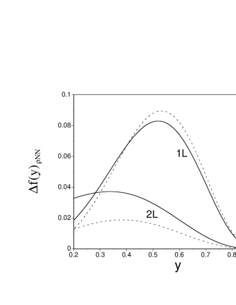
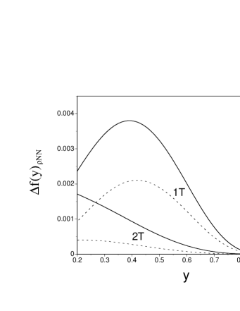
Figure 2: Meson momentum distributions $\Delta f_{1L}(y)$ and $\Delta f_{2L}(y)$ from the $\rho NN$ process. The solid and dashed curves are obtained at $Q^{2}$=1 and 2 GeV², respectively, with $x$=0.2. The isospin factors are taken out from the distributions as explained in the text.

Figure 3: Meson momentum distributions $\Delta f_{1T}(y)$ and $\Delta f_{2T}(y)$ from the $\rho NN$ process. The solid and dashed curves are obtained at $Q^{2}$=1 and 2 GeV², respectively, with $x$=0.2.

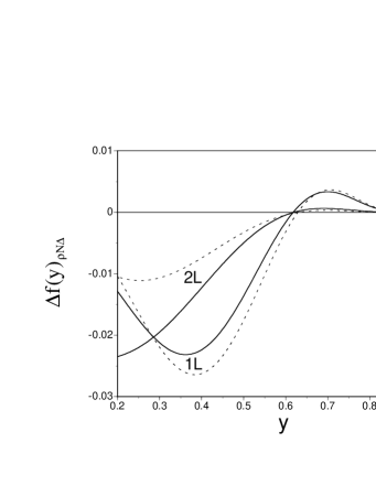
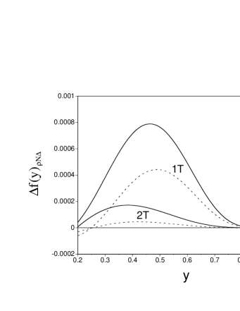
Figure 4: Meson momentum distributions $\Delta f_{1L}(y)$ and $\Delta f_{2L}(y)$ from the $\rho N\Delta$ process. The solid and dashed curves are obtained at $Q^{2}$=1 and 2 GeV², respectively, with $x$=0.2.

Figure 5: Meson momentum distributions $\Delta f_{1T}(y)$ and $\Delta f_{2T}(y)$ from the $\rho N\Delta$ process. The solid and dashed curves are obtained at $Q^{2}$=1 and 2 GeV², respectively, with $x$=0.2.

We show the numerical results in Figs. 3–5 for the vertex momentum (B), which is the preferred choice according to Ref. julich . In addition to the variable $y$, the distributions depend also on $x$ and $Q^{2}$. The distributions are calculated at $x=0.2$ with $Q^{2}$=1 and 2 GeV² for the solid and dashed curves, respectively. Because of the $x$ dependence, the unphysical region $y<x$ is not shown in these figures. In Figs. 3 and 3, the distributions due to the $\rho NN$ process are shown. In Figs. 5 and 5, the distributions due to the $\rho N\Delta$ process are shown. In these distributions, the isospin factors are taken out from the distributions, so that the distributions $\Delta f(y)/|\widetilde{\phi}_{V}^{*}\cdot\widetilde{T}|^{2}$ are actually shown, and there are differences of factors 3 (in $\rho NN$) and 2 (in $\rho N\Delta$) from those in Ref. fs . The coupling constants are taken as $g_{V}^{2}/(4\pi)=0.84$, $f_{V}=6.1g_{V}$, and $f_{VN\Delta}^{2}/(4\pi)=20.45$ mhe .

In spite of the positive $\Delta f_{1L}(y)$ and $\Delta f_{2L}(y)$ distributions from the $\rho NN$ process in Fig. 3, the distributions from the $\rho N\Delta$ are mainly negative. In the unpolarized case, the meson momentum distributions are, of course, positive. However, because the distribution $\Delta f(y)$ is defined by the helicity difference in Eq. (31), it becomes either positive or negative depending on the helicity structure at the $VNB$ vertex. For the meson angular momentum state $\ell_{z}$, the $VNB$ vertex amplitude is proportional to $k_{\perp}^{\ell_{z}}$ and higher order terms. Since the momentum $k_{\perp}$ is in general much smaller than the nucleon mass, the vertex amplitudes with $\ell_{z}=0$ contribute dominantly to $\Delta f(y)$. There is only one $\rho NN$ amplitude with $\ell_{z}=0$ and $\lambda_{V}\neq 0$, and it has the helicity structure $\lambda_{V}=+1$ and $\lambda_{N}^{\prime}=-1/2$, where the initial helicity is fixed at $\lambda_{N}=+1/2$. This fact indicates that $f_{1L}^{\lambda_{V}=+1}(y)$ and $f_{2L}^{\lambda_{V}=+1}(y)$ are certainly larger than $f_{1L}^{\lambda_{V}=-1}(y)$ and $f_{1L}^{\lambda_{V}=-1}(y)$, respectively, which results in the positive distributions $\Delta f_{1L}(y)$ and $\Delta f_{1L}(y)$ from the $\rho NN$ process. On the other hand, there are two amplitudes with $\ell_{z}=0$ and $\lambda_{V}\neq 0$ in the $\rho N\Delta$ process, and they have helicity states $\lambda_{V}=-1$, $\lambda_{\Delta}=+3/2$ and $\lambda_{V}=+1$, $\lambda_{\Delta}=-1/2$. Actually calculating these helicity amplitudes, we find that both amplitudes depend much on the momentum choice, namely (A) or (B), at the $\rho N\Delta$ vertex. Therefore, $f_{1L}^{\lambda_{V}=+1}(y)$ and $f_{2L}^{\lambda_{V}=+1}(y)$ are either larger or smaller than $f_{1L}^{\lambda_{V}=-1}(y)$ and $f_{2L}^{\lambda_{V}=-1}(y)$, respectively, depending on the momentum choice. In the prescription (B), the positive helicity distributions $f_{1L}^{\lambda_{V}=+1}(y)$ and $f_{2L}^{\lambda_{V}=+1}(y)$ are mostly smaller, so that $\Delta f_{1L}(y)$ and $\Delta f_{2L}(y)$ become negative distributions in the wide $x$ region. However, the situation is opposite in the prescription (A), where the distributions are mostly positive.

As expected, the distributions $\Delta f_{1L}(y)$ in Figs. 3 and 5 are the dominant ones and they are almost independent of $Q^{2}$. However, $\Delta f_{2L}(y)$, $\Delta f_{1T}(y)$, and $\Delta f_{2T}(y)$ are roughly proportional to $1/Q^{2}$, so that these new contributions become more important as $Q^{2}$ becomes smaller. Figures 3$-$5 clearly show this tendency. The transverse distributions $\Delta f_{1T}(y)$ and $\Delta f_{2T}(y)$ are an order of magnitude smaller than the longitudinal ones $\Delta f_{1L}(y)$ and $\Delta f_{2L}(y)$. Therefore, the major correction comes from the distribution $\Delta f_{2L}(y)$, which is almost comparable magnitude with $\Delta f_{1L}(y)$ in Figs. 3 and 5. Because the correction terms are proportional to $\gamma^{2}=4m_{N}^{2}x^{2}/Q^{2}$, they are small contributions in the kinematical range $x<0.05$ with $Q^{2}>$1 GeV². However, their effects become more pronounced as $x$ becomes larger.

IV Results

For calculating the $\Delta\bar{u}-\Delta\bar{d}$ distribution numerically, we need the polarized antiquark distributions in $\rho$, the isospin factors, and the vertex form factors. The $\rho$-meson parton distributions are not known, so that the same prescription is used as the one in Refs. fs ; cs . Considering a lattice QCD estimate lattice , the polarized valence-quark distribution is assumed as

$$\Delta V_{\rho}(x,Q^{2})=0.6\,V_{\pi}(x,Q^{2}),$$ (1)

at $Q^{2}$=1 GeV². The distribution in the pion is taken from the GRS (Glück, Reya, and Schienbein) parametrization in 1999 grs99 . The charge symmetry suggests the relation for the valence-quark distributions:

$$(\Delta\bar{u})_{\rho^{-}}^{val}=(\Delta\bar{d})_{\rho^{+}}^{val}=2(\Delta\bar{u})_{\rho^{0}}^{val}=2(\Delta\bar{d})_{\rho^{0}}^{val}=\Delta V_{\rho}.$$ (2)

For the sea-quark distributions, they are assumed to be flavor symmetric. Then, we obtain the $\Delta\bar{u}-\Delta\bar{d}$ distributions in the $\rho$ meson:

$$(\Delta\bar{u}-\Delta\bar{d})_{\rho^{+}} =-\Delta V_{\rho},$$

$$(\Delta\bar{u}-\Delta\bar{d})_{\rho^{0}} =0,$$

$$(\Delta\bar{u}-\Delta\bar{d})_{\rho^{-}} =+\Delta V_{\rho}.$$ (3)

For the $g_{2}$ part of $\rho$, the Wandzura-Wilczek relation is used as discussed in Sec. II:

$$\Delta V_{\rho}^{WW}(x,Q^{2})=-\Delta V_{\rho}(x,Q^{2})+\int_{x}^{1}\frac{dy}{y}\Delta V_{\rho}(y,Q^{2}).$$ (4)

Both the valence-quark distribution and the WW distribution are shown at $Q^{2}$=1 GeV² in Fig. 6.

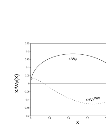
Figure 6: Assumed polarized valence-quark distribution in the $\rho$ meson and the WW distribution at $Q^{2}$=1 GeV².

Necessary isospin factors are calculated from Eq. (3) as

$$|\!<\!n\,|\,\widetilde{\phi}_{\rho^{+}}^{*}\!\cdot\widetilde{T}\,|\,p\!>\!|^{2} =2\,,$$

$$|\!<\!\Delta^{0}\,|\,\widetilde{\phi}_{\rho^{+}}^{*}\!\cdot\widetilde{T}\,|\,p\!>\!|^{2} =1/3\,,$$

$$|\!<\!\Delta^{++}\,|\,\widetilde{\phi}_{\rho^{-}}^{*}\!\cdot\widetilde{T}\,|\,p\!>\!|^{2} =1\,.$$ (5)

Using Eqs. (36), (3), and (5), we obtain

$$(\Delta \bar{u}-\Delta\bar{d})_{p\rightarrow\rho B}=\sum_{\rho,B}\bigg{[}\,\big{\{}\,\Delta f_{1L}+\Delta f_{1T}\,\big{\}}\otimes(\Delta\bar{u}-\Delta\bar{d})_{\rho}$$

$$\ \ \ \ \ \ \ \ \ \ \ \ \ \ \ \ -\big{\{}\,\Delta f_{2L}+\Delta f_{2T}\,\big{\}}\otimes(\Delta\bar{u}-\Delta\bar{d})_{\rho}^{WW}\,\bigg{]}$$

$$=\bigg{[}\,-2\,\Delta f^{\rho NN}_{1L+1T}+\frac{2}{3}\,\Delta f^{\rho N\Delta}_{1L+1T}\,\bigg{]}\otimes\Delta V_{\rho}$$

$$\ -\bigg{[}\,-2\,\Delta f^{\rho NN}_{2L+2T}+\frac{2}{3}\,\Delta f^{\rho N\Delta}_{2L+2T}\,\bigg{]}\otimes\Delta V_{\rho}^{WW}\,,$$ (6)

where $\otimes$ indicates the convolution integral in Eq. (36):

$$a\otimes b=\frac{1}{1+\gamma^{2}}\int_{x}^{1}\frac{dy}{y}\,a(y)\,b(x/y).$$ (7)

The meson momentum distributions $\Delta f^{\rho NN}_{1L+1T}$ and $\Delta f^{\rho NN}_{2L+2T}$ are defined by extracting the isospin factors:

$$\Delta f^{\rho NB}_{iL+iT}=\frac{\Delta f_{iL}+\Delta f_{iT}}{|\widetilde{\phi}_{\rho}^{*}\!\cdot\widetilde{T}|^{2}},\ \ \ \text{$i$=1, 2}.$$ (8)

The expression of Eq. (6) may seem to be different from Refs. fs ; cs even in the limit $Q^{2}\rightarrow\infty$; however, it is just the matter of the definition of the meson momentum distributions. They included the isospin factor

$$|\!<\!n\,|\,\widetilde{\phi}_{\rho^{+}}^{*}\!\cdot\widetilde{T}\,|\,p\!>\!|^{2}+|\!<\!p\,|\,\widetilde{\phi}_{\rho^{0}}^{*}\!\cdot\widetilde{T}\,|\,p\!>\!|^{2}=3\,,$$ (9)

in the distribution $\Delta f(y)$ for the $\rho NN$ process and the factor

$$|\!<\!\Delta^{0}\,|\,\widetilde{\phi}_{\rho^{+}}^{*}\!\cdot\widetilde{T}\, |\,p\!>\!|^{2}+|\!<\!\Delta^{+}\,|\,\widetilde{\phi}_{\rho^{0}}^{*}\!\cdot\widetilde{T}\,|\,p\!>\!|^{2}$$

$$+|\!<\!\Delta^{++}\,|\,\widetilde{\phi}_{\rho^{-}}^{*}\!\cdot\widetilde{T}\,|\,p\!>\!|^{2}=2$$ (10)

for the $\rho N\Delta$. Therefore, our expression certainly agrees on those in Refs. fs ; cs at $Q^{2}\rightarrow\infty$.

The remaining quantities are the vertex form factors. They are roughly known from the studies of one-boson-exchange potentials (OBEPs); however, a slight change of the cutoff parameter could result in a large difference of antiquark distributions. Furthermore, there is an issue of the charge and momentum conservations for the splitting process msm if a $t$ $(=(p_{N}-p_{B})^{2})$ dependent form factor is used. A possible solution is to use the $t$ dependent form factor multiplied by a $u$ dependent one zoller . For this purpose, it is more convenient to take an exponential form factor so as to become the additional form $t+u$ within the form factor:

$$F_{\rho NN}(k)=F_{\rho N\Delta}(k)=\exp\bigg{[}\frac{m_{N}^{2}-m_{VB}^{2}}{2\Lambda_{e}^{2}}\bigg{]},$$ (11)

where $m_{VB}^{2}$ is defined in Eq. (15), and the cutoff parameter $\Lambda_{e}$ is taken as $\Lambda_{e}$=1 GeV in the following numerical results. In Ref. julich , the cutoff parameters are obtained by fitting baryon-production cross sections $pp\rightarrow BX$: $\Lambda_{e}^{\rho NN}$=1.10 GeV and $\Lambda_{e}^{\rho N\Delta}$=0.98 GeV. However, the parameters are not well determined in general. We discuss the dependence on this cutoff value at the end of this section. The form factors are the same as the ones in the previous publications fs ; cs , so that we could compare our results with theirs.

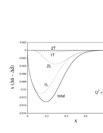
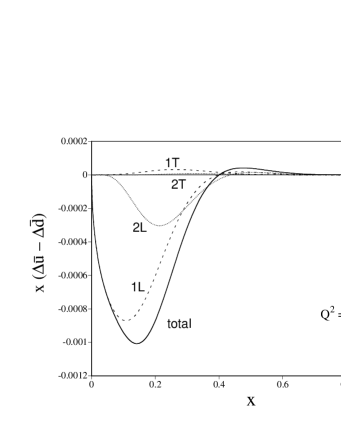
Figure 7: $\Delta\bar{u}-\Delta\bar{d}$ distributions from the $\rho NN$ process at $Q^{2}$=1 GeV². The $1L$, $2L$, $1T$, and $2T$ type contributions and their summation are shown.

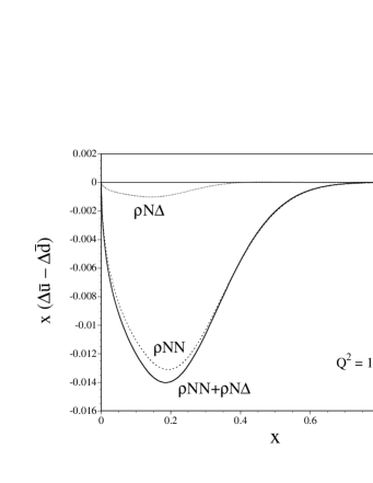
Figure 8: $\Delta\bar{u}-\Delta\bar{d}$ distributions from the $\rho N\Delta$ process at $Q^{2}$=1 GeV². The $1L$, $2L$, $1T$, and $2T$ type contributions and their summation are shown.

Figure 9: $\Delta\bar{u}-\Delta\bar{d}$ distributions from the $\rho NN$ and $\rho N\Delta$ processes at $Q^{2}$=1 GeV².

Using these form factors and the parton distributions in $\rho$, we obtain the $\rho NN$ and $\rho N\Delta$ process contributions to the $\Delta\bar{u}-\Delta\bar{d}$ in the nucleon. In Fig. 9, the $1L$, $2L$, $1T$, and $2T$ type distributions from the $\rho NN$ process are shown at $Q^{2}$=1 GeV² together with their total. The ordinary $1L$ term is the dominant contribution; however, the $2L$ term becomes important at $x>0.3$. It is as large as the $1L$ distribution in the medium $x$ region although it is fairly small at $x<0.05$. The $1T$ and $2T$ distributions are very small in the whole $x$ range. Because $p\rightarrow\rho^{+}n$ is the only contributing process in which the valence $\bar{d}$ distribution in $\rho^{+}$ plays the main role, the $\rho NN$ contributions are negative in the $\Delta\bar{u}-\Delta\bar{d}$ in the nucleon.

Each term contribution has almost the same tendency in the $\rho N\Delta$ process as shown in Fig. 9: the $1L$ term is the major one and the $2L$ term provides some corrections depending on the $x$ region. There are two contributing processes, $p\rightarrow\rho^{+}\Delta^{0}$ and $p\rightarrow\rho^{-}\Delta^{-}$, and the isospin factor is three times larger in the latter one. This fact may seem to indicate that the $\rho N\Delta$ processes provide a positive contribution to $\Delta\bar{u}-\Delta\bar{d}$ in the nucleon due to the valence $\bar{u}$ distribution in $\rho^{-}$. This kind of explanation is certainly valid in the unpolarized flavor asymmetry udsum ; skubdb . However, this is not the case in Fig. 9, where the $1L$ and $1T$ distributions are mostly negative. This misleading result comes from the helicity structure at the $N\rightarrow\rho\Delta$ vertex. Although the helicity difference $\Delta f(y)$ is positive for the $\rho NN$, it is negative for the $\rho N\Delta$ in the case (B) as explained in Sec. III. Therefore, the $\rho N\Delta$ contribution becomes also negative for the $\Delta\bar{u}-\Delta\bar{d}$ distribution.

Next, the $\rho NN$ and $\rho N\Delta$ contributions are compared in Fig. 9. The magnitude of the $\rho N\Delta$ contribution is very small compared with the $\rho NN$ one in (B). From Figs. 3 and 5, we find that the magnitude of $\Delta f^{\rho N\Delta}(y)$ is already three times smaller than $\Delta f^{\rho NN}(y)$, and the $\rho N\Delta$ contribution is further suppressed by the isospin factor (2/3)/2=1/3. Therefore, the overall magnitude becomes much smaller.

Figure 10: $\Delta\bar{u}-\Delta\bar{d}$ distributions from the $\rho NN$ and $\rho N\Delta$ processes at $Q^{2}$=1 GeV² for the vertex momentum choice (A).

As discussed in Sec. III, we may have another vertex choice (A) instead of (B). In showing the numerical results so far, the model (B) has been used. We show the choice (A) results in Fig. 10. It is obvious that the distributions depend much on this vertex choice. There are two major differences from Fig. 9. One is that the order of magnitude is much smaller in the $\rho NN$ distribution, and the other is that the $\rho N\Delta$ distribution becomes positive. These are due to the difference of helicity structure at the vertices between (A) and (B).

We also discuss the vertex cutoff dependence. The vertex cutoff has been taken as $\Lambda_{e}$=1 GeV in this section; however, it is well known that calculated antiquark distributions are very sensitive to the cutoff value skubdb . In the present paper, the exponential form factor is used instead of dipole or monopole form factor, which is more popular in the studies of OBEPs. The cutoff parameters of different form factors could be related by skubdb

$$\Lambda_{1}=0.62\Lambda_{2}=0.78\sqrt{2}\Lambda_{e},$$ (12)

where the monopole and dipole parameters are defined by the form factors

$$F^{(1)}_{VNB}(k)=\frac{1-m_{N}^{2}/\Lambda_{1}^{2}}{1-m_{VB}^{2}/\Lambda_{1}^{2}},\ \ F^{(2)}_{VNB}(k)=\frac{(1-m_{N}^{2}/\Lambda_{2}^{2})^{2}}{(1-m_{VB}^{2}/\Lambda_{2}^{2})^{2}}.$$ (13)

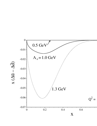
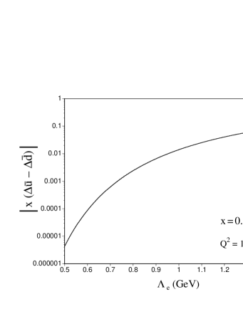
Figure 11: Cutoff dependence of $\Delta\bar{u}-\Delta\bar{d}$ is shown at $Q^{2}$=1 GeV² by taking $\Lambda_{e}$=0.5, 1.0, and 1.3 GeV.

Figure 12: Cutoff dependence of $|\Delta\bar{u}-\Delta\bar{d}|$ is shown at $x=0.2$ and $Q^{2}$=1 GeV² as a function of the parameter $\Lambda_{e}$.

Even in the well investigated pion-nucleon coupling, the monopole cutoff parameter $\Lambda_{1}$ ranges from 0.6 GeV to 1.4 GeV in quark models and OBEPs skubdb . It roughly corresponds to $\Lambda_{e}$ from 0.5 GeV to 1.3 GeV according to Eq. (12). We show the $\Delta\bar{u}-\Delta\bar{d}$ distributions for various cutoff parameters, $\Lambda_{e}$=0.5, 1.0, and 1.3 GeV in Fig. 12 for the prescription (B). In the unpolarized distribution $\bar{u}-\bar{d}$ in Ref. skubdb , it is fortunate that the cutoff dependence is rather small because of the cancellation between the $\pi NN$ and $\pi N\Delta$ processes. However, the $\rho NN$ is the dominant contribution, as shown in Fig. 9, in the present polarized studies of (B), so that the overall magnitude is much dependent on the cutoff parameter. There are orders of magnitude differences between the three curves. Next, fixing $x$ at 0.2, we show the cutoff dependence in Fig. 12. In fact, there is four orders of magnitude variation from $\Lambda_{e}$=0.5 to 1.5 GeV. Therefore, an accurate determination of the cutoff parameters is a key for a reliable meson-cloud prediction.

There have been studies in chiral soliton models models . They predict very different distributions, namely $\Delta\bar{u}$ excess over $\Delta\bar{d}$ and the order of magnitude of $\Delta\bar{u}-\Delta\bar{d}$ is large ($\sim 0.4$) at $x$=0.2. Although the soliton models and the meson-cloud models obtain very similar distributions for the unpolarized $\bar{u}-\bar{d}$, it is interesting to find opposite prediction for the polarized distributions. The physics reason for the difference is not clear at this stage. In any case, the distribution $\Delta\bar{u}-\Delta\bar{d}$ should be clarified experimentally in the near future by $W$ production process rhic and semi-inclusive experiments compass . Furthermore, there is a possibility to use the polarized proton-deuteron Drell-Yan process pddy in combination with the proton-proton reaction. Until the data will be taken, the theoretical predictions should be discussed in details for comparison.

V Conclusions

The $\rho$ meson contributions to the polarized antiquark distribution $\Delta\bar{u}-\Delta\bar{d}$ have been investigated. In particular, we pointed out that the $g_{2}$ part of $\rho$ contributes to the polarized distributions in the nucleon. We obtained the extra contributions denoted as $2L$, $1T$, and $2T$ in addition to the ordinary one ($1L$). Although the extra terms are small in the small $x$ region ($x<0.05$), the magnitude of the $2L$ term becomes comparable to the ordinary one in the $x$ region $x>0.2$. The $g_{2}^{\rho}$ contributions are important in the kinematical region of medium $x$ with small $Q^{2}$. The obtained $\Delta\bar{u}-\Delta\bar{d}$ is very sensitive to the cutoff parameter. The model should be investigated further in order to compare with future experimental data.

Appendix A Analytical expressions of meson momentum distributions

In the limit $Q^{2}\rightarrow\infty$, the following meson momentum distributions agree on those by Fries and Schäfer (FS) fs with a minor misprint in a $\rho N\Delta$ term. The situation of the momentum distributions is somewhat confusing in the sense that Cao and Signal (CS) cs pointed out two major differences from Ref. fs although the formalism is exactly the same except for interference terms. According to Ref. cs , all the $g_{\rho NN}f_{\rho NN}$ ($g_{v}f_{v}$ in our notation) terms should be replaced by $-g_{\rho NN}f_{\rho NN}$, and the momentum (B) results for $\rho N\Delta$ agree on those of (A) in Ref. fs instead of (B).

In spite of their claim, we believe that the FS results are right with the following reasons. We also checked the helicity amplitudes in Ref. julich , which is referred to as Jülich in the following. In addition to obvious typos, our results differ from the Jülich expressions. First, complex conjugate should be taken if their expressions are given for the process $N\rightarrow\rho B$ as indicated in their appendix. Second, $f_{v}$ terms have different sign. If the Jülich amplitudes were written for $N\rho\rightarrow B$ or $B\rightarrow\rho N$, we would agree on their expressions. Depending on the $\rho$ momentum direction, the $f_{v}$ term in Eq. (1) becomes either positive or negative, which could lead to the different sign of the $g_{v}f_{v}$ terms. However, it is obvious that the outgoing meson is considered in the formalism. Furthermore, taking summations of the helicity amplitudes, we reproduce the unpolarized momentum distributions of Melnitchouk and Thomas mt ; fries , whereas the CS results are inconsistent. The $VNN$ vertex in Eq. (1) is also consistent with the one in Ref. mach86 .

We also tested $\rho N\Delta$ helicity amplitudes in the vertex momentum (B), but the results disagree on the Jülich expressions. However, if the momentum (A) is used, our results agree on them. It seems to us that the helicity amplitudes are shown for the choice (B) in $\rho NN$ and for (A) in $\rho N\Delta$. Therefore, as far as we investigated, we believe that the FS calculations are right also for the $\rho N\Delta$ process.

In the following, we show the helicity dependent meson momentum distributions. Because the distributions with $\lambda_{V}=0$ are irrelevant for calculating $\Delta f(y)$, so that they are not shown. The isospin factors are extracted out from the expressions.

$$f^{\lambda_{V}}_{1L,\,VNB}\,(y)=\int_{0}^{(\vec{k}_{\perp}^{\,2})_{max}}\frac{dk_{\perp}^{2}}{16\pi^{2}}\frac{F^{2}_{VNB}\,({y^{\prime}},\,k_{\perp}^{2})}{\left\{m_{N}^{2}-m_{VB}^{2}\,({y^{\prime}},\,k_{\perp}^{2})\right\}^{2}}$$

$$\ \ \times\frac{\partial{y^{\prime}}}{\partial y}\,\frac{y}{{y^{\prime}}}\left\{1+\frac{k_{\perp}^{2}}{y{y^{\prime}}m_{N}^{2}}(\sqrt{1+\gamma^{2}}-1)\right\}\,D^{L,\,\lambda_{V}}_{VNB}\,({y^{\prime}},\,k_{\perp}^{2})\ ,$$ (1)

$$f^{\lambda_{V}}_{1T,\,VNB}\,(y)=\int_{0}^{(\vec{k}_{\perp}^{\,2})_{max}}\frac{dk_{\perp}^{2}}{16\pi^{2}}\frac{F^{2}_{VNB}\,({y^{\prime}},\,k_{\perp}^{2})}{\left\{m_{N}^{2}-m_{VB}^{2}\,({y^{\prime}},\,k_{\perp}^{2})\right\}^{2}}$$

$$\ \ \times\frac{\partial{y^{\prime}}}{\partial y}\,\frac{y}{{y^{\prime}}}\,\gamma^{2}\,\frac{k_{\perp}}{2ym_{N}}\,D^{T,\,\lambda_{V}}_{VNB}\,({y^{\prime}},\,k_{\perp}^{2})\ ,$$ (2)

$$f^{\lambda_{V}}_{2L,\,VNB}\,(y)=\int_{0}^{(\vec{k}_{\perp}^{\,2})_{max}}\frac{dk_{\perp}^{2}}{16\pi^{2}}\frac{F^{2}_{VNB}\,({y^{\prime}},\,k_{\perp}^{2})}{\left\{m_{N}^{2}-m_{VB}^{2}\,({y^{\prime}},\,k_{\perp}^{2})\right\}^{2}}$$

$$\ \ \times\frac{\partial{y^{\prime}}}{\partial y}\,\frac{y}{{y^{\prime}}}\,\gamma^{2}\,\frac{m_{V}^{2}}{y^{2}m_{N}^{2}}\,D^{L,\,\lambda_{V}}_{VNB}\,({y^{\prime}},\,k_{\perp}^{2})\ ,$$ (3)

$$f^{\lambda_{V}}_{2T,\,VNB}\,(y)=\int_{0}^{(\vec{k}_{\perp}^{\,2})_{max}}\frac{dk_{\perp}^{2}}{16\pi^{2}}\frac{F^{2}_{VNB}\,({y^{\prime}},\,k_{\perp}^{2})}{\left\{m_{N}^{2}-m_{VB}^{2}\,({y^{\prime}},\,k_{\perp}^{2})\right\}^{2}}$$

$$\ \ \times\frac{\partial{y^{\prime}}}{\partial y}\,\frac{y}{{y^{\prime}}}\,\gamma^{2}\,\frac{k_{\perp}m_{V}^{2}}{2y^{2}{y^{\prime}}m_{N}^{3}}(\sqrt{1+\gamma^{2}}-1)\,D^{T,\,\lambda_{V}}_{VNB}\,({y^{\prime}},\,k_{\perp}^{2})\ .$$ (4)

Here, the partial derivative is given by

$$\frac{\partial{y^{\prime}}}{\partial y}\,\frac{y}{{y^{\prime}}}=\left\{1+\frac{\gamma^{2}}{y^{2}m_{N}^{2}}(k_{\perp}^{2}+m_{V}^{2})\right\}^{-1/2}.$$ (5)

The distributions $D^{L,\,\lambda_{V}}_{VNN}\,({y^{\prime}},\,k_{\perp}^{2})$ are calculated for the prescription (A) as

$$D^{L,\,+1}_{VNN}\,({y^{\prime}},\,k_{\perp}^{2})=\frac{2}{y^{\prime{3}}(1-{y^{\prime}})^{2}}\,\bigg{[}\,g_{V}^{2}\left(k_{\perp}^{2}+y^{\prime{4}}m_{N}^{2}\right)$$

$$\ \ +g_{V}f_{V}{y^{\prime}}\left[k_{\perp}^{2}+{y^{\prime}}\left\{y^{\prime{2}}m_{N}^{2}-(1-{y^{\prime}})m_{V}^{2}\right\}\right]$$

$$\ \ +\frac{f_{V}^{2}}{4m_{N}^{2}}\left[y^{\prime{2}}m_{N}^{2}k_{\perp}^{2}+\left\{y^{\prime{2}}m_{N}^{2}-(1-{y^{\prime}})m_{V}^{2}\right\}^{2}\right]\bigg{]}\,,$$ (6)

$$D^{L,\,-1}_{VNN}\,({y^{\prime}},\,k_{\perp}^{2})=\frac{2k_{\perp}^{2}}{y^{\prime{3}}(1-{y^{\prime}})^{2}}\,\bigg{[}\,g_{V}^{2}(1-{y^{\prime}})^{2}$$

$$\ \ -g_{V}f_{V}{y^{\prime}}(1-{y^{\prime}})+\frac{f_{V}^{2}}{4m_{N}^{2}}\left(k_{\perp}^{2}+y^{\prime{2}}m_{N}^{2}\right)\bigg{]}\,,$$ (7)

$$D^{T,\,\lambda_{V}}_{VNN}\,({y^{\prime}},\,k_{\perp}^{2})=\frac{\lambda_{V}k_{\perp}}{y^{\prime{3}}(1-{y^{\prime}})^{2}}\,\bigg{[}\,-2g_{V}^{2}y^{\prime{2}}(1-{y^{\prime}})m_{N}$$

$$\ \ +\frac{g_{V}f_{V}}{m_{N}}\left\{k_{\perp}^{2}-y^{\prime{2}}(1-2{y^{\prime}})m_{N}^{2}+(1-{y^{\prime}})^{2}m_{V}^{2}\right\}$$

$$\ \ +\frac{f_{V}^{2}}{4m_{N}^{2}}2{y^{\prime}}m_{N}\left\{k_{\perp}^{2}+y^{\prime{2}}m_{N}^{2}-(1-{y^{\prime}})m_{V}^{2}\right\}\bigg{]}\,.$$ (8)

In the $VN\Delta$ process, the distributions are calculated for the vertex momentum (A) as

$$D^{L,\,+1}_{VN\Delta}\,({y^{\prime}},\,k_{\perp}^{2})=\frac{f_{VN\Delta}^{2}}{3y^{\prime{3}}(1-{y^{\prime}})^{4}m_{\Delta}^{2}m_{V}^{2}}\,$$

$$\ \ \times\bigg{[}\,k_{\perp}^{6}+k_{\perp}^{4}\left\{3-4{y^{\prime}}(1-{y^{\prime}})\right\}m_{\Delta}^{2}$$

$$\ \ +k_{\perp}^{2}\Big{[}y^{\prime{2}}\left\{2y^{\prime{2}}+(2-{y^{\prime}})^{2}\right\}m_{\Delta}^{4}$$

$$\ \ +4{y^{\prime}}(1-{y^{\prime}})^{3}m_{N}m_{\Delta}m_{V}^{2}\Big{]}+y^{\prime{4}}m_{\Delta}^{6}$$

$$\ \ -2y^{\prime{2}}(1-{y^{\prime}})^{3}m_{N}m_{\Delta}^{3}m_{V}^{2}+(1-{y^{\prime}})^{6}m_{N}^{2}m_{V}^{4}\bigg{]}\,,$$ (9)

$$D^{L,\,-1}_{VN\Delta}\,({y^{\prime}},\,k_{\perp}^{2})=\frac{f_{VN\Delta}^{2}}{3y^{\prime{3}}(1-{y^{\prime}})^{2}m_{\Delta}^{2}m_{V}^{2}}\,$$

$$\ \ \times\bigg{[}\,k_{\perp}^{4}m_{N}^{2}+k_{\perp}^{2}\{4y^{\prime{2}}m_{N}^{2}m_{\Delta}^{2}-4{y^{\prime}}(1-{y^{\prime}})m_{N}m_{\Delta}m_{V}^{2}$$

$$\ \ +(1-{y^{\prime}})^{2}m_{V}^{4}\}+3y^{\prime{4}}m_{N}^{2}m_{\Delta}^{4}-6y^{\prime{2}}(1-{y^{\prime}})m_{N}m_{\Delta}^{3}m_{V}^{2}$$

$$\ \ +3(1-{y^{\prime}})^{2}m_{\Delta}^{2}m_{V}^{4}\bigg{]}\,,$$ (10)

$$D^{T,\,\lambda_{V}}_{VN\Delta}\,({y^{\prime}},\,k_{\perp}^{2})=\frac{\lambda_{V}f_{VN\Delta}^{2}k_{\perp}}{3y^{\prime{3}}(1-{y^{\prime}})^{3}m_{\Delta}^{2}m_{V}^{2}}\,\bigg{[}\,k_{\perp}^{4}m_{N}$$

$$\ \ -2{y^{\prime}}k_{\perp}^{2}\left\{(1-2{y^{\prime}})m_{N}m_{\Delta}^{2}+(1-{y^{\prime}})m_{\Delta}m_{V}^{2}\right\}$$

$$\ \ -(2-3{y^{\prime}})y^{\prime{3}}m_{N}m_{\Delta}^{4}-2y^{\prime{2}}(1-{y^{\prime}})m_{\Delta}^{3}m_{V}^{2}$$

$$\ \ +2{y^{\prime}}(1-{y^{\prime}})^{3}m_{N}^{2}m_{\Delta}m_{V}^{2}-(1-{y^{\prime}})^{4}m_{N}m_{V}^{4}\bigg{]}\,.$$ (11)

In the same way, the distributions are obtained for the prescription (B) as

$$D^{L,\,+1}_{VNN}\,({y^{\prime}},\,k_{\perp}^{2})=\frac{2}{y^{\prime{3}}(1-{y^{\prime}})^{2}}\,\bigg{[}\,g_{V}^{2}\left(k_{\perp}^{2}+y^{\prime{4}}m_{N}^{2}\right)$$

$$\ \ +g_{V}f_{V}{y^{\prime}}\left\{(1+{y^{\prime}})k_{\perp}^{2}+2y^{\prime{3}}m_{N}^{2}\right\}$$

$$\ \ +\frac{f_{V}^{2}}{4m_{N}^{2}}\left(k_{\perp}^{2}+y^{\prime{2}}m_{N}^{2}\right)\left(k_{\perp}^{2}+4y^{\prime{2}}m_{N}^{2}\right)\bigg{]}\,,$$ (12)

$$D^{L,\,-1}_{VNN}\,({y^{\prime}},\,k_{\perp}^{2})=\frac{2k_{\perp}^{2}}{y^{\prime{3}}(1-{y^{\prime}})^{2}}\,\bigg{[}\,g_{V}^{2}(1-{y^{\prime}})^{2}$$

$$\ \ -g_{V}f_{V}{y^{\prime}}(1-{y^{\prime}})+\frac{f_{V}^{2}}{4m_{N}^{2}}\left(k_{\perp}^{2}+y^{\prime{2}}m_{N}^{2}\right)\bigg{]}\,,$$ (13)

$$D^{T,\,\lambda_{V}}_{VNN}\,({y^{\prime}},\,k_{\perp}^{2})=\frac{\lambda_{V}k_{\perp}}{y^{\prime{3}}(1-{y^{\prime}})^{2}}\,\bigg{[}\,-2g_{V}^{2}y^{\prime{2}}(1-{y^{\prime}})m_{N}$$

$$\ \ +\frac{g_{V}f_{V}}{m_{N}}{y^{\prime}}\left\{k_{\perp}^{2}-(2-3{y^{\prime}}){y^{\prime}}m_{N}^{2}\right\}$$

$$\ \ +\frac{f_{V}^{2}}{4m_{N}^{2}}4{y^{\prime}}m_{N}\left\{k_{\perp}^{2}+y^{\prime{2}}m_{N}^{2}\right\}\bigg{]}\,,$$ (14)

$$D^{L,\,+1}_{VN\Delta}\,({y^{\prime}},\,k_{\perp}^{2})=\frac{f_{VN\Delta}^{2}}{3y^{\prime{3}}(1-{y^{\prime}})^{4}m_{\Delta}^{2}m_{V}^{2}}\,\bigg{[}\,k_{\perp}^{6}$$

$$\ \ +k_{\perp}^{4}\left\{(3-4{y^{\prime}}+4y^{\prime{2}})m_{\Delta}^{2}\right.-4{y^{\prime}}(1-{y^{\prime}})^{2}m_{N}m_{\Delta}$$

$$\ \ \left.+(1-{y^{\prime}})^{4}m_{N}^{2}\right\}+k_{\perp}^{2}\left\{y^{\prime{2}}(4-4{y^{\prime}}+3y^{\prime{2}})m_{\Delta}^{4}\right.$$

$$\ \ -2y^{\prime{2}}(1-{y^{\prime}})^{2}m_{N}m_{\Delta}^{3}+2{y^{\prime}}(1-{y^{\prime}})^{4}m_{N}^{2}m_{\Delta}^{2}$$

$$\ \ +4y^{\prime{2}}(1-{y^{\prime}})^{3}m_{N}^{3}m_{\Delta}-\left.2{y^{\prime}}(1-{y^{\prime}})^{5}m_{N}^{4}\right\}+y^{\prime{4}}m_{\Delta}^{6}$$

$$\ \ +2y^{\prime{3}}(1-{y^{\prime}})^{2}m_{N}m_{\Delta}^{5}+y^{\prime{2}}(1-{y^{\prime}})^{4}m_{N}^{2}m_{\Delta}^{4}$$

$$\ \ -2y^{\prime{3}}(1-{y^{\prime}})^{3}m_{N}^{3}m_{\Delta}^{3}-2y^{\prime{2}}(1-{y^{\prime}})^{5}m_{N}^{4}m_{\Delta}^{2}$$

$$\ \ +y^{\prime{2}}(1-{y^{\prime}})^{6}m_{N}^{6}\bigg{]}\,,$$ (15)

$$D^{L,\,-1}_{VN\Delta}\,({y^{\prime}},\,k_{\perp}^{2})=\frac{f_{VN\Delta}^{2}}{3y^{\prime{3}}(1-{y^{\prime}})^{2}m_{\Delta}^{2}m_{V}^{2}}\,\bigg{[}\,k_{\perp}^{6}$$

$$\ \ +k_{\perp}^{4}\left\{(3+2{y^{\prime}})m_{\Delta}^{2}\right.+\left.4{y^{\prime}}m_{N}m_{\Delta}+(1-2{y^{\prime}}+2y^{\prime{2}})m_{N}^{2}\right\}$$

$$\ \ +k_{\perp}^{2}\left\{{y^{\prime}}(6+{y^{\prime}})m_{\Delta}^{4}+10y^{\prime{2}}m_{N}m_{\Delta}^{3}\right.$$

$$\ \ -2{y^{\prime}}(3-4{y^{\prime}}-y^{\prime{2}})m_{N}^{2}m_{\Delta}^{2}-4y^{\prime{2}}(1-{y^{\prime}})m_{N}^{3}m_{\Delta}$$

$$\ \ +\left.y^{\prime{2}}(1-{y^{\prime}})^{2}m_{N}^{4}\right\}+3y^{\prime{2}}m_{\Delta}^{6}+6y^{\prime{3}}m_{N}m_{\Delta}^{5}$$

$$\ \ -3y^{\prime{2}}(2-2{y^{\prime}}-y^{\prime{2}})m_{N}^{2}m_{\Delta}^{4}-6y^{\prime{3}}(1-{y^{\prime}})m_{N}^{3}m_{\Delta}^{3}$$

$$\ \ +3y^{\prime{2}}(1-{y^{\prime}})^{2}m_{N}^{4}m_{\Delta}^{2}\bigg{]}\,,$$ (16)

$$D^{T,\,\lambda_{V}}_{VN\Delta}\,({y^{\prime}},\,k_{\perp}^{2})=\frac{\lambda_{V}f_{VN\Delta}^{2}k_{\perp}}{3y^{\prime{2}}(1-{y^{\prime}})^{3}m_{\Delta}^{2}m_{V}^{2}}$$

$$\ \ \times\bigg{[}\,k_{\perp}^{4}\left\{2m_{\Delta}+(2-{y^{\prime}})m_{N}\right\}+k_{\perp}^{2}\left\{4{y^{\prime}}m_{\Delta}^{3}\right.$$

$$\ \ -2(2-4{y^{\prime}}+y^{\prime{2}})m_{N}m_{\Delta}^{2}-2(1-{y^{\prime}})m_{N}^{2}m_{\Delta}$$

$$\ \ \left.+2(1-{y^{\prime}})^{3}m_{N}^{3}\right\}+2y^{\prime{2}}m_{\Delta}^{5}-{y^{\prime}}(1-2y^{\prime{2}})m_{N}m_{\Delta}^{4}$$

$$\ \ -2{y^{\prime}}(1-{y^{\prime}})m_{N}^{2}m_{\Delta}^{3}+2{y^{\prime}}(1-{y^{\prime}})^{3}m_{N}^{3}m_{\Delta}^{2}$$

$$\ \ +2{y^{\prime}}(1-{y^{\prime}})^{3}m_{N}^{4}m_{\Delta}-{y^{\prime}}(1-{y^{\prime}})^{4}m_{N}^{5}\bigg{]}\,.$$ (17)

The longitudinal distributions agree on the FS results in the limit $Q^{2}\rightarrow\infty$ except for a term in Eq. (16). The factor $1/y^{\prime{3}}(1-{y^{\prime}})^{2}$ is written as $1/y^{\prime{2}}(1-{y^{\prime}})^{3}$ in Ref. fs . It is possibly a misprint fries .

References

(1) New Muon Collaboration, P. Amaudruz et al.,
Phys. Rev. Lett. 66, 2712 (1991);
M. Arneodo et al., Phys. Rev. D50, R1 (1994).
(2) CERN-NA51 Collaboration,
A. Baldit et al., Phys. Lett. B332, 244 (1994).
(3) Fermilab-E866/NuSea Collaboration,
E. A. Hawker et al.,
Phys. Rev. Lett. 80, 3715 (1998);
J. C. Peng et al.,
Phys. Rev. D58, 092004 (1998);
R. S. Towell et al.,
Phys. Rev. D64, 052002 (2001).
(4) HERMES Collaboration, K. Ackerstaff et al.,
Phys. Rev. Lett. 81, 5519 (1998).
(5) S. Kumano, Phys. Rep. 303, 183 (1998);
J.-C. Peng and G. T. Garvey,
in Trend in Particle and Nuclear Physics,
Volume 1, Plenum Press (1999).
(6) F. Buccella and J. Soffer,
Mod. Phys. Lett. A8, 225 (1993);
D. Diakonov et al., Nucl. Phys. B480, 341 (1996);
Phys. Rev. D56, 4069 (1997);
B. Dressler et al.,
Eur. Phys. J. C14, 147 (2000);
M. Wakamatsu and T. Kubota,
Phys. Rev. D60, 034020 (1999);
M. Wakamatsu and T. Watabe,
Phys.Rev. D62, 017506 (2000):
R. S. Bhalerao, Phys. Rev. C63, 025208 (2001).
(7) R. J. Fries and A. Schäfer,
Phys. Lett. B443, 40 (1998).