Thermal fluctuations in the interacting pion gas

Abstract

We derive the two-particle fluctuation correlator in a thermal gas of $\pi$-mesons to the lowest order in an interaction due to a resonance exchange. A diagrammatic technique is used. We discuss how this result can be applied to event-by-event fluctuations in heavy-ion collisions, in particular, to search for the critical point of QCD. As a practical example, we determine the shape of the rapidity correlator.

I Introduction

The goal of heavy-ion collision experiments is to shed light on thermodynamic properties of strongly interacting matter and to determine the phase diagram of Quantum Chromodynamics (QCD). Recently, experimental [1, 2, 3] and theoretical [4, 5, 6, 7, 8, 9, 10, 11, 12, 13, 14, 15, 16, 17, 18, 19, 20, 21] study of event-by-event fluctuations has attracted interest, in particular, because these fluctuations carry information about QCD thermodynamics. Recent experimental data from RHIC and CERN SPS [2, 3] show non-trivial pattern of fluctuations which awaits theoretical understanding.

Thermodynamic description of the final stage of the heavy-ion collision is motivated, to a large extent, by a remarkable phenomenological success of statistical thermal model in describing the observed particle spectra [22]. As far as the fluctuations are concerned, the observed fluctuations are Gaussian to a very good approximation, and are consistent with being largely of thermodynamic origin (see [7] for more quantitative analysis). In this paper we shall not discuss the relationship between the thermodynamic and observed fluctuations in heavy-ion collisions in detail (in particular, we shall not discuss possible importance of non-equilibrium effects — see, e.g., [23]). At temperatures of order 120 MeV characteristic of the final stage (freezeout) of a high-energy heavy-ion collision, hot QCD is, to a good approximation, a gas of predominantly pions interacting through exchange of resonances. This motivates the main goal of this paper: to calculate equilibrium thermodynamic fluctuations given the interaction of pions.

The most interesting application of our results is the search for the critical point of QCD. As discussed in [6, 7], such a point is characterized by a divergent correlation length, i.e., a massless excitation, in the channel with the quantum numbers of the sigma meson (scalar isoscalar). The strategy of the search is to scan the QCD phase diagram by varying experimental parameters, such as the energy of the collision, looking for the signatures of the critical point [6, 7]. The fluctuations of pions are sensitive to the presence of light sigma excitation because of the direct coupling of pions and sigma: $\sigma\pi\pi$. Thus, measuring the pion fluctuations one could determine if the freezeout is occuring near the critical point [7].

Another important application of our results is the study of charge fluctuations [12, 13, 14, 15, 16, 17].

The purpose of the paper is more generic. We wish to derive a formula for the pion fluctuations, specifically, for the two-pion correlator, given the effective interactions of pions. We shall discuss in detail the effect of the interaction induced by the sigma exchange, both because of its application to the search for the critical point and because this interaction is the simplest. It is relatively straightforward to generalize the analysis and the results to interactions induced by exchanges of other resonances, such as $\rho$-meson.

The goal of this paper is to motivate and derive formulas such as (18). As a simple example of an application of these results we determine the rapidity correlator (22). Other applications and a detailed comparison of these results to experiment are deferred to further work.

II Two-particle correlator and fluctuations

Most of the commonly used fluctuation measures, such as Gaussian widths of event-by-event distributions of mean transverse momenta, $\langle(\Delta p_{T})^{2}\rangle$, or correlation coefficients such as, e.g., $\langle\Delta p_{T}\Delta N\rangle$ ($\Delta N$ is the multiplicity fluctuation), can be related to the two-particle correlator, or the two-particle momentum space density, as emphasized in [7, 9]. For completeness, and to underline the importance of the two-particle correlator, we shall repeat some typical relationships here. An expert may wish to skip this section.

Let us denote by $\langle\ldots\rangle$ an average over events. Let us assume that we binned the phase space into bins labeled by the values of momenta $\textstyle p$ (or $\textstyle k$). We denote by $n_{\mathchoice{{\hbox{\boldmath$\displaystyle p$}}}{{\hbox{\boldmath$\textstyle p$}}}{{\hbox{\boldmath$\scriptstyle p$}}}{{\hbox{\boldmath$\scriptscriptstyle p$}}}}$ the occupation number of a given bin in a given event. Then $\Delta n_{\mathchoice{{\hbox{\boldmath$\displaystyle p$}}}{{\hbox{\boldmath$\textstyle p$}}}{{\hbox{\boldmath$\scriptstyle p$}}}{{\hbox{\boldmath$\scriptscriptstyle p$}}}}\equiv n_{\mathchoice{{\hbox{\boldmath$\displaystyle p$}}}{{\hbox{\boldmath$\textstyle p$}}}{{\hbox{\boldmath$\scriptstyle p$}}}{{\hbox{\boldmath$\scriptscriptstyle p$}}}}-\langle n_{\mathchoice{{\hbox{\boldmath$\displaystyle p$}}}{{\hbox{\boldmath$\textstyle p$}}}{{\hbox{\boldmath$\scriptstyle p$}}}{{\hbox{\boldmath$\scriptscriptstyle p$}}}}\rangle$ is the fluctuation, in a given event, of this occupation number around the all-event mean. The two-point fluctuation correlator which will be discussed and calculated in this paper is then given by

$$\langle\Delta n_{\mathchoice{{\hbox{\boldmath$\displaystyle p$}}}{{\hbox{\boldmath$\textstyle p$}}}{{\hbox{\boldmath$\scriptstyle p$}}}{{\hbox{\boldmath$\scriptscriptstyle p$}}}}\,\Delta n_{\mathchoice{{\hbox{\boldmath$\displaystyle k$}}}{{\hbox{\boldmath$\textstyle k$}}}{{\hbox{\boldmath$\scriptstyle k$}}}{{\hbox{\boldmath$\scriptscriptstyle k$}}}}\rangle.$$ (1)

For example, the event-by-event fluctuation of the mean transverse momentum is related to the correlator (1):

$$\langle(\Delta p_{T})^{2}\rangle={1\over\langle N\rangle^{2}}\sum_{\mathchoice{{\hbox{\boldmath$\displaystyle p$}}}{{\hbox{\boldmath$\textstyle p$}}}{{\hbox{\boldmath$\scriptstyle p$}}}{{\hbox{\boldmath$\scriptscriptstyle p$}}}}\sum_{\mathchoice{{\hbox{\boldmath$\displaystyle k$}}}{{\hbox{\boldmath$\textstyle k$}}}{{\hbox{\boldmath$\scriptstyle k$}}}{{\hbox{\boldmath$\scriptscriptstyle k$}}}}\langle\Delta n_{\mathchoice{{\hbox{\boldmath$\displaystyle p$}}}{{\hbox{\boldmath$\textstyle p$}}}{{\hbox{\boldmath$\scriptstyle p$}}}{{\hbox{\boldmath$\scriptscriptstyle p$}}}}\,\Delta n_{\mathchoice{{\hbox{\boldmath$\displaystyle k$}}}{{\hbox{\boldmath$\textstyle k$}}}{{\hbox{\boldmath$\scriptstyle k$}}}{{\hbox{\boldmath$\scriptscriptstyle k$}}}}\rangle(p_{T}-\overline{p_{T}})(k_{T}-\overline{p_{T}}),$$ (2)

where $\overline{p_{T}}$ is the inclusive mean transverse momentum. Similarly, the correlator of $p_{T}$ and multiplicity fluctuations (also known as linear correlation coefficient), can be expressed as

$$\langle\Delta p_{T}\Delta N\rangle={1\over\langle N\rangle}\sum_{\mathchoice{{\hbox{\boldmath$\displaystyle p$}}}{{\hbox{\boldmath$\textstyle p$}}}{{\hbox{\boldmath$\scriptstyle p$}}}{{\hbox{\boldmath$\scriptscriptstyle p$}}}}\sum_{\mathchoice{{\hbox{\boldmath$\displaystyle k$}}}{{\hbox{\boldmath$\textstyle k$}}}{{\hbox{\boldmath$\scriptstyle k$}}}{{\hbox{\boldmath$\scriptscriptstyle k$}}}}\langle\Delta n_{\mathchoice{{\hbox{\boldmath$\displaystyle p$}}}{{\hbox{\boldmath$\textstyle p$}}}{{\hbox{\boldmath$\scriptstyle p$}}}{{\hbox{\boldmath$\scriptscriptstyle p$}}}}\,\Delta n_{\mathchoice{{\hbox{\boldmath$\displaystyle k$}}}{{\hbox{\boldmath$\textstyle k$}}}{{\hbox{\boldmath$\scriptstyle k$}}}{{\hbox{\boldmath$\scriptscriptstyle k$}}}}\rangle(p_{T}-\overline{p_{T}}).$$ (3)

The multiplicity fluctuation is related to (1) by an obvious formula:

$$\langle(\Delta N)^{2}\rangle=\sum_{\mathchoice{{\hbox{\boldmath$\displaystyle p$}}}{{\hbox{\boldmath$\textstyle p$}}}{{\hbox{\boldmath$\scriptstyle p$}}}{{\hbox{\boldmath$\scriptscriptstyle p$}}}}\sum_{\mathchoice{{\hbox{\boldmath$\displaystyle k$}}}{{\hbox{\boldmath$\textstyle k$}}}{{\hbox{\boldmath$\scriptstyle k$}}}{{\hbox{\boldmath$\scriptscriptstyle k$}}}}\langle\Delta n_{\mathchoice{{\hbox{\boldmath$\displaystyle p$}}}{{\hbox{\boldmath$\textstyle p$}}}{{\hbox{\boldmath$\scriptstyle p$}}}{{\hbox{\boldmath$\scriptscriptstyle p$}}}}\,\Delta n_{\mathchoice{{\hbox{\boldmath$\displaystyle k$}}}{{\hbox{\boldmath$\textstyle k$}}}{{\hbox{\boldmath$\scriptstyle k$}}}{{\hbox{\boldmath$\scriptscriptstyle k$}}}}\rangle.$$ (4)

It is straightforward to generalize these relationships to correlations of fluctuations of momenta or multiplicities of particles of different species, e.g., $\pi^{+}$ and $\pi^{-}$. The most interesting example is the charge fluctuation, $\Delta Q$, which can be expressed via a correlator such as (7):

$$\langle(\Delta Q)^{2}\rangle=\sum_{\alpha\mathchoice{{\hbox{\boldmath$\displaystyle p$}}}{{\hbox{\boldmath$\textstyle p$}}}{{\hbox{\boldmath$\scriptstyle p$}}}{{\hbox{\boldmath$\scriptscriptstyle p$}}}}\sum_{\beta\mathchoice{{\hbox{\boldmath$\displaystyle k$}}}{{\hbox{\boldmath$\textstyle k$}}}{{\hbox{\boldmath$\scriptstyle k$}}}{{\hbox{\boldmath$\scriptscriptstyle k$}}}}Q^{\alpha}Q^{\beta}\langle\Delta n^{\alpha}_{\mathchoice{{\hbox{\boldmath$\displaystyle p$}}}{{\hbox{\boldmath$\textstyle p$}}}{{\hbox{\boldmath$\scriptstyle p$}}}{{\hbox{\boldmath$\scriptscriptstyle p$}}}}\,\Delta n^{\beta}_{\mathchoice{{\hbox{\boldmath$\displaystyle k$}}}{{\hbox{\boldmath$\textstyle k$}}}{{\hbox{\boldmath$\scriptstyle k$}}}{{\hbox{\boldmath$\scriptscriptstyle k$}}}}\rangle,$$ (5)

where $Q^{\alpha}$ is the charge of the particle labeled $\alpha$.

The correlator (1) also equals $\langle n_{\mathchoice{{\hbox{\boldmath$\displaystyle p$}}}{{\hbox{\boldmath$\textstyle p$}}}{{\hbox{\boldmath$\scriptstyle p$}}}{{\hbox{\boldmath$\scriptscriptstyle p$}}}}\,n_{\mathchoice{{\hbox{\boldmath$\displaystyle k$}}}{{\hbox{\boldmath$\textstyle k$}}}{{\hbox{\boldmath$\scriptstyle k$}}}{{\hbox{\boldmath$\scriptscriptstyle k$}}}}\rangle-\langle n_{\mathchoice{{\hbox{\boldmath$\displaystyle p$}}}{{\hbox{\boldmath$\textstyle p$}}}{{\hbox{\boldmath$\scriptstyle p$}}}{{\hbox{\boldmath$\scriptscriptstyle p$}}}}\rangle\langle n_{\mathchoice{{\hbox{\boldmath$\displaystyle k$}}}{{\hbox{\boldmath$\textstyle k$}}}{{\hbox{\boldmath$\scriptstyle k$}}}{{\hbox{\boldmath$\scriptscriptstyle k$}}}}\rangle$. Since $\langle n_{\mathchoice{{\hbox{\boldmath$\displaystyle p$}}}{{\hbox{\boldmath$\textstyle p$}}}{{\hbox{\boldmath$\scriptstyle p$}}}{{\hbox{\boldmath$\scriptscriptstyle p$}}}}\,n_{\mathchoice{{\hbox{\boldmath$\displaystyle k$}}}{{\hbox{\boldmath$\textstyle k$}}}{{\hbox{\boldmath$\scriptstyle k$}}}{{\hbox{\boldmath$\scriptscriptstyle k$}}}}\rangle-\langle n_{\mathchoice{{\hbox{\boldmath$\displaystyle p$}}}{{\hbox{\boldmath$\textstyle p$}}}{{\hbox{\boldmath$\scriptstyle p$}}}{{\hbox{\boldmath$\scriptscriptstyle p$}}}}\rangle\delta_{{\mathchoice{{\hbox{\boldmath$\displaystyle p$}}}{{\hbox{\boldmath$\textstyle p$}}}{{\hbox{\boldmath$\scriptstyle p$}}}{{\hbox{\boldmath$\scriptscriptstyle p$}}}}{\mathchoice{{\hbox{\boldmath$\displaystyle k$}}}{{\hbox{\boldmath$\textstyle k$}}}{{\hbox{\boldmath$\scriptstyle k$}}}{{\hbox{\boldmath$\scriptscriptstyle k$}}}}}\equiv\rho_{2}({\mathchoice{{\hbox{\boldmath$\displaystyle p$}}}{{\hbox{\boldmath$\textstyle p$}}}{{\hbox{\boldmath$\scriptstyle p$}}}{{\hbox{\boldmath$\scriptscriptstyle p$}}}},{\mathchoice{{\hbox{\boldmath$\displaystyle k$}}}{{\hbox{\boldmath$\textstyle k$}}}{{\hbox{\boldmath$\scriptstyle k$}}}{{\hbox{\boldmath$\scriptscriptstyle k$}}}})$ is the two-particle momentum space density, one can see that the absence of correlations, i.e., $\rho_{2}({\mathchoice{{\hbox{\boldmath$\displaystyle p$}}}{{\hbox{\boldmath$\textstyle p$}}}{{\hbox{\boldmath$\scriptstyle p$}}}{{\hbox{\boldmath$\scriptscriptstyle p$}}}},{\mathchoice{{\hbox{\boldmath$\displaystyle k$}}}{{\hbox{\boldmath$\textstyle k$}}}{{\hbox{\boldmath$\scriptstyle k$}}}{{\hbox{\boldmath$\scriptscriptstyle k$}}}})=\rho({\mathchoice{{\hbox{\boldmath$\displaystyle p$}}}{{\hbox{\boldmath$\textstyle p$}}}{{\hbox{\boldmath$\scriptstyle p$}}}{{\hbox{\boldmath$\scriptscriptstyle p$}}}})\rho({\mathchoice{{\hbox{\boldmath$\displaystyle k$}}}{{\hbox{\boldmath$\textstyle k$}}}{{\hbox{\boldmath$\scriptstyle k$}}}{{\hbox{\boldmath$\scriptscriptstyle k$}}}})$ translates into

$$\langle\Delta n_{\mathchoice{{\hbox{\boldmath$\displaystyle p$}}}{{\hbox{\boldmath$\textstyle p$}}}{{\hbox{\boldmath$\scriptstyle p$}}}{{\hbox{\boldmath$\scriptscriptstyle p$}}}}\,\Delta n_{\mathchoice{{\hbox{\boldmath$\displaystyle k$}}}{{\hbox{\boldmath$\textstyle k$}}}{{\hbox{\boldmath$\scriptstyle k$}}}{{\hbox{\boldmath$\scriptscriptstyle k$}}}}\rangle=\langle n_{\mathchoice{{\hbox{\boldmath$\displaystyle p$}}}{{\hbox{\boldmath$\textstyle p$}}}{{\hbox{\boldmath$\scriptstyle p$}}}{{\hbox{\boldmath$\scriptscriptstyle p$}}}}\rangle\delta_{{\mathchoice{{\hbox{\boldmath$\displaystyle p$}}}{{\hbox{\boldmath$\textstyle p$}}}{{\hbox{\boldmath$\scriptstyle p$}}}{{\hbox{\boldmath$\scriptscriptstyle p$}}}}{\mathchoice{{\hbox{\boldmath$\displaystyle k$}}}{{\hbox{\boldmath$\textstyle k$}}}{{\hbox{\boldmath$\scriptstyle k$}}}{{\hbox{\boldmath$\scriptscriptstyle k$}}}}}.$$ (6)

In the literature such trivial fluctuations are termed “statistical”. For example, with (6): $\langle(\Delta N)^{2}\rangle=\langle N\rangle$, $\langle\Delta p_{T}\Delta N\rangle=0$, etc. Corrections to (6) are commonly termed “dynamical” fluctuations. In this paper we shall calculate corrections to (6) due to interactions.

The relationships of the type (2)-(4) and (5) demonstrate that the correlator (1) is a very universal quantity.

III Calculation of the correlator

A Correlator in an ideal gas

Our goal is to calculate the universal fluctuation correlator which we define as

$$\langle\Delta n^{\alpha}_{\mathchoice{{\hbox{\boldmath$\displaystyle p$}}}{{\hbox{\boldmath$\textstyle p$}}}{{\hbox{\boldmath$\scriptstyle p$}}}{{\hbox{\boldmath$\scriptscriptstyle p$}}}}\,\Delta n^{\beta}_{\mathchoice{{\hbox{\boldmath$\displaystyle k$}}}{{\hbox{\boldmath$\textstyle k$}}}{{\hbox{\boldmath$\scriptstyle k$}}}{{\hbox{\boldmath$\scriptscriptstyle k$}}}}\rangle,$$ (7)

where $\langle\ldots\rangle$ denotes the average over a thermodynamic ensemble, $\Delta n^{\alpha}_{\mathchoice{{\hbox{\boldmath$\displaystyle p$}}}{{\hbox{\boldmath$\textstyle p$}}}{{\hbox{\boldmath$\scriptstyle p$}}}{{\hbox{\boldmath$\scriptscriptstyle p$}}}}=n^{\alpha}_{\mathchoice{{\hbox{\boldmath$\displaystyle p$}}}{{\hbox{\boldmath$\textstyle p$}}}{{\hbox{\boldmath$\scriptstyle p$}}}{{\hbox{\boldmath$\scriptscriptstyle p$}}}}-\langle n^{\alpha}_{\mathchoice{{\hbox{\boldmath$\displaystyle p$}}}{{\hbox{\boldmath$\textstyle p$}}}{{\hbox{\boldmath$\scriptstyle p$}}}{{\hbox{\boldmath$\scriptscriptstyle p$}}}}\rangle$ and $n^{\alpha}_{\mathchoice{{\hbox{\boldmath$\displaystyle p$}}}{{\hbox{\boldmath$\textstyle p$}}}{{\hbox{\boldmath$\scriptstyle p$}}}{{\hbox{\boldmath$\scriptscriptstyle p$}}}}$ is the occupation number for a particle of type $\alpha$ in the momentum mode $\textstyle p$. In view of experimental applications we shall focus on charged pions, i.e, $\alpha=+,-$ for $\pi^{+}$ and $\pi^{-}$.

In the ideal Bose gas this correlator is given by a well-known formula [24]

$$\langle\Delta n^{\alpha}_{\mathchoice{{\hbox{\boldmath$\displaystyle p$}}}{{\hbox{\boldmath$\textstyle p$}}}{{\hbox{\boldmath$\scriptstyle p$}}}{{\hbox{\boldmath$\scriptscriptstyle p$}}}}\,\Delta n^{\beta}_{\mathchoice{{\hbox{\boldmath$\displaystyle k$}}}{{\hbox{\boldmath$\textstyle k$}}}{{\hbox{\boldmath$\scriptstyle k$}}}{{\hbox{\boldmath$\scriptscriptstyle k$}}}}\rangle_{\rm free}=\delta^{\alpha\beta}\delta_{\mathchoice{{\hbox{\boldmath$\displaystyle p$}}}{{\hbox{\boldmath$\textstyle p$}}}{{\hbox{\boldmath$\scriptstyle p$}}}{{\hbox{\boldmath$\scriptscriptstyle p$}}}\mathchoice{{\hbox{\boldmath$\displaystyle k$}}}{{\hbox{\boldmath$\textstyle k$}}}{{\hbox{\boldmath$\scriptstyle k$}}}{{\hbox{\boldmath$\scriptscriptstyle k$}}}}f_{\mathchoice{{\hbox{\boldmath$\displaystyle p$}}}{{\hbox{\boldmath$\textstyle p$}}}{{\hbox{\boldmath$\scriptstyle p$}}}{{\hbox{\boldmath$\scriptscriptstyle p$}}}}(1+f_{\mathchoice{{\hbox{\boldmath$\displaystyle p$}}}{{\hbox{\boldmath$\textstyle p$}}}{{\hbox{\boldmath$\scriptstyle p$}}}{{\hbox{\boldmath$\scriptscriptstyle p$}}}}).$$ (8)

where

$$f_{\mathchoice{{\hbox{\boldmath$\displaystyle p$}}}{{\hbox{\boldmath$\textstyle p$}}}{{\hbox{\boldmath$\scriptstyle p$}}}{{\hbox{\boldmath$\scriptscriptstyle p$}}}}=\langle n^{\alpha}_{\mathchoice{{\hbox{\boldmath$\displaystyle p$}}}{{\hbox{\boldmath$\textstyle p$}}}{{\hbox{\boldmath$\scriptstyle p$}}}{{\hbox{\boldmath$\scriptscriptstyle p$}}}}\rangle={1\over e^{\beta\omega_{\mathchoice{{\hbox{\boldmath$\displaystyle p$}}}{{\hbox{\boldmath$\textstyle p$}}}{{\hbox{\boldmath$\scriptstyle p$}}}{{\hbox{\boldmath$\scriptscriptstyle p$}}}}}-1}$$ (9)

is equilibrium Bose-Einstein distribution function. Eq. (8) simply means that occupation numbers in two different modes are uncorrelated and in each mode the mean square variance is as in the Poisson distribution, $\langle n_{\mathchoice{{\hbox{\boldmath$\displaystyle p$}}}{{\hbox{\boldmath$\textstyle p$}}}{{\hbox{\boldmath$\scriptstyle p$}}}{{\hbox{\boldmath$\scriptscriptstyle p$}}}}\rangle$, times the Bose enhancement factor, $\langle 1+n_{\mathchoice{{\hbox{\boldmath$\displaystyle p$}}}{{\hbox{\boldmath$\textstyle p$}}}{{\hbox{\boldmath$\scriptstyle p$}}}{{\hbox{\boldmath$\scriptscriptstyle p$}}}}\rangle$. Without the Bose enhancement factor the correlator is just the trivial correlator (6). The corrections due to Bose enhancement, significant in the region of $\textstyle p$ and $\textstyle k$ very close to each other, are the subject of Hanbury-Brown-Twiss (HBT) interferometry studies and will not be discussed here (see, e.g., [25] for review).

It is useful to note that $f_{\mathchoice{{\hbox{\boldmath$\displaystyle p$}}}{{\hbox{\boldmath$\textstyle p$}}}{{\hbox{\boldmath$\scriptstyle p$}}}{{\hbox{\boldmath$\scriptscriptstyle p$}}}}(1+f_{\mathchoice{{\hbox{\boldmath$\displaystyle p$}}}{{\hbox{\boldmath$\textstyle p$}}}{{\hbox{\boldmath$\scriptstyle p$}}}{{\hbox{\boldmath$\scriptscriptstyle p$}}}})$ in the r.h.s. of (8) is the first derivative of $f(\beta\omega_{\mathchoice{{\hbox{\boldmath$\displaystyle p$}}}{{\hbox{\boldmath$\textstyle p$}}}{{\hbox{\boldmath$\scriptstyle p$}}}{{\hbox{\boldmath$\scriptscriptstyle p$}}}})$:

$$f_{\mathchoice{{\hbox{\boldmath$\displaystyle p$}}}{{\hbox{\boldmath$\textstyle p$}}}{{\hbox{\boldmath$\scriptstyle p$}}}{{\hbox{\boldmath$\scriptscriptstyle p$}}}}^{\prime}\equiv f^{\prime}(\beta\omega_{\mathchoice{{\hbox{\boldmath$\displaystyle p$}}}{{\hbox{\boldmath$\textstyle p$}}}{{\hbox{\boldmath$\scriptstyle p$}}}{{\hbox{\boldmath$\scriptscriptstyle p$}}}})=f_{\mathchoice{{\hbox{\boldmath$\displaystyle p$}}}{{\hbox{\boldmath$\textstyle p$}}}{{\hbox{\boldmath$\scriptstyle p$}}}{{\hbox{\boldmath$\scriptscriptstyle p$}}}}(1+f_{\mathchoice{{\hbox{\boldmath$\displaystyle p$}}}{{\hbox{\boldmath$\textstyle p$}}}{{\hbox{\boldmath$\scriptstyle p$}}}{{\hbox{\boldmath$\scriptscriptstyle p$}}}}).$$ (10)

B Effect of interaction

We wish to find the effect of the interaction on the correlator (7). Once the interaction is turned on we must carefully rethink the meaning of $n_{\mathchoice{{\hbox{\boldmath$\displaystyle p$}}}{{\hbox{\boldmath$\textstyle p$}}}{{\hbox{\boldmath$\scriptstyle p$}}}{{\hbox{\boldmath$\scriptscriptstyle p$}}}}$. The spectrum is no longer a direct superposition of the single-particle spectra, i.e., the energy of a level is not just $\sum_{\mathchoice{{\hbox{\boldmath$\displaystyle p$}}}{{\hbox{\boldmath$\textstyle p$}}}{{\hbox{\boldmath$\scriptstyle p$}}}{{\hbox{\boldmath$\scriptscriptstyle p$}}}}n_{\mathchoice{{\hbox{\boldmath$\displaystyle p$}}}{{\hbox{\boldmath$\textstyle p$}}}{{\hbox{\boldmath$\scriptstyle p$}}}{{\hbox{\boldmath$\scriptscriptstyle p$}}}}\omega_{\mathchoice{{\hbox{\boldmath$\displaystyle p$}}}{{\hbox{\boldmath$\textstyle p$}}}{{\hbox{\boldmath$\scriptstyle p$}}}{{\hbox{\boldmath$\scriptscriptstyle p$}}}}$. In other words, the scattering now makes occupation numbers of individual momentum modes bad quantum numbers — they are not conserved. However, if the changes in the spectrum are controllably small, we may be able to trace the shifted levels to their original position in the free gas and assign their quantum numbers correspondingly. We shall see below how this qualitative picture works in the lowest non-trivial order in the interaction.

Such an “adiabatic” definition of the occupation numbers would correspond to a situation in which the interaction (i.e., scattering) in a thermalized system is turned off at a point in time, the momenta are thus frozen, and the particles are allowed to stream freely into a detector surrounding the system. Such a situation can be considered as a model of freezeout in heavy-ion collisions.

Such a picture relies on the weakness of the interaction and, presumably, it cannot be pushed beyond the leading order calculation systematically. However, we would like to apply it to the gas of rather strongly interacting particles (such as pions). We shall argue that some of the contributions of interactions can be absorbed into self-energy, or vertex type renormalizations. We then assume, unfortunately without a proof, that the resulting effective interactions, to lowest order, would be sufficient to determine the correlator to a satisfactory (from experimental point of view) precision, in the same way as a tree level effective Lagrangian describes strong interaction amplitudes. Although our motivation requires us to make such an assumption, in the remainder of this section we shall simply concentrate on performing a formal lowest order calculation, assuming that coupling constant can be made controllably small. We shall return to the discussion of applicability of our results again.

C Interaction and free energy

In summary, this is the strategy. The energy of a level, descendent from a free level with occupation numbers given by a set $\{n_{\mathchoice{{\hbox{\boldmath$\displaystyle p$}}}{{\hbox{\boldmath$\textstyle p$}}}{{\hbox{\boldmath$\scriptstyle p$}}}{{\hbox{\boldmath$\scriptscriptstyle p$}}}}\}$ is $E[\{n_{\mathchoice{{\hbox{\boldmath$\displaystyle p$}}}{{\hbox{\boldmath$\textstyle p$}}}{{\hbox{\boldmath$\scriptstyle p$}}}{{\hbox{\boldmath$\scriptscriptstyle p$}}}}\}]=\sum_{\mathchoice{{\hbox{\boldmath$\displaystyle p$}}}{{\hbox{\boldmath$\textstyle p$}}}{{\hbox{\boldmath$\scriptstyle p$}}}{{\hbox{\boldmath$\scriptscriptstyle p$}}}}n_{\mathchoice{{\hbox{\boldmath$\displaystyle p$}}}{{\hbox{\boldmath$\textstyle p$}}}{{\hbox{\boldmath$\scriptstyle p$}}}{{\hbox{\boldmath$\scriptscriptstyle p$}}}}\omega_{\mathchoice{{\hbox{\boldmath$\displaystyle p$}}}{{\hbox{\boldmath$\textstyle p$}}}{{\hbox{\boldmath$\scriptstyle p$}}}{{\hbox{\boldmath$\scriptscriptstyle p$}}}}+\delta E[\{n_{\mathchoice{{\hbox{\boldmath$\displaystyle p$}}}{{\hbox{\boldmath$\textstyle p$}}}{{\hbox{\boldmath$\scriptstyle p$}}}{{\hbox{\boldmath$\scriptscriptstyle p$}}}}\}]$, where $\delta E$ is a correction which depends, in principle, on all $n_{\mathchoice{{\hbox{\boldmath$\displaystyle p$}}}{{\hbox{\boldmath$\textstyle p$}}}{{\hbox{\boldmath$\scriptstyle p$}}}{{\hbox{\boldmath$\scriptscriptstyle p$}}}}$. Once we know the spectrum $E[\{n_{\mathchoice{{\hbox{\boldmath$\displaystyle p$}}}{{\hbox{\boldmath$\textstyle p$}}}{{\hbox{\boldmath$\scriptstyle p$}}}{{\hbox{\boldmath$\scriptscriptstyle p$}}}}\}]$ we can determine the joint probability distribution $\exp(-\beta E[\{n_{\mathchoice{{\hbox{\boldmath$\displaystyle p$}}}{{\hbox{\boldmath$\textstyle p$}}}{{\hbox{\boldmath$\scriptstyle p$}}}{{\hbox{\boldmath$\scriptscriptstyle p$}}}}\}])$ for the sets $\{n_{\mathchoice{{\hbox{\boldmath$\displaystyle p$}}}{{\hbox{\boldmath$\textstyle p$}}}{{\hbox{\boldmath$\scriptstyle p$}}}{{\hbox{\boldmath$\scriptscriptstyle p$}}}}\}$ and thus calculate correlators such as (7).

Rather than pushing forward along these lines, we shall, instead, begin by a more familiar calculation of the free energy of the interacting gas using perturbative expansion. We shall see that this calculation can be mapped onto the scheme outlined above.

We consider a theory with two charged pions $\pi^{+}$ and $\pi^{-}$ of mass $m$ and a scalar field $\sigma$ of mass $\tilde{m}$, with the interaction controlled by a coupling $G$ and given by the Lagrangian

$${\cal L}_{\sigma\pi\pi}=2G\sigma\pi^{+}\pi^{-}.$$ (11)

We shall only concentrate on the effect of this simple interaction. It will then be rather straightforward to include other fields and their interactions.

FIG. 1.: Diagrams for the free energy at order $G^{2}$.

To order $G^{2}$, the correction to the free energy is given by the two diagrams in Fig. 1. We write the corresponding expressions using the mixed time-momentum representation (see, e.g., [26, 27, 28]) for the propagators:

$$\Delta(\tau,{\mathchoice{{\hbox{\boldmath$\displaystyle p$}}}{{\hbox{\boldmath$\textstyle p$}}}{{\hbox{\boldmath$\scriptstyle p$}}}{{\hbox{\boldmath$\scriptscriptstyle p$}}}})={1+f_{\mathchoice{{\hbox{\boldmath$\displaystyle p$}}}{{\hbox{\boldmath$\textstyle p$}}}{{\hbox{\boldmath$\scriptstyle p$}}}{{\hbox{\boldmath$\scriptscriptstyle p$}}}}\over 2\omega_{\mathchoice{{\hbox{\boldmath$\displaystyle p$}}}{{\hbox{\boldmath$\textstyle p$}}}{{\hbox{\boldmath$\scriptstyle p$}}}{{\hbox{\boldmath$\scriptscriptstyle p$}}}}}\left(e^{-\omega_{\mathchoice{{\hbox{\boldmath$\displaystyle p$}}}{{\hbox{\boldmath$\textstyle p$}}}{{\hbox{\boldmath$\scriptstyle p$}}}{{\hbox{\boldmath$\scriptscriptstyle p$}}}}\tau}+e^{-\omega_{\mathchoice{{\hbox{\boldmath$\displaystyle p$}}}{{\hbox{\boldmath$\textstyle p$}}}{{\hbox{\boldmath$\scriptstyle p$}}}{{\hbox{\boldmath$\scriptscriptstyle p$}}}}(\beta-\tau)}\right)\,.$$ (12)

In this representation the integral over the time $\tau$ separation of the vertices in these diagrams is trivial. The result can be written as:

$$F^{(2a)}=-2G^{2}\int_{\mathchoice{{\hbox{\boldmath$\displaystyle p$}}}{{\hbox{\boldmath$\textstyle p$}}}{{\hbox{\boldmath$\scriptstyle p$}}}{{\hbox{\boldmath$\scriptscriptstyle p$}}}}\int_{\mathchoice{{\hbox{\boldmath$\displaystyle k$}}}{{\hbox{\boldmath$\textstyle k$}}}{{\hbox{\boldmath$\scriptstyle k$}}}{{\hbox{\boldmath$\scriptscriptstyle k$}}}}{1\over 2\omega_{\mathchoice{{\hbox{\boldmath$\displaystyle p$}}}{{\hbox{\boldmath$\textstyle p$}}}{{\hbox{\boldmath$\scriptstyle p$}}}{{\hbox{\boldmath$\scriptscriptstyle p$}}}}}{1\over 2\omega_{\mathchoice{{\hbox{\boldmath$\displaystyle k$}}}{{\hbox{\boldmath$\textstyle k$}}}{{\hbox{\boldmath$\scriptstyle k$}}}{{\hbox{\boldmath$\scriptscriptstyle k$}}}}}{1\over\tilde{m}^{2}}(1+2f_{\mathchoice{{\hbox{\boldmath$\displaystyle p$}}}{{\hbox{\boldmath$\textstyle p$}}}{{\hbox{\boldmath$\scriptstyle p$}}}{{\hbox{\boldmath$\scriptscriptstyle p$}}}})(1+2f_{\mathchoice{{\hbox{\boldmath$\displaystyle k$}}}{{\hbox{\boldmath$\textstyle k$}}}{{\hbox{\boldmath$\scriptstyle k$}}}{{\hbox{\boldmath$\scriptscriptstyle k$}}}})\,,$$ (14)

$$F^{(2b)}=-4G^{2}\int_{\mathchoice{{\hbox{\boldmath$\displaystyle p$}}}{{\hbox{\boldmath$\textstyle p$}}}{{\hbox{\boldmath$\scriptstyle p$}}}{{\hbox{\boldmath$\scriptscriptstyle p$}}}}\int_{\mathchoice{{\hbox{\boldmath$\displaystyle k$}}}{{\hbox{\boldmath$\textstyle k$}}}{{\hbox{\boldmath$\scriptstyle k$}}}{{\hbox{\boldmath$\scriptscriptstyle k$}}}}{1\over 2\omega_{\mathchoice{{\hbox{\boldmath$\displaystyle p$}}}{{\hbox{\boldmath$\textstyle p$}}}{{\hbox{\boldmath$\scriptstyle p$}}}{{\hbox{\boldmath$\scriptscriptstyle p$}}}}}{1\over 2\omega_{\mathchoice{{\hbox{\boldmath$\displaystyle k$}}}{{\hbox{\boldmath$\textstyle k$}}}{{\hbox{\boldmath$\scriptstyle k$}}}{{\hbox{\boldmath$\scriptscriptstyle k$}}}}}{1\over 2\omega_{\mathchoice{{\hbox{\boldmath$\displaystyle q$}}}{{\hbox{\boldmath$\textstyle q$}}}{{\hbox{\boldmath$\scriptstyle q$}}}{{\hbox{\boldmath$\scriptscriptstyle q$}}}}}\sum_{\{s_{i}=\pm 1\}}{1\over\sum_{i}\omega_{i}s_{i}}\left[\prod_{i}f_{i}^{1-s_{i}\over 2}(1+f_{i})^{1+s_{i}\over 2}\right],$$ (15)

where $\int_{\mathchoice{{\hbox{\boldmath$\displaystyle p$}}}{{\hbox{\boldmath$\textstyle p$}}}{{\hbox{\boldmath$\scriptstyle p$}}}{{\hbox{\boldmath$\scriptscriptstyle p$}}}}=\int d^{3}{\mathchoice{{\hbox{\boldmath$\displaystyle p$}}}{{\hbox{\boldmath$\textstyle p$}}}{{\hbox{\boldmath$\scriptstyle p$}}}{{\hbox{\boldmath$\scriptscriptstyle p$}}}}/(2\pi)^{3}$, ${\mathchoice{{\hbox{\boldmath$\displaystyle q$}}}{{\hbox{\boldmath$\textstyle q$}}}{{\hbox{\boldmath$\scriptstyle q$}}}{{\hbox{\boldmath$\scriptscriptstyle q$}}}}={\mathchoice{{\hbox{\boldmath$\displaystyle p$}}}{{\hbox{\boldmath$\textstyle p$}}}{{\hbox{\boldmath$\scriptstyle p$}}}{{\hbox{\boldmath$\scriptscriptstyle p$}}}}+{\mathchoice{{\hbox{\boldmath$\displaystyle k$}}}{{\hbox{\boldmath$\textstyle k$}}}{{\hbox{\boldmath$\scriptstyle k$}}}{{\hbox{\boldmath$\scriptscriptstyle k$}}}}$. The first expression, $F^{(2a)}$, is straightforward, while for $F^{(2b)}$ we introduced shorthand notations: $i=1,2,3$, $\omega_{1}=\omega_{\mathchoice{{\hbox{\boldmath$\displaystyle p$}}}{{\hbox{\boldmath$\textstyle p$}}}{{\hbox{\boldmath$\scriptstyle p$}}}{{\hbox{\boldmath$\scriptscriptstyle p$}}}}$, $\omega_{2}=\omega_{\mathchoice{{\hbox{\boldmath$\displaystyle k$}}}{{\hbox{\boldmath$\textstyle k$}}}{{\hbox{\boldmath$\scriptstyle k$}}}{{\hbox{\boldmath$\scriptscriptstyle k$}}}}$, $\omega_{3}=\tilde{\omega}_{\mathchoice{{\hbox{\boldmath$\displaystyle q$}}}{{\hbox{\boldmath$\textstyle q$}}}{{\hbox{\boldmath$\scriptstyle q$}}}{{\hbox{\boldmath$\scriptscriptstyle q$}}}}$, and analogous notations for $f_{i}$’s. To elucidate the expression (15), we write one term from the 8 terms in the sum over sets $\{s_{i}\}$ explicitly. The term

$$-4G^{2}\int_{\mathchoice{{\hbox{\boldmath$\displaystyle p$}}}{{\hbox{\boldmath$\textstyle p$}}}{{\hbox{\boldmath$\scriptstyle p$}}}{{\hbox{\boldmath$\scriptscriptstyle p$}}}}\int_{\mathchoice{{\hbox{\boldmath$\displaystyle k$}}}{{\hbox{\boldmath$\textstyle k$}}}{{\hbox{\boldmath$\scriptstyle k$}}}{{\hbox{\boldmath$\scriptscriptstyle k$}}}}{1\over 2\omega_{\mathchoice{{\hbox{\boldmath$\displaystyle p$}}}{{\hbox{\boldmath$\textstyle p$}}}{{\hbox{\boldmath$\scriptstyle p$}}}{{\hbox{\boldmath$\scriptscriptstyle p$}}}}}{1\over 2\omega_{\mathchoice{{\hbox{\boldmath$\displaystyle k$}}}{{\hbox{\boldmath$\textstyle k$}}}{{\hbox{\boldmath$\scriptstyle k$}}}{{\hbox{\boldmath$\scriptscriptstyle k$}}}}}{1\over 2\omega_{\mathchoice{{\hbox{\boldmath$\displaystyle q$}}}{{\hbox{\boldmath$\textstyle q$}}}{{\hbox{\boldmath$\scriptstyle q$}}}{{\hbox{\boldmath$\scriptscriptstyle q$}}}}}{1\over\omega_{\mathchoice{{\hbox{\boldmath$\displaystyle p$}}}{{\hbox{\boldmath$\textstyle p$}}}{{\hbox{\boldmath$\scriptstyle p$}}}{{\hbox{\boldmath$\scriptscriptstyle p$}}}}+\omega_{\mathchoice{{\hbox{\boldmath$\displaystyle k$}}}{{\hbox{\boldmath$\textstyle k$}}}{{\hbox{\boldmath$\scriptstyle k$}}}{{\hbox{\boldmath$\scriptscriptstyle k$}}}}+\tilde{\omega}_{\mathchoice{{\hbox{\boldmath$\displaystyle q$}}}{{\hbox{\boldmath$\textstyle q$}}}{{\hbox{\boldmath$\scriptstyle q$}}}{{\hbox{\boldmath$\scriptscriptstyle q$}}}}}(1+f_{\mathchoice{{\hbox{\boldmath$\displaystyle p$}}}{{\hbox{\boldmath$\textstyle p$}}}{{\hbox{\boldmath$\scriptstyle p$}}}{{\hbox{\boldmath$\scriptscriptstyle p$}}}})(1+f_{\mathchoice{{\hbox{\boldmath$\displaystyle k$}}}{{\hbox{\boldmath$\textstyle k$}}}{{\hbox{\boldmath$\scriptstyle k$}}}{{\hbox{\boldmath$\scriptscriptstyle k$}}}})(1+\tilde{f}_{\mathchoice{{\hbox{\boldmath$\displaystyle q$}}}{{\hbox{\boldmath$\textstyle q$}}}{{\hbox{\boldmath$\scriptstyle q$}}}{{\hbox{\boldmath$\scriptscriptstyle q$}}}})$$ (16)

corresponds to $\{s_{i}\}=\{1,1,1\}$. The meaning of this term is simple. It is the ensemble average of the second order perturbative correction to the energy, since to leading order

$$\delta F=\langle\delta E\rangle\equiv\sum_{A}\delta E_{A}e^{-\beta E_{A}}/Z.$$ (17)

The sum $\omega_{\mathchoice{{\hbox{\boldmath$\displaystyle p$}}}{{\hbox{\boldmath$\textstyle p$}}}{{\hbox{\boldmath$\scriptstyle p$}}}{{\hbox{\boldmath$\scriptscriptstyle p$}}}}+\omega_{\mathchoice{{\hbox{\boldmath$\displaystyle k$}}}{{\hbox{\boldmath$\textstyle k$}}}{{\hbox{\boldmath$\scriptstyle k$}}}{{\hbox{\boldmath$\scriptscriptstyle k$}}}}+\tilde{\omega}_{\mathchoice{{\hbox{\boldmath$\displaystyle q$}}}{{\hbox{\boldmath$\textstyle q$}}}{{\hbox{\boldmath$\scriptstyle q$}}}{{\hbox{\boldmath$\scriptscriptstyle q$}}}}$ in (16) is the energy denominator. The term exhibited in (16) comes from the virtual intermediate state $A^{\prime}=\{n_{\mathchoice{{\hbox{\boldmath$\displaystyle p$}}}{{\hbox{\boldmath$\textstyle p$}}}{{\hbox{\boldmath$\scriptstyle p$}}}{{\hbox{\boldmath$\scriptscriptstyle p$}}}}^{+}+1,n_{\mathchoice{{\hbox{\boldmath$\displaystyle k$}}}{{\hbox{\boldmath$\textstyle k$}}}{{\hbox{\boldmath$\scriptstyle k$}}}{{\hbox{\boldmath$\scriptscriptstyle k$}}}}^{-}+1,\tilde{n}_{\mathchoice{{\hbox{\boldmath$\displaystyle q$}}}{{\hbox{\boldmath$\textstyle q$}}}{{\hbox{\boldmath$\scriptstyle q$}}}{{\hbox{\boldmath$\scriptscriptstyle q$}}}}+1\}$, which has three extra particles $\pi^{+}$, $\pi^{-}$ and $\sigma$, relative to a given state $A=\{n_{\mathchoice{{\hbox{\boldmath$\displaystyle p$}}}{{\hbox{\boldmath$\textstyle p$}}}{{\hbox{\boldmath$\scriptstyle p$}}}{{\hbox{\boldmath$\scriptscriptstyle p$}}}}^{+},n_{\mathchoice{{\hbox{\boldmath$\displaystyle k$}}}{{\hbox{\boldmath$\textstyle k$}}}{{\hbox{\boldmath$\scriptstyle k$}}}{{\hbox{\boldmath$\scriptscriptstyle k$}}}}^{-},\tilde{n}_{\mathchoice{{\hbox{\boldmath$\displaystyle q$}}}{{\hbox{\boldmath$\textstyle q$}}}{{\hbox{\boldmath$\scriptstyle q$}}}{{\hbox{\boldmath$\scriptscriptstyle q$}}}}\}$. All terms in (15) correspond to virtual transitions generated by $2G\sigma\pi^{+}\pi^{-}$. There are 8 variants: a state with either one more or one fewer $\sigma$ ($s_{3}=+1$ or $-1$), and either one more $\pi^{+}$ or one fewer $\pi^{-}$ ($s_{1}=\pm 1$), and either one more $\pi^{-}$ or one fewer $\pi^{+}$ ($s_{2}=\pm 1$). The first, simpler, diagram, $F^{(2a)}$, describes the contribution of the virtual states with one more/fewer $\sigma$, and unchanged numbers of $\pi^{+}$ and $\pi^{-}$.

We see that the energy of a given state characterized by a set of occupation numbers $A=\{n_{\mathchoice{{\hbox{\boldmath$\displaystyle p$}}}{{\hbox{\boldmath$\textstyle p$}}}{{\hbox{\boldmath$\scriptstyle p$}}}{{\hbox{\boldmath$\scriptscriptstyle p$}}}}^{+},n_{\mathchoice{{\hbox{\boldmath$\displaystyle k$}}}{{\hbox{\boldmath$\textstyle k$}}}{{\hbox{\boldmath$\scriptstyle k$}}}{{\hbox{\boldmath$\scriptscriptstyle k$}}}}^{-},\tilde{n}_{\mathchoice{{\hbox{\boldmath$\displaystyle q$}}}{{\hbox{\boldmath$\textstyle q$}}}{{\hbox{\boldmath$\scriptstyle q$}}}{{\hbox{\boldmath$\scriptscriptstyle q$}}}}\}$, receives a $G^{2}$ correction $\delta E[\{n^{+}_{\mathchoice{{\hbox{\boldmath$\displaystyle p$}}}{{\hbox{\boldmath$\textstyle p$}}}{{\hbox{\boldmath$\scriptstyle p$}}}{{\hbox{\boldmath$\scriptscriptstyle p$}}}},n^{-}_{\mathchoice{{\hbox{\boldmath$\displaystyle k$}}}{{\hbox{\boldmath$\textstyle k$}}}{{\hbox{\boldmath$\scriptstyle k$}}}{{\hbox{\boldmath$\scriptscriptstyle k$}}}},\tilde{n}_{\mathchoice{{\hbox{\boldmath$\displaystyle q$}}}{{\hbox{\boldmath$\textstyle q$}}}{{\hbox{\boldmath$\scriptstyle q$}}}{{\hbox{\boldmath$\scriptscriptstyle q$}}}}\}]$, which is a function(al) of the occupation numbers $A$ in the unperturbed state. Thus, at least up to order $G^{2}$, we can view the energy $E_{A}=E_{A}^{(0)}+\delta E_{A}$ of a given state as a function(al) of the occupation numbers in this state. This allows us to evaluate thermodynamic averages such as (7).

D The correlator

At zeroth order (i.e., in the free theory), since $E_{A}^{(0)}$ is linear in $n_{\mathchoice{{\hbox{\boldmath$\displaystyle p$}}}{{\hbox{\boldmath$\textstyle p$}}}{{\hbox{\boldmath$\scriptstyle p$}}}{{\hbox{\boldmath$\scriptscriptstyle p$}}}}$, $\exp(-\beta E_{A}^{(0)})$ factorizes into Gibbs distributions for individual momentum modes, and the correlator is given by (8). However, the correction $\exp(-\beta\delta E[\{n^{+}_{\mathchoice{{\hbox{\boldmath$\displaystyle p$}}}{{\hbox{\boldmath$\textstyle p$}}}{{\hbox{\boldmath$\scriptstyle p$}}}{{\hbox{\boldmath$\scriptscriptstyle p$}}}},n^{-}_{\mathchoice{{\hbox{\boldmath$\displaystyle k$}}}{{\hbox{\boldmath$\textstyle k$}}}{{\hbox{\boldmath$\scriptstyle k$}}}{{\hbox{\boldmath$\scriptscriptstyle k$}}}},\tilde{n}_{\mathchoice{{\hbox{\boldmath$\displaystyle q$}}}{{\hbox{\boldmath$\textstyle q$}}}{{\hbox{\boldmath$\scriptstyle q$}}}{{\hbox{\boldmath$\scriptscriptstyle q$}}}}\}])$ does not factorize, introducing correlations between occupation numbers of different modes.

One can derive simple rules which allow to read off the correlator directly from the expression for the free energy. To facilitate this, one can introduce “chemical potentials” for relevant occupation numbers, shifting the energy $E[\{n^{+}_{\mathchoice{{\hbox{\boldmath$\displaystyle p$}}}{{\hbox{\boldmath$\textstyle p$}}}{{\hbox{\boldmath$\scriptstyle p$}}}{{\hbox{\boldmath$\scriptscriptstyle p$}}}},n^{-}_{\mathchoice{{\hbox{\boldmath$\displaystyle k$}}}{{\hbox{\boldmath$\textstyle k$}}}{{\hbox{\boldmath$\scriptstyle k$}}}{{\hbox{\boldmath$\scriptscriptstyle k$}}}},\tilde{n}_{\mathchoice{{\hbox{\boldmath$\displaystyle q$}}}{{\hbox{\boldmath$\textstyle q$}}}{{\hbox{\boldmath$\scriptstyle q$}}}{{\hbox{\boldmath$\scriptscriptstyle q$}}}}\}]$ by $-\sum_{\alpha}\sum_{\mathchoice{{\hbox{\boldmath$\displaystyle p$}}}{{\hbox{\boldmath$\textstyle p$}}}{{\hbox{\boldmath$\scriptstyle p$}}}{{\hbox{\boldmath$\scriptscriptstyle p$}}}}\mu^{\alpha}_{\mathchoice{{\hbox{\boldmath$\displaystyle p$}}}{{\hbox{\boldmath$\textstyle p$}}}{{\hbox{\boldmath$\scriptstyle p$}}}{{\hbox{\boldmath$\scriptscriptstyle p$}}}}n^{\alpha}_{\mathchoice{{\hbox{\boldmath$\displaystyle p$}}}{{\hbox{\boldmath$\textstyle p$}}}{{\hbox{\boldmath$\scriptstyle p$}}}{{\hbox{\boldmath$\scriptscriptstyle p$}}}}$. Differentiating resulting $\mu$-dependent free energy with respect to $\mu^{\alpha}_{\mathchoice{{\hbox{\boldmath$\displaystyle p$}}}{{\hbox{\boldmath$\textstyle p$}}}{{\hbox{\boldmath$\scriptstyle p$}}}{{\hbox{\boldmath$\scriptscriptstyle p$}}}}$ and $\mu^{\beta}_{\mathchoice{{\hbox{\boldmath$\displaystyle k$}}}{{\hbox{\boldmath$\textstyle k$}}}{{\hbox{\boldmath$\scriptstyle k$}}}{{\hbox{\boldmath$\scriptscriptstyle k$}}}}$ we obtain correlators such as (7). In the zeroth order this, of course, reproduces (8). In the order $G^{2}$ the result can be represented by diagrams in Fig. 2. These diagrams are obtained from those in Fig. 1. A cross represents differentiation with respect to $\mu^{\alpha}_{\mathchoice{{\hbox{\boldmath$\displaystyle p$}}}{{\hbox{\boldmath$\textstyle p$}}}{{\hbox{\boldmath$\scriptstyle p$}}}{{\hbox{\boldmath$\scriptscriptstyle p$}}}}$ and amounts to replacing corresponding $f^{\alpha}_{\mathchoice{{\hbox{\boldmath$\displaystyle p$}}}{{\hbox{\boldmath$\textstyle p$}}}{{\hbox{\boldmath$\scriptstyle p$}}}{{\hbox{\boldmath$\scriptscriptstyle p$}}}}$ or $(1+f^{\alpha}_{\mathchoice{{\hbox{\boldmath$\displaystyle p$}}}{{\hbox{\boldmath$\textstyle p$}}}{{\hbox{\boldmath$\scriptstyle p$}}}{{\hbox{\boldmath$\scriptscriptstyle p$}}}})$ factors with $f^{\alpha}_{\mathchoice{{\hbox{\boldmath$\displaystyle p$}}}{{\hbox{\boldmath$\textstyle p$}}}{{\hbox{\boldmath$\scriptstyle p$}}}{{\hbox{\boldmath$\scriptscriptstyle p$}}}}(1+f^{\alpha}_{\mathchoice{{\hbox{\boldmath$\displaystyle p$}}}{{\hbox{\boldmath$\textstyle p$}}}{{\hbox{\boldmath$\scriptstyle p$}}}{{\hbox{\boldmath$\scriptscriptstyle p$}}}})$, which is the derivative of $f^{\alpha}_{\mathchoice{{\hbox{\boldmath$\displaystyle p$}}}{{\hbox{\boldmath$\textstyle p$}}}{{\hbox{\boldmath$\scriptstyle p$}}}{{\hbox{\boldmath$\scriptscriptstyle p$}}}}$ with respect to $\beta\omega_{\mathchoice{{\hbox{\boldmath$\displaystyle p$}}}{{\hbox{\boldmath$\textstyle p$}}}{{\hbox{\boldmath$\scriptstyle p$}}}{{\hbox{\boldmath$\scriptscriptstyle p$}}}}$ (see (10)).

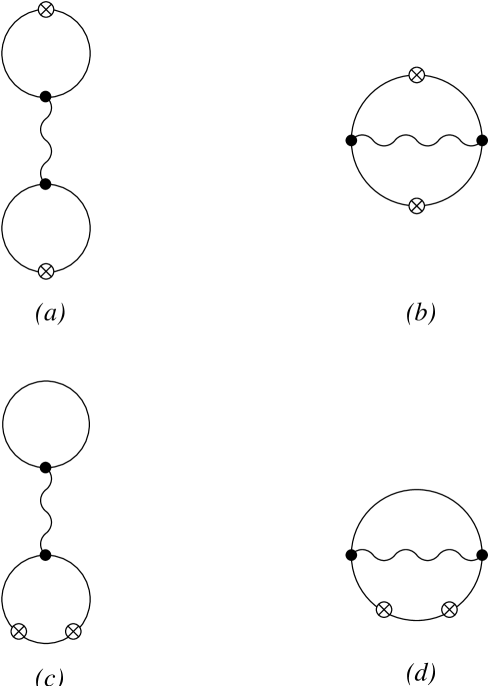
FIG. 2.: Diagrams for the correlator

There is a class of diagrams in Fig. 2 which affect the correlator (7) in a rather trivial way. These are the diagrams (c) and (d), which have both crosses on the same propagator line. Such diagrams give contribution proportional to $\delta^{\alpha\beta}\delta_{{\mathchoice{{\hbox{\boldmath$\displaystyle p$}}}{{\hbox{\boldmath$\textstyle p$}}}{{\hbox{\boldmath$\scriptstyle p$}}}{{\hbox{\boldmath$\scriptscriptstyle p$}}}}{\mathchoice{{\hbox{\boldmath$\displaystyle k$}}}{{\hbox{\boldmath$\textstyle k$}}}{{\hbox{\boldmath$\scriptstyle k$}}}{{\hbox{\boldmath$\scriptscriptstyle k$}}}}}$. These diagrams represent $O(G^{2})$ self-energy type corrections $\delta\omega_{\mathchoice{{\hbox{\boldmath$\displaystyle p$}}}{{\hbox{\boldmath$\textstyle p$}}}{{\hbox{\boldmath$\scriptstyle p$}}}{{\hbox{\boldmath$\scriptscriptstyle p$}}}}$ to $\omega_{\mathchoice{{\hbox{\boldmath$\displaystyle p$}}}{{\hbox{\boldmath$\textstyle p$}}}{{\hbox{\boldmath$\scriptstyle p$}}}{{\hbox{\boldmath$\scriptscriptstyle p$}}}}$ multiplied by a factor $f_{\mathchoice{{\hbox{\boldmath$\displaystyle p$}}}{{\hbox{\boldmath$\textstyle p$}}}{{\hbox{\boldmath$\scriptstyle p$}}}{{\hbox{\boldmath$\scriptscriptstyle p$}}}}{{}^{\prime\prime}}$. Since at zeroth order the correlator is $\delta^{\alpha\beta}\delta_{{\mathchoice{{\hbox{\boldmath$\displaystyle p$}}}{{\hbox{\boldmath$\textstyle p$}}}{{\hbox{\boldmath$\scriptstyle p$}}}{{\hbox{\boldmath$\scriptscriptstyle p$}}}}{\mathchoice{{\hbox{\boldmath$\displaystyle k$}}}{{\hbox{\boldmath$\textstyle k$}}}{{\hbox{\boldmath$\scriptstyle k$}}}{{\hbox{\boldmath$\scriptscriptstyle k$}}}}}f{{}^{\prime}}(\beta\omega_{\mathchoice{{\hbox{\boldmath$\displaystyle p$}}}{{\hbox{\boldmath$\textstyle p$}}}{{\hbox{\boldmath$\scriptstyle p$}}}{{\hbox{\boldmath$\scriptscriptstyle p$}}}})$ (8), one can see that such diagrams are accounted for when we replace $\omega_{\mathchoice{{\hbox{\boldmath$\displaystyle p$}}}{{\hbox{\boldmath$\textstyle p$}}}{{\hbox{\boldmath$\scriptstyle p$}}}{{\hbox{\boldmath$\scriptscriptstyle p$}}}}$ by $\omega_{\mathchoice{{\hbox{\boldmath$\displaystyle p$}}}{{\hbox{\boldmath$\textstyle p$}}}{{\hbox{\boldmath$\scriptstyle p$}}}{{\hbox{\boldmath$\scriptscriptstyle p$}}}}+\delta\omega_{\mathchoice{{\hbox{\boldmath$\displaystyle p$}}}{{\hbox{\boldmath$\textstyle p$}}}{{\hbox{\boldmath$\scriptstyle p$}}}{{\hbox{\boldmath$\scriptscriptstyle p$}}}}$ in $f{{}^{\prime}}(\beta\omega_{\mathchoice{{\hbox{\boldmath$\displaystyle p$}}}{{\hbox{\boldmath$\textstyle p$}}}{{\hbox{\boldmath$\scriptstyle p$}}}{{\hbox{\boldmath$\scriptscriptstyle p$}}}})$.

We shall not study the effects of such self-energy contributions on the correlator or on the single-particle distributions $\langle n_{\mathchoice{{\hbox{\boldmath$\displaystyle p$}}}{{\hbox{\boldmath$\textstyle p$}}}{{\hbox{\boldmath$\scriptstyle p$}}}{{\hbox{\boldmath$\scriptscriptstyle p$}}}}\rangle$. Instead, we assume that these corrections have been already accounted for and we are using corrected $\omega_{\mathchoice{{\hbox{\boldmath$\displaystyle p$}}}{{\hbox{\boldmath$\textstyle p$}}}{{\hbox{\boldmath$\scriptstyle p$}}}{{\hbox{\boldmath$\scriptscriptstyle p$}}}}$. We can view this procedure in the sense of the Wilsonian effective theory approach, and consider the Lagrangian with interaction (11) as the effective Lagrangian. That means no loops (such as self-energy) should be computed with it.From a practical point of view, one can imagine that $\langle n_{\mathchoice{{\hbox{\boldmath$\displaystyle p$}}}{{\hbox{\boldmath$\textstyle p$}}}{{\hbox{\boldmath$\scriptstyle p$}}}{{\hbox{\boldmath$\scriptscriptstyle p$}}}}\rangle$ is measured rather than calculated, and the results are expressed in terms of such measured distribution, instead of $f_{\mathchoice{{\hbox{\boldmath$\displaystyle p$}}}{{\hbox{\boldmath$\textstyle p$}}}{{\hbox{\boldmath$\scriptstyle p$}}}{{\hbox{\boldmath$\scriptscriptstyle p$}}}}$.

With this understanding we can now focus on the most interesting contributions to the correlator, given by the diagrams in Fig. 2(a,b). Differentiating (12) with respect to $\mu^{\alpha}_{\mathchoice{{\hbox{\boldmath$\displaystyle p$}}}{{\hbox{\boldmath$\textstyle p$}}}{{\hbox{\boldmath$\scriptstyle p$}}}{{\hbox{\boldmath$\scriptscriptstyle p$}}}}$ and $\mu^{\beta}_{\mathchoice{{\hbox{\boldmath$\displaystyle k$}}}{{\hbox{\boldmath$\textstyle k$}}}{{\hbox{\boldmath$\scriptstyle k$}}}{{\hbox{\boldmath$\scriptscriptstyle k$}}}}$, and discarding self-energy terms proportional to $\delta_{{\mathchoice{{\hbox{\boldmath$\displaystyle p$}}}{{\hbox{\boldmath$\textstyle p$}}}{{\hbox{\boldmath$\scriptstyle p$}}}{{\hbox{\boldmath$\scriptscriptstyle p$}}}}{\mathchoice{{\hbox{\boldmath$\displaystyle k$}}}{{\hbox{\boldmath$\textstyle k$}}}{{\hbox{\boldmath$\scriptstyle k$}}}{{\hbox{\boldmath$\scriptscriptstyle k$}}}}}$, we find the order $G^{2}$ correction to the correlator:

$$\langle\Delta n^{\alpha}_{\mathchoice{{\hbox{\boldmath$\displaystyle p$}}}{{\hbox{\boldmath$\textstyle p$}}}{{\hbox{\boldmath$\scriptstyle p$}}}{{\hbox{\boldmath$\scriptscriptstyle p$}}}}\,\Delta n^{\beta}_{\mathchoice{{\hbox{\boldmath$\displaystyle k$}}}{{\hbox{\boldmath$\textstyle k$}}}{{\hbox{\boldmath$\scriptstyle k$}}}{{\hbox{\boldmath$\scriptscriptstyle k$}}}}\rangle_{G^{2}}=\beta G^{2}{f_{\mathchoice{{\hbox{\boldmath$\displaystyle p$}}}{{\hbox{\boldmath$\textstyle p$}}}{{\hbox{\boldmath$\scriptstyle p$}}}{{\hbox{\boldmath$\scriptscriptstyle p$}}}}^{\prime}f_{\mathchoice{{\hbox{\boldmath$\displaystyle k$}}}{{\hbox{\boldmath$\textstyle k$}}}{{\hbox{\boldmath$\scriptstyle k$}}}{{\hbox{\boldmath$\scriptscriptstyle k$}}}}^{\prime}\over\omega_{\mathchoice{{\hbox{\boldmath$\displaystyle p$}}}{{\hbox{\boldmath$\textstyle p$}}}{{\hbox{\boldmath$\scriptstyle p$}}}{{\hbox{\boldmath$\scriptscriptstyle p$}}}}\omega_{\mathchoice{{\hbox{\boldmath$\displaystyle k$}}}{{\hbox{\boldmath$\textstyle k$}}}{{\hbox{\boldmath$\scriptstyle k$}}}{{\hbox{\boldmath$\scriptscriptstyle k$}}}}}\left[{\delta^{\alpha\beta}+\gamma^{\alpha\beta}\over\tilde{m}^{2}}+{\gamma^{\alpha\beta}\over\tilde{\omega}_{\mathchoice{{\hbox{\boldmath$\displaystyle q$}}}{{\hbox{\boldmath$\textstyle q$}}}{{\hbox{\boldmath$\scriptstyle q$}}}{{\hbox{\boldmath$\scriptscriptstyle q$}}}}^{2}-(\omega_{\mathchoice{{\hbox{\boldmath$\displaystyle p$}}}{{\hbox{\boldmath$\textstyle p$}}}{{\hbox{\boldmath$\scriptstyle p$}}}{{\hbox{\boldmath$\scriptscriptstyle p$}}}}+\omega_{\mathchoice{{\hbox{\boldmath$\displaystyle k$}}}{{\hbox{\boldmath$\textstyle k$}}}{{\hbox{\boldmath$\scriptstyle k$}}}{{\hbox{\boldmath$\scriptscriptstyle k$}}}})^{2}}+{\delta^{\alpha\beta}\over\tilde{\omega}_{\mathchoice{{\hbox{\boldmath$\displaystyle q$}}}{{\hbox{\boldmath$\textstyle q$}}}{{\hbox{\boldmath$\scriptstyle q$}}}{{\hbox{\boldmath$\scriptscriptstyle q$}}}}^{2}-(\omega_{\mathchoice{{\hbox{\boldmath$\displaystyle p$}}}{{\hbox{\boldmath$\textstyle p$}}}{{\hbox{\boldmath$\scriptstyle p$}}}{{\hbox{\boldmath$\scriptscriptstyle p$}}}}-\omega_{\mathchoice{{\hbox{\boldmath$\displaystyle k$}}}{{\hbox{\boldmath$\textstyle k$}}}{{\hbox{\boldmath$\scriptstyle k$}}}{{\hbox{\boldmath$\scriptscriptstyle k$}}}})^{2}}\right]\,,$$ (18)

where $f_{\mathchoice{{\hbox{\boldmath$\displaystyle p$}}}{{\hbox{\boldmath$\textstyle p$}}}{{\hbox{\boldmath$\scriptstyle p$}}}{{\hbox{\boldmath$\scriptscriptstyle p$}}}}^{\prime}=f_{\mathchoice{{\hbox{\boldmath$\displaystyle p$}}}{{\hbox{\boldmath$\textstyle p$}}}{{\hbox{\boldmath$\scriptstyle p$}}}{{\hbox{\boldmath$\scriptscriptstyle p$}}}}(1+f_{\mathchoice{{\hbox{\boldmath$\displaystyle p$}}}{{\hbox{\boldmath$\textstyle p$}}}{{\hbox{\boldmath$\scriptstyle p$}}}{{\hbox{\boldmath$\scriptscriptstyle p$}}}})$, $\gamma^{+-}=\gamma^{-+}=1$, $\gamma^{++}=\gamma^{--}=0$. The first term in the square brackets is from the diagram in Fig. 2(a), while the second and the third are from Fig. 2(b). A simple way to visualize the $\alpha\beta$ and $\textstyle p$$\textstyle k$ dependence in these three terms is to consider a process of forward scattering $\pi^{\alpha}_{\mathchoice{{\hbox{\boldmath$\displaystyle p$}}}{{\hbox{\boldmath$\textstyle p$}}}{{\hbox{\boldmath$\scriptstyle p$}}}{{\hbox{\boldmath$\scriptscriptstyle p$}}}}\pi^{\beta}_{\mathchoice{{\hbox{\boldmath$\displaystyle k$}}}{{\hbox{\boldmath$\textstyle k$}}}{{\hbox{\boldmath$\scriptstyle k$}}}{{\hbox{\boldmath$\scriptscriptstyle k$}}}}\to\pi^{\alpha}_{\mathchoice{{\hbox{\boldmath$\displaystyle p$}}}{{\hbox{\boldmath$\textstyle p$}}}{{\hbox{\boldmath$\scriptstyle p$}}}{{\hbox{\boldmath$\scriptscriptstyle p$}}}}\pi^{\beta}_{\mathchoice{{\hbox{\boldmath$\displaystyle k$}}}{{\hbox{\boldmath$\textstyle k$}}}{{\hbox{\boldmath$\scriptstyle k$}}}{{\hbox{\boldmath$\scriptscriptstyle k$}}}}$. The three terms arise from contributions with the sigma propagator in $t$, $s$ and $u$ channels respectively, as illustrated in Fig. 3.

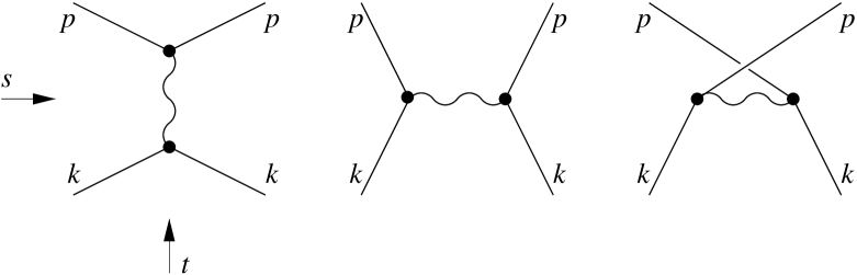
FIG. 3.: A representation of 3 terms in the correlator (18). The resonance is exchanged in $t$, $s$ or $u$ channel.

IV Summary and discussion

In this paper we considered pion gas in thermal equilibrium as an idealization of the final (freezeout) stage of a heavy-ion collision. We considered the effect of pion interaction on the fluctuation correlator (1) or (7) — an important universal quantity characterizing pion fluctuations. Eq. (18) gives the lowest order correction to the correlator (7) due to the interaction mediated by the exchange of $\sigma$-resonance and given by the Lagrangian (11). Our main motivation to consider such an interaction is the search for signatures of the critical point on the QCD phase diagram, the point where the sigma mass vanishes. One can see that the first term in (18), the one due to the sigma exchange in $t$-channel, dominates in the limit $\tilde{m}\to 0$. This term has been already calculated in [7] using a different method. The advantage of the diagrammatic approach of this paper is that it allows one to obtain other terms (due to $s$- and $u$-channel exchange), subleading in the regime $\tilde{m}\to 0$.

Strictly speaking, we have calculated the correction to the correlator only in the leading order of perturbative expansion. Thus, our results are only rigorous in the limit of small coupling constant. Our motivation, however, has been the calculation of a two-particle correlator in hot QCD, which, at temperatures of around 120 MeV, characterizing the freezeout stage of the heavy-ion collisions, is primarily a gas of pions, whose interactions are not controllably small. We observed that, at the leading order, some of the contributions could be naturally absorbed into the self-energy renormalizations. We thus conjectured that if one uses an effective (rather than bare) interaction in (11) and effective self-energies, our leading order calculation could be sufficient in practice.

Below we make several comments and outline some questions and problems, related to the result (18) and its comparison to experimental data. More detailed study of these questions is left to further work.

A Other resonances

The interaction due to the $\sigma$ meson exchange is simpler than interaction due to other resonances, such as $\rho$, but generalization is not difficult. For example, given the effective $\rho^{0}\pi^{+}\pi^{-}$ interaction in the form

$${\cal L}_{\rho\pi\pi}=ig_{\rho\pi\pi}(\rho^{0})^{\mu}\pi^{+}\partial_{\mu}\pi^{-}+{\rm h.c.},$$ (19)

one obtains the contribution of the $\rho$-exchange in the $t$-channel in the form

$$\langle\Delta n^{\alpha}_{\mathchoice{{\hbox{\boldmath$\displaystyle p$}}}{{\hbox{\boldmath$\textstyle p$}}}{{\hbox{\boldmath$\scriptstyle p$}}}{{\hbox{\boldmath$\scriptscriptstyle p$}}}}\,\Delta n^{\beta}_{\mathchoice{{\hbox{\boldmath$\displaystyle k$}}}{{\hbox{\boldmath$\textstyle k$}}}{{\hbox{\boldmath$\scriptstyle k$}}}{{\hbox{\boldmath$\scriptscriptstyle k$}}}}\rangle_{g^{2},t-{\rm channel}}=\beta g_{\rho\pi\pi}^{2}(p\cdot k){f_{\mathchoice{{\hbox{\boldmath$\displaystyle p$}}}{{\hbox{\boldmath$\textstyle p$}}}{{\hbox{\boldmath$\scriptstyle p$}}}{{\hbox{\boldmath$\scriptscriptstyle p$}}}}^{\prime}f_{\mathchoice{{\hbox{\boldmath$\displaystyle k$}}}{{\hbox{\boldmath$\textstyle k$}}}{{\hbox{\boldmath$\scriptstyle k$}}}{{\hbox{\boldmath$\scriptscriptstyle k$}}}}^{\prime}\over\omega_{\mathchoice{{\hbox{\boldmath$\displaystyle p$}}}{{\hbox{\boldmath$\textstyle p$}}}{{\hbox{\boldmath$\scriptstyle p$}}}{{\hbox{\boldmath$\scriptscriptstyle p$}}}}\omega_{\mathchoice{{\hbox{\boldmath$\displaystyle k$}}}{{\hbox{\boldmath$\textstyle k$}}}{{\hbox{\boldmath$\scriptstyle k$}}}{{\hbox{\boldmath$\scriptscriptstyle k$}}}}}{\delta^{\alpha\beta}-\gamma^{\alpha\beta}\over\tilde{m}_{\rho}^{2}}.$$ (20)

Two notable differences from the similar $t$-exchange contribution of $\sigma$ in (18) are worth a notice. Both are due to $\rho$ being a vector particle. First, there is an angular correlation between the pions due to the $(p\cdot k)$ factor. Second, the sign of the correlation now depends on the relative sign of the two pions, due to a minus in $\delta^{\alpha\beta}-\gamma^{\alpha\beta}$.

Similar formulas can be derived for other resonance-mediated interactions of pions. It should be clear that the contribution of the $t$-exchange of $\sigma$-meson is dominant when $m_{\sigma}\to 0$, i.e., near the critical point. It can be further distinguished from other resonance contributions, such as $\rho$, by its charge-independent character ($\delta^{\alpha\beta}+\gamma^{\alpha\beta}=1$ for all $\alpha\beta$). Most importantly, this contribution will show a non-monotonic behavior if the critical point is approached and then passed during the scan of the QCD phase diagram.

B Resonance exchange vs decay

It is important to realize the difference between the result (18) and a more common approach to the correlations due to resonance decays after freezeout [7, 12]. It is easiest to see this difference in the charge dependence of the correlator (18). The term which has the same charge dependence as the contribution of the resonance decays is the one due to $s$-channel exchange: $\sigma$ , or $\rho^{0}$, decays into $\pi^{+}\pi^{-}$, therefore the correlator must be proportional to $\gamma^{\alpha\beta}$. The contribution of $t$ and $u$ channel exchanges is entirely different. In order to compare to experiment, however, one has to take into account the fact that the detected pions consist to a large extent (more than a half) of the products of resonance decays. The contribution of such resonance pions to the correlator should be calculated separately, using the kinematics of the resonance decays. Such a calculation has been done numerically, e.g., in [7] for $p_{T}$ fluctuations, where the effect turned out to be small, except for the contribution of the decay of light $\sigma$ meson near the critical point, and in [12] for charge fluctuations, where the effect is of order 20-30%. The emphasis of this paper is on the correlation induced by virtual resonance exchange among the direct pions.

C $s$-channel pole and resonance width

Generalization to heavier resonances, such as $\rho$, presents another problem. If we consider $\textstyle p$ and $\textstyle k$ such that their invariant mass is equal to $\tilde{m}$, the second term in (18) becomes infinite (the $s$-channel resonance is on mass shell). The perturbative expansion breaks down. However, we know that there is no true pole singularity in this case, since the resonance has a finite lifetime. Thus one would expect that careful treatment of higher order terms should remove this pole divergence and replace it with a smooth Breit-Wigner-type curve. Perhaps, it will also allow to treat resonance exchange and decay within the same formalism (cf. previous subsection).

The $s$-channel divergence does not arise in the application to light $\sigma$ particle near the critical point, since in this case $m_{\sigma}<2m_{\pi}$.

D Longitudinal expansion and rapidity correlator

In this paper we considered an isotropic pion gas (a fireball) at rest. Before one could compare our results to fluctuations observed in heavy-ion collisions it is necessary to take into account the effect of expansion. In this paper we shall only consider longitudinal expansion. It can be taken into account using Bjorken’s boost-invariant hydrodynamic model. In this approximation, one considers a superposition of fireballs placed continuously over large (ideally infinite) rapidity interval. In order to obtain the correlator in this case one needs to take the correlator for a gas at rest $\langle\Delta n^{\alpha}_{\mathchoice{{\hbox{\boldmath$\displaystyle p$}}}{{\hbox{\boldmath$\textstyle p$}}}{{\hbox{\boldmath$\scriptstyle p$}}}{{\hbox{\boldmath$\scriptscriptstyle p$}}}}\,\Delta n^{\beta}_{\mathchoice{{\hbox{\boldmath$\displaystyle k$}}}{{\hbox{\boldmath$\textstyle k$}}}{{\hbox{\boldmath$\scriptstyle k$}}}{{\hbox{\boldmath$\scriptscriptstyle k$}}}}\rangle_{\rm rest}$, boost momenta $\textstyle p$ and $\textstyle k$ with rapidity $y$: ${\langle\Delta n^{\alpha}_{\mathchoice{{\hbox{\boldmath$\displaystyle p$}}}{{\hbox{\boldmath$\textstyle p$}}}{{\hbox{\boldmath$\scriptstyle p$}}}{{\hbox{\boldmath$\scriptscriptstyle p$}}}\oplus y}\,\Delta n^{\beta}_{\mathchoice{{\hbox{\boldmath$\displaystyle k$}}}{{\hbox{\boldmath$\textstyle k$}}}{{\hbox{\boldmath$\scriptstyle k$}}}{{\hbox{\boldmath$\scriptscriptstyle k$}}}\oplus y}\rangle}_{\rm rest}$ and integrate over $y$:

$$\langle\Delta n^{\alpha}_{\mathchoice{{\hbox{\boldmath$\displaystyle p$}}}{{\hbox{\boldmath$\textstyle p$}}}{{\hbox{\boldmath$\scriptstyle p$}}}{{\hbox{\boldmath$\scriptscriptstyle p$}}}}\,\Delta n^{\beta}_{\mathchoice{{\hbox{\boldmath$\displaystyle k$}}}{{\hbox{\boldmath$\textstyle k$}}}{{\hbox{\boldmath$\scriptstyle k$}}}{{\hbox{\boldmath$\scriptscriptstyle k$}}}}\rangle_{\rm long.exp.}\equiv\int_{-\infty}^{+\infty}dy\,\omega_{{\mathchoice{{\hbox{\boldmath$\displaystyle p$}}}{{\hbox{\boldmath$\textstyle p$}}}{{\hbox{\boldmath$\scriptstyle p$}}}{{\hbox{\boldmath$\scriptscriptstyle p$}}}}\oplus y}\,\omega_{{\mathchoice{{\hbox{\boldmath$\displaystyle k$}}}{{\hbox{\boldmath$\textstyle k$}}}{{\hbox{\boldmath$\scriptstyle k$}}}{{\hbox{\boldmath$\scriptscriptstyle k$}}}}\oplus y}\,{\langle\Delta n^{\alpha}_{\mathchoice{{\hbox{\boldmath$\displaystyle p$}}}{{\hbox{\boldmath$\textstyle p$}}}{{\hbox{\boldmath$\scriptstyle p$}}}{{\hbox{\boldmath$\scriptscriptstyle p$}}}\oplus y}\,\Delta n^{\beta}_{\mathchoice{{\hbox{\boldmath$\displaystyle k$}}}{{\hbox{\boldmath$\textstyle k$}}}{{\hbox{\boldmath$\scriptstyle k$}}}{{\hbox{\boldmath$\scriptscriptstyle k$}}}\oplus y}\rangle}_{\rm rest}.$$ (21)

The factors $\omega_{\mathchoice{{\hbox{\boldmath$\displaystyle p$}}}{{\hbox{\boldmath$\textstyle p$}}}{{\hbox{\boldmath$\scriptstyle p$}}}{{\hbox{\boldmath$\scriptscriptstyle p$}}}}$, $\omega_{\mathchoice{{\hbox{\boldmath$\displaystyle k$}}}{{\hbox{\boldmath$\textstyle k$}}}{{\hbox{\boldmath$\scriptstyle k$}}}{{\hbox{\boldmath$\scriptscriptstyle k$}}}}$ appear because of the non-uniform density of modes in rapidity space, i.e., $d^{3}{\mathchoice{{\hbox{\boldmath$\displaystyle p$}}}{{\hbox{\boldmath$\textstyle p$}}}{{\hbox{\boldmath$\scriptstyle p$}}}{{\hbox{\boldmath$\scriptscriptstyle p$}}}}=\omega_{\mathchoice{{\hbox{\boldmath$\displaystyle p$}}}{{\hbox{\boldmath$\textstyle p$}}}{{\hbox{\boldmath$\scriptstyle p$}}}{{\hbox{\boldmath$\scriptscriptstyle p$}}}}\,d^{2}{\mathchoice{{\hbox{\boldmath$\displaystyle p$}}}{{\hbox{\boldmath$\textstyle p$}}}{{\hbox{\boldmath$\scriptstyle p$}}}{{\hbox{\boldmath$\scriptscriptstyle p$}}}}_{T}\,dy_{\mathchoice{{\hbox{\boldmath$\displaystyle p$}}}{{\hbox{\boldmath$\textstyle p$}}}{{\hbox{\boldmath$\scriptstyle p$}}}{{\hbox{\boldmath$\scriptscriptstyle p$}}}}$ ($y_{\mathchoice{{\hbox{\boldmath$\displaystyle p$}}}{{\hbox{\boldmath$\textstyle p$}}}{{\hbox{\boldmath$\scriptstyle p$}}}{{\hbox{\boldmath$\scriptscriptstyle p$}}}}={\rm atanh}(p_{z}/\omega_{\mathchoice{{\hbox{\boldmath$\displaystyle p$}}}{{\hbox{\boldmath$\textstyle p$}}}{{\hbox{\boldmath$\scriptstyle p$}}}{{\hbox{\boldmath$\scriptscriptstyle p$}}}})$, ${\mathchoice{{\hbox{\boldmath$\displaystyle p$}}}{{\hbox{\boldmath$\textstyle p$}}}{{\hbox{\boldmath$\scriptstyle p$}}}{{\hbox{\boldmath$\scriptscriptstyle p$}}}}_{T}=(p_{x},p_{y})$).

As a practical example, one can use formula (21) to determine the form of rapidity correlations. For this purpose one needs to fix rapidities $y_{\mathchoice{{\hbox{\boldmath$\displaystyle p$}}}{{\hbox{\boldmath$\textstyle p$}}}{{\hbox{\boldmath$\scriptstyle p$}}}{{\hbox{\boldmath$\scriptscriptstyle p$}}}}$ and $y_{\mathchoice{{\hbox{\boldmath$\displaystyle k$}}}{{\hbox{\boldmath$\textstyle k$}}}{{\hbox{\boldmath$\scriptstyle k$}}}{{\hbox{\boldmath$\scriptscriptstyle k$}}}}$, and integrate over transverse components ${\mathchoice{{\hbox{\boldmath$\displaystyle p$}}}{{\hbox{\boldmath$\textstyle p$}}}{{\hbox{\boldmath$\scriptstyle p$}}}{{\hbox{\boldmath$\scriptscriptstyle p$}}}}_{T}$ and ${\mathchoice{{\hbox{\boldmath$\displaystyle k$}}}{{\hbox{\boldmath$\textstyle k$}}}{{\hbox{\boldmath$\scriptstyle k$}}}{{\hbox{\boldmath$\scriptscriptstyle k$}}}}_{T}$:

$$C^{\alpha\beta}(y_{\mathchoice{{\hbox{\boldmath$\displaystyle p$}}}{{\hbox{\boldmath$\textstyle p$}}}{{\hbox{\boldmath$\scriptstyle p$}}}{{\hbox{\boldmath$\scriptscriptstyle p$}}}},y_{\mathchoice{{\hbox{\boldmath$\displaystyle k$}}}{{\hbox{\boldmath$\textstyle k$}}}{{\hbox{\boldmath$\scriptstyle k$}}}{{\hbox{\boldmath$\scriptscriptstyle k$}}}})={dN/dy\over\int_{\mathchoice{{\hbox{\boldmath$\displaystyle p$}}}{{\hbox{\boldmath$\textstyle p$}}}{{\hbox{\boldmath$\scriptstyle p$}}}{{\hbox{\boldmath$\scriptscriptstyle p$}}}}f_{\mathchoice{{\hbox{\boldmath$\displaystyle p$}}}{{\hbox{\boldmath$\textstyle p$}}}{{\hbox{\boldmath$\scriptstyle p$}}}{{\hbox{\boldmath$\scriptscriptstyle p$}}}}}\int_{{\mathchoice{{\hbox{\boldmath$\displaystyle p$}}}{{\hbox{\boldmath$\textstyle p$}}}{{\hbox{\boldmath$\scriptstyle p$}}}{{\hbox{\boldmath$\scriptscriptstyle p$}}}}_{T}}\int_{{\mathchoice{{\hbox{\boldmath$\displaystyle k$}}}{{\hbox{\boldmath$\textstyle k$}}}{{\hbox{\boldmath$\scriptstyle k$}}}{{\hbox{\boldmath$\scriptscriptstyle k$}}}}_{T}}\langle\Delta n^{\alpha}_{\mathchoice{{\hbox{\boldmath$\displaystyle p$}}}{{\hbox{\boldmath$\textstyle p$}}}{{\hbox{\boldmath$\scriptstyle p$}}}{{\hbox{\boldmath$\scriptscriptstyle p$}}}}\,\Delta n^{\beta}_{\mathchoice{{\hbox{\boldmath$\displaystyle k$}}}{{\hbox{\boldmath$\textstyle k$}}}{{\hbox{\boldmath$\scriptstyle k$}}}{{\hbox{\boldmath$\scriptscriptstyle k$}}}}\rangle_{\rm long.exp.},$$ (22)

where $\int_{{\mathchoice{{\hbox{\boldmath$\displaystyle p$}}}{{\hbox{\boldmath$\textstyle p$}}}{{\hbox{\boldmath$\scriptstyle p$}}}{{\hbox{\boldmath$\scriptscriptstyle p$}}}}_{T}}\equiv\int d^{2}{\mathchoice{{\hbox{\boldmath$\displaystyle p$}}}{{\hbox{\boldmath$\textstyle p$}}}{{\hbox{\boldmath$\scriptstyle p$}}}{{\hbox{\boldmath$\scriptscriptstyle p$}}}}_{T}/(2\pi)^{3}$. The normalization factor, $(dN/dy)/(\int_{\mathchoice{{\hbox{\boldmath$\displaystyle p$}}}{{\hbox{\boldmath$\textstyle p$}}}{{\hbox{\boldmath$\scriptstyle p$}}}{{\hbox{\boldmath$\scriptscriptstyle p$}}}}f_{\mathchoice{{\hbox{\boldmath$\displaystyle p$}}}{{\hbox{\boldmath$\textstyle p$}}}{{\hbox{\boldmath$\scriptstyle p$}}}{{\hbox{\boldmath$\scriptscriptstyle p$}}}})$, is such that $C(y_{\mathchoice{{\hbox{\boldmath$\displaystyle p$}}}{{\hbox{\boldmath$\textstyle p$}}}{{\hbox{\boldmath$\scriptstyle p$}}}{{\hbox{\boldmath$\scriptscriptstyle p$}}}},y_{\mathchoice{{\hbox{\boldmath$\displaystyle k$}}}{{\hbox{\boldmath$\textstyle k$}}}{{\hbox{\boldmath$\scriptstyle k$}}}{{\hbox{\boldmath$\scriptscriptstyle k$}}}})=\rho_{2}(y_{\mathchoice{{\hbox{\boldmath$\displaystyle p$}}}{{\hbox{\boldmath$\textstyle p$}}}{{\hbox{\boldmath$\scriptstyle p$}}}{{\hbox{\boldmath$\scriptscriptstyle p$}}}},y_{\mathchoice{{\hbox{\boldmath$\displaystyle k$}}}{{\hbox{\boldmath$\textstyle k$}}}{{\hbox{\boldmath$\scriptstyle k$}}}{{\hbox{\boldmath$\scriptscriptstyle k$}}}})-\rho(y_{\mathchoice{{\hbox{\boldmath$\displaystyle p$}}}{{\hbox{\boldmath$\textstyle p$}}}{{\hbox{\boldmath$\scriptstyle p$}}}{{\hbox{\boldmath$\scriptscriptstyle p$}}}})\rho(y_{\mathchoice{{\hbox{\boldmath$\displaystyle k$}}}{{\hbox{\boldmath$\textstyle k$}}}{{\hbox{\boldmath$\scriptstyle k$}}}{{\hbox{\boldmath$\scriptscriptstyle k$}}}})$, where $\rho=dN/dy$ and $\rho_{2}$ is the density of pairs per unit rapidity squared.

Using expression (21) in (22) one finds, of course, that correlator $C(y_{\mathchoice{{\hbox{\boldmath$\displaystyle p$}}}{{\hbox{\boldmath$\textstyle p$}}}{{\hbox{\boldmath$\scriptstyle p$}}}{{\hbox{\boldmath$\scriptscriptstyle p$}}}},y_{\mathchoice{{\hbox{\boldmath$\displaystyle k$}}}{{\hbox{\boldmath$\textstyle k$}}}{{\hbox{\boldmath$\scriptstyle k$}}}{{\hbox{\boldmath$\scriptscriptstyle k$}}}})$ is a function of $y_{\mathchoice{{\hbox{\boldmath$\displaystyle p$}}}{{\hbox{\boldmath$\textstyle p$}}}{{\hbox{\boldmath$\scriptstyle p$}}}{{\hbox{\boldmath$\scriptscriptstyle p$}}}}-y_{\mathchoice{{\hbox{\boldmath$\displaystyle k$}}}{{\hbox{\boldmath$\textstyle k$}}}{{\hbox{\boldmath$\scriptstyle k$}}}{{\hbox{\boldmath$\scriptscriptstyle k$}}}}$ only. The dependence on $y_{\mathchoice{{\hbox{\boldmath$\displaystyle p$}}}{{\hbox{\boldmath$\textstyle p$}}}{{\hbox{\boldmath$\scriptstyle p$}}}{{\hbox{\boldmath$\scriptscriptstyle p$}}}}-y_{\mathchoice{{\hbox{\boldmath$\displaystyle k$}}}{{\hbox{\boldmath$\textstyle k$}}}{{\hbox{\boldmath$\scriptstyle k$}}}{{\hbox{\boldmath$\scriptscriptstyle k$}}}}$ can be found substituting (18) for $\langle\Delta n^{\alpha}_{\mathchoice{{\hbox{\boldmath$\displaystyle p$}}}{{\hbox{\boldmath$\textstyle p$}}}{{\hbox{\boldmath$\scriptstyle p$}}}{{\hbox{\boldmath$\scriptscriptstyle p$}}}}\,\Delta n^{\beta}_{\mathchoice{{\hbox{\boldmath$\displaystyle k$}}}{{\hbox{\boldmath$\textstyle k$}}}{{\hbox{\boldmath$\scriptstyle k$}}}{{\hbox{\boldmath$\scriptscriptstyle k$}}}}\rangle_{\rm rest}$ in (21). The detailed form of the correlator depends on the parameters $G$, $\tilde{m}$, $\beta=1/T$. A rather robust feature of $C(y_{\mathchoice{{\hbox{\boldmath$\displaystyle p$}}}{{\hbox{\boldmath$\textstyle p$}}}{{\hbox{\boldmath$\scriptstyle p$}}}{{\hbox{\boldmath$\scriptscriptstyle p$}}}}-y_{\mathchoice{{\hbox{\boldmath$\displaystyle k$}}}{{\hbox{\boldmath$\textstyle k$}}}{{\hbox{\boldmath$\scriptstyle k$}}}{{\hbox{\boldmath$\scriptscriptstyle k$}}}})$, however, is that it vanishes exponentially with increasing $|y_{\mathchoice{{\hbox{\boldmath$\displaystyle p$}}}{{\hbox{\boldmath$\textstyle p$}}}{{\hbox{\boldmath$\scriptstyle p$}}}{{\hbox{\boldmath$\scriptscriptstyle p$}}}}-y_{\mathchoice{{\hbox{\boldmath$\displaystyle k$}}}{{\hbox{\boldmath$\textstyle k$}}}{{\hbox{\boldmath$\scriptstyle k$}}}{{\hbox{\boldmath$\scriptscriptstyle k$}}}}|$ on the scale of 1-2 units. This is because of the fast exponential falloff of the occupation number factors $f_{\mathchoice{{\hbox{\boldmath$\displaystyle p$}}}{{\hbox{\boldmath$\textstyle p$}}}{{\hbox{\boldmath$\scriptstyle p$}}}{{\hbox{\boldmath$\scriptscriptstyle p$}}}}f_{\mathchoice{{\hbox{\boldmath$\displaystyle k$}}}{{\hbox{\boldmath$\textstyle k$}}}{{\hbox{\boldmath$\scriptstyle k$}}}{{\hbox{\boldmath$\scriptscriptstyle k$}}}}$ in (18) when either $\textstyle p$ or $\textstyle k$ becomes large compared to $T$. As an example, the contribution to the rapidity correlator from the $t$-channel exchange term only, i.e., first term in (18), is shown in Fig. 4.

FIG. 4.: A typical contribution to rapidity correlator. $y\equiv|y_{\mathchoice{{\hbox{\boldmath$\displaystyle p$}}}{{\hbox{\boldmath$\textstyle p$}}}{{\hbox{\boldmath$\scriptstyle p$}}}{{\hbox{\boldmath$\scriptscriptstyle p$}}}}-y_{\mathchoice{{\hbox{\boldmath$\displaystyle k$}}}{{\hbox{\boldmath$\textstyle k$}}}{{\hbox{\boldmath$\scriptstyle k$}}}{{\hbox{\boldmath$\scriptscriptstyle k$}}}}|$. In this example, $T=120$ MeV, $G/\tilde{m}=4.5$ (see [7, 8] for motivation). Plotted is the correlator $C$ in (22) divided by $dN/dy$.

Another interesting consequence of (18) is a specific dependence on multiplicity $dN/dy$. For example, the centrality dependence of the freezeout parameters is known to be rather weak. Neglecting it, we could predict, using (18), that the centrality dependence comes only from the factor $dN/dy$, and is, therefore, linear.

REFERENCES

- [1] H. Appelshauser et al. [NA49 Collaboration], Phys. Lett. B 459, 679 (1999); J. G. Reid [NA49 Collaboration], Nucl. Phys. A 661, 407 (1999); S. V. Afanasev et al. [NA49 Collaboration], Phys. Rev. Lett. 86, 1965 (2001); J. Bachler et al. [NA49 Collaboration], Nucl. Phys. Proc. Suppl. 92, 7 (2001).
- [2] J. Reid [STAR Collaboration], in proceedings of 15th International Conference on Ultrarelativistic Nucleus-Nucleus Collisions (QM2001), Stony Brook, New York, 15-20 Jan 2001; S. A. Voloshin [STAR Collaboration], arXiv:nucl-ex/0109006.
- [3] V. Friese et al. [NA49 Collab], in proceedings of International Symposium on Multiparticle Dynamics, Datong, China, Sept. 1-7,2001, to be published by World Scientific.
- [4] L. Stodolsky, Phys. Rev. Lett. 75, 1044 (1995); E. V. Shuryak, Phys. Lett. B 423, 9 (1998).
- [5] M. Gazdzicki and S. Mrowczynski, Z. Phys. C 54, 127 (1992); M. Gazdzicki, A. Leonidov and G. Roland, Eur. Phys. J. C 6, 365 (1999).
- [6] M. Stephanov, K. Rajagopal and E. V. Shuryak, Phys. Rev. Lett. 81, 4816 (1998).
- [7] M. Stephanov, K. Rajagopal and E. V. Shuryak, Phys. Rev. D 60, 114028 (1999).
- [8] B. Berdnikov and K. Rajagopal, Phys. Rev. D 61, 105017 (2000).
- [9] A. Bialas and V. Koch, Phys. Lett. B 456, 1 (1999); M. Belkacem, Z. Aouissat, M. Bleicher, H. Stocker and W. Greiner, arXiv:nucl-th/9903017.
- [10] S. A. Voloshin, V. Koch and H. G. Ritter, arXiv:nucl-th/9903060.
- [11] G. Baym and H. Heiselberg, Phys. Lett. B 469, 7 (1999). G. V. Danilov and E. V. Shuryak, arXiv:nucl-th/9908027.
- [12] S. Jeon and V. Koch, Phys. Rev. Lett. 83, 5435 (1999).
- [13] M. Asakawa, U. W. Heinz and B. Muller, Phys. Rev. Lett. 85, 2072 (2000); S. Jeon and V. Koch, Phys. Rev. Lett. 85, 2076 (2000); M. Bleicher, S. Jeon and V. Koch, Phys. Rev. C 62, 061902 (2000).
- [14] S. A. Bass, P. Danielewicz and S. Pratt, Phys. Rev. Lett. 85, 2689 (2000).
- [15] H. Heiselberg and A. D. Jackson, Phys. Rev. C 63, 064904 (2001).
- [16] M. Gazdzicki and S. Mrowczynski, arXiv:nucl-th/0012094.
- [17] E. V. Shuryak and M. A. Stephanov, Phys. Rev. C 63, 064903 (2001).
- [18] R. C. Hwa and C. B. Yang, arXiv:hep-ph/0104216.
- [19] D. Bower and S. Gavin, Phys. Rev. C 64, 051902 (2001).
- [20] S. Mrowczynski, Phys. Lett. B 465, 8 (1999); Acta Phys. Polon. B 31, 2065 (2000).
- [21] R. Korus, S. Mrowczynski, M. Rybczynski and Z. Wlodarczyk, arXiv:nucl-th/0106041.
- [22] P. Braun-Munzinger, J. Stachel, J. P. Wessels and N. Xu, Phys. Lett. B 344, 43 (1995); Phys. Lett. B 365, 1 (1996); P. Braun-Munzinger, I. Heppe and J. Stachel, Phys. Lett. B 465, 15 (1999).
- [23] K. Rajagopal, Nucl. Phys. A 680, 211 (2000).
- [24] L. D. Landau and E. M. Lifshitz, Statistical Physics, Part 1 (Pergamon, 1980).
- [25] U. W. Heinz and B. V. Jacak, Ann. Rev. Nucl. Part. Sci. 49, 529 (1999).
- [26] A.A. Abrikosov, L.P.Gorkov and I.E. Dzyaloshinski, Methods of quantum field theory in statistical physics, (Dover, New York, 1975).
- [27] H. A. Weldon, Phys. Rev. D 28, 2007 (1983).
- [28] R. D. Pisarski, Nucl. Phys. B 309, 476 (1988).
- [29] J. D. Bjorken, Phys. Rev. D 27, 140 (1983).