Femto-Photography of Protons to Nuclei with Deeply Virtual Compton Scattering

Abstract

Developments in deeply virtual Compton scattering allow the direct measurements of scattering amplitudes for exchange of a highly virtual photon with fine spatial resolution. Real-space images of the target can be obtained from this information. Spatial resolution is determined by the momentum transfer rather than the wavelength of the detected photon. Quantum photographs of the proton, nuclei, and other elementary particles with resolution on the scale of a fraction of a femtometer is feasible with existing experimental technology.

More than 40 years ago, elastic scattering of relativistic electrons from protons by Hofstadter[1] et al probed the dimensions of protons and nuclei. On general principles the scattering is governed by “form factors”, which parameterize the difference between point-like scattering and the observations. In static non-relativistic approximations of the era, the form factors were interpreted as “…determining the distribution of charge and magnetic moment in the nuclei of atoms and of the nucleons themselves”[2], with the experiments receiving the Nobel Prize in 1961. The charge radius was found to be about 0.7 femtometer. The neutron’s form factor was later interpreted in terms of a positively charged core surrounded by a negatively charged outer shell. In retrospect, these classic interpretations are open to doubt. Neither the impulse approximation nor the interpretation as charge density applies so simply to hadronic physics in the regime of the experiments. Point-like structure now attributed to quarks has been deduced indirectly, in conjunction with the development of Quantum Chromodynamics and deeply inelastic scattering experiments (DIS). The structure of hadrons as complex aggregates of quarks remains rather mysterious.

Deeply virtual Compton scattering (DVCS)[3] combines features of the inelastic processes with those of an elastic process. A relativistic charged lepton (electron, positron, or possibly a muon) is scattered from a target nucleon or nucleus. A real photon of 4-momentum $q_{\mu}^{\prime}=(q_{0}^{\prime},\vec{q}^{\prime})$ is also observed in the final state. With $e(k),\,e^{\prime}(k^{\prime})$ denoting the initial and final electrons of momenta $k,\,k^{\prime}$ respectively, and $P,\,P^{\prime}$ denoting the momentum of the target, the process is

$$e(k)+P\rightarrow e^{\prime}(k^{\prime})+P^{\prime}+\gamma(q^{\prime}).$$

The net momentum transfer $\Delta$ to the target is obtained by momentum conservation, $\Delta^{\mu}=k^{\mu}-k^{`\,\mu}-q^{`\,\mu}$. The real photon may be emitted by the lepton beam, in which case a virtual photon of momentum $Q_{BH}^{\mu}=\Delta^{\mu}$ strikes the target. Otherwise the target emits the real photon and a virtual photon of $Q_{VCS}^{\mu}=P^{\prime\mu}-P^{\mu}+q^{`\,\mu}$ strikes the target. It is straightforward to select events where all components of $\Delta^{\mu}$ are small compared to $\sqrt{Q^{2}}$, with $Q^{2}=-Q_{VCS}^{\mu}Q_{VCS,\,\mu}>GeV^{2}$. These conditions have recently been realized in experiments at HERMES[4] at DESY and CEBAF[4] at JLab.

The physical interpretation is that the target is resolved by the virtual photon on a spatial scale small compared to the target size. A photon of high virtuality $Q^{2}$ selects a short-distance region of the target: the spatial resolution is of order $\Delta b_{T}\sim\hbar/\sqrt{Q^{2}}$. In contrast, high energy real photons ($(q^{\prime})^{2}=0$) are not well localized, and do not interact in a consistent point-like manner described by simple impulse approximations. Perturbative QCD (pQCD) can be applied to DVCS at large $Q^{2}$ , exploiting the short-distance resolution of the virtual photon, despite the presence of a real photon in the reaction. [3, 5]

Meanwhile the net momentum transfer $\Delta^{\mu}$ is independent, and Fourier-conjugate to the spatial location where the virtual photon scattering event occurs. Let us review this[6]. We use a conventional Lorentz frame with coordinates (+, T, -) where $P^{2}=2P^{+}P^{-}-\vec{P}_{T}^{2}$:

$$P^{\mu}=(P^{+},\,-\vec{\Delta}_{T}/2,\,\frac{m^{2}+\Delta_{T}^{2}/4}{2P^{+}});$$

$$P^{\prime\mu}=(P^{+}+\Delta^{+},\,+\vec{\Delta}_{T}/2,\,\frac{m^{2}+\Delta_{T}^{2}/4}{2P^{+}+2\Delta^{+}});$$

$$q^{\mu}=(Q_{VCS},\,0,\,Q_{VCS})/\sqrt{2};$$

$$q^{\prime\mu}=(Q_{VCS}/\sqrt{2}-\Delta^{+},-\vec{\Delta}_{T},\frac{\Delta_{T}^{2}}{2(Q_{VCS}/\sqrt{2}-\Delta^{+})}).$$

We also write $\Delta^{\mu}=\zeta P^{\mu}+\Delta_{T}^{\mu},$ $\Delta^{\mu}\Delta_{\mu}=t<0$. Here $m$ is the target mass and $\zeta/2$ is denoted the “ skewness”.

The impulse approximation applies in the infinite momentum frames $P^{+}\rightarrow\infty$, $x_{Bj}=Q_{VCS}^{2}/2P\cdot q$ fixed and not too small. The handbag diagram represents dominance by the quark-proton scattering amplitude $\Phi$ upon which both diagonal and off-diagonal (generalized) parton distributions are based. Our notation is

$$\Phi^{\rho\sigma}(\kappa,\kappa^{\prime})_{P,P^{\prime}}=$$

$$\int dx_{1}dx_{2}\,e^{i\kappa\cdot x_{1}-i\kappa^{\prime}\cdot x_{2}}<P^{\prime},s^{\prime}|T\psi_{\rho}(x_{2})\bar{\psi}_{\sigma}(x_{1})|P,s>.$$ (1)

This object is relevant to the analysis in the region[7] $-t_{min}<-t<-t_{max}\sim GeV^{2}$. By momentum conservation $\kappa^{\prime}-\kappa=P^{\prime}-P=\Delta$. The quark fields are evaluated at spatial coordinates $x_{1},\,x_{2}$ and have Dirac indices $\rho,\sigma$. We may rewrite

$$e^{i\kappa\cdot x_{1}-i\kappa^{\prime}\cdot x_{2}}=e^{i\frac{\kappa+\kappa^{\prime}}{2}\cdot(x_{1}-x_{2})-i\Delta\cdot\frac{x_{1}+x_{2}}{2}}.$$

When diagonalized, and combined with unitarity, imaginary parts of transition amplitude such as $\Phi$ can also be viewed as parton probabilities for certain reactions. Our emphasis retains the amplitude interpretation.

By superposition the target state is represented as

$$|P,s>=\int dY\;exp(-iP\cdot Y)|Y,s>,$$

where $Y$ is a center of momentum ($CM$) coordinate. With a similar step for $|P^{\prime}>$, we have matrix elements depending on $e^{-iP\cdot Y+iP^{\prime}\cdot Y^{\prime}}=e^{-i\frac{P+P^{\prime}}{2}\cdot(Y-Y^{\prime})+i\Delta\cdot\frac{Y+Y^{\prime}}{2}}.$ These steps isolate all dependence on the variable $\Delta$ in

$$\Phi^{\rho\sigma}(\kappa,\kappa^{\prime})_{P,P^{\prime}}=$$

$$\int dYdY^{\prime}\,dx_{1}dx_{2}\bar{\Phi}e^{-i\frac{P+P^{\prime}}{2}\cdot(Y-Y^{\prime})+i\frac{\kappa+\kappa^{\prime}}{2}\cdot(x_{1}-x_{2})}e^{-i\Delta\cdot(-\bar{Y}+\bar{b})},$$

where $\bar{\Phi}_{\rho\sigma}=<Y^{\prime},s^{\prime}|\psi_{\rho}(z^{\prime})\bar{\psi}_{\sigma}(z)|Y,s>$ , $\bar{Y}=(Y+Y^{\prime})/2,$ and

$$\bar{b}=(x_{2}+x_{1})/2.$$

The new feature of $GPD$ is given by the $\Delta$ dependence[8, 9, 6]. From the Fourier expansions, the $\Delta$ dependence is interpreted as a measurement of the conjugate variable $\bar{b}-\bar{Y}$. This space-time variable is the average spatial offset of the struck quarks relative to the $CM$ location of the hadrons, as resolved on the hard scale $1/\sqrt{Q^{2}}$. The concept of “average spatial offset” cannot be formulated in the forward limit $\Delta\rightarrow 0$ probed in inclusive experiments. Thus the object of our study, the spatial location of the struck quarks inside the proton, cannot in principle be addressed by the traditional inelastic observables. Yet the spatial location is gauge-invariant, local, and underlies all the sophisticated technical studies of the applicability of QCD.[10, 3]. The dependence on where the hadron $CM$ is located, $\bar{Y}$, appears as a trivial overall phase in the amplitudes; we may therefore set $\bar{Y}\rightarrow 0$. Then $\bar{b}$ is the average spatial location of the quark correlations relative to that origin. This clearly represents a new variable compared to the separation between the quark fields in correlations familiar to workers involved in DIS.

The $\Delta$ dependence, in turn, can be converted back into the spatial location of the struck quarks by doing the inverse Fourier transform. Elementary consideration reveals that this amounts to introduction of a “focusing lens” of mathematical sort. Indeed, the action of an ordinary (perfect, thin) lens in focusing light consists of Fourier transforming the ray representation (momentum) into the spatial representation. The modulus of the spatial amplitude-squared is the intensity in the image plane. Thus, while it is impossible to focus gamma-rays of GeV energies well with any material instruments, the focusing can be obtained mathematically, if only the amplitudes of the gamma rays emissions are known.

We turn to the underlying reasons that the gamma-ray amplitudes can be measured. The cross section $d\sigma\sim\sum_{if}\,M_{if}M_{if}^{*}$ where $M_{if}$ is the transition matrix element, and $i,\,f$ are indices, such as spins, summed over experimentally, and described in detail below. DVCS has $M=M_{BH}+M_{e+target}$ where $M_{BH}$ is the Bethe-Heitler amplitude for the emission from the electrons, and $M_{e+target}$ is the emission from the target struck by the electron or positron. The interference term $d\sigma_{int}=2Re\sum_{if}\ [M_{BH}^{*}(\Delta)M_{e+target}(\Delta)\ ]$ can be obtained by subtraction since $|M_{BH}|^{2}$ is known. Symbol $M_{e+target}$ is already contracted with the amplitude $L^{\nu}$ for $\gamma^{*}$ emission from the lepton beam: with indices explicit, $M_{e+target}^{\mu}=M_{target;\,s\ ,s^{\prime};\,\mu\nu}L^{\nu}$ to emit final state polarization $\mu$. Symbol $M_{BH}$ includes the lepton amplitudes contracted with $<p^{\prime},\,s^{\prime}|J_{em}^{\rho}|p,\,s>$, and depends on $s,\,s^{\prime}$. The experimentally measured form factors, not an impulse approximation, are used to predict $M_{BH}$. Measuring the interference term is practical due to copious electron radiation, $|M_{BH}|>>|M_{target}|$, which is the generic situation at moderate energies[4].

The interference term can be written

$$\sum_{ss^{\prime}\,\mu\nu}L^{\nu}M_{BH;\,ss^{\prime}}^{\mu*}(\Delta)M_{target;\,s\ ,s^{\prime};\,\mu\nu}(\Delta)+c.\,c.;$$

$$=tr\ [\,L\,M_{BH}^{\dagger}(\Delta)\,M_{target}(\Delta)\,\ ]+c.\,c.$$ (2)

Here $c.\,c.$ indicates the complex conjugate and $tr$ indicates the trace over the joint indices of proton spins $s,\,s^{\prime}$ and photon polarizations $\mu,\,\nu$. The matrix $\Lambda_{s\,s^{\prime}}^{\mu\nu}=L^{\nu}M_{BH;\,ss^{\prime}}^{\mu*}$ can be expanded in an orthonormal joint basis $m^{j}$ on the space of all matrices, with $tr((m^{j})^{\dagger}m^{k})=\delta^{jk}$. Choose the first basis element $m_{ss^{\prime};\,\mu\nu}^{1}(\Delta)=\Lambda_{s\,s^{\prime}}^{\mu\nu}/\sqrt{tr(\Lambda^{\dagger}\Lambda)}$ “parallel” to the Bethe-Heitler amplitude itself. Then $M_{BH}(\Delta)=\mu^{1}(\Delta)m^{1}(\Delta)$ with $\mu^{1}$ a scalar coefficient. All of the factors being known, the trace projects out a unique amplitude $M_{T;\,s\,s^{\prime}\,}^{\mu\nu}(\Delta)=A(\Delta)m_{ss^{\prime};\,\mu\nu}^{1}(\Delta)$, where $A(\Delta)$ is a Lorentz scalar. We suppressed other dependences to highlight how the irrelevant $\Delta$-dependence in the scalar coefficient $\mu_{1}(\Delta)$ has been removed. Up to normalization conventions, $M_{T;\,s\,s^{\prime}\,}^{\mu\nu}(\Delta)$ equals the Fourier transform of $<p^{\prime},\,s^{\prime}|\,T\ [\,J_{em}^{\mu}(x)J_{em}^{\nu}(x^{\prime})\,\ ]\,|p,\,s>$. The observable amplitude is the textbook amplitude; the GPD and handbag kernels are constructs justifying its interpretation. An unpolarized experiment may extract only a real or imaginary part of the amplitude, as reviewed below. A spin-dependent amplitude determination is made even from unpolarized targets.

This remarkable feature has a physical explanation. In the emission of $\gamma(q^{\prime})$, both the electron beam and the target contribute amplitudes, which quantum-mechanically interfere. The virtual photon strikes the target hard, causing acceleration of the internal constituents and emission of a real photon from near the struck point, in the handbag model. Simultaneously the electron beam acts as a known coherent reference sources, and emits a photon with known quantum numbers. Amplitudes orthogonal to the reference source may be emitted by the target, but they cannot be observed by interference: the experimental conditions of the lepton beam and polarization sums select the survivor among all possible amplitudes.

The interference amplitude is odd in the sign of the lepton charge, while $M_{BH}$ has no absorptive part, so that the real part of $M_{target}$ is immediately extracted by electron-positron charge asymmetry.[11, 7]. Angular momentum analysis shows that the imaginary part of $M_{target}$ can be obtained [7] by flipping longitudinal polarization of the lepton. The spin-dependent amplitudes obtained from unpolarized targets will be incomplete, and not the most general amplitudes, which await polarized targets. Moreover it has been shown[12] that approximate information on the $\Delta-$ dependence of the function $\Phi$ can be obtained without a full set of polarization measurements. Whatever information at the amplitude level that can be obtained immediately leads to a corresponding image of the target under the conditions of the experiment, which should be immensely informative.

Step by step, to implement the procedure one needs to:

• $\bullet$ Extract amplitudes for the reaction and fit them with smooth functions of $\Delta$. Not all linearly independent amplitudes are needed: Spin averaging the target, for example, mixes independent images that might have otherwise been separated. Spin-dependence, using a polarized target, remains extremely interesting and is also technically feasible. Amplitudes can be extracted for fixed values of the skewness parameter, or they may be integrated over a region of skewness: longitudinal information is intrinsically smeared over a scale comparable to the target thickness. We must warn that skewness values close to zero or one will involve different physics, as for $x_{Bj}$ dependence in DIS. Each procedure generates a different photo from the $\Delta_{T}$ dependence of what was observable under the observing conditions.

• $\bullet$ The amplitudes should be measured in $t$-bins from $-t_{min}$ to $-t\sim 1\,GeV^{2}$. Fit the amplitudes in $\Delta_{T}$ (or $t$ if symmetry exists) and generate the Fourier transform in $\vec{b}_{T}$ to get a profile amplitude function $f(\vec{b}_{T})$. The interpretation of $f(\vec{b}_{T})$ is the amplitude to ”find” quarks at $\vec{b}_{T}$ in an image plane after focusing by an idealized lens. The term “find” means to extract and reinsert quark fields in correlation, or do the same with a quark-antiquark pair, depending on longitudinal momenta, as resolved in convolution with the handbag kernel.

• $\bullet$ Square the profile amplitude, producing $|f(\vec{b}_{T})|^{2},$ which is positive, real-valued, and corresponds to the “image”, a weighted probability to find quarks in the transverse image plane. Such probabilities, like conventional parton probabilities, represent the features of universal matrix elements; when measured the same way between different reactions, they must be the same picture. When measured the same way at different $Q^{2}$, they are the same picture viewed at different spatial resolutions. This suggests a new era of systematic comparison of partonic structure of hadrons, greatly more detailed than that of the past two decades.

• $\bullet$ The deuteron[13] is a superb example where the strategy can be applied. Its wave function to locate the proton and neutron are known, but its wave function to locate quarks and gluons has never been measured. Larger nuclei are just as amenable to the process: one should arrange for events to be quasi-elastic on the nucleons, below the threshold for pion emission.

The images so obtained are transmission photographs, which brings up certain details of the longitudinal coordinate. Recall that $\Delta^{+}$ is comparable to the largest scales in the problem, namely $P^{+}$ and $\sqrt{Q^{2}}$. The conjugate spatial coordinate locating the struck quarks, $\bar{b}^{-}\sim b_{0}-vb_{3}\sim 1/\Delta^{+}$, where $v\sim c$ is the lon gitudinal velocity of the quark, is isolated to no better than the spatial resolution. Consistently, the proton is optically thin, a relativistic pancake in the center of mass frame consisting of about a single longitudinal layer of quarks, antiquarks and gluons. One may retain the $\Delta^{+}$ information and do a form of tomography through the longitudinal slices of the proton, granting the limitations of resolution, or one may integrate over $\Delta^{+}$. Various coordinates are possible: Soper’s “center of $p^{+}$” variable may be useful[8].

Bjorken scaling in $Q^{2}$ is assumed: scaling violations are loss of resolution. For our purposes logarithmic scaling violations are “old physics” . In that event integrating over $Q^{2}>Q_{min}^{2}\sim GeV^{2}$ will be useful in accumulating statistics.

The measurement also depends on the probe. The handbag kernel [3] $1/(x-\zeta/2+i\epsilon)$ depends on the longitudinal momentum fraction $x$ via convolution with the amplitude to find the quarks. By the convolution theorem, the effect is the product of the amplitude and the kernel in the conjugate $z-vt$ spatial variable: with the kernel then a Heaviside step function. The step function is the action of an instantaneously opening camera “shutter”, which naturally affects the photographic resolution in the longitudinal direction. The longitudinal kernel differs for gluons, which couple through quark pairs and dominate at small $x$, while the rest of the interpretation holds. Concerns about spectator interactions[14] do not disturb the extraction of an image, which represents what was observable under the conditions of the experiment.

Remarkably, the transverse coordinates are absolutely decoupled. The natural image plane is the transverse spatial one cutting across the face of the proton and resolved on the scale of $1/\sqrt{Q^{2}}$. Current technology allows $1/\sqrt{Q^{2}}<<\,Fm$ and therefore femto-photography of the interior structure of the proton. The data to evaluate these photos already exists, or will exist soon. What will the images look like? Surprisingly, the answer is unknown.

Despite Hofstadter’s beautiful measurements, and their continuation[15] “…achieved by improving unrelentingly (the) methods and equipment in the course of time” [16], the proton has relativistic constituents, and the non-relativistic impulse approximation is no longer credible at the 100 MeV scale of form factor structure. The proton’s size inferred for 40 years has been intermixed with the photon’s spatial resolution, and also lacks independent verification. Consistency of other measures, such as those of atomic physics, are circular and add no information. A host of strong-interaction measures still lack the precision to be definitive. Surely, the proton’s image cannot differ too much from the small round dot of about 1 Fm in diameter, so long imagined. But is the dot exactly 1 Fm, 2 Fm, or 1/2 Fm in size? Is the dot round? Given the fact that the transverse spin of the proton breaks rotational symmetry, the proton’s image need not be circular: quark orbital angular momentum, an exceptionally controversial topic at present, can reveal itself in breaking of rotational symmetry.[6]. Are the up quarks, which have charge 2/3, located on the outside, inside, or with uniform distribution in the proton? Nobody knows. Where are the strange quarks, the gluons, and how is the spin distributed among all these species? We find that DVCS can resolve such questions, because a new principle using the momentum transfer, and not the detected photon wavelength, fixes the spatial resolution.

If current technology can image a proton, what are the limits of this new technique? The proton’s size is about $10^{-7}$ of the size of interesting biological molecules, which billion dollar facilities explore via Bragg diffraction. Yet it is inconceivable to scatter from a biological molecule elastically with a high energy photon. Assuming nuclear locations alone are sought, one needs $|\vec{\Delta}|<\sim\hbar/A^{o}\sim keV$; with relativistic beams in the 10 MeV-GeV range, a relative precision of order $10^{-5}-10^{-7}$: and we believe, beyond current technology. Nevertheless the photography of microscopic objects has never before been possible with the wavelength of the photon separate and independent from the resolution, so unforeseen technological applications may exist.

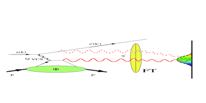
Figure 1: Diagrammatic representation of the “handbag” diagram probed in DVCS; the crossed photon case is omitted. Emission of the final state photon from the target (solid $q^{\prime}$ wave) and lepton beam (dashed $q^{\prime}$ wave) with coherent interference is also shown. A Fourier transform (“FT”) represented by a “lens” creates a probability map of the struck quark probability (shaded) on the transverse spatial image plane.

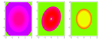
Figure 2: Typical photos, or model images made from transverse position space ($\vec{b}_{T}$) amplitude squared; scale in Fermi. Images made on log-color plots. Left to right: Hofstadter’s rendition; a model with transverse spin, plus a quadratic hole from 3-quark correlations; a proton one-half the size and more concentrated than traditional.

Acknowledgements Work supported in part under Department of Energy Grant. CphT, Ecole Polytechnique is UMR 7644 of CNRS. We acknowledge useful discussions with P. Jain, G. van der Steenhoven, P. Mulders, M. Gar$\cdot$con, M. Diehl, N. D’Hose, P. Kroll, R. Jacob and P. A. M. Guichon.

References

- [1] R. Hofstadter and R. W. Mcallister, Phys. Rev. 98, 217, (1955); R. W. Mcallister and R. Hofstadter, Phys. Rev. 102, 851 (1956); R. Hofstadter, Rev. Mod. Phys. 28, 21, (1956); ibid 30, 482 (1958), with R. Bumiller and M. R. Yearian.
- [2] J. Friedman and W. A Little, Obituary and Biographical Memoire of the National Academy of Science (1990), available in http:// www.nap.edu /readingroom /biomems /rhofstedter.html. For theory typical of the era, see J. J. Sakurai, Advanced Quantum Mechanics (Wiley, 1967), p. 194, which discusses form factors in static approximation.
- [3] D. Müller, D. Robaschik, B. Geyer, F. M. Dittes and J. Hořejši, Fortsch. Phys. 42 (1994) 101; P. Jain and J.P. Ralston, in: Future Directions in Particle and Nuclear Physics at Multi-GeV Hadron Beam Facilities, BNL, March 1993 (hep-ph/9305250); B. Geyer et al., Z. Phys. C26 (1985) 591; T. Braunschweig et al., Z. Phys. C33 (1987) 275; F.-M. Dittes et al., Phys. Lett. B209 (1988) 325; I.I. Balitskii and V.M. Braun, Nucl. Phys. B311 (1988/89) 541; P. Hoodbhoy, hep-ph/9703365; L. Frankfurt et al., Phys. Lett. B418, 345 (1998).
- [4] S. Stepanyan et al. [CLAS Collaboration], Phys. Rev. Lett. 87 (2001) 182002 [arXiv:hep-ex/0107043]; A. Airapetian et al. [HERMES Collaboration], Phys. Rev. Lett. 87 (2001) 182001 [arXiv:hep-ex/0106068].
- [5] X. Ji, Phys. Rev. Lett. 78 (1997) 610; A. V. Radyushkin, Phys. Rev. D56 (1997) 5524.
- [6] R.Buniy, J. P. Ralston, and P. Jain, in VII International Conference on the Intersections of Particle and Nuclear Physics(Quebec City, May 22-28, 2000) edited by Z. Parseh and W. Marciano (AIP, NY 2000); see also DIS 2001: Proceedings of the International Meeting (Bologna, 2001)(World Scientific, in press)
- [7] M. Diehl, T. Gousset, B. Pire and J. P. Ralston, Phys. Lett. B411 (1997) 193.
- [8] D. E. Soper, Phys.Rev. D15, 1141, (1977).
- [9] M. Burkardt, Phys. Rev. D62 071503, 2000; hep-ph/0010082; hep-ph/0008051; hep-ph/0007036. See also A.H Mueller et al Nucl. Phys. B603, 427 (2001) and M. Diehl hep-ph/0205208.
- [10] A. Radyushkin and C. Weiss, Phys. Rev. D63, 114012 (2001).
- [11] S. J. Brodsky, F. E. Close, J.F. Gunion, Phys. Rev. D6, 177 (1972), and Phys. Rev. D5, 1384 (1972).
- [12] A. V. Belitsky et al, Nucl. Phys. B593, 289 (2001) [hep-ph/0004059]; A. V. Belitsky et al, hep-ph/0112108.
- [13] E.R. Berger et al., Phys. Rev. Lett. 87, 142302 (2001).
- [14] S. J. Brodsky, P. Hoyer, N. Marchal, S. Peigne and F. Sannino, Phys. Rev. D 65, 114025 (2002)
- [15] R. G. Arnold, et al, Phys. Rev. Lett. 58, 1723 (1987); P. Bosted, et al, ibid 68, 3841 (1992).
- [16] Presentation speech by Prof. I. Waller, upon the occasion of the Nobel Prize for Physics 1961, the Swedish Academy of Sciences, in Nobel Lectures: Physics 1942-1962(Elsevier, Amseterdam, 1964).