UT-969

hep-ph/0110072

Higgsino and Wino Dark Matter from Q-ball Decay
in Affleck-Dine Baryogenesis

Masaaki Fujii   and   K. Hamaguchi

Department of Physics
University of Tokyo, Tokyo 113-0033, Japan

Supersymmetry (SUSY) has been widely considered as an attractive framework for physics beyond the standard model. It explains the stability of the electroweak scale against quadratically divergent radiative corrections. Furthermore, particle contents of the minimal SUSY standard model (MSSM) lead to a beautiful unification of the three gauge coupling constants of the standard model.

One of the remarkable features in the MSSM is the existence of an ideal dark matter candidate, that is, the lightest SUSY particle (LSP). The most extensively studied LSP as a dark matter candidate is the bino-like neutralino, since its thermal relic abundance naturally provides a desired amount of the present mass density of the dark matter. On the other hand, there have been much less interests in other candidates, such as the Higgsino-like and wino-like neutralino, since their thermal relic densities are generally too low to be a significant component of dark matter [1].

In this letter, we claim that the Higgsino-like and wino-like neutralinos are good dark matter candidates in spite of their large annihilation cross sections, if the origin of the observed baryon asymmetry lies in the Affleck-Dine (AD) baryogenesis [2, 3]. In AD mechanism, a linear combination of squark and/or slepton fields ($\phi$ field) has a large expectation value along a flat direction during an inflationary stage, and its subsequent coherent oscillation creates a large net baryon asymmetry. The coherent oscillation of the $\phi$ field is generally unstable with spatial perturbation and it fragments [4, 5, 6] into non-topological solitons [7], Q-balls. It has been, in fact, shown in detailed numerical calculations [8] that almost all of the initial baryon asymmetry carried by the $\phi$ field is absorbed into the Q-balls.

The Q-ball has a long lifetime and its decay temperature is likely to be well below the freeze-out temperature of the LSP, which leads to the non-thermal production of the dark matter [6]. We show that in the case of the Higgsino-like or wino-like LSP the late-time Q-ball decay and subsequent pair annihilations of the LSP’s naturally give rise to a desired dark-matter energy density. It is very encouraging that such candidates are much more easily detected than the standard bino-like neutralino. As we will see later, the detection rate is in fact more than ten times larger compared with the case of bino-like LSP [13].

Let us first estimate the present energy density of the non-thermally produced LSP. Suppose that there is a non-thermal production of LSP at temperature $T=T_{d}$, where $T_{d}$ is below the freeze-out temperature $T_{f}$ of the LSP. ($T_{f}$ is typically given by $T_{f}\sim m_{\chi}/20$, where $m_{\chi}$ is the mass of the LSP.) The subsequent evolution of the number density $n_{\chi}$ of the LSP is described by the following Boltzmann equation:

$$\dot{n}_{\chi}+3Hn_{\chi}=-\left\langle{\sigma v}\right\rangle n_{\chi}^{2}\,,$$ (1)

where the overdot denotes a derivative with time, $H$ is the Hubble parameter of the expanding universe, and $\left\langle{\sigma v}\right\rangle$ is the thermally averaged annihilation cross section of the LSP. Here, we have neglected the effect of the pair production of LSP’s, which is suppressed by a Boltzmann factor $\exp(-m_{\chi}/T)$ for $T<m_{\chi}$. It is useful to rewrite the above equation in terms of temperature $T$ and number density of LSP per comoving volume $Y_{\chi}\equiv n_{\chi}/s$, where $s=(2\pi^{2}/45)g_{*}T^{3}$ is the entropy density and $g_{*}$ is the effective number of relativistic degrees of freedom. Here and hereafter, we assume that the energy density of the LSP is much smaller than that of the radiation $\rho_{rad}$ at $T\simeq T_{d}$, and no extra entropy production occurs after that. (We will justify this assumption later in the case of Q-ball decay.) Then, we obtain

$$\frac{dY_{\chi}}{dT}=\sqrt{\frac{8\pi^{2}g_{*}}{45}}\left(1+\frac{T}{3g_{*}}\frac{dg_{*}}{dT}\right)\left\langle{\sigma v}\right\rangle M_{pl}Y_{\chi}^{2}\,,$$ (2)

where $M_{pl}=2.4\times 10^{18}~{}\mbox{GeV}$ is the reduced Planck scale. This equation can be analytically solved by using approximations $g_{*}(T)\simeq g_{*}(T_{d})\simeq const$ and $\left\langle{\sigma v}\right\rangle(T)\simeq const$, which results in

$$Y_{\chi}(T)\simeq\left[\frac{1}{Y_{\chi}(T_{d})}+\sqrt{\frac{8\pi^{2}g_{*}(T_{d})}{45}}\left\langle{\sigma v}\right\rangle M_{pl}(T_{d}-T)\right]^{-1}\,.$$ (3)

Therefore, for sufficiently large initial abundance $Y_{\chi}(T_{d})$, the final abundance $Y_{\chi 0}$ for $T\ll T_{d}$ is given by

$$Y_{\chi 0}\simeq\left[\sqrt{\frac{8\pi^{2}g_{*}(T_{d})}{45}}\left\langle{\sigma v}\right\rangle M_{pl}T_{d}\right]^{-1}\,.$$ (4)

Notice that the final abundance $Y_{\chi 0}$ is determined only by the temperature $T_{d}$ and the cross section $\left\langle{\sigma v}\right\rangle$, independently of the initial value $Y_{\chi}(T_{d})$ as long as $Y_{\chi}(T_{d})\gg Y_{\chi 0}$. From the above formula, we obtain the relic mass density of the LSP in the present universe:

$$\Omega_{\chi} \simeq 0.5\left(\frac{0.7}{h}\right)^{2}\times\left(\frac{m_{\chi}}{100~{}\mbox{GeV}}\right)^{3}\left(\frac{10^{-3}}{m_{\chi}^{2}\left\langle{\sigma v}\right\rangle}\right)\times\left(\frac{100~{}\mbox{MeV}}{T_{d}}\right)\left(\frac{10}{g_{*}(T_{d})}\right)^{1/2}\,,$$ (5)

where $h$ is the present Hubble parameter in units of $100\,\,{\rm km}\,\,{\rm sec}^{-1}{\rm Mpc}^{-1}$ and $\Omega_{\chi}\equiv\rho_{\chi}/\rho_{c}$. ($\rho_{\chi}$ and $\rho_{c}$ are the energy density of LSP and the critical energy density in the present universe, respectively.) Notice that the obtained abundance is much larger than the result for thermally produced LSP. In fact, it is enhanced by a factor of $\sim(T_{f}/T_{d})$ compared with the case of standard thermal production with the $s$-wave dominant annihilations.

Now let us discuss the LSP production by the Q-ball decay. First of all, the baryon number density $n_{B}$ is related to the number density of the Q-balls and the initial charge of each Q-ball $Q_{i}$:

$$Q_{i}n_{Q}=fn_{B}\,,$$ (6)

where $f$ denotes the fraction of the total baryon asymmetry which is initially contained in the Q-balls. Notice that almost all the baryon asymmetry is initially stored in the Q-balls [8], namely, $f\simeq 1$.

The decay rate of a single Q-ball is given by [14]:

$$\Gamma_{Q}\equiv-\frac{dQ}{dt}\mathop{}_{\textstyle\sim}^{\textstyle<}\frac{\omega^{3}{\cal A}}{192\pi^{2}}\,,$$ (7)

where $\omega\simeq m_{\phi}$, $m_{\phi}$ is the soft scalar mass of the $\phi$ field, and ${\cal A}$ is the surface area of the Q-ball. (The radius of the Q-ball is given by $R_{Q}\simeq\sqrt{2}|K|^{-1/2}m_{\phi}^{-1}$, where $|K|\simeq 0.01$–$0.1$ [5, 6, 15].) Then, we obtain the lifetime of the Q-ball $\tau_{d}\equiv Q_{i}/\Gamma_{Q}$, or equivalently the decay temperature $T_{d}$ of the Q-ball:

$$T_{d}\mathop{}_{\textstyle\sim}^{\textstyle<}2~{}\mbox{GeV}\left(\frac{0.01}{|K|}\right)^{1/2}\left(\frac{m_{\phi}}{1~{}\mbox{TeV}}\right)^{1/2}\left(\frac{10^{20}}{Q_{i}}\right)^{1/2}\,.$$ (8)

Actually, the formed Q-ball has a large charge and typically decays at $T_{d}\mathop{}_{\textstyle\sim}^{\textstyle<}1~{}\mbox{GeV}$ [6], in particular when the $\phi$ field is lifted by a nonrenormalizable dimension-six operator in the superpotential with a cutoff scale $\sim M_{pl}$. Hereafter, we will take $T_{d}\simeq 10~{}\mbox{MeV}$–$1~{}\mbox{GeV}$. From above equations, the production rate of the LSP per time per volume is given by

$$N_{\chi}\Gamma_{Q}n_{Q} = N_{\chi}\Gamma_{Q}\frac{fn_{B}}{Q_{i}}\theta\left(Q_{i}-\Gamma_{Q}t\right)$$ (9)

$$= N_{\chi}fn_{B}\times\frac{\theta(\tau_{d}-t)}{\tau_{d}}\,,$$

where $N_{\chi}$ is the number of LSP’s produced per baryon number, which is at least $3$. Thus, the evolution of the number density of the LSP is obtained by solving the following equation:

$$\dot{n}_{\chi}+3Hn_{\chi}=N_{\chi}f\left(\frac{n_{B}}{s}\right)_{0}s\times\frac{\theta(\tau_{d}-t)}{\tau_{d}}-\left\langle{\sigma v}\right\rangle n_{\chi}^{2}\,,$$ (10)

where we have normalized the baryon number density by the entropy density and subscript $0$ denotes the present value.

In Eq. (10), it is assumed that the LSP is uniformly distributed. Because the LSP’s are produced from the Q-ball, which is a localized object, one might wonder if the pair annihilation rate of the LSP becomes much larger and its final number density becomes much smaller. However, we can see this is not the case as follows. First of all, it is found from Eq.(3) that the number density of the LSP approaches its final value only after $(T_{d}-T)/T_{d}\sim{\cal O}(1)$, which means it takes a time scale $\Delta t\sim\tau_{d}$. (Notice that this is true for any local number density, as long as it is large enough.) By that time, LSP’s have spread out by a random walk colliding with the background particles, and form a Gaussian distribution around the decaying Q-ball. The central region of this distribution has a radius $\bar{r}\simeq\sqrt{\nu\tau_{d}}$, where $\nu^{-1}\simeq G_{F}^{2}m_{\chi}T_{d}^{4}$ [6]. ($G_{F}$ is the Fermi coupling constant.) Meanwhile, we can see that the number of Q-balls within this radius is much larger than one, roughly given by $(4\pi/3)\,\bar{r}^{3}n_{Q}\sim 10^{10}\times(T_{d}/1\!~{}\mbox{GeV})^{-6}(Q_{i}/10^{20})^{-1}(m_{\chi}/100\!~{}\mbox{GeV})^{-3/2}$. Hence, the assumption of the uniform distribution is justified.

We should also note that the energy density of the Q-balls $\rho_{Q}$ is much smaller than that of the radiation $\rho_{rad}$ for $T\mathop{}_{\textstyle\sim}^{\textstyle>}T_{d}$:

$$\frac{\rho_{Q}}{\rho_{rad}} \simeq \frac{m_{\phi}n_{Q}Q_{i}}{\rho_{rad}}$$ (11)

$$= \frac{3m_{\phi}}{4T}f\left(\frac{n_{B}}{s}\right)_{0}$$

$$\sim 10^{-5}f\times\left(\frac{m_{\phi}}{1~{}\mbox{TeV}}\right)\left(\frac{10~{}\mbox{MeV}}{T}\right)\ll 1\,,$$

where we have used the fact that the energy of the Q-ball per charge is roughly given by $m_{\phi}$. Therefore, no significant entropy production takes place during the Q-ball decay.

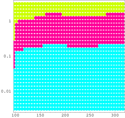
Figure 2: The contour plots of the relic abundance $\Omega_{\chi}$ of the Higgsino-like neutralino LSP in the $m_{\chi}$–$T_{d}$ plane. The parameters are the same as Fig. 1 except $m_{0}=330~{}\mbox{GeV}$. The three shaded regions correspond to the range of $\Omega_{\chi}<0.1$, $0.1<\Omega_{\chi}<1$, $1<\Omega_{\chi}$, from the top to the bottom, respectively.

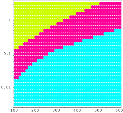
Figure 3: The contour plots of the relic abundance $\Omega_{\chi}$ of the wino-like neutralino LSP in the $m_{\chi}$–$T_{d}$ plane. We took $M_{1}=(3/2)\mu$ and $M_{2}=(1/2)\mu$. Other parameters are the same as Fig. 1. The three shaded regions correspond to the range of $\Omega_{\chi}<0.1$, $0.1<\Omega_{\chi}<1$, $1<\Omega_{\chi}$, from the top to the bottom, respectively.

We have numerically solved the Boltzmann equation (10) for Higgsino-like and wino-like neutralino and calculated the relic abundance $\Omega_{\chi}$, where we have taken $N_{\chi}=3$, $f=1$, $(n_{B}/s)_{0}=0.7\times 10^{-10}$, and $h=0.7$. In our calculation, we included final states; $W^{+}W^{-}$, $ZZ$, $t\bar{t}$, $h^{0}A^{0}$, $H^{0}A^{0}$, $Zh^{0}$, $ZH^{0}$, and $W^{\pm}H^{\mp}$. (We took the cross sections from Ref. [16].) The results are shown in Figs. 1–3 in the $m_{\chi}$–$T_{d}$ plane. Figs. 1 and 2 correspond to the Higgsino-like LSP, where we took $M_{1}=(3/2)\mu$ and $M_{2}=3\mu$, while Fig. 3 corresponds to the wino-like LSP, where we took $M_{1}=(3/2)\mu$ and $M_{2}=(1/2)\mu$. ($M_{1}$ and $M_{2}$ are the soft gaugino masses for the $SU(2)_{L}$ and $U(1)_{Y}$ gauge groups, respectively, and $\mu$ denotes the SUSY contribution to the Higgs-boson (Higgsino) masses.) As for the other parameters, we used $\tan\beta=5$, $m_{A^{0}}=300~{}\mbox{GeV}$ and all trilinear scalar couplings $a=0$, in all figures. For sfermions we assumed universal soft masses $m_{\widetilde{f}i}=m_{0}$. We used $m_{0}=1~{}\mbox{TeV}$ in Figs.1 and 3, and $m_{0}=330~{}\mbox{GeV}$ in Fig.2. We used the $g_{*}(T)$ given in Ref. [17] for $100~{}\mbox{MeV}\mathop{}_{\textstyle\sim}^{\textstyle<}T\mathop{}_{\textstyle\sim}^{\textstyle<}1~{}\mbox{GeV}$, adopting the QCD phase transition near $150~{}\mbox{MeV}$.

It is found from these figures that both of the the mass densities of the Higgsino-like and wino-like LSP in fact fall in the desired region $\Omega_{\chi}\simeq 0.1$–$1$ in a wide range of LSP mass, for Q-ball decay temperatures $T_{d}\simeq 10~{}\mbox{MeV}$–$1~{}\mbox{GeV}$. (We have also confirmed that these results are well reproduced by the analytic calculation given in Eq. (5).) It is remarkable that the Higgsino-like and the wino-like LSP’s can be excellent dark matter candidates even in the relatively small mass region, where the thermal production would give rise to too small relic abundance. (See discussion below Eq.(5).) As we will see later, these regions are also advantageous for dark matter search experiments.

Here, we should note that the Q-ball decay would produce too large amount of dark matter density if there were no pair annihilation of the LSP’s. This can be easily seen by integrating the Eq. (10) with $\left\langle{\sigma v}\right\rangle=0$:

$$\left.\Omega_{\chi}\right|_{\rm no\,\,ann} = 3\left(\frac{N_{\chi}}{3}\right)f\left(\frac{m_{\chi}}{m_{n}}\right)\Omega_{B}$$ (12)

$$\mathop{}_{\textstyle\sim}^{\textstyle>} 2.6\,f\times\left(\frac{N_{\chi}}{3}\right)\left(\frac{m_{\chi}}{100~{}\mbox{GeV}}\right)\left(\frac{0.7}{h}\right)^{2}\,,$$

where $m_{n}\simeq 1~{}\mbox{GeV}$ is the nucleon mass, and we have used the bound on the present baryon density $\Omega_{B}h^{2}\mathop{}_{\textstyle\sim}^{\textstyle>}0.004$ [18]. Therefore, in the case of the bino-like LSP, the Q-ball formation is a serious obstacle for the AD baryogenesis. (Detailed discussion on this problem and possible solutions are given in Ref. [11].)

As we have seen, Higgsino-like and wino-like LSP are promising candidates for cold dark matter if the AD baryogenesis is responsible for generating the observed baryon asymmetry in the present universe. Encouragingly enough, if this is the case, the direct detecting possibility for these dark matter is enormously enhanced compared with the case of bino-like dark matter [19, 13].

The relevant quantity for direct search experiments is the elastic neutralino-nucleon scattering rate [20]:

$$R=\frac{\sigma\rho_{\chi}^{halo}v_{\chi}F_{\xi}}{m_{\chi}M_{N}},$$ (13)

where $\rho_{\chi}^{halo}$ and $v_{\chi}$ is the mass density and the average speed of the neutralinos in the galactic halo, respectively. $M_{N}$ is the mass of the target nucleus, and $F_{\xi}$ is the nuclear form factor. By using typical values, this scattering rate is written as

$$R=\frac{\sigma F_{\xi}}{m_{\chi}M_{N}}\;1.8\times 10^{11}~{}\mbox{GeV}^{4}\;\left(\frac{\rho_{\chi}^{halo}}{0.3~{}\mbox{GeV}/\mbox{cm}^{3}}\right)\left(\frac{v_{\chi}}{320\mbox{km/sec}}\right)\left(\frac{\mbox{events}}{\mbox{kg}\cdot\mbox{day}}\right).$$ (14)

The list of relevant coupling constants are given in Ref. [20]. For the numerical calculations in this work, we have neglected the squark and Z-boson exchange contributions, since they are subdominant components in most of the parameter space [13], and we have taken $F_{\xi}=1$ for simplicity.

In Fig. 4 and 5, we show the scattering rates for the Higgsino-like and wino-like dark matter in ${}^{76}Ge$ detector, respectively. In these calculations, we have taken the same parameter sets as in Fig. 1 and 3 except $\tan\beta$. From these figures, we see that the detection rates for the Higgsino-like and wino-like dark matter are $R\geq 0.01\;\mbox{events}/\mbox{kg}\cdot\mbox{day}$ in very wide range of parameter space, and they even reach $R\geq 0.1\;\mbox{events}/\mbox{kg}\cdot\mbox{day}$ in the large $\rm{tan}\beta$ region. We should stress that such a parameter region where $R\geq 0.01\;(\mbox{events}/\mbox{kg}\cdot\mbox{day})$ is within the reach of the on-going cold dark matter searches [21].

For comparison, we also show the scattering rate in ${}^{76}Ge$ detector for the case of bino-like dark matter in Fig. 6. Here, we have taken $M_{1}=(1/3)\mu,\;M_{2}=(2/3)\mu$, and other parameters are the same as in Fig. 4 and 5. As we noted, the scattering rate for the bino-like dark matter is much smaller than Higgsino-like and wino-like dark matter, and the direct detection in the dark matter search experiments is much more difficult.

To summarize, we pointed out in this letter that the Higgsino-like and wino-like LSP’s can be excellent dark matter candidates if the Affleck-Dine baryogenesis is responsible for the generation of the observed baryon asymmetry in the present universe. Actually, we showed that the relic abundances of these LSP’s can naturally explain the observed dark matter density with natural Q-ball decay temperatures, even in the relatively light neutralino mass region, which is much advantageous for the direct dark matter searches [21].

The novel thermal history of the universe proposed in this letter may have important implications on general SUSY breaking models, which include mSUGRA, no-scale type models with non-universal gaugino masses [22], anomaly mediated SUSY breaking model [23], and so on. Detailed analysis on specific models will be given elsewhere [24].

In the context of the anomaly-mediated SUSY breaking (AMSB) [23], non-thermal production of the wino dark matter from the late time decay of moduli and gravitino was investigated in Ref. [19]. In the case of moduli decay, however, there exists large entropy production which substantially dilutes the primordial baryon asymmetry. The authors suggested that the AD baryogenesis can produce enough baryon asymmetry even in this case. Although the AD mechanism in AMSB scenario is generally difficult, there is an attractive AD scenario [11] which naturally works even in AMSB. However, if there is a large entropy production from the moduli decay, it is highly difficult to generate the required baryon asymmetry. Even if this is possible, the decay of the resultant large Q-ball probably plays a comparable role with the moduli decay as the non-thermal source of the LSP’s.

Figure 1: The contour plots of the relic abundance $\Omega_{\chi}$ of the Higgsino-like neutralino LSP in the $m_{\chi}$–$T_{d}$ plane. We have taken $h=0.7$, $M_{1}=(3/2)\mu$, $M_{2}=3\mu$, $\tan\beta=5$, $m_{A^{0}}=300~{}\mbox{GeV}$, $a=0$, and $m_{0}=1~{}\mbox{TeV}$. The three shaded regions correspond to the range of $\Omega_{\chi}<0.1$, $0.1<\Omega_{\chi}<1$, $1<\Omega_{\chi}$, from the top to the bottom, respectively.

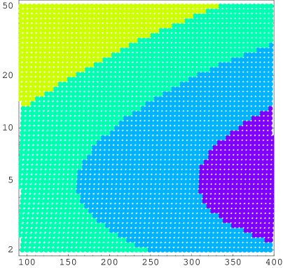
Figure 4: Contours of the detection rate for the Higgsino-like dark matter in ${}^{76}Ge$ detector. The four shaded regions correspond to the ranges of the detection rate $R>0.1$, $0.1\geq R>0.03$, $0.03\geq R>0.01$, $0.01\geq R\;\;(\mbox{events}/\mbox{kg}\cdot\mbox{day})$ from left to right, respectively. The parameters used in this calculation are the same as in Fig. 1 except $\tan\beta$.

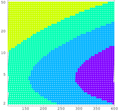
Figure 5: Contours of the detection rate for the wino-like dark matter in ${}^{76}Ge$ detector. The four shaded regions correspond to the ranges of the detection rate $R>0.1$, $0.1\geq R>0.03$, $0.03\geq R>0.01$, $0.01\geq R\;\;(\mbox{events}/\mbox{kg}\cdot\mbox{day})$ from left to right, respectively. The parameters used in this calculation are the same as in Fig. 3 except $\tan\beta$.

Figure 6: Contours for the detection rate for the bino-like dark matter in ${}^{76}Ge$ detector. The four shaded regions correspond to the ranges of the detection rate $0.03\geq R>0.01$, $0.01\geq R>0.003$, $0.003\geq R>0.001$, $0.001\geq R\;\;(\mbox{events}/\mbox{kg}\cdot\mbox{day})$ from left to right, respectively. Here we have taken $M_{1}=(1/3)\mu$ and $M_{2}=(2/3)\mu$. Other parameters are the same as in Fig. 4 and 5.

References

-
[1]
S. Mizuta and M. Yamaguchi,
Phys. Lett. B 298 (1993) 120
[arXiv:hep-ph/9208251];
S. Mizuta, D. Ng and M. Yamaguchi, Phys. Lett. B 300 (1993) 96 [arXiv:hep-ph/9210241]; - [2] I. Affleck and M. Dine, Nucl. Phys. B 249 (1985) 361.
- [3] M. Dine, L. J. Randall and S. Thomas, Nucl. Phys. B 458 (1996) 291 [arXiv:hep-ph/9507453].
- [4] A. Kusenko and M. E. Shaposhnikov, Phys. Lett. B 418 (1998) 46 [arXiv:hep-ph/9709492].
- [5] K. Enqvist and J. McDonald, Phys. Lett. B 425 (1998) 309 [arXiv:hep-ph/9711514];
- [6] K. Enqvist and J. McDonald, Nucl. Phys. B 538 (1999) 321 [arXiv:hep-ph/9803380].
- [7] S. R. Coleman, Nucl. Phys. B 262 (1985) 263 [Erratum-ibid. B 269 (1985) 744].
-
[8]
S. Kasuya and M. Kawasaki,
Phys. Rev. D 61 (2000) 041301
[hep-ph/9909509];
S. Kasuya and M. Kawasaki, Phys. Rev. D 62 (2000) 023512 [hep-ph/0002285]. -
[9]
M. Dine, A. E. Nelson and Y. Shirman,
Phys. Rev. D 51 (1995) 1362
[hep-ph/9408384];
M. Dine, A. E. Nelson, Y. Nir and Y. Shirman, Phys. Rev. D 53 (1996) 2658 [hep-ph/9507378];
For a review, see, for example, G. F. Giudice and R. Rattazzi, Phys. Rept. 322 (1999) 419 [hep-ph/9801271]. - [10] G. R. Dvali, A. Kusenko and M. E. Shaposhnikov, Phys. Lett. B 417 (1998) 99 [arXiv:hep-ph/9707423].
- [11] M. Fujii, K. Hamaguchi and T. Yanagida, arXiv:hep-ph/0104186, to appear in Phys. Rev. D.
- [12] J. McDonald, JHEP 0103 (2001) 022 [arXiv:hep-ph/0012369].
- [13] B. Murakami and J. D. Wells, hep-ph/0011082.
- [14] A. G. Cohen, S. R. Coleman, H. Georgi and A. Manohar, Nucl. Phys. B 272 (1986) 301.
- [15] K. Enqvist, A. Jokinen and J. McDonald, Phys. Lett. B 483 (2000) 191 [arXiv:hep-ph/0004050].
- [16] M. Drees and M. M. Nojiri, Phys. Rev. D 47 (1993) 376 [arXiv:hep-ph/9207234].
- [17] M. Srednicki, R. Watkins and K. A. Olive, Nucl. Phys. B 310 (1988) 693.
- [18] K. A. Olive, G. Steigman and T. P. Walker, Phys. Rept. 333 (2000) 389 [arXiv:astro-ph/9905320].
- [19] T. Moroi and L. J. Randall, Nucl. Phys. B 570 (2000) 455 [hep-ph/9906527].
- [20] M. Drees and M. Nojiri, Phys. Rev. D 48 (1993) 3483 [arXiv:hep-ph/9307208].
- [21] G. Jungman, M. Kamionkowski and K. Griest, Phys. Rept. 267 (1996) 195 [arXiv:hep-ph/9506380].
- [22] S. Komine and M. Yamaguchi, Phys. Rev. D 63 (2001) 035005 [arXiv:hep-ph/0007327].
-
[23]
L. J. Randall and R. Sundrum,
Nucl. Phys. B 557 (1999) 79
[hep-th/9810155];
G. F. Giudice, M. A. Luty, H. Murayama and R. Rattazzi, JHEP 9812 (1998) 027 [hep-ph/9810442];
J. A. Bagger, T. Moroi and E. Poppitz, JHEP 0004 (2000) 009 [arXiv:hep-th/9911029]. - [24] M. Fujii and K. Hamaguchi, in preparation.