Isospin Fluctuations in QCD and Relativistic Heavy-Ion Collisions

Abstract

We address the role of fluctuations in strongly interacting matter during the dense stages of a heavy-ion collision through its electromagnetic emission. Fluctuations of isospin charge are considered in a thermal system at rest as well as in a moving hadronic fluid at fixed proper time within a finite bin of pseudo-rapidity. In the former case, we use general thermodynamic relations to establish a connection between fluctuations and the space-like screening limit of the retarded photon self-energy, which directly relates to the emissivities of dileptons and photons. Effects of hadronic interactions are highlighted through two illustrative calculations. In the latter case, we show that a finite time scale $\tau$ inherent in the evolution of a heavy-ion collision implies that equilibrium fluctuations involve both space-like and time-like components of the photon self-energy in the system. Our study of non-thermal effects, explored here through a stochastic treatment, shows that an early and large fluctuation in isospin survives only if it is accompanied by a large temperature fluctuation at freeze-out, an unlikely scenario in hadronic phases with large heat capacity. We point out prospects for the future which include: (1) A determination of the Debye mass of the system at the dilute freeze-out stage of a heavy-ion collision, and (2) A delineation of the role of charge fluctuations during the dense stages of the collision through a study of electromagnetic emissivities.

PACS: 12.38.Mh, 25.75.-q, 13.40.-f, 24.10.Nz

]

I INTRODUCTION

Charge fluctuations extracted through event-by-event measurements in high-energy heavy-ion collisions have recently attracted attention as a potential signature of Quark-Gluon Plasma (QGP) formation [1]. In the confined phase charges are carried by hadrons in integer units of $e$, while in the deconfined phase they are attached to quarks in fractional units. This leads to charge fluctuations and associated thermodynamic susceptibilities that are distinctly different in the two phases [2]. If significant primordial fluctuations survive the evolution of the collision, one might hope to deduce the properties of deconfined matter at the early stages, analogous to the manner in which primordial fluctuations in the early universe are inferred through the detection of anisotropy in the cosmic background radiation. Beginning with the expected signals in rapidity distributions [3], many sources and signals of fluctuations in hadronic observables have been considered (cf. [4] and references therein). For more recent discussions, see, for example, Refs. [5, 6, 7, 8].

In experiments at the CERN SPS and RHIC to date, observed fluctuations in hadronic multiplicities, kaon to pion ratios, and transverse momenta agree reasonably well with model calculations of these quantities at the dilute freeze-out stage of the system [4]. Such studies, however, have not unraveled the physics associated with the QGP phase transition. Whether future collider experiments at RHIC and LHC will reveal tell-tale signatures in fluctuations of hadronic observables alone remains to be seen.

It must be noted that the measured fluctuations in hadronic observables result from a combination of several factors that include: (1) The evolution of the created system from a dense partonic stage to a dilute hadronic stage. The duration of each stage is especially critical inasmuch as the memory of the partonic stage is more likely to be retained by the hadrons provided the hadronic stage is of relatively short duration; and (2) The extent to which interactions are different in the two phases. A caveat, of course, is that if duality between the partonic and hadronic worlds holds, equivalent descriptions of observables may be achieved by considering interactions in the two phases. A good example is provided by the cross sections ratio $R=\sigma_{e^{+}e^{-}\to hadrons}/\sigma_{e^{+}e^{-}\to\mu^{+}\mu^{-}}$ for $\sqrt{s}\mathrel{\raise 1.29167pt\hbox{$>$\kern-7.5pt\lower 4.30554pt\hbox{$\sim$}}}1.5$ GeV; in this case, interacting hadronic states yield a description that is equivalent to one that involves perturbative quarks and gluons.

Our principal objective in this paper is to emphasize that possibly the only way to address the role of fluctuations during the dense stages of the collision is to exploit electromagnetic probes in combination with hadronic probes. Towards this goal, we study relations between electromagnetic radiation and thermal fluctuations of isospin charge in a system at rest as well as in an expanding hadronic fluid at fixed proper time and in appropriately chosen bins of pseudo-rapidity.

For a system at rest, we utilize general thermodynamic relations to establish connections between fluctuations in matter and the space-like screening limit of the retarded photon self-energy, a quantity which directly controls the thermal emissivities of dileptons and photons. We consider two examples that exemplify the effects of hadronic interactions on electromagnetic radiation. In addition, we point out the close connections that exist between fluctuations, susceptibilities, and average phase space densities. At the dilute freeze-out stage, the average phase space densities of pions and kaons can be inferred through interferometric (Hanbury-Brown and Twiss) studies [9, 10] and provide for a direct determination of the system’s Debye mass.

For a system undergoing relativistic expansion, we derive a general formula for fluctuations in isospin charge binned in pseudo-rapidity intervals of width $\Delta$. The constituents of the moving fluid, be they partons or hadrons, are assumed to be in local thermal equilibrium. In the case of hadrons, we include finite pion and baryon chemical potentials. We cast our result in a readily usable form for the analysis of experiments, which have unavoidable restrictions in rapidity and transverse momenta due to limited acceptance in these variables. We show that finite time scales $\tau$ inherent in heavy-ion collisions imply that equilibrium fluctuations involve both space-like and time-like components of the photon’s polarization function with predominant contributions arising from frequency $f\approx 2\pi/\tau$ and wavelength $\lambda\approx\pi\tau\,{\rm sh}(\Delta/2)$. We also consider effects of non-equilibrium (for previous work, see for example, Ref. [11]) with a view to explore the consequences of possible temperature fluctuations at the freeze-out stage.

This article is organized as follows. In Sec. II, the relationship between isospin fluctuations and space-like physics that leads to screening of charges is established in an infinite volume system at rest and in thermal equilibrium. Secs. II.A through II.D briefly summarize known relations that have enabled us to interrelate fluctuations, susceptibilities, and average phase space densities. In Sec. II.E, connections to electromagnetic (dilepton and photon) emissivities are set up. Two illustrative calculations incorporating effects of hadronic interactions in the dilepton and photon emission rates are presented in Sec. II.F. In Sec. III A, the role of fluctuations in heavy-ion collisions, in which the system created expands from an initially dense partonic system to a dilute hadronic system prior to freeze-out, is discussed with particular emphasis on electromagnetic probes. We demonstrate that in a relativistically expanding fluid, thermal fluctuations probe both space-like (screening) and time-like (emission) physics (Sec. III A). A discussion that relates our findings to those in earlier works is contained in Sec. III B. In Sec. IV, we show how isospin fluctuations present in the early stage can only survive if a sizable temperature fluctuation is simultaneously present at freeze-out. This section contains an analysis of non-equilibrium effects treated stochastically through additive Gaussian and multiplicative power-law heat flow. Our summary and conclusions are contained in Sec. V.

II THERMALLY EQUILIBRATED SYSTEM AT REST

A Fluctuations

We begin by considering a system of infinite spatial 3-volume $V_{3}$ at rest and in thermal equilibrium. The isospin charge operator, ${{\cal Q}}^{a}$, is obtained from the zeroth component of the pertinent current, ${{\cal V}}_{\mu}^{a}$, through

$${{\cal Q}}^{a}(0)=\int\,\,d^{3}x\,{{\cal V}}_{0}^{a}(0,\vec{x})=\int\,\,d^{3}x\,\,\bar{q}(x)\,\gamma_{0}\,\frac{\tau^{a}}{2}\,{q}(x)\ ,$$ (1)

where $q$ denotes quark-field operators and $\vec{\tau}$ are the standard $SU(2)$ isospin matrices (here and in what follows calligraphic letters indicate operators). The thermal fluctuations are defined by

$$\Delta Q^{2} \equiv \left\langle{{\cal Q}}^{a}(0)\,{{\cal Q}}^{a}(0)\right\rangle_{c}$$ (2)

$$= \int d^{3}xd^{3}x^{\prime}\left\langle{{\cal V}}_{0}^{a}(0,x)\,{{\cal V}}_{0}^{a}(0,x^{\prime})\right\rangle_{c}$$ (3)

$$= V_{3}\int d^{3}x\left\langle{{\cal V}}_{0}^{a}(0,x)\,{{\cal V}}_{0}^{a}(0,0)\right\rangle_{c}$$ (4)

$$= V_{3}\ \frac{1}{\beta}\ i\int d^{3}x\int dx^{0}\theta(x^{0})\left\langle[{{\cal V}}_{0}^{a}(x),{{\cal V}}_{0}^{a}(0)]\right\rangle\,,$$ (5)

where

$$\langle{\cal O}\rangle\equiv{\rm Tr}\,\left[{\rm e}^{-\beta({\cal H}-\mu{\cal Q}-\Omega)}{\cal O}\right]$$ (6)

indicates the thermal expectation value of the operator ${\cal O}$. The subscript $c$ in $\langle\cdots\rangle$ refers to connected parts. The relevant chemical potential is denoted by $\mu$, $\beta=1/T$ is the inverse temperature, and $\Omega$ is the thermodynamic potential. The last line in Eq. (5) follows from general analytic properties of the retarded correlator with the order of integration fixed to enforce approach from the space-like regime.

B Susceptibilities

The local fluctuations in a globally conserved quantity can be expressed through a derivative of the thermal expectation value of ${\cal O}$ with respect to the associated chemical potential (see, e.g., Refs. [12, 13]):

$$(\Delta{\cal O})^{2}=\langle{\cal O}^{2}\rangle-\langle{\cal O}\rangle^{2}=-T\frac{\partial\langle{\cal O}\rangle}{\partial\mu}\ .$$ (7)

Since the charge-density is defined as a partial derivative of the thermodynamic potential, its thermal fluctuations are given by the charge susceptibility

$$\chi_{ch}\equiv\frac{1}{V_{3}}\frac{\partial^{2}\Omega}{\partial\mu_{ch}^{2}}=\frac{(\Delta Q)^{2}}{TV_{3}}\ .$$ (8)

A general relation between the susceptibility and the $00$-component of the electromagnetic (e.m.) polarization tensor is (see, e.g., Refs. [2, 14, 15, 16])

$$\chi_{ch}\equiv-\Pi^{00}(q_{0}=0,\vec{q}\to 0)=m_{D}^{2}\ ,$$ (9)

where $m_{D}$ is the Debye mass (strictly speaking, this relation is valid only to leading order in $e^{2}$). Equation (9), also implied by Eq. (5), then provides a direct link to the electric screening length in the system. On kinematical grounds, one expects $m_{D}^{2}(T)$ to receive contributions chiefly from low-lying mesonic excitations in a hadronic gas and from (nearly) massless quarks and anti-quarks in a partonic gas.

C Examples in Hadronic and Quark-Gluon-Plasma Phases

We turn now to estimates of charge fluctuations assuming thermal equilibrium (this assumption is relaxed later in Sec. IV). A meaningful quantity accessible to experiments is the magnitude of the hadronic fluctuations normalized to the entropy $S$ in a suitable subvolume $V_{3}$ of the system (realized, e.g., via a restricted rapidity interval of data):

$$R=\frac{(\Delta Q)^{2}}{S}=\frac{(\Delta Q)^{2}/V_{3}}{S/V_{3}}=\frac{Tm_{D}^{2}}{s}\ ,$$ (10)

where $s$ is the entropy-density. In the ideal gas approximation,

$$(m_{D}^{0})^{2}=\beta\sum\limits_{i}d_{i}^{ch}\int\frac{d^{3}k}{(2\pi)^{3}}\ f(\omega_{i})\ [1\mp f(\omega_{i})]$$ (11)

and

$$s=\mp\sum\limits_{i}d_{i}\int\frac{d^{3}k}{(2\pi)^{3}}[ \pm f(\omega_{i})\ln f(\omega_{i})$$ (12)

$$+ (1\mp f(\omega_{i}))\ln(1\mp f(\omega_{i})]\,,$$ (13)

where the summations run over all particle species $i$; the upper (lower) sign refers to fermions (bosons), $d_{i}^{ch}\equiv d_{i}^{spin}\ \sum_{I_{3}}(q_{i}^{I_{3}})^{2}$ denotes the (squared) charge degeneracy of a given isospin-multiplet, $d_{i}$ is the corresponding total degeneracy, and $\omega_{i}^{2}=m_{i}^{2}+k^{2}$. The thermal distribution functions $f=f^{B}$ or $f^{F}$ correspond to bosons or fermions, respectively. It is important to note that, despite their simplicity, Eqs. (11) and (13) take account of interactions between the hadrons to the extent that the thermodynamics of an interacting system of hadrons can be approximated by that of a mixture of ideal gases of “elementary” particles and their resonances (cf. [17] and references therein).

For a massless pion gas, $R_{\pi}^{0}=0.253$. With the empirical vacuum pion mass, $R^{id}_{\pi}(T_{chem})\cong 0.18$ at a typical chemical freeze-out temperature $T_{chem}\cong 180$ MeV. As pointed out in Ref. [5], inclusion of higher-mass hadronic resonances reduces this number further to $R^{id}_{HG}\cong 0.06-0.07$. This is readily understood from the fact that heavier particles give relatively larger contributions to the entropy density than they do to the susceptibility (see Eqs. (11) and (13)).

In contrast, in a non-interacting QGP with 2 massless flavors and $N_{c}$ colors, $R_{QGP}$=$\frac{1}{3}N_{c}\frac{5}{9}/(37\times 4\pi^{2}/90)$=0.034. Perturbative calculations to higher order in the strong coupling constant can be found, e.g., in Ref. [18]. The use of nonperturbative results from lattice gauge simulations [19] to extract information on the electromagnetic susceptibility has been alluded to, e.g., in Ref. [6]. As expected, the fluctuations in a QGP at temperatures $T\gg T_{c}$ seem to be rather close to the naive perturbative result. Close to $T_{c}$, the situation is less clear.

D Average Phase Space Densities

Liouville’s theorem guarantees that the final state average phase space density of a system gets frozen at a certain time and gives a measure of the dynamics in the prior interacting stage. As observed in Ref. [9], interferometric (Hanbury-Brown and Twiss) studies of particle correlations provide a measure of the average phase space density of the particles in the final state. We add here that such knowledge also provides for a determination of the Debye mass. This is easily seen by recasting Eq. (11) for the squared Debye mass to read as

$$(m_{D}^{0})^{2} = \frac{n_{ch}}{T}\left[1\mp\langle f\rangle_{ch}\right]\,,\quad{\rm or}$$ (14)

$$\langle f\rangle_{ch} = \mp\left[\frac{T(m_{D}^{0})^{2}}{n_{ch}}-1\right]\,,$$ (15)

where $n_{ch}$ is the total number density of charged particles and $\langle f\rangle_{ch}$ is the average phase space density of all charged particles. To the extent that $n_{ch},T$, and $\langle f\rangle_{ch}$ can be determined from experiments, at least at the dilute freeze-out stage of a heavy-ion collision, an estimate of the Debye mass is rendered possible from Eq. (14). Equation (15) is also useful, insofar as it provides a consistency check on models that predict the Debye mass from first principles [20].

For a single species of bosons or fermions, the average phase space density may be expressed as

$$\langle f\rangle=\int\frac{d^{3}k}{(2\pi)^{3}}\,f^{2}\bigg{/}\int\frac{d^{3}k}{(2\pi)^{3}}\,f\qquad\qquad$$ (16)

$$=\frac{\sum\limits_{j=1}^{\infty}(\pm)^{j+1}\left(\frac{j}{j+1}\right)\exp[(j+1)\beta\mu]~{}K_{2}[(j+1)\beta m]}{\sum\limits_{j=1}^{\infty}(\pm)^{j+1}\left(\frac{1}{j}\right)\exp[j\beta\mu]~{}K_{2}[j\beta m]},$$ (17)

where the $+(-)$ sign refers to bosons (fermions) and $K_{2}(x)$ is a modified Bessel function. For temperatures such that $T/m\ll 1$, use of the asymptotic relation $K_{\nu}(x)\sim(\pi/2x)^{1/2}~{}\exp(-x)$ reduces Eq. (17) to the result

$$\langle f^{B,F}\rangle\simeq\frac{\exp[\beta(\mu-m)]}{(2\sqrt{2})}\,,$$ (18)

which is valid in the classical regime.

For orientation, we show in Fig. 1 results for the average phase space density $\langle f^{B}\rangle_{ch}$ of charged pions and kaons for selected values of their respective chemical potentials as functions of temperature. Although results for temperatures up to 200 MeV are shown in this figure for illustrative purposes, we should focus our attention on temperatures below $T_{c}$, the temperature at which the transition to a QGP phase occurs. For reference, the dotted line in the upper panel shows the result $\langle f^{B}\rangle_{ch}\simeq 0.37$ for massless pions at zero chemical potential (in contrast, $\langle f^{F}\rangle_{ch}\simeq 0.088$ for massless fermions at zero chemical potential). All other curves show results with vacuum values of masses. The dashed curves in both panels are for zero chemical potentials. Evident features from the results of this figure are: (1) Increasing masses of bosons reduce $\langle f\rangle_{ch}$; (2) Positive (negative) chemical potentials of bosons enhance (suppress) $\langle f^{B}\rangle_{ch}$ relative to its value at $\mu=0$. For chemical potentials approaching the mass of the particle (incipient Bose condensation), the average phase space occupancy begins to become increasingly large; and (3) The higher (lower) the temperature, the higher (lower) is $\langle f^{B}\rangle_{ch}$.

FIG. 1.: Average phase space densities $\langle f^{B}\rangle_{ch}$ of charged pions (upper panel) and kaons (lower panel) as functions of temperature at the indicated values of their respective chemical potentials. The dotted curve in the upper panel shows $\langle f^{B}\rangle_{ch}\simeq 0.37$ for massless pions at zero chemical potential.

It is straightforward to compute $\langle f\rangle_{ch}$ in a mixture of hadrons through the use of Eq. (17) by summing over the various species with their appropriate charge degeneracies $d_{i}^{ch}$. We refer the reader to Refs. [9, 10], where the extent to which the conditions at the freeze-out stage of the collision can be delimited are discussed.

E Electromagnetic Correlations

An intimate connection exists between the fluctuations of the charged constituents in the system and the emission of electromagnetic radiation. The e.m. polarization tensor figuring in Eq. (9) directly governs the production rates of dileptons and photons. This is important, since electromagnetic emission occurs throughout the evolution of the system created in heavy-ion collisions and ranks highly among the principal ways in which the dense stages of evolution can be directly probed (cf. [21] and references therein).

Beginning with dilepton ($l^{+}l^{-}$) emission, we note that the rate of production from a thermally equilibrated system is given by

$$\frac{dR_{l^{+}l^{-}}}{d^{4}q} = L^{\mu\nu}(q)\ W_{\mu\nu}^{{\rm em}}(q)$$ (19)

$$= -\frac{\alpha^{2}}{\pi^{3}M^{2}}f^{B}(q_{0};T)\frac{1}{3}\left({\rm Im}\,\Pi^{L}+2{\rm Im}\,\Pi^{T}\right)\,,$$ (20)

where $L^{\mu\nu}$ is the usual lepton tensor, and the electromagnetic hadron tensor

$$W_{\mu\nu}^{{\rm em}}(q)=\int\,d^{4}x\,{\rm e}^{iq\cdot x}\,\left\langle{\cal J}_{\mu}^{{\rm em}}(x)\,\,{\cal J}_{\nu}^{{\rm em}}(0)\right\rangle_{c}$$ (21)

is given directly in terms of the imaginary part of the retarded photon self-energy

$$W_{\mu\nu}^{{\rm em}}=-2~{}f^{B}(q_{0};T)~{}{\rm Im}~{}\Pi_{\mu\nu}\,.$$ (22)

Photon emission rates are obtained by taking the limit $M^{2}\equiv q_{0}^{2}-q^{2}\rightarrow 0$ in the above expressions. Note that, unlike the space-like limit involved in Eq. (9), dilepton (photon) production probes the time-like regime (limit), as well as both the longitudinal and transverse parts of the electromagnetic polarization tensor.

We turn now to elaborate on this interrelation, beginning with the simple and transparent case of an ideal gas of massless constituents (either pions or quarks). In this case, the leading temperature contribution to the one-loop self-energy is (see, e.g., Ref. [18])

$$\Pi^{00}(q_{0},q) = -m_{D}^{2}\ d_{Q}$$ (23)

$$\times \left[1-\frac{q_{0}}{2q}\left(\ln\left|\frac{q_{0}+q}{q_{0}-q}\right|-i\pi\theta(-M^{2})\right)\right]\ ,$$ (24)

where $d_{Q}=1$ ($N_{c}\sum_{q}e_{q}^{2}$) for pions (quarks). Note that $\Pi^{00}(q_{0},q)$ acquires an imaginary part only for space-like $M^{2}<0$, due to Landau damping. The dilepton production rate, which stems from the time-like region characterizing decay contributions (emissivities), takes the form

$$\frac{dR_{l^{+}l^{-}}}{d^{4}q} = \frac{\alpha^{2}\tilde{d}_{Q}}{\pi^{3}M^{2}}f^{B}(q_{0})\ \frac{M^{2}}{48\pi}\left[1+\frac{2T}{q}\ln\left(\frac{x_{+}\mp 1}{x_{-}\mp 1}\right)\right]$$ (25)

$$\stackrel{{\scriptstyle q\to 0}}{{=}} \frac{\alpha^{2}\tilde{d}_{Q}}{\pi^{3}M^{2}}f^{B}(q_{0})\ \frac{M^{2}}{48\pi}\left[1\pm 2f\left(\frac{q_{0}}{2}\right)\right]\ ,$$ (26)

where $\tilde{d}_{Q}=1$ for pions or $N_{s}^{2}N_{c}\sum_{q}e_{q}^{2}$ for quarks ($N_{s}=2$), and $x_{\pm}=\exp[-(q_{0}\pm q)/2T]$.

For illustrative purposes, the $q\to 0$ limit has been taken in the rightmost expression. Note that the overall Bose factor is not part of the photon self-energy so that the leading temperature contribution to dilepton production is due to the imaginary part of the vacuum piece. In the $q\to 0$ limit, the explicit form of the 00-component for time-like $M^{2}>0$ is

$${\rm Im}\,\Pi^{00}(q_{0},q)=-\frac{q^{2}}{12\pi}\left[1\pm 2f\left(\frac{q_{0}}{2}\right)\right]\ .$$ (27)

A formal connection between the space-like and time-like regimes can, in principle, be constructed via a dispersion relation. For the case of interest here, the analytic properties of the retarded photon self-energy imply that

$${\rm Re}\,\Pi^{00}(q_{0}=0,q)=-\int\limits_{0}^{\infty}\frac{d\omega^{2}}{\pi}\frac{{\rm Im}\,\Pi^{00}(\omega,q)}{-(\omega^{2})}\qquad\qquad$$ (28)

$$\quad=-\int\limits_{0}^{q}\frac{d\omega^{2}}{\pi}\frac{{\rm Im}\,\Pi^{00}(\omega,q)}{-(\omega^{2})}-\int\limits_{q}^{\infty}\frac{d\omega^{2}}{\pi}\frac{{\rm Im}\,\Pi^{00}(\omega,q)}{-(\omega^{2})}\ ,$$ (29)

where the second equality explicitly shows the decomposition into space-like and time-like contributions. Using the imaginary parts from Eqs. (24) and (27), we find that ${\rm Re}\,\Pi^{00}(q_{0}=0,q)$, and hence the Debye mass, is saturated by the space-like part of the dispersion integral, the second term in Eq. (29) giving a vanishing contribution. Thus, for a thermally equilibrated system at rest, a model-independent relation between fluctuations and dilepton production cannot be achieved. However, within a given approach for calculating electromagnetic emissivities, the Debye mass and hence charge fluctuations are simultaneously determined.

F Effects of Interactions on Electromagnetic Correlations

The interrelations between fluctuations, susceptibilities, and the photon polarization function described in the previous sections set the stage to address the effects of interactions between the constituents in a thermal equilibrium system. In a hadronic gas at a finite temperature and baryon chemical potential, various approaches to calculate $W^{\mu\nu}$ have been pursued [21, 22, 23, 24, 25, 26]. In the following, we employ two examples related to dilepton and photon emissivities to analyze the impact of interactions on fluctuations.

1 Vector Dominance Model

A number of hadronic models used to study medium modifications invoke the phenomenologically successful Vector Dominance Model (VDM) at finite temperatures and densities using effective hadronic Lagrangians [22, 23]. In VDM, the photon couples to charged hadrons exclusively through the vector mesons $\rho$, $\omega$ and $\phi$. In the isovector $\rho$-channel, which constitutes the dominant part of the photon self-energy, the latter then takes the form

$$\Pi^{\mu\nu}(q_{0},q;\mu_{B},T)=\frac{(m_{\rho}^{(0)})^{4}}{g_{\rho}^{2}}D_{\rho}^{\mu\nu}(q_{0},q;\mu_{B},T)\,.$$ (30)

With the help of standard projection operators $P_{L}^{\mu\nu}$ and $P_{T}^{\mu\nu}$ [18], the in-medium $\rho$ propagator can be decomposed into its longitudinal ($L$) and transverse ($T$) parts:

$$D_{\rho}^{\mu\nu}(q_{0},q;\mu_{B},T) = D_{\rho}^{L}P_{L}^{\mu\nu}+D_{\rho}^{T}P_{T}^{\mu\nu}$$ (31)

$$D_{\rho}^{L,T} = \frac{1}{M^{2}-(m_{\rho}^{(0)})^{2}-\Sigma_{\rho}^{L,T}}\ .$$ (32)

Above, $g_{\rho}$ denotes the universal VDM coupling constant, $m_{\rho}^{(0)}$ is the bare $\rho$ mass, and $\Sigma_{\rho}^{L,T}$ stands for all possible proper self-energy insertions.

Let us first focus on the $\rho\to\pi\pi$ loop contribution to $\Sigma_{\rho}$, which involves the strong coupling of the $\rho$. The resummation of this loop to all orders via the propagator accounts for interactions, albeit from a select class of diagrams. To extract the electromagnetic Debye mass, we calculate the $\rho\pi\pi$ loop at finite temperature [22], take the space-like limit and, after subtracting the vacuum piece, obtain

$$m_{D}^{2} = -\frac{(m_{\rho}^{(0)})^{4}}{g_{\rho}^{2}}\lim\limits_{q\to 0}\left[D_{\rho}^{00}(0,q)-D_{\rho,vac}^{00}(0,0)\right]$$ (33)

$$= (m_{D}^{0})^{2}\frac{(m_{\rho}^{(0)})^{2}}{(m_{\rho}^{(0)})^{2}+\tilde{m}_{D}^{2}}$$ (34)

with $(m_{D}^{0})^{2}$ given by Eq. (11). The quantity $\tilde{m}_{D}^{2}=g_{\rho}^{2}~{}(m_{D}^{0})^{2}$ represents the “strong” (isovector) Debye mass induced by the $\rho\pi\pi$ loop. The rescattering of pions through the formation of the $\rho$ resonance causes a reduction of the Debye mass; in turn, the hadronic charge fluctuations are reduced. This result is shown by the solid line in Fig. 2, where at temperatures close to $T_{chem}$ a reduction of $\sim 25\%$ is apparent. If one accounts for effective pion-number conservation (which is implied by chemical freezeout in a heavy-ion collision), the resummation effect is more pronounced at lower temperatures. At SPS energies, pion-number conservation entails the build-up of a finite pion chemical potential which can reach values $\mu_{\pi}\simeq 70$ MeV for thermal freezeout at $T_{fo}\simeq 120$ MeV [25]. This effect is illustrated by the dashed curve in Fig. 2, which shows that even around thermal freezeout a reduction of $\sim 20\%$ of the fluctuation content persists.

Contributions from heavier states in a hot mesonic environment are also present, but are less significant. The $K\bar{K}$ loop enters predominantly into the $\phi$ meson component of VDM (OZI rule), and the $\rho\rho$ loop is kinematically suppressed. For typical $T_{chem}$, we find $(\tilde{m}_{D,\rho\rho}/\tilde{m}_{D,\pi\pi})^{2}$$\simeq$1/4, which when resummed results in additional reduction, but only at at the few percent level. Potentially more important are “off-diagonal” interaction terms, most notably thermal $\pi a_{1}(1260)$ loops which are induced by resonant $\rho$ scattering off thermal pions, or, if abundant, baryonic excitations. Various interaction vertices have been employed in the literature, see, e.g., Ref. [27] for a recent survey. It turns out that the frequently employed $\rho$-meson tensor ($\rho^{\mu\nu}$) couplings, which have the advantage of individually maintaining gauge invariance, lead to a vanishing contribution to the electromagnetic Debye mass. However, other choices, which do not vanish in the space-like screening limit are possible.

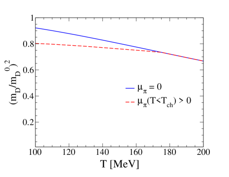
FIG. 2.: VDM resummation correction to $\Delta Q^{2}$ represented by the ratio of the squared electromagnetic Debye mass that includes effects of resummed $\rho\pi\pi$ loops (according to Eq. (34)) to that from the lowest-order result in strong interactions.

2 Chiral Reduction Scheme

The framework of Ref. [24] allows chiral master formulae to be used to relate $W_{\mu\nu}$ to experimentally extractable spectral functions in a model independent way. Using the analytical properties of ${W}_{00}$ in the complex $\omega$-plane, it follows that, in thermal equilibrium,

$${W}_{00}^{ab}(\omega,q) = -\frac{2\,{\rm Im}\,\Pi_{00}^{F,ab}(\omega,q)}{{\rm e}^{\beta|\omega|}+1}$$ (35)

$$= -\frac{2\,{\rm Im}\,\Pi_{00}^{R,ab}(\omega,q)}{{\rm e}^{\beta\omega}-1}\ ,$$ (36)

where the superscript $F$ ($R$) explicitly indicates the Feynman (retarded) charge-charge correlator. In this scheme, the vacuum part ${\Pi}^{0F}$ is common to a hadronic or partonic gas and is related to experimentally measured spectral functions. One has

$${\Pi}_{00}^{0F,ab}(M^{2})=i\int\,d^{4}x\,e^{iq\cdot x}\,\langle 0|T^{*}\,{{\cal V}}_{0}^{a}(x)\,\,{{\cal V}}_{0}^{b}(0)|0\rangle_{c}\,,$$ (37)

which is given by the longitudinal part of the isovector correlation function,

$$i\,\delta^{ab}\,(g_{00}\,M^{2}-q_{0}^{2})\,\Pi_{V}^{L}(M^{2})\,\,.$$ (38)

In a hadronic gas, the corrections to the leading spectral density follow from a virial expansion. Specifically,

$${\Pi}_{00}^{1F,ab}(\omega,q)=\sum_{A}\int\frac{d^{3}k}{(2\pi)^{3}}\,\frac{f^{\pi}(\omega_{k})}{2\omega_{k}}\,$$ (39)

$$\times i\int\,d^{4}x\,e^{iq\cdot x}\,\langle\pi(k)|T^{*}\,{{\cal V}}_{0}^{a}(x)\,\,{{\cal V}}_{0}^{b}(0)|\pi(k)\rangle_{c}$$ (40)

$$+...\,,$$ (41)

where $\omega_{k}^{2}=m_{\pi}^{2}+{\vec{k}}^{2}$. The ellipsis refer to corrections of higher order in pion- and nucleon-densities. The reduction of the forward Compton amplitude in Eq. (41) involves both the vector and axial-vector correlation functions. One finds

$${\rm Im}\,{\Pi}_{00}^{1F,ab}(\omega,q)\approx\delta^{ab}\,\int\frac{d^{3}k}{(2\pi)^{3}}\,\frac{f^{\pi}(\omega_{k})}{2f_{\pi}^{2}\,\omega_{k}}\,$$ (42)

$$\times\bigg{[}-4\vec{q}^{~{}2}\,{\rm Im}\,{\Pi}_{V}(q)$$ (43)

$$\qquad+2(\vec{k}+\vec{q})^{2}\,{\rm Im}\,{\Pi}_{A}(k+q)+(q\rightarrow-q)$$ (44)

$$\qquad+4(2\omega_{k}+\omega)\,(\omega_{k}\vec{q}^{~{}2}-\omega\,\vec{k}\cdot\vec{q})\,$$ (45)

$$\qquad\times{\rm Im}\,{\Pi}_{V}(q)\,{\rm Re}\,(\Delta_{R}(k+q)+q\rightarrow-q)\bigg{]}\,,$$ (46)

where $f_{\pi}$ is the pion decay constant and $\Delta_{R}(k)$ is the retarded pion propagator. In obtaining this result, only the dominant contributions to the Compton amplitude were retained. We note that the current algebra result follows from setting $k=0$, as a result of which the quantity in brackets in Eq. (46) takes the form

$$4\vec{q}^{~{}2}\,\left({\rm Im}\,{\Pi}_{A}(q)-\,{\rm Im}\,{\Pi}_{V}(q)\right)\,\,.$$ (47)

This relation illustrates the role of chiral symmetry restoration at next-to-leading order in the hadronic (pionic) density. Higher order corrections, not discussed here, are calculable in a similar way and in close analogy with calculations of photon and dilepton emissivities.

III CONNECTIONS TO HEAVY-ION EXPERIMENTS

Since fluctuations at the dilute freeze-out stage of a heavy-ion collision have been amply discussed in the literature, we focus here on how one might gain knowledge about fluctuations during the dense stages of the collision. Direct photons and dileptons, due to their negligible final state interaction in a heavy-ion collision, have long been recognized as sensitive probes of the physical state of strongly interacting matter. We are thus led to the following natural question: To the extent that electromagnetic observables at the CERN-SPS have been adequately described through a combination of hadronic and partonic approaches [25, 26, 28] (see [21] for a review), what are the implications of dilepton and photon spectra to be measured at RHIC and LHC on charge fluctuations of hadrons and partons during the dense stages of evolution? The answer to this question hinges critically on the outcome of upcoming measurements and on the ability of theory to model the complex evolution of the system created in a heavy-ion collision. In the following section, we provide a suitable theoretical framework that can be systematically improved.

A Longitudinally Expanding System in Local Thermal Equilibrium

In a heavy-ion collision, isospin fluctuations occur in an expanding environment that initially consists of partons which hadronize towards the end of evolution. In the Bjorken expansion scenario with boost invariance [29], the isospin charge per unit pseudo-rapidity can be schematically defined as $dQ^{a}/d\eta$. Boost invariance and charge conservation imply that

$$\frac{d(dQ^{a}/d\eta)}{d\tau}=0\,.$$ (48)

This conservation law assures that the mean fraction of isospin is the same in all frames, and constant throughout the proper time evolution. If this were to hold for the variance, then we would naively conclude that the rest frame results developed in the preceding section will trivially extend to the rapidity-binned fluctuations in a heavy-ion collision. Closer inspection reveals that this is not the case, as will be shown below.

Consider the thermal fluctuations in an expanding fluid-element that is characterized by its pseudo-rapidity $\eta=\tanh^{-1}\,(t/z)$ and proper time $\tau=\sqrt{t^{2}-z^{2}}$. Following the standard generalization of a conserved current to a moving frame, we define the isospin charge operator

$${\cal Q}_{\Delta}^{a}(\tau,\eta)=\int d\sigma^{\mu}\ {\cal V}_{\mu}^{a}$$ (49)

in a fixed pseudo-rapidity interval of extent $\Delta$ centered around $\eta$. Above, $\sigma^{\mu}$ represents a 3-dimensional hyper-surface in space-time which is orthogonal to the local fluid 4-velocity $u^{\mu}=\gamma(1,\vec{\beta})$. From here on, we restrict ourselves to purely longitudinal expansion for the sake of simplicity. With $d\sigma^{\mu}=dx_{\perp}(dz,0_{\perp},dt)$, the charge becomes

$${\cal Q}_{\Delta}^{a}(\tau,\eta)=\int dx_{\perp}\int\limits_{\eta_{-}}^{\eta_{+}}\tau d{\underline{\eta}}\ u_{\|}^{\mu}\,{\cal V}^{a}_{\mu}\left(\tau{\rm ch}{\underline{\eta}},x_{\perp},\tau{\rm sh}{\underline{\eta}}\right)\,,$$ (50)

where $\eta_{\pm}=\eta\pm\Delta/2$. The quantity $u_{\|}^{\mu}=({\rm ch}{\underline{\eta}},0_{\perp},{\rm sh}{\underline{\eta}})$ is equivalent to the longitudinal Lorentz boost operator $\Lambda_{0}^{~{}\mu}$, as it should. The binned isospin fluctuations can then be expressed as

$$\langle{\cal Q}_{\Delta}^{a}(\tau,\eta)\ {\cal Q}_{\Delta}^{b}(\tau,\eta)\rangle_{c}=\int dx_{\perp}\ dx^{\prime}_{\perp}\int\limits_{\eta_{-}}^{\eta_{+}}\int\limits_{\eta_{-}}^{\eta_{+}}\tau d\underline{\eta}\ \tau d\underline{\eta}^{\prime}$$ (51)

$$\times\ u_{||}^{\mu}\ {u^{\prime}}_{||}^{\nu}\ \langle{\cal V}_{\mu}^{a}(x_{||},x_{\perp})\,{\cal V}_{\nu}^{b}(x_{||}^{\prime},x_{\perp}^{\prime})\rangle_{c}\,,$$ (52)

where $x_{\|}\equiv\tau({\rm ch}{\underline{\eta}},{\rm sh}{\underline{\eta}})$. The averaging is carried in a hadronic or a partonic gas in equilibrium at temperature $T(\tau)=1/\beta(\tau)$ and pertinent chemical potentials. (We will return to discuss some specific issues related to non-equilibrium situations in Sec. IV.) Using translational invariance in the transverse direction along with a Fourier transform of the unordered charge correlator,

$${\bf W}_{00}^{ab}(\omega,q)=\int d^{4}x\ {\rm e}^{iq\cdot x}\ \langle{\cal V}_{0}^{a}(x)~{}{\cal V}_{0}^{b}(0)\rangle\ ,$$ (53)

Equation (52) can be cast in the form

$$\langle Q^{a}_{\Delta}(\tau,\eta)\,\,Q_{\Delta}^{b}(\tau,\eta)\rangle_{c}={V_{\perp}}\int\frac{d\bar{\omega}\,d\bar{q}_{z}}{(2\pi)^{2}}\qquad\qquad$$ (54)

$$\times\ W_{L}^{ab}(\bar{\omega}/\tau,0_{\perp},\bar{q}_{z}/\tau)\ \frac{|F_{\Delta}(\eta,;\bar{\omega},\bar{q}_{z})|^{2}}{\bar{\omega}^{2}-\bar{q}_{z}^{2}}\ .$$ (55)

Here, we have introduced dimensionless variables $\bar{\omega}=\tau\omega$ and $\bar{q}=\tau q$ and exploited the relations

$$W_{00}=\frac{q^{2}}{M^{2}}W_{L}\,,~{}W_{0z}=\frac{\omega q_{z}}{M^{2}}W_{L}\,,~{}{\rm and}~{}W_{zz}=\frac{\omega^{2}}{M^{2}}W_{L}\,,$$ (56)

as required by current conservation. The kinematical “formfactors” in Eq. (55) arise from restricting the isospin charge to a bin of width $\Delta$ in pseudo-rapidity and are given by

$$F_{\Delta}\ F_{\Delta}^{*}=\left[2~{}\sin\left({\rm sh}\left(\frac{\Delta}{2}\right)\ [\bar{\omega}\,{\rm sh}\eta-\bar{q}_{z}\,{\rm ch}\eta]\right)\right]^{2}\ .$$ (57)

The occurrence of solely the longitudinal part $W_{L}$ is a consequence of the underlying assumption of purely longitudinal fluid flow and current conservation. The presence of transverse flow would naturally involve the transverse part $W_{T}$ as well.

We recall that for dilepton emission, the combination $2~{}W_{T}+W_{L}$ contributes, whereas in photon emission only $W_{T}$ is needed. At large proper time $\tau$, the correlation function is probed around $\omega\approx q\approx 0$. In general, the fluctuations in pseudorapidity bins represented by Eq. (55) are sensitive to both space-like and time-like physics. As noted in the previous section, the space-like contribution is driven by screening and Landau damping, while time-like physics governs decays or production. The latter are at the origin of photon and dilepton emissivities. To lowest order in temperature, the imaginary part of the relevant polarization is empirically accessible through $e^{+}e^{-}$ annihilation for $M^{2}>0$. Since thermal fluctuations preserve isospin, the integrand in Eq. (55) (modulo $F$) is a consequence of the fluctuation dissipation theorem (cf. Eq. (36)).

Employing boost invariance, we can focus on a window of width $\Delta$ centered around mid-rapidity $\eta=0$. Inserting Eq. (36) into Eq. (52), we obtain (omitting isospin indices)

$$\frac{\langle{\cal Q}_{\Delta}^{2}(\tau)\rangle}{V_{\perp}}=(-2)\,\left[2\,{\rm sh}(\Delta/2)\right]^{2}\int\frac{d\bar{\omega}\,d\bar{q}}{(2\pi)^{2}}\qquad\quad$$ (58)

$$\qquad\times\ \frac{{\rm Im}W_{R}^{00}(\bar{\omega}/\tau,0_{\perp},\bar{q}/\tau)}{{\rm e}^{\beta\,\bar{\omega}/\tau}-1}\ \left(\frac{\sin\left[\bar{q}\,{\rm sh}(\Delta/2)\right]}{\bar{q}\,{\rm sh}(\Delta/2)}\right)^{2}\ .$$ (59)

This relation is one of the principal results of this work. It explicitly demonstrates that fluctuations are sensitive not only to screening, but also to emissivities. Such a feature is in contrast to the case of the rest-frame fluctuations discussed in Sec. II, and stems from the general properties of boost transformations of charge-charge correlators.

Equation (59) also shows that fluctuations are proportional to the “size” of the pseudorapidity interval through ${\rm sh}^{2}(\Delta/2)$, vanishing for $\Delta=0$ as they should. The dominant contribution arises from long wavelengths $\lambda\simeq 2\pi/q\geq 2\pi\,\tau\,{\rm sh}(\Delta/2)$ for which ${\rm sin}^{2}x/x^{2}\approx 1$, and small frequencies $f=\bar{\omega}/2\pi\tau\simeq 1/2\pi\tau_{F}$, where $\tau_{F}$ is a typical lifetime of the expanding system. The limitation on frequency is enforced by the requirement that for large times, one has to recover the equilibrium screening limit that was discussed in the previous section. That this is indeed the case can be seen as follows: For large $\tau$, the oscillating factor on the right-hand-side of Eq. (59) collapses the $\bar{q}$ integration to its saddle point at $\bar{q}\simeq 0$. Furthermore, the denominator becomes ${\rm e}^{\beta\,\bar{\omega}/\tau}-1\simeq\beta\bar{\omega}/\tau$. Using this, one recovers the dispersion relation, Eq. (29), for the Debye mass. Note also that the factor $z=2\tau\,{\rm sh}(\Delta/2)$ combines with $V_{\perp}$ to yield the spatial 3-volume $V_{3}$.

Figure 3 displays results of the quantity $R=\langle{\cal Q}_{\Delta}^{2}(\tau)\rangle/V_{3}s(\tau)$ from numerical evaluations of Eq. (59) and Eq. (13) for a model system comprised of an ideal QGP ($N_{f}=2$) in the partonic phase and massless pions in the hadronic phase. The time evolution of temperature has been taken to result from a boost-invariant longitudinal expansion [29] in which

$$T(\tau)=\left\{\begin{array}[]{ll}T_{0}~{}(\tau_{0}/\tau)^{1/3}&,~{}~{}~{}~{}\tau_{0}<\tau<\tau_{1}\quad({\rm QGP})\\ T_{c}&,~{}~{}~{}~{}\tau_{1}<\tau<\tau_{2}\quad({\rm Mixed})\\ T_{c}~{}(\tau_{2}/\tau)^{1/3}&,~{}~{}~{}~{}\tau_{2}<\tau\qquad\quad\ ({\rm HG})\ .\end{array}\right.\,$$ (63)

The numerical values of the time constants, $\tau_{0}=1$ fm/c, $\tau_{1}=2$ fm/c, $\tau_{2}=5$ fm/c and the critical temperature, $T_{c}=170$ MeV, were chosen to generate conditions that resemble those at SPS energies (e.g., $T_{0}=T_{c}(\tau_{1}/\tau_{0})^{1/3}\simeq 214$ MeV). In the mixed phase, the fluctuation content $R=fR_{QGP}+(1-f)R_{\pi}$ is a weighted sum with the appropriate volume fractions $f$ and $(1-f)$ of the QGP and hadronic phases, respectively.

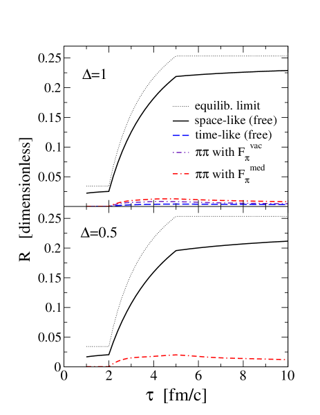
FIG. 3.: Proper-time evolution of charge fluctuations per unit 3-volume, Eq. (59), normalized to the appropriate entropy density, Eq. (13), for an ideal QGP ($\tau\leq 2$ fm/c) and a massless pion gas ($\tau\geq 5$ fm/c) in a locally thermalized, longitudinally expanding fluid. The upper (lower) panel shows results for a pseudorapidity window of size $\Delta=1$ (0.5). The solid (long-dashed) curves correspond to contributions from the space-like (time-like) part of the charge-charge correlator. The dash-dotted and double-dash-dotted lines are results for the time-like hadronic contribution wherein $\pi\pi$ correlations have been included through the free pion-e.m. formfactor $F_{\pi}^{vac}(M^{2})$ and an in-medium $F_{\pi}^{med}(M^{2})$ (with twice larger $\rho$-width), respectively. The dotted lines indicate the static equilibrium limit, $Tm_{D}^{2}/s$.

In the non-interacting case (employing for Im $W^{00}_{R}$ Eqs. (24) and (27) generalized to finite $q$), fluctuations are clearly dominated by the space-like contribution of the correlator (solid curves in Fig. 3), especially at small proper-times in the partonic phase. The latter fact is due to the fermionic character of the charge carriers (see Eq. (27)). However, as shown in Sec. II F, the inclusion of hadronic interactions tends to suppress the space-like contribution (not shown in the figure), but enhances the time-like one, as is evident from the dash-dotted and double-dash-dotted curves in the upper panel. This behavior becomes more pronounced if the size of the rapidity bin is reduced (see the lower panel of Fig. 3).

In general, $\Delta$ should be large enough to enhance the volume-to-surface effect, but small enough to avoid the constraint of overall charge conservation in the nuclear system.

We emphasize that the evolution of fluctuations shown in Fig. 3 refers to a highly idealized model, especially in the hadronic phase. As stressed in Sec. II C, the entropy density of a more realistic hadronic resonance gas will be several times larger than that of a massless pion gas [5], entailing a reduction in $R$. To illustrate its effect, we show in Fig. 4 the results of a calculation in which the pure hadronic phase begins with an entropy density $s\simeq 5~{}{\rm fm}^{-3}$, a value representative of a hadronic resonance gas at $T_{c}=170~{}\rm{MeV}$. Finite hadron masses also imply that $s_{HG}$ falls off faster than $T^{3}$ with decreasing temperature, which has been simulated by employing $s_{HG}(\tau)=s_{HG}(T_{c})~{}(\tau_{2}/\tau)^{1.35}$, indicated by thermal fireball calculations [25]. Consequently, the static limit of the ratio $R$ increases with falling temperature in the expanding resonance gas for $\tau>5$ fm/c (see the dotted lines in Fig. 4). To minimally account for the effect of additional states in the numerator of $R$ (this contains the magnitude of fluctuations), we have also included contributions from kaons to the hadronic e.m. correlator (in the massless limit). This amounts to a simple increase of $\langle{\cal Q}_{\Delta}^{2}(\tau)\rangle/V_{3}$ by a factor of 2 compared with the result for massless pions. The presence of massless strange quarks in the QGP hardly affects the equilibrium value of $R_{QGP}$, reducing it from 0.034 (for $N_{f}=2$) to 0.032 (for $N_{f}=3$). The relative role of space- and time-like contributions to $R$ does not change as compared to Fig. 3.

More realistic hadronic correlators, as were found necessary to explain the dilepton data from heavy-ion collisions at SPS energies, are characterized by a substantial reshaping of the pion e.m. form factor, in particular through an appreciable accumulation of strength at low invariant masses. We anticipate that the use of such correlators in Eq. (59) will enhance the role of the time-like region. Results for the simplified cases considered here are thus to be regarded as suggestive. They clearly indicate, however, that calculations of a more realistic evolution of $R$ employing improvements in (i) the equation of state, (ii) space-time evolution, and (iii) appropriate electromagnetic correlators are worthwhile. Developments in this regard are in progress and will be reported separately.

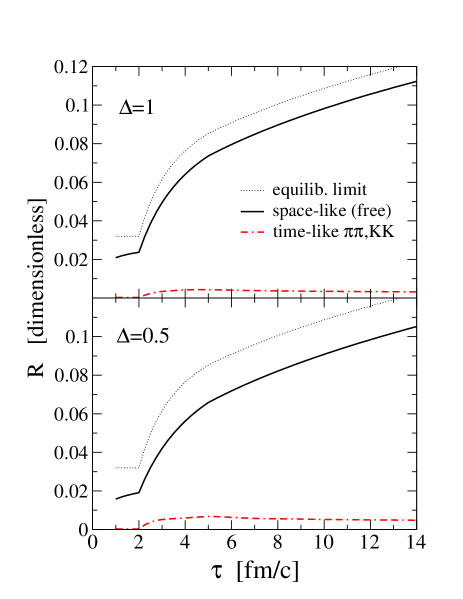
FIG. 4.: Same as Fig. 3 but with the following improvements: (i) In the hadronic phase, the entropy density has been calculated for a hadronic resonance gas, (ii) The e.m. correlator includes contributions from $K^{+}K^{-}$ states in addition to $\pi^{+}\pi^{-}$ states (both are calculated in the massless limit); and (iii) In the QGP, massless strange quarks have been included in both the entropy density and e.m. correlator.

B Relation to Other Works

Our main result from the previous section, Eq. (59), bears some resemblance to the results obtained in Ref. [8], in particular to Eq. (18) therein, which, in the notation of Ref. [8], reads

$$\langle(\Delta Q)^{2}\rangle = \int\frac{dk}{2\pi}\ \frac{\sin^{2}(k\Delta y/2)}{(k/2)^{2}}\ \chi_{k}$$ (65)

$$\quad\times[1-\exp\{-k^{2}(\Delta y_{\rm diff})^{2}\}]\ .$$

This relation describes the relaxation of the moments of charge fluctuations in one-dimensional rapidity space through the purely space-like density-density correlation function $\chi_{k}$ and the mean diffusion, $\Delta y_{\rm diff}$, of a particle during time $\tau$. The $(\sin x/x)^{2}$ factor above is equivalent to a similar factor in Eq. (59) and arises as a consequence of boost invariant longitudinal expansion without transverse flow. The time-dependent exponential factor in Eq. (65) results from non-equilibrium effects, which were treated using a Gaussian solution of a Fokker-Planck equation [8]. Non-equilibrium effects are not accounted for in Eq. (59) (see, however, our discussion of such effects in the following section). Our derivation of Eq. (59), on the other hand, includes the full 4-dimensionally transverse structure of the conserved isospin current operator, evaluated within a locally equilibrated relativistic fluid. This induces additional quantum effects associated with the finite time scale of the expansion thereby involving the time-like region of the correlation function. These features are not captured by the treatment of Ref. [8], in arriving at Eq. (65).

It is worthwhile to point out that, during the dense stages of evolution in a heavy-ion collision, the assumption of local thermal equilibrium among the constituents of matter has been gainfully employed to understand photon and dilepton emission. Calculations in the CERN SPS regime have shown that a fair agreement exists between theory and experiment [25, 26, 28]. In the context of charge fluctuations the equilibrium assumption is supported by the estimates of $\Delta y_{\rm diff}$ presented in Ref. [5], and also by the more quantitative analysis of Ref. [8], where the diffusion equation (65) was solved with inputs from microscopic transport calculations [8]. It was shown there that, due to frequent rescattering in the hadronic phase of a heavy-ion collision, the diffusion of charge in rapidity space is effective in keeping fluctuations close to its equilibrium value (within $\sim$ 20%) until freeze-out at both SPS and RHIC [8]. This is consistent with preliminary experimental data, which point to a dilute hadron gas in the vicinity of thermal freeze-out.

Notwithstanding these observations, we study in the following section a somewhat different source of non-equilibrium effects, namely, fluctuations in the temperature. This was suggested some years ago as a means of extracting the heat capacity of the hadronic gas close to freeze-out [11]. Here we explore connections between temperature and charge fluctuations, and examine the consequences of the presence of non-equilibrium effects in heavy-ion collisions.

IV DEVIATIONS FROM LOCAL THERMAL EQUILIBRIUM

Non-thermal fluctuations are generally caused by complex microscopic and dissipative phenomena. A microscopic or QCD-based description of such phenomena is beyond the scope of this paper. Instead, we use a macroscopic approach that is based on a stochastic or maximum noise assumption. We adduce arguments to show that a non-thermal or early-stage isospin fluctuation can survive the expansion only if it is accompanied by a large temperature fluctuation at freeze-out. Since temperature fluctuations reflect the heat capacity of the underlying phase, we consider two different possibilities by treating non-equilibrium effects stochastically through additive (Gaussian) or multiplicative (power-law) heat flow.

A Gaussian Fluctuations

Let $T(\tau)$ be the temperature at a given proper time $\tau$, and $T_{*}=1/\beta_{*}$ the equilibrium (mean) temperature. Let $T(\tau)$ relax stochastically due to heat flow. In a phase in which the heat capacity $C$ depends strongly on $T_{*}$, thermodynamics implies that the variance of the temperature distribution is bounded. The stochastic evolution is “Brownian”, and the relaxation of $T(\tau)$ is governed through additive white noise. The corresponding Langevin equation is of the form

$$\frac{dT}{d\tau}+\frac{1}{\tau_{*}}\,\left(T(\tau)-\xi(\tau)-T_{*}\right)=0\,\,,$$ (66)

where $\tau_{*}$ is the temperature relaxation time, and $\xi(\tau)$ is a white noise, i.e., uncorrelated in time and with zero mean. In this case,

$$\langle\langle\xi(\tau)\,\xi(\tau^{\prime})\rangle\rangle=2D\,\delta(\tau-\tau^{\prime})\,\,.$$ (67)

The average in Eq. (67) is performed over stochastic noise distributions $\xi$, the strength of which is characterized by the variance $D$. The distribution of temperatures ${\bf P}(\tau,T)$ associated with the additive Langevin equation (66) obeys a Fokker-Planck equation [30]. Specifically,

$$\frac{\partial{\bf P}}{\partial\tau}(\tau,T)= -\frac{\partial}{\partial T}\left(\frac{(T_{*}-T)}{\tau_{*}}\,\,{\bf P}(\tau,T)\right)$$ (69)

$$+\frac{1}{2}\,\frac{\partial^{2}}{\partial T^{2}}\,\left(\frac{2D}{\tau_{*}^{2}}\,\,{\bf P}(\tau,T)\right)$$

with a drift rate $\nu_{T}=(T_{*}-T)/\tau_{*}$ and a constant diffusion rate $\nu_{\rm diff}=2D/{\tau_{*}^{2}}$. The general solution is an evolving Gaussian

$${\bf P}(\tau,T)=\sqrt{\frac{1}{2\pi\,\sigma^{2}(\tau)}}\ {\rm e}^{-(T-\langle T(\tau)\rangle)^{2}/2\sigma^{2}(\tau)}\,\,$$ (70)

with a stochastic mean

$$\langle T(\tau)-T_{*}\rangle=(T(0)-T_{*})\ {\rm e}^{-\tau/\tau_{*}}\,.$$ (71)

Above, single angular brackets denote an average with respect to the temperature distribution. The variance is given by

$$\sigma^{2}(\tau)=\frac{D}{\tau_{*}}+\left(\sigma^{2}(0)-\frac{D}{\tau_{*}}\right)\,{\rm e}^{-2\tau/\tau_{*}}\ ,$$ (72)

which reduces to $\sigma^{2}(\tau\to\infty)=D/\tau_{*}$ in the stationary case, reflecting the thermodynamic limit. It can thus be related to the heat capacity, $C=T_{*}^{2}/\sigma^{2}$, which depends strongly on $T_{*}$. The stationary temperature distribution takes the form

$${\bf P}_{S}(T)={\bf P}(\infty,T)=\sqrt{\frac{C}{2\pi\,T^{2}_{*}}}\ {\rm e}^{-C(T-T_{*})^{2}/2T_{*}^{2}}\ .$$ (73)

The standard Gaussian nature of the fluctuations attests to the additive character of white noise. Obviously, a large heat capacity strongly limits the character of fluctuations through exponentially small tails in the stationary distribution, Eq. (73).

B Power-Law Fluctuations

Here we explore the consequences of a more speculative scenario, that is, a phase in which the heat capacity $C$ is nearly constant so that the equilibrium variance grows with the mean temperature squared, $\sigma^{2}=T^{2}_{*}/{C}$. Such a behavior can be constructed by starting from a Langevin equation in which the noise is introduced multiplicatively using the Ito-prescription [31]. In our case, this is realized by setting

$$\frac{dT}{d\tau}+\frac{1}{\tau_{*}}\,\left[(1+\xi(\tau))\,T(\tau)-T_{*}\right]=0\ ,$$ (74)

where, as before, $\xi(\tau)$ is a white noise with zero mean and variance $2D$. Arguments similar to the ones used in the previous section yield a Fokker-Planck equation analogous to Eq. (69) with the same drift rate, $\nu_{T}=(T_{*}-T)/\tau_{*}$, but a non-constant diffusion rate, $\nu_{\rm diff}=2DT^{2}/{\tau_{*}}^{2}$, which is the key difference from the result in Eq. (66). In the steady state, the distribution of temperatures is now given by

$${\bf P}_{S}(T)=\frac{(1+C)^{1+C}}{\Gamma(1+C)}\,\left(\frac{T_{*}}{T}\right)^{3+C}\,\,\frac{{\rm e}^{-(1+C)\,T_{*}/T}}{T_{*}}\,,$$ (75)

where the corresponding variance, $\sigma^{2}=T_{*}^{2}/(\tau_{*}/D-1)$, allows us to replace $\tau_{*}/D$ by $1+C$. Note that this is the desired behavior for a constant heat capacity. Larger temperatures are only power-law suppressed as a direct consequence of the multiplicative character of the noise. If we further assume that the temperature relaxation time $\tau_{*}$ is small in comparison to the underlying flow time in the evolution, we may average the temperature fluctuations around the instantaneous mean $T_{*}=1/\beta_{*}$ using Eq. (75). For the leading temperature contribution to the electromagnetic correlator, e.g., Eq. (41), this amounts to

$$\left\langle f^{B}(\omega;T)\right\rangle = \left\langle\frac{1}{{\rm e}^{\omega/T}-1}\right\rangle$$ (76)

$$= \sum_{n=1}^{\infty}\left(\frac{1}{1+n\,\frac{\omega}{T_{*}\,(1+C)}}\right)^{(2+C)}\ .$$ (77)

Again, we see that temperature fluctuations turn the exponential suppression of high energies (implicit in equilibrium Bose and Fermi distribution functions) into a power-law suppression. The larger the heat capacity $C$ of the phase considered, be it hadronic or some sort of mixed phase, the stronger will be the power-law suppression, and hence the closer the temperature distribution to a Gaussian, as expected. These results can be readily adapted to a dynamical description, e.g., a hydrodynamical simulation, which will be reported in future work.

V SUMMARY AND OUTLOOK

Our purpose in this paper has been to highlight the interdependence of fluctuations in isospin charge and electromagnetic emissivities in the strongly interacting matter encountered during the dense stages of a heavy-ion collision. We have established such connections both in an infinite system at rest, as well as in a relativistically expanding fluid to mimic some of the dynamics present in high-energy nuclear collisions.

In the static case, we have emphasized that well-known relations between the fluctuations of the charged constituents of matter and its electric screening mass imply an intimate connection to the emission of dileptons/photons. Both of these can be calculated from the retarded current-current correlation function, or the photon self-energy, in hot and dense partonic or hadronic matter. Consequently, analyses of dilepton and photon observables that are based on the e.m. correlation function can be systematically applied to study medium effects on fluctuations during the dense stages of a heavy-ion collision. Two hadronic approaches were used to exemplify that close to the expected phase boundary, hot and dense hadronic matter might exhibit fluctuations of similar magnitude as an equilibrated partonic medium (QGP). Clearly, further work is required to improve these estimates.

In the case of an expanding fluid, we derived an expression for the fluctuations in a locally equilibrated fluid element as a function of proper time and over a finite range in pseudo-rapidity. Isospin conservation, which governs the 4-dimensionally transverse Lorentz-structure of the correlation function, implies that fluctuations depend on both transverse and longitudinal components. Furthermore, the finite time scale $\sim~{}\tau_{fo}$ dictated by the strong interaction dynamics in a nuclear collision implies that both space-like and time-like processes are involved. At a given freeze-out proper time $\tau_{fo}$ and within a rapidity window of width $\Delta$, the thermal isospin fluctuations are dominated by constituents with typical frequencies $f\approx 2\pi/\tau_{fo}$ and wavelengths $\lambda\approx\pi\tau_{fo}\,{\rm sh}(\Delta/2)$.

Our analysis of non-equilibrium effects associated with possible temperature fluctuations indicates that a large isospin fluctuation at the early partonic stage can survive the course of a relativistic heavy-ion collision only if a large temperature fluctuation occurs simultaneously at freeze-out in the same event. Given a large and strongly temperature-dependent heat capacity of a hadronic gas, this scenario seems unlikely.

Prospects for the future include: (1) A determination of the Debye mass of the system at the dilute freeze-out stage of a heavy-ion collision; this could be accomplished solely through measured results of particle multiplicities and particle correlations using Hanbury-Brown and Twiss analyses. An intriguing question in this connection is whether or not the Debye mass at freeze-out remains constant from AGS through LHC energies; and (2) A delineation of the role of charge fluctuations during the dense stages of the collision through a study of electromagnetic emissivities; this is a more challenging task inasmuch as an understanding of the measured dilepton and photon yields will necessarily require a detailed theoretical analysis to unravel the phase structure of the rapidly evolving produced matter.

Our ongoing investigations include a dynamical simulation of the collision, in which the effects of strong interactions are studied through the equation of state and the effects of fluctuations in dense matter are studied through its electromagnetic radiation.

REFERENCES

- [1] M. Roland et al., (NA49 collaboration), Nucl. Phys. A638, 91c, (1998); H. Appelshäuser et al., (NA49 collaboration), Phys. Lett. B459 679 (1999); J.G. Reid, (NA49 collaboration), Nucl. Phys. A661 407c (1999); K. Perl, NA49 note 244.
- [2] L. McLerran, Phys. Rev. D36, 3291 (1987).
- [3] L. van Hove, Z. Phys. C21, 93 (1984); M. Gyulassy et al., Nucl. Phys. B237, 477 (1984); A. Bialas and R. Peshanski, Nucl. Phys. B273, 703 (1986).
- [4] H. Heiselberg, Phys. Rep. 351, 161 (2001).
- [5] M. Asakawa, U. Heinz and B. Müller, Phys. Rev. Lett. 85, 2072 (2000).
- [6] S. Jeon and V. Koch, Phys. Rev. Lett. 85, 2076 (2000).
- [7] K. Fialkowski and R. Wit, hep-ph/0006023.
- [8] E.V. Shuryak and M.A. Stephanov, Phys. Rev. C63, 064903 (2001).
- [9] G.F. Bertsch, Phys. Rev. Lett. 72, 2349 (1994).
- [10] D. Ferenc, U. Heinz, B. Tomasik, U.A. Wiedemann and J. G. Cramer, Phys. Lett. B457, 347 (1999).
-
[11]
L. Stodolsky, Phys. Rev. Lett. 75, 1044 (1995);
E. Shuryak, Phys. Lett. B423, 9 (1998). - [12] L.D. Landau and E.M. Lifshitz, Statisticsl Physics, 3. edition, Pergamon Press 1980.
- [13] S. Doniach and E.H. Sondheimer, Green’s Functions for Solid State Physicists (London: Imperial College Press; River Edge NJ: Distributed by World Scientific Pub., c1998).
- [14] J. Kapusta, Finite Temperature Field Theory, Cambridge University Press 1989.
- [15] M. Prakash and I. Zahed, Phys. Rev. Lett. 69, 3282 (1992).
- [16] J.-P. Blaizot, E. Iancu, and R.R. Parwani, Phys. Rev. D52, 2543 (1995).
- [17] R. Venugopalan and M. Prakash, Nucl. Phys. A546, 718 (1992).
- [18] M. Le Bellac, Thermal Field Theory, Cambridge University Press 1996.
- [19] S. Gottlieb et al., Phys. Rev. D55 (1997), 6852.
- [20] V.L. Eletsky, J.I. Kapusta, and R. Venugopalan, Phys. Rev. D48, 4398 (1993).
- [21] R. Rapp and J. Wambach, Adv. Nucl. Phys. 25, 1 (2000).
- [22] C. Gale and J. Kapusta, Nucl. Phys. B357, 65 (1991).
- [23] R. Rapp, G. Chanfray and J. Wambach, Nucl. Phys. A617, 472 (1997).
- [24] J. Steele, H. Yamagishi and I. Zahed, Phys. Rev. D56, 5605 (1997).
- [25] R. Rapp and J. Wambach, Eur. Phys. J. A6, 415 (1999).
- [26] J. Steele and I. Zahed, Phys. Rev. D60, 037502 (1999).
- [27] S. Gao and C. Gale, Phys. Rev. C57, 254 (1998).
- [28] P. Huovinen and M. Prakash, Nucl. Phys. A661, 522 (1999).
- [29] J.D. Bjorken, Phys. Rev. D27, 140 (1983).
- [30] H. Risken, The Fokker-Planck Equation, Springer-Verlag 1989.
-
[31]
L. Borland, Phys. Lett. A245, 67 (1998);
G. Wilk and Z. Wlodarczyk, hep-ph/9908459.