Fine Structure of Oscillons in the
Spherically Symmetric $\phi^{4}$ Klein-Gordon Model

Abstract

We present results from a study of the fine structure of oscillon dynamics in the 3+1 spherically symmetric Klein-Gordon model with a symmetric double-well potential. We show that in addition to the previously understood longevity of oscillons, there exists a resonant (and critical) behavior which exhibits a time-scaling law. The mode structure of the critical solutions is examined, and we also show that the upper-bound to oscillon formation (in $r_{0}$ space) is either non-existent or higher than previously believed. Our results are generated using a novel technique for implementing non-reflecting boundary conditions in the finite difference solution of wave equations. The method uses a coordinate transformation which blue-shifts and “freezes” outgoing radiation. The frozen radiation is then annihilated via dissipation explicitly added to the finite-difference scheme, with very little reflection into the interior of the computational domain.

I Introduction

There is a long history in physics and mathematics of trying to find new non-trivial solutions to nonlinear wave equations. The literature on the subject goes back at least as far as 1845 when J. Scott Russell published a paper about a surface wave he witnessed travel for almost two miles in a shallow water channel (the first scientifically reported soliton)Russell . Since then there has been much effort directed towards understanding stable localized solutions to nonlinear wave equations: the classical kink-soliton, topological defects (monopoles, cosmic strings, and domain walls)Vilenkin , and nontopological defects (such as Q-balls)Friedberg ; Coleman , are but a few examples. However, localized but unstable solutions have been discussed much less frequently and in this paper we focus our attention on one such solution, the oscillon.

The definition of oscillon varies slightly depending on context, but here we refer to localized, time-dependent, unstable, spherically symmetric solutions to the nonlinear Klein-Gordon equation. Although oscillons are unstable, their lifetimes are long compared to a dynamical time. Oscillons were originally discovered by Bogolubsky and Makhan’kov BogMak1 ; BogMak2 (who called them “pulsons”), and were later studied in more detail by Gleiser gleiser0 and by Copeland et al gleiser1 .

Oscillons can be formed via the collapse of field configurations (initial data) that interpolate between two vacuum states ($\phi_{+}$ and $\phi_{-}$) of a symmetric double well potential (SDWP). In spherical symmetry, such a configuration is a bubble, where the interpolating region is the bubble “wall” that separates the two vacuum states at some characteristic radius (where in this work we always use $\phi_{-}$ as the large-$r$ vacuum state). An oscillon formed this way typically has three distinct stages in its evolution. First, immediately following the bubble collapse a large percentage of its energy is radiated away. As will be discussed below, this can happen either through localized field oscillations, or through bounces reminiscent of the 1+1 dimensional kink-antikink, ($K{\bar{K}}$), scattering 1dkak_campbell . After the initial radiative phase, the solution settles into the oscillon stage. Here the field is localized with a shape roughly that of an origin-centered gaussian, with the field value asymptotically approaching the large-$r$ vacuum state. Due to the asymmetry of the potential about either minimum, the field oscillates about $\phi_{-}$ (the large-$r$ vacuum) such that the time-averaged value of the field lies between the two vacua, ie. $\phi_{-}<\langle\phi\rangle<\phi_{+}$ where $\langle\,\cdots\,\rangle\equiv T^{-1}\int_{0}^{T}\,\cdots\,dt$ as in gleiser1 . For typical initial field configurations the energy of the oscillon is slowly radiated away, approaching a specific “plateau” value. In the third and final stage of evolution, the oscillon stops oscillating and disperses, radiating away its remaining energy.

Much of the original excitement about oscillons arose from the fact that their long lifetimes could potentially alter the dynamics of a cosmological phase transition. However, since oscillons are unstable, their ability to affect such a phase transition depends crucially on their lifetimes. Previous studies by Copeland et al gleiser1 , used dynamical grid methods to study oscillon dynamics and treated the initial radius, $r_{0}$, of the bubble (shell of radiation), as a free parameter. These studies showed not only that oscillon lifetimes can be comparable to the age of the universe (at the GUT scale), but that oscillons are formed from a wide range of initial bubble radii. However, the computational demands of the dynamical grid methods employed in gleiser1 prevented a detailed study of the $r_{0}$ parameter space.

A key problem in the accurate, long-time simulation of oscillons is the treatment of boundary conditions at the outer edge, $r=r_{\rm max}$, of the computational domain. It is standard practice in the computational solution of nonlinear field equations to use finite difference techniques applied to functions defined on a lattice of gridpoints. If a static, finite-sized domain is used; i.e. if $r_{\rm max}$ is fixed, then one needs to employ a method which minimizes the amount of radiation (energy) which is artificially reflected at $r=r_{\rm max}$. With massless scalar fields, and in spherical symmetry, this can be done quite easily simply by imposing a discrete version of an “outgoing radiation”, or Sommerfeld, condition. However, for the case of massive scalar fields, or more generally, for fields with non-trivial dispersion relations, the Sommerfeld condition is only approximate, and its use generically results in significant reflection at $r=r_{\rm max}$, and subsequent contamination of the interior solution.

A surefire fix for the outer-boundary problem is to use a dynamically growing grid (as in gleiser1 ), so that $r_{\rm max}=r_{\rm max}(t)$, and lattice points are continuously added to extend the computational domain as needed. Alternatively, compactified coordinates, or coordinates which propagate outwards faster than any characteristic speed in the problem can be used, but in these cases, new gridpoints also need to be continuously added to the mesh in order to maintain adequate resolution of solution features. These methods are somewhat more efficient than the use of a static mesh with $r_{\rm max}$ chosen so that no signals reach the outer boundary during the integration period of interest, $T$. However, for long-lived solutions, the mesh soon becomes quite large, and the computation time tends to be proportional to $T^{2}$.

Recently, Gleiser and Sornborger newgleiser introduced an adiabatic damping method which adds an explicit damping term to the equations of motion, and which has been shown to absorb outgoing massive radiation extremely well in 1D (spherical) and 2D (cylindrical) simulations. Here we present an alternate approach for dealing with outgoing massive scalar fields which is quite general and quite different from previously used methods of which we are aware. The technique involves the use of a specially chosen coordinate system that “freezes” and blue-shifts outgoing radiation in a relatively thin layer located away from the central region where the dynamics of principal interest unfold. The addition of a standard type of finite-difference dissipation ko then “quenches” the blue-shifted, frozen radiation, and very little energy is reflected back into the interior region. This approach, like that described in newgleiser , has the advantage that a static and uniform finite-difference mesh can be used, so that computational time scales linearly with the integration period, $T$.

Our new technique was crucially important to our discovery and detailed study of fine structure in a well-known (and still much studied) nonlinear system. Specifically, we have found strong evidence for a family of resonant oscillon solutions in the SDWP model. Each of these solutions appears to possess a single unstable mode in perturbation theory, and by tuning the family parameter, $r_{0}$, in the vicinity of a specific resonance, we can tune away that mode, producing oscillons which live longer and longer as we tune closer and closer to the precise resonant value, $r_{0}^{\star}$. This leads to a view of oscillons as being analogous to the Type I critical solutions which have been discovered in the context of gravitational collapse TypeI , and as in that case, we find compelling evidence for power-law scaling of the oscillon lifetime, $\tau$:

$$\tau\,\sim\,c_{r}|r_{0}-r_{0}^{\star}|^{\gamma_{r}}$$ (1)

where $c_{r}$ is an overall scale factor set by the particular resonance, and $\gamma_{r}$ is a resonance-dependent exponent which is presumably the reciprocal Lyapounov exponent associated with the resonance’s single unstable mode.

In addition, contrary to previous claims gleiser1 ; newgleiser , we see no hard evidence for an upper bound on $r_{0}$, beyond which oscillons are no longer generated via collapse of gaussian data. In particular we find strong evidence for resonances for $r_{0}\gtrsim 6.5$, well above the limit $r_{0}\simeq 4.2$ quoted in gleiser1 ; newgleiser . Moreover, we relate the existence of these “large-$r_{0}$” resonances to the “bouncing” behaviour observed in the 1+1 kink-antikink study of Campbell et al 1dkak_campbell .

The remainder of the paper is organized as follows: In Section 2 we introduce a new coordinate system in which to solve non-linear wave equations using finite differences. We examine the conformal structure induced by our new coordinates, as well as the characteristics of the resulting wave equation. In Section 3 we discuss the new properties of oscillons which were discovered during our study. In particular, we observe resonances in the parameter space which obey a time-scaling law, and we construct a sample resonant solution via a non-radiative ansatz (Sections 3a and 3b, respectively). Finally, in Section 3c we discuss oscillons and resonant solutions found outside the bounds of the parameter space previously explored. Section 4 summarizes our results and is followed by two appendices which discuss the details of the finite difference equations (appendix A) and the testing of the code (appendix B).

II The Klein-Gordon Equation in MIB Coordinates

We are interested in the self-interacting scalar field theory described by the (3+1)-dimensional action

$$S[\phi]=\int d^{4}x\,\sqrt{|g|}\,\left(-\frac{1}{2}g^{\mu\nu}\nabla_{\mu}\phi\nabla_{\nu}\phi-V(\phi)\right)$$ (2)

where we take $V(\phi)$ to be a symmetric double well potential (SDWP) ,

$$V_{S}(\phi)=\frac{1}{4}\left(\phi^{2}-1\right)^{2}$$ (3)

and $g_{\mu\nu}$ to be the metric of flat spacetime in spherical symmetry, written in standard spherical polar coordinates $(\tilde{t},\tilde{r},\tilde{\theta},\tilde{\varphi})$:

$$d\tilde{s}^{2}=-d\tilde{t}^{2}+d\tilde{r}^{2}+\tilde{r}^{2}\left(d\tilde{\theta}^{2}+\sin^{2}\tilde{\theta}\,d\tilde{\varphi}^{2}\right)$$ (4)

We now introduce a new radial coordinate, $r$, which interpolates between the old radial coordinate, $\tilde{r}$, at small $\tilde{r}$ and an outgoing null coordinate at large $\tilde{r}$. Specifically, we take

$$\tilde{t} = t$$ (5)

$$\tilde{r} = r+f(r)t$$ (6)

$$\tilde{\theta} = \theta$$ (7)

$$\tilde{\varphi} = \varphi$$ (8)

where $f(r)$ is a monotonically increasing function which smoothly interpolates between $\approx 0$ and $\approx 1$ at some characteristic cutoff, $r_{\rm c}$, so that $f(r)\to 0$ for $r\ll r_{c}$, and $f(r)\to 1$ for $r\gg r_{c}$. We call ($t$,$r$) monotonically increasingly boosted (MIB) coordinates. The MIB system reduces to the original spherical coordinates, ($\tilde{t}$,$\tilde{r}$), for $r\ll r_{\rm c}$, but as discussed below, in the $r>r_{\rm c}$ region, both outgoing and ingoing (from $r\gg r_{c}$) radiation tends to be “frozen” in the transition layer, $r\approx r_{c}$. Furthermore, since the outgoing radiation is blue-shifted as it propagates into the transition region, $r\sim r_{c}$, application of standard finite-difference dissipation operators can then quench it with minimal reflection back into the interior of the computational domain.

In general, MIB coordinates will not cover all of the $(\tilde{t},\tilde{r})$ half-plane. However, given that $f(r)$ is monotonically increasing, the determinant of the Jacobian of the transformation is non-zero for all $t$ such that $t>-\max|f^{\prime}(r)|$. Thus, for this range of $t$, the transformation to and from the standard spherical coordinate system is well-defined, and though a coordinate singularity inevitably forms as $t\to-\infty$ (past timelike infinity), this has no effect on the forward evolution of initial data given at $t=0$.

We also note that in order that our MIB coordinates be regular at $r=0$ (so that there is no conical singularity at the origin), we must also demand that $f(0)=0$.

Our coordinate choice results in the following spherically symmetric, 3+1, or ADM ADM form:

$$ds^{2}=\left(-\alpha^{2}+a^{2}\beta^{2}\right)dt^{2}+2a^{2}\beta dtdr+a^{2}dr^{2}+r^{2}b^{2}\left(d\theta^{2}+\sin^{2}\theta\,d\varphi^{2}\right)$$ (9)

where

$$\begin{array}[]{rclcrcl}a(t,r)&=&1+f^{\prime}(r)t&&b(t,r)&=&\displaystyle{1+f(r)\frac{t}{r}}\\ \vspace{-0.1in}\hfil\\ \alpha(t,r)&=&1&&\beta(t,r)&=&\displaystyle{\frac{f(r)}{1+f^{\prime}(r)t}}.\\ \end{array}$$ (10)

(In the nomenclature of the ADM formalism, $\alpha$ is the lapse function, while $\beta$ is the radial component of the shift vector.) In the work which follows, we have adopted the following specific form for $f(r)$:

$$f(r)=\left(1+\tanh((r-r_{\rm c})/\delta)\right)/2+\epsilon,$$ (11)

where

$$\epsilon=-\left(1+\tanh(r_{\rm c}/\delta)\right)/2$$ (12)

is chosen to satisfy the regularity condition at $r=0$.

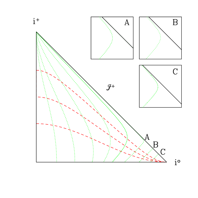
It is now instructive to consider the conformal structure of the MIB hypersurfaces. This is done by applying equations (8) to the standard conformal compactification on Minkowski space, $\tilde{t}\pm\tilde{r}=\tan\left(\left(T\pm R\right)/2\right)$ (where $T$ and $R$ are the axes in the conformal diagram, see Hawking_Ellis or Wald_txt ), and then plotting curves of constant $r$ and $t$. The constant-$t$ hypersurfaces are everywhere spacelike and all reach spatial infinity, ${\rm i^{o}}$. Although constant-$r$ surfaces for $r>r_{\rm c}$ appear at first glance to be null, a closer look (see insets of Fig. 1) reveals that they are indeed everywhere timelike and do not ever reach future null infinity, ${\mathcal{J}^{+}}$.

The equation of motion for the scalar field which results from the action (2) is

$$\frac{1}{\sqrt{|g|}}\partial_{\mu}\left(\sqrt{|g|}g^{\mu\nu}\partial_{\nu}\phi\right)=\phi\left(\phi^{2}-1\right)$$ (13)

which with (9), (10), $\Pi\equiv a\left(\partial_{t}{\phi}-\beta\partial_{r}\phi\right)/\alpha$, and $\Phi\equiv\partial_{r}\phi$ give

$$\dot{\Pi} = \frac{1}{r^{2}b^{2}}\left(r^{2}b^{2}\left(\frac{\alpha}{a}\Phi+\beta\Pi\right)\right)^{\prime}-2\frac{\dot{b}}{b}\Pi-\alpha a\phi\left(\phi^{2}-1\right)$$ (14)

$$\dot{\Phi} = \left(\frac{\alpha}{a}\Pi+\beta\Phi\right)^{\prime}$$ (15)

$$\dot{\phi} = \frac{\alpha}{a}\Pi+\beta\Phi$$ (16)

where  $\dot{}\equiv\partial_{t}$ and  ${}^{\prime}\equiv\partial_{r}$. These equations are familiar from the ADM formalism as applied to the spherically symmetric Klein-Gordon field coupled to the general relativistic gravitational field choptuik:1986 . However, in the current case, instead of a dynamically evolving metric functions, the metric components $a$, $b$, $\alpha$, and $\beta$ are a priori fixed functions of $(t,r)$ that resulted from a coordinate transformation of flat spacetime.

Clearly, characteristic speeds for the massless Klein-Gordon field ($V(\phi)=0$) bound the inward or outward speed (group velocities) of any radiation in a self-interacting field ($V(\phi)\neq 0$). Characteristic analysis of the massless Klein-Gordon equation with metric (9) yields local propagation speeds

$$\lambda_{\pm}=-\beta\pm\frac{\alpha}{a},$$ (17)

where $\lambda_{+}$ and $\lambda_{-}$ are the outgoing and ingoing characteristic speeds, respectively choptuik:1986 ; courant:1962 . For $r\ll r_{\rm c}$, the propagation of scalar radiation in $(t,r)$ or $(\tilde{t},\tilde{r})$ coordinates is essentially identical. However, as illustrated in Fig. 3, and as can be deduced from equations (17) and (10), for $r\approx r_{\rm c}$ both the ingoing and the outgoing characteristic velocities go to zero as $t\rightarrow\infty$ (as the inverse power of $t$). Thus, any radiation incident on this region will effectively be trapped, or “frozen in”. It is this property of the MIB system which enables the effective implementation of non-reflecting boundary conditions. As discussed further in Appendix A, an additional key ingredient is the application of Kreiss-Oliger-style dissipation ko to the difference equations. This dissipation efficiently quenches the trapped outgoing radiation, which as mentioned above tends to be blue-shifted to the lattice scale on a dynamical time-scale.

Finally, we note that, as is evident from Fig. 3, the “absorbing layer” in the MIB system (i.e. the region in which the characteristic speeds are $\approx 0$), expands both outward and inward as $t$ increases. This means that for fixed $r_{c}$, the absorbing layer will eventually encroach on the interior region $r\ll r_{c}$ and ruin the calculation. However, the rate at which the layer expands is roughly logarithmic in $t$, so, in practice, this fact should not significantly impact the viability of the method. For arbitrarily large final integration times, $T$, computational cost will scale as $T\ln T$. However, the calculations described here all used the same values of $r_{c}$ and $r_{\rm max}$, so that for all practical purposes, the computational cost is linear in the integration time.

III The Resonant Structure of Oscillons

Copeland, et al, showed quite clearly that oscillons formed for a wide range of initial bubble radii, $r_{0}$. They even caught a glimpse of the fine structure in the model—which in large part motivated this study—but they did not explore this fine structure of the parameter space in detail. With the efficiency of our new code, we have been able to explore parameter space much more thoroughly, which in turn has yielded additional insights into the dynamical nature of oscillons.

Following gleiser0 we use a gaussian profile for initial data where the field at the core and outer boundary values are set to the vacuum values, $\phi(t,0)\equiv\phi_{c}=1$ and $\phi(t,\infty)\equiv\phi_{o}=-1$ respectively, and the field interpolates between them at a characteristic radius, $r_{0}$:

$$\phi(0,r)=\phi_{o}+\left(\phi_{c}-\phi_{o}\right)\exp\left(-r^{2}/r_{0}^{2}\right).$$ (18)

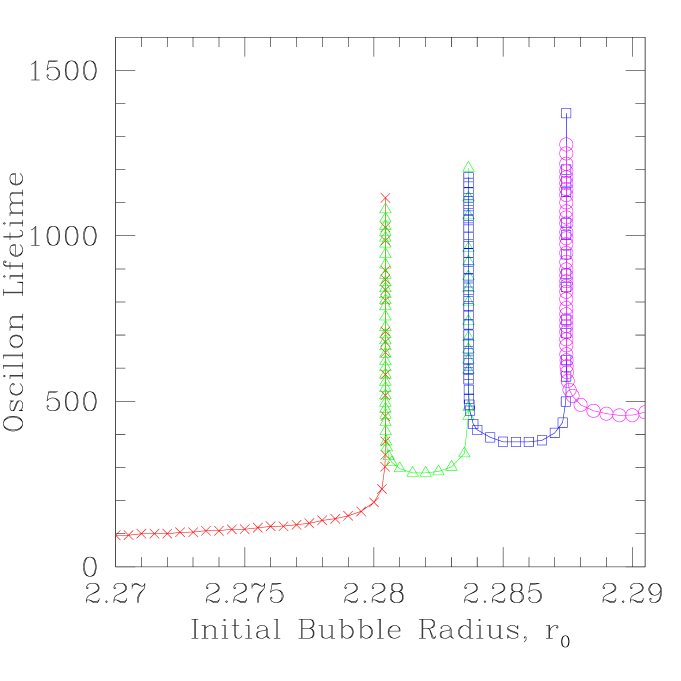
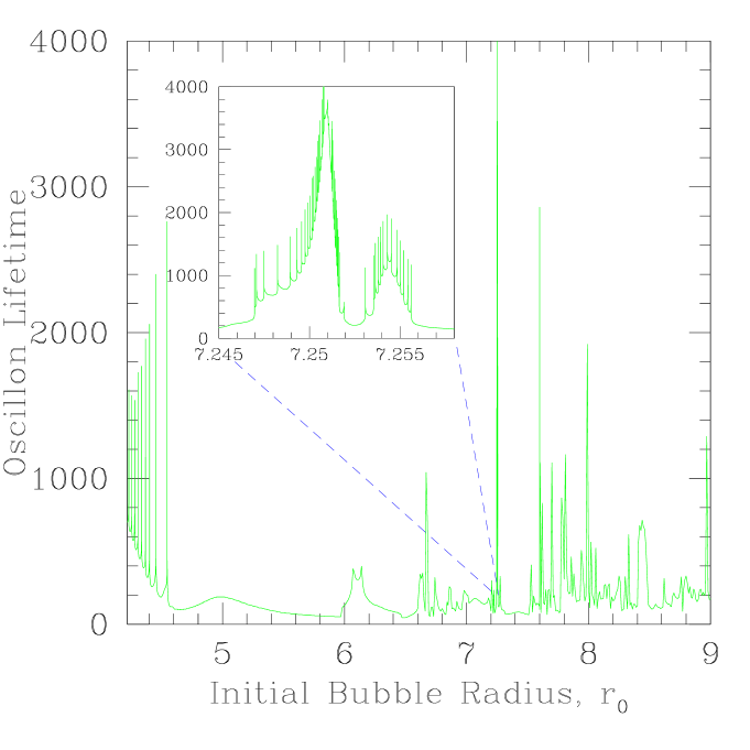
Keeping $\phi_{c}$ and $\phi_{o}$ constant, but varying $r_{0}$, we have a one parameter family of solutions to explore. Figure 4 shows the behavior of oscillon lifetime as a function of $r_{0}$ in the range $2.0\leq r_{0}\leq 5.0$. We discuss three main findings that are distinct from previous work: the existence of resonances and their time scaling properties, the mode structure of the resonant solutions, and the existence of oscillons outside the parameter-space region $2\leq r_{0}\leq 5$.

III.1 Resonances & Time Scaling

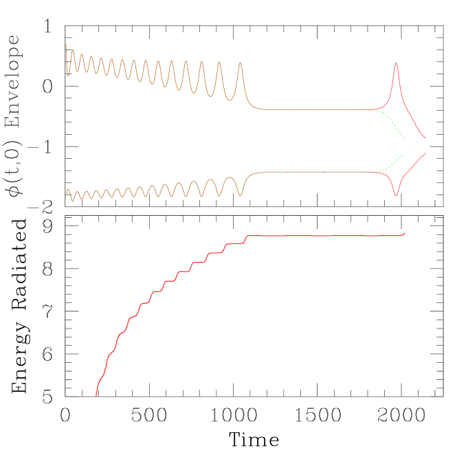
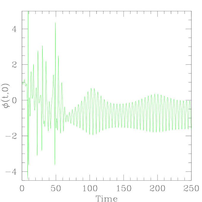
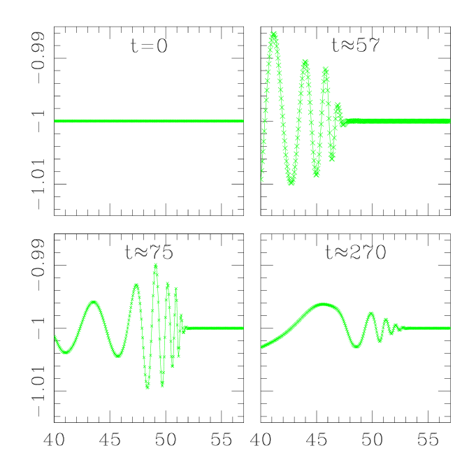
In contrast to Fig. 7 of Copeland et al gleiser1 , the most obvious new feature seen in Fig. 4 is the appearance of the 125 resonances which rise above the overall lifetime profile. These resonances (also seen in Fig. 5) become visible only after carefully resolving the parameter space. Upon fine-tuning $r_{0}$ to about 1 part in $\sim 10^{14}$ we noticed interesting bifurcate behavior about the resonances (Figure 6, top). The field oscillates with a period $T\approx 4.6$ (for all oscillons) so the individual oscillations cannot be seen in the plot, but it is the lower-frequency modulation that is of interest here. The top figure shows the envelope of $\phi(t,0)$ on both sides of a resonance (dotted and solid curves). We see that the large period modulation that exists for all typical oscillons disappears late in the lifetime of the oscillon as $r_{0}$ is brought closer to a resonant value, $r^{\star}_{0}$. On one side of $r^{\star}_{0}$ the modulation returns before the oscillon disperses (refered to as supercritical and shown with the solid curve), while on the other side of $r^{\star}_{0}$ the modulation does not return and the the oscillon simply disperses (refered to as subcritical and shown with the dotted curve). For resonances where $r^{\star}_{0}\lesssim 2.84$, the subcritcal solutions appear on the $r_{0}<r^{\star}_{0}$ side of the resonance and the supercritical solutions appear on the $r_{0}>r^{\star}_{0}$ side of the resonance. The opposite is true for resonances where $r^{\star}_{0}\gtrsim 2.84$, ie. the subcritcal solutions appear on the $r_{0}>r^{\star}_{0}$ side of the resonance and the supercritical solutions appear on the $r_{0}<r^{\star}_{0}$ side of the resonance. This bifurcate behavior does not manifest itself until $r_{0}$ is quite close to $r^{\star}_{0}$. In practice then, to locate a resonant value, $r^{\star}_{0}$, we first maximize the oscillon lifetime using a three point extremization routine (golden section search with bracketing interval of $\sim\!0.62$, NumericalRecipes ) until we have computed an interval whose end-points exhibit the two distinct behaviours just described. Once a resonance has been thus bracketed, we switch to a standard bisection search, and subsequently locate the resonance to close to machine precision. Although we can see from Fig. 6 that the modulation is directly linked to the resonant solution, it is not obvious why this is so. However, if we look at the relationship between the modulation in the field (top) to the power radiated by the oscillon (bottom), we see that they are clearly synchronized.

The behaviour of these resonant solutions may not be surprising to those familiar with the 1+1 $K{\bar{K}}$ scattering studied using the same model 1dkak_campbell . Campbell et al showed that after the “prompt radiation” phase—the initial release of radiation upon collision of a kink and anti-kink—the remaining radiation was emitted from the decay of what they referred to as “shape” oscillations. The “shape modes” were driven by the contribution to the field “on top” of the $K$ and $K^{{}^{{}^{{}_{\!\!\!\!\!\!\rule{6.82864pt}{0.7113pt}}}}}$ soliton solutions. Since the exact closed-form solution for the ideal non-radiative $K{\bar{K}}$ interaction is not known, initial data aimed at generating such an interactionm is generally only approximate, and the “surplus” (or deficit) field is responsible for exciting the shape modes. The energy stored in the shape modes slowly decays away as the kink and antikink interact and eventually the solution disperses.

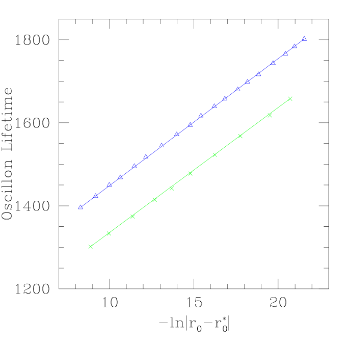
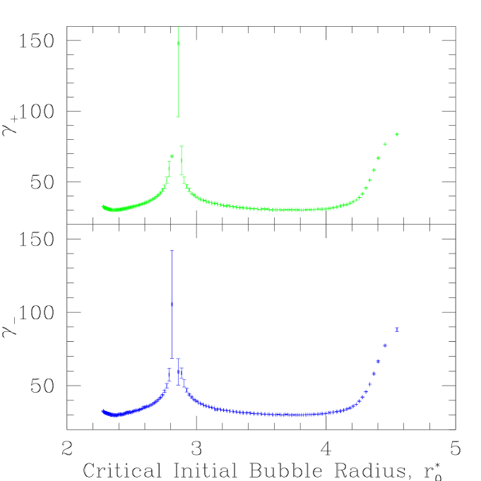
In our case, we believe the large period modulation represents the excitation of a similar “shape mode” superimposed on a periodic, non-radiative, localized oscillating solution. On either side of a resonance in the $r_{0}$ parameter space, the solution is on the threshold of having one more shape mode oscillation. If this is the case, then, as we tune $r_{0}\to r_{0}^{\star}$, we are, in effect, tuning away the single unstable shape mode, and thus should expect that the oscillon lifetime obey a scaling law such as that seen in Type I solutions in critical gravitational collapse TypeI . Figure 7 shows a plot of oscillon lifetime versus $\ln|r_{0}-r_{0}^{\star}|$ (for the $r_{0}=2.335\cdots$ resonance), and we can see quite clearly that there is a scaling law, $T\sim\gamma\ln|r_{0}-r_{0}^{\star}|$, for the lifetime of the solution as measured on either side of the resonance. We denote $\gamma_{+}$ for the scaling exponent on the $r_{0}>r_{0}^{\star}$ side, and $\gamma_{-}$ for the scaling exponent on the $r_{0}<r_{0}^{\star}$ side. Although we observe lifetime scaling for each resonance, the scaling exponent per se varies from resonance to resonance; a plot of the scaling exponents, $\gamma_{+}$ and $\gamma_{-}$, versus the critical initial bubble radius can be seen in Fig. 8. For all resonances we find $\gamma_{+}\approx\gamma_{-}$.

Finally we note that, by analogy with the case of Type I critical gravitational collapse, we expect that the scaling exponents, $\gamma$, are simply the reciprocal Lyapounov exponents associated with each resonance’s single unstable mode. In addition we note that, for any resonance, if we were able to infinitely fine-tune $r_{0}$ to $r_{0}^{\star}$, we would expect the oscillon lifetime to go to infinity.

III.2 Mode Structure

Assuming that periodic, non-radiative solutions to equation (13) exist, we should be able to construct them by inserting an ansatz of the form

$$\phi(t,r)=\phi_{0}(r)+\sum_{n=1}^{\infty}\phi_{n}(r)\cos\left(n\omega t\right)$$ (19)

in the equations of motion and solving the resulting system of ordinary differential equations obtained from matching $\cos\left(n\omega t\right)$ terms:

$$\begin{array}[]{rcl}\left(r^{2}\phi_{0}^{\prime}\right)^{\prime}/r^{2}&=&\phi_{0}\left(\phi_{0}-1\right)\left(\phi_{0}-2\right)\\ &&+\frac{3}{2}\left(\phi_{0}-1\right)\sum\limits_{m}\left(\phi_{m}\right)^{2}\\ &&+\frac{1}{4}\sum\limits_{m,p,q}\phi_{n}\phi_{p}\phi_{q}\left(\delta_{m,\pm p\pm q}\right),\end{array}$$ (20)

$$\begin{array}[]{rcl}\left(r^{2}\phi_{n}^{\prime}\right)^{\prime}/r^{2}&=&\left(3\left(\phi_{0}-1\right)^{2}-\left(n^{2}\omega^{2}+1\right)\right)\phi_{n}\\ &&+\frac{3}{2}\left(\phi_{0}-1\right)\sum\limits_{p,q}\phi_{p}\phi_{q}\left(\delta_{n,\pm p\pm q}\right)\\ &&+\frac{1}{4}\sum\limits_{m,p,q}\phi_{m}\phi_{n}\phi_{q}\left(\delta_{n,\pm m\pm p\pm q}\right).\end{array}$$ (21)

Equations (20) and (21) can also be obtained by inserting ansatz (19) into the action and varying with respect to the $\phi_{n}$ morrisonchat . This set of ODEs can be solved by “shooting”, where the quantities $\phi_{n}(0)$ are the shooting parameters. Unfortunately, we were unable to construct a method that self-consistently computed $\omega$; the best we could achieve was to solve equations (20) and (21) for a given $\omega$ which we measured from the PDE solution.

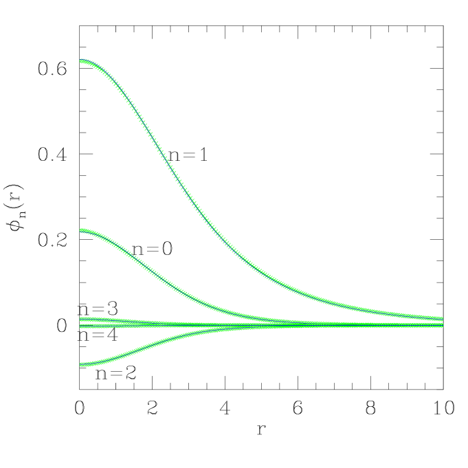
For ease of comparison of the results obtained from the periodic ansatz with those generated via solution of the PDEs, we Fourier decomposed the PDE results. This was done by taking the solution during the interval of time when the large period modulation disappears ($1200<t<1800$ for the oscillon in Fig. 6, for example) and constructing FFTs of $\phi$ at each gridpoint, $r_{i}$. Specifically, at each $r_{i}$, the amplitude of each Fourier mode was obtained from a FFT which used a time series, $\phi(t^{n},r_{i})$, $n=1,2,\,\cdots\,4096$ with $t^{n+1}-t^{n}\equiv\Delta t={\rm constant}$. Keeping only the first five modes in the expansion (19), we compare the Fourier decomposed PDE data with the shooting solution (see Fig. 9). It should be noted that although the value for $\omega$ was determined from the PDE solution, the shooting algorithm still involved a five-dimensional search for the the shooting parameters, $\phi_{n}(0)$, $n=0,\cdots,4$. The close correspondence of the curves shown in Fig 9 strongly suggests that the resonant solutions (ie. in the limit as $r_{0}\rightarrow r_{0}^{\star}$) observed in the PDE calculations are indeed consistent with the periodic, non-radiative oscillon ansatz (19).

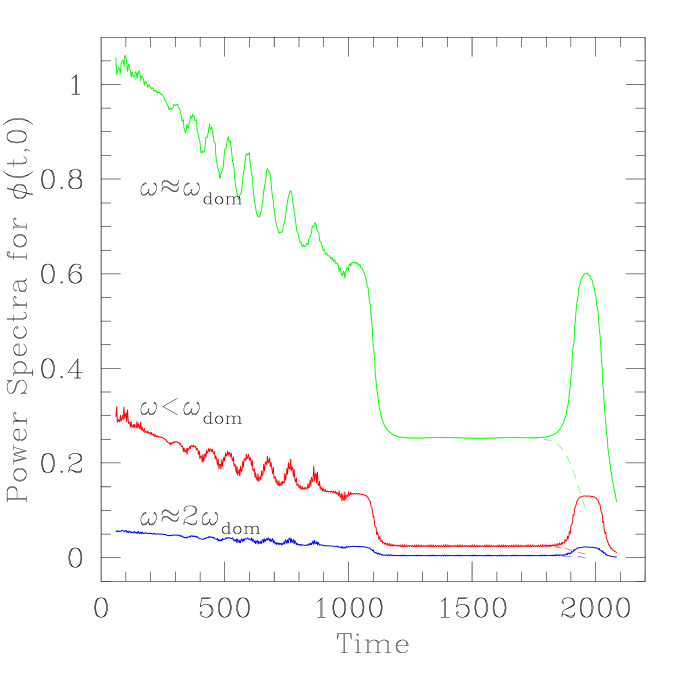
By examining the three most dominant components of the power spectrum of $\phi(t,0)$, Fig. 10, we can see that during the “no-modulation” epoch, the amplitude of each Fourier mode becomes constant. Although the specific plot is for the core amplitude, $r=0$, we note that this behavior holds for all $r$. Again, this is consistent with the view that as we tune $r_{0}$ to $r_{0}^{\star}$, the oscillon phase of the evolution is better and better described by a one-mode unstable, “intermediate attractor”. As discussed previously, this is precisely reminiscent of the Type I critical phenomena studied in critical gravitational collapse, particularly the collapse of a real, massive scalar field as studied by Brady et al TypeI , where the intermediate attractors are unstable, periodic, “oscillon stars” discovered earlier by Seidel and Suen SeidelSuen .

III.3 (Bounce) Windows to more Oscillons

Lastly, we consider the existence of oscillons generated by gaussian initial data with $r_{0}\gtrsim 5$. The oscillons explored by Copeland et al, were restricted to the parameter-space region, $2\lesssim r_{0}\lesssim 5$, and in fact it was concluded that there was an upper bound, $r_{0}\sim 4.2$, beyond which evolution of gaussian data would not result in an oscillon phase newgleiser . However, we have found that oscillons can form for $r_{0}\gtrsim 5$, and that they do so by a rather interesting mechanism.

Again, from the 1+1 dimensional $K{\bar{K}}$ scattering studies of Campbell et al, it is well known that a kink and antikink in interaction often “bounce” many times before either dispersing or falling into an (unstable) bound state. Here, a bounce occurs when the kink and antikink reflect off one another, stop after propagating a short distance, then recollapse.

We find that such behaviour occurs in the (3+1) dimensional case as well, but now the unstable bound state is an oscillon. For larger $r_{0}$, instead of remaining within $r\lesssim 2.5$ after reflection through $r=0$ (as occurs for $2\lesssim r_{0}\lesssim 5$), the bubble wall travels out to larger $r$ (typically $3\lesssim r\lesssim 6$), stops, then recollapses, shedding away large amounts of energy in the process (see Fig. 11). Thus in this system, as with the 1+1 $K{\bar{K}}$ model, there are regions of parameter space which constitute “bounce windows”. Within such regions, the bounces allow the bubble to radiate away large amounts of energy. The bubble then recollapses, effectively producing a new initial configuration (albeit with a different shape) with a smaller effective $r_{0}$. Within these “windows” both oscillons and resonances (similar to those observed for $2\lesssim r_{0}\lesssim 4.6$) can be observed (inset of Fig. 12).

IV Conclusions

Using a new technique for implementing non-reflecting boundary conditions for finite-differenced evolutions of non-linear wave equations, we have conducted an extensive parameter space survey of bubble dynamics described by a spherically-symmetric Klein-Gordon field with a symmetric double-well potential. We have found that the parameter space of the model exhibits resonances, wherein the lifetimes of the intermediate-phase “oscillons” diverge as one approaches a resonance. We have conjectured that these resonances are single-mode unstable solutions, analogous to Type I solutions in critical gravitational collapse, and have presented evidence that their lifetimes satisfy the type of scaling law which is to be expected if this is so.

In addition, we have independently computed resonant solutions starting from an ansatz of periodicity, and have demonstrated good agreement between the solutions thereby computed, and those generated via finite-difference solution of the PDEs. Finally, we have showed that oscillons can form from bubbles with energies higher than had previously been assumed, through a mechanism analogous to the bounce windows found in the $1+1$ case of kink-antikink scattering.

We note that the use of MIB or related coordinates, in conjunction with finite-difference dissipation techniques, should result in a generally-applicable strategy for formulating non-reflecting boundary conditions for finite-difference solution of wave equations. The method has already been used in the study of axisymmetric oscillon collisions Thesis , and attempts are underway to use similar techniques in the context of 3-D numerical relativity and 2-D and 3-D ocean acoustics.

V Acknowledgments

We thank Philip J. Morrison for useful discussions on the exact non-radiative oscillon solutions. We also thank Marcelo Gleiser and Andrew Sornborger for useful input on many oscillon issues. This research was supported by NSF grant PHY9722088, a Texas Advanced Research Projects Grant, and by NSERC. The bulk of the computations described here were carried out on the vn.physics.ubc.ca Beowulf cluster, which was funded by the Canadian Foundation for Innovation, with operations support from NSERC, and from the Canadian Institute for Advanced Research. Some computations were also carried out using the Texas Advanced Computing Center’s SGI Cray SV-1 aurora.hpc.utexas.edu and SGI Cray T3E lonestar.hpc.utexas.edu.

Appendix A Finite Difference Equations

Equations (14,15,16) are solved using two-level second order (in both space and time) finite difference approximations on a static uniform spatial mesh:

$$r_{i}=\left(i-1\right)\,\Delta r,\quad i=1,2,\cdots I$$ (22)

where $I$ is the total number of mesh points

$$\Delta r=\frac{r_{\rm max}}{I-1}\,.$$ (23)

The scale of discretization is set by $\Delta r$ and $\Delta t=\lambda\Delta r$, where we fixed the Courant factor, $\lambda$, to $0.5$ as we changed the base discretization.

Using the operators from Table 1, $\partial_{r}\tilde{r}=a$, $\partial_{r}=nr^{n-1}\partial_{r^{n}}$, and $rb=\tilde{r}$, the difference equations applied in the interior of the mesh, $i=2,3,\cdots I-1$, are

$$\begin{array}[]{rcl}\displaystyle{\Delta^{d}_{t}\Pi^{n}_{i}}&=&\displaystyle{3\mu_{t}\left[a\Delta_{\tilde{r}^{3}}\left(\tilde{r}^{2}\left(\frac{\alpha}{a}\Phi+\beta\Pi\right)\right)\right]^{n}_{i}}\\ &&\displaystyle{-2\mu_{t}\left(\frac{\dot{b}}{b}\Pi-\alpha a\phi\left(\phi^{2}-1\right)\right)^{n}_{i}},\end{array}$$ (24)

$$\Delta^{d}_{t}\Phi^{n}_{i}=\mu_{t}\Delta_{r}\left(\frac{\alpha}{a}\Pi+\beta\Phi\right)^{n}_{i},$$ (25)

$$\Delta^{d}_{t}\phi^{n}_{i}=\mu_{t}\left(\frac{\alpha}{a}\Pi+\beta\Phi\right)^{n}_{i}.$$ (26)

These equations are solved using an iterative scheme and explicit dissipation of the type advocated by Kreiss and Oliger ko . The dissipative term, incorporated in the operator $\Delta^{d}_{t}$, is essentially a fourth spatial derivative multiplied by $\left(\Delta r\right)^{3}$ so that the truncation error of the difference scheme remains $O(\Delta r^{2},\Delta t^{2})$. The temporal difference operator, $\Delta^{d}_{t}$, is used as an approximation to $\partial_{t}$ everywhere in the interior of the computational domain, except for next-to-extremal points, where $\Delta_{t}$ is used because the grid values $f^{n}_{i+2}$ or $f^{n}_{i-2}$ are not defined.

At the inner boundary, $r=0$, we use $O(\Delta r^{2})$ forward spatial differences to evolve $\Pi$

$$\mu_{t}\left(\Delta^{f}_{i}\Pi-\displaystyle{\frac{a^{\prime}}{a}\Pi}\right)^{n}_{1}=0.$$ (27)

whereas $\Phi^{n}_{1}$ is fixed by regularity:

$$\Phi^{n}_{1}=0.$$ (28)

To update $\phi$, we use a discrete versions of the equation for ${\dot{\phi}}$ which follows from the definition of $\Pi$:

$$\Delta_{t}\phi=\mu_{t}\left(\frac{\alpha\Pi}{a}+\beta\Phi\right)^{n}_{i}\quad\quad i=1,2,\cdots I$$ (29)

At the outer boundary, $r=r_{\rm max}$, our specific choice of boundary conditions and discretizations thereof have little impact; due to the use of MIB coordinates and Kreiss-Oliger dissipation, almost none of the outgoing scalar field reaches the outer edge of the computational domain. Nevertheless, we imposed discrete versions of the usual Sommerfeld conditions for a massless scalar field on $\Pi$ and $\Phi$:

$$\Delta_{t}\Pi^{n}_{i}+\mu_{t}\left(\Delta^{b}_{r}\Pi+\frac{\Pi}{r}\right)^{n}_{I}=0,$$ (30)

$$\Delta_{t}\Phi^{n}_{i}+\mu_{t}\left(\Delta^{b}_{r}\Phi+\frac{\Phi}{r}\right)^{n}_{I}=0,$$ (31)

Appendix B Testing the MIB Code

One might think that “freezing” outgoing radiation on a static uniform mesh would lead to a “bunching-up” of the wave-train from the oscillating source, which would then result in a loss of resolution, numerical instabilities, and an eventual breakdown of the code. However, this turns out not to be the case; all outgoing radiation is “frozen” around $r\approx r_{\rm c}$, but the steep gradients which subsequently form in this region are efficiently and stably annihilated by the dissipation which is explicitly added to the difference scheme.

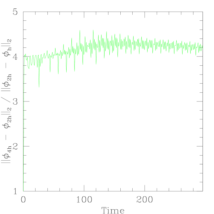
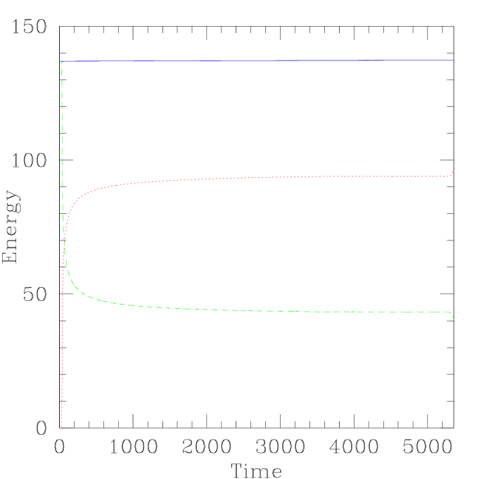
In fact, there is a loss of resolution and second order convergence for $r\sim r_{\rm c}$, but this does not affect the stability or convergence of the solution for $r\ll r_{\rm c}$. Figure (14) shows a convergence test for the field $\phi$ for $r<r_{\rm c}/2$ over roughly six crossing times. Since we are solving equation (13) in flat spacetime, it is very simple to monitor energy conservation. The spacetime admits a timelike Killing vector, $t^{\nu}$, so we have a conserved current, $J_{\mu}\equiv t^{\nu}T_{\mu\nu}$. We monitor the flux of $J_{\mu}$ through a surface constructed from two adjacent spacelike hypersurfaces for $r\leq r_{\rm c}$ (with normals $n_{\mu}=(\pm 1,0,0,0)$), and an “endcap” at $r=r_{O}$ (with normal $n^{\mu}=(0,a^{-1},0,0))$. To obtain the the conserved energy at a time, $t_{f}$, the energy contained in the bubble,

$$E_{\rm bubble}=4\pi\int\limits_{0}^{\ \ \ r_{O}}r^{2}b^{2}\left(\frac{\Pi^{2}+\Phi^{2}}{2a^{2}}+V(\phi)\right)dr,$$ (32)

(where the integrand is evaluated at time $t_{f}$) is added to the total radiated energy,

$$E_{\rm rad}=4\pi\int\limits_{0}^{\ t_{f}}r^{2}b^{2}\frac{\Pi\Phi}{a^{2}}dt$$ (33)

(where the integrand is evaluated at $r=r_{O}$). The sum, $E_{\rm total}=E_{\rm bubble}+E_{\rm rad}$, remains conserved to within a few tenths of a percent through a quarter million iterations (see Fig. (15)).

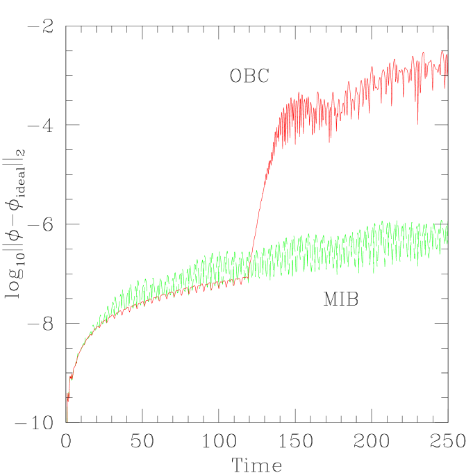
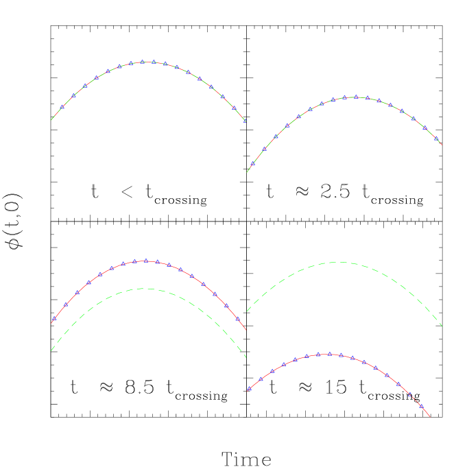
Although monitoring energy conservation is a very important test, it says little about whether there is reflection of the field off of the outer boundary, $r=r_{\rm max}$, or the region $r\approx r_{\rm c}$. To check the efficacy of our technique for implementing non-reflecting boundary conditions, we compare the MIB results to those obtained with two other numerical schemes. The first alternate method involves evolution of equation (13) in ($\tilde{t}$,$\tilde{r}$) coordinates on a grid with $r_{\rm max}$ sufficiently large that radiation never reaches the outer boundary (large-grid solutions). For a given discretization scale, results from this approach serve as near-ideal reference solutions, since the solution is guaranteed to be free of contamination from reflection off the outer boundary. The second method involves evolution on a grid with the same $r_{\rm max}$ adopted in the MIB calculation, but with discrete versions of massless Sommerfeld (outgoing radiation) conditions applied at $r=r_{\rm max}$. We refer to the results thus generated as OBC solutions, and since we know that these solutions do have error resulting from reflections from $r=r_{\rm max}$, they demonstrate what can go wrong when a solution is contaminated by reflected radiation. Treating the large-grid solution as ideal, Fig. (16) compares typical $\log_{10}||\phi-\phi_{\rm ideal}||_{2}$ for the MIB and OBC solutions. There is a steep increase in the OBC solution error (three orders of magnitude) around $t=125$, which is at roughly two crossing times. This implies that some radiation emitted from the initial collapse reached the outer boundary and reflected back into the region $r<r_{O}$. There is no such behavior found in any MIB solutions. Lastly, for a more direct look at the field itself, we can see $\phi(t,0)$ for large-grid (triangles), MIB (solid curves), and OBC (dashed curves) solutions in Fig. (17). Initially, both the MIB and OBC solutions agree with the large-grid solution extremely well. However, after two crossing times the OBC solution starts to substantially diverge from the ideal solution, while the MIB results remain in very good agreement with the ideal calculations.

In summary, the MIB solution conserves energy, converges quadratically in the mesh spacing (as expected), and produces results which are equivalent—at the level of truncation error—to large-grid reference solutions. At the same time, the MIB approach is considerably more computationally efficient than dynamical- or large-grid techniques.

Operator	Definition	Expansion
$\Delta^{f}_{r}f^{n}_{i}$	$\left(-3f^{n}_{i}+4f^{n}_{i+1}-f^{n}_{i+2}\right)/2\Delta r$	$\partial_{r}f\big{|}^{n}_{i}+O\left(\Delta r^{2}\right)$
$\Delta^{b}_{r}f^{n}_{i}$	$\left(3f^{n}_{i}-4f^{n}_{i-1}+f^{n}_{i-2}\right)/2\Delta r$	$\partial_{r}f\big{|}^{n}_{i}+O\left(\Delta r^{2}\right)$
$\Delta_{r}f^{n}_{i}$	$\left(f^{n}_{i+1}-f^{n}_{i-1}\right)/2\Delta r$	$\partial_{r}f\big{|}^{n}_{i}+O\left(\Delta r^{2}\right)$
$\Delta_{t}f^{n}_{i}$	$\left(f^{n+1}_{i}-f^{n}_{i}\right)/\Delta t$	$\partial_{t}f\big{|}^{n+\frac{1}{2}}_{i}+O\left(\Delta t^{2}\right)$
$\Delta^{d}_{t}f^{n}_{i}$	$\left(f^{n+1}_{i}-f^{n}_{i}\right)/\Delta t+$	$\partial_{t}f\big{|}^{n+\frac{1}{2}}_{i}+O\left(\Delta t^{2}\right)$
	$\epsilon_{dis}[6f^{n}_{i}+f^{n}_{i-2}+f^{n}_{i+2}-$
	$4\left(f^{n}_{i-1}+f^{n}_{i+1}\right)]/16\Delta t$
$\mu_{t}f^{n}_{i}$	$\left(f^{n+1}_{i}+f^{n}_{i}\right)/2$	$f\big{|}^{n+\frac{1}{2}}_{i}+O\left(\Delta t^{2}\right)$

Table 1: Two-Level Finite Difference Operators. Here we have adopted a standard finite-difference notation: $f^{n}_{i}\equiv f((n-1)\Delta t,(i-1)\Delta r)$

Figure 1: Conformal diagram showing surfaces of constant $r$ (dotted lines) and lines of constant $t$ (dashed lines). Lines of constant $t$ look exactly like the constant-$t$ hypersurfaces of Minkowski space, whereas the lines of constant $r$ behave much differently. For $r>r_{c}$, it appears as if the constant-$r$ surfaces are null. However, as insets A, B, and C show, the constant-$r$ lines do not become null (do not intersect future null infinity), but rather are everywhere timelike.

Figure 2: Plot of the characteristic velocities as a function of the MIB coordinates, $r^{\prime}$ and $t^{\prime}$ in units where $r_{c}$ is set to unity. $\lambda_{+}$ and $\lambda_{-}$ are the outgoing and ingoing characteristic speeds respectively. $\delta$ is taken to be $\delta\rightarrow\delta/r_{c}\approx 0.0893$ (corresponding to the system used in this article). Characteristic velocities are plotted for times $t^{\prime}=0$, $1$, $10$, and $100$ ($t^{\prime}=100$ is larger than the lifetime of the longest lived solution studied in this work). As $r\to 1$, we have $\lambda_{\pm}(t^{\prime},r^{\prime})=O(1/t^{\prime})$.

Figure 3: Plot of characteristic speeds, $\lambda_{\pm}(r^{\prime},100)$, where $r^{\prime}$ and $t^{\prime}$ are radial MIB coordinates in units where $r_{c}$ is set to unity.

Figure 4: Plot of oscillon lifetime versus initial bubble radius for $2.0\leq r_{0}\leq 5.0$. Each of the 125 resonances is resolved to one part in $10^{14}$.

Figure 5: Plot of oscillon lifetime versus initial bubble radius for $2.27\leq r_{\rm initial}\leq 2.29$. The three resonances shown occur at $r^{*}_{0}\approx 2.2805$, $r^{*}_{1}\approx 2.2838$, and $r^{*}_{2}\approx 2.2876$. Each resonance separates the parameter space into regions with $n$ and $n+1$ modulations; the x’s correspond to oscillons with no modulations, the triangles to oscillons with one modulation, the squares to two modulations, and the circles to three modulations.

Figure 6: Top plot shows the envelope of $\phi(t,0)$ for $r^{\star}_{0}\!\pm\!\Delta r_{0}$ displaying bifurcate behavior around the $r^{\star}_{0}\approx 2.335$ resonance ($\Delta r_{0}\sim 10^{-14}$); the solid curve is the envelope barely above resonance (15 modulations) while the dotted line is the envelope barely below resonance (14 modulations). Bottom plot shows the energy radiated as a function of time through the surface containing the oscillon as defined in Appendix B. The increases in the energy radiated are synchronized with the modulation in the field.

Figure 7: Plot of time scaling, $T$ versus $\ln|r_{0}-r_{0}^{\star}|$ for the $r_{0}\approx 2.335$ resonance. The top line (triangles) displays the scaling behavior for supercritical evolutions, $r_{0}>r_{0}^{\star}$, while the bottom line (x’s) shows the scaling for subcritical calculations, $r_{0}<r_{0}^{\star}$. The exponents (measured by the slopes of the lines) are both approximately equal to $\gamma=30$. The offset in the two curves represents the time spent by supercritical oscillons in executing the final modulation shown in Fig. 6.

Figure 8: Plot of critical exponents for each resonance. There are two values of $\gamma$ for each resonance. The top plot displays the $\gamma_{+}$ vs. $r_{0}^{\star}$ while the lower plot displays $\gamma_{-}$ vs. $r_{0}^{\star}$. The uncertainties are estimated from running the entire parameter space surveys at two resolutions, $N\equiv N_{r}=1449$ and $N^{\prime}\equiv N_{r}^{\prime}=1025$ and estimating the error, $\Delta\gamma=|\gamma_{N}-\gamma_{N^{\prime}}|$.

Figure 9: Critical solution $\phi_{n}(r)$ (for $n=0,1,2,3,4$) obtained from the Fourier-decomposed PDE data (x’s) overlayed with $\phi_{n}(r)$ obtained by shooting equations 20 and 21 (solid curves). The Fourier-decomposed PDE data overlays the shooting solution everywhere.

Figure 10: Power spectra of the core amplitude, $\phi(t,0)$, for the oscillons barely above and below the $r_{0}\approx 2.335$ resonance. The power measured in each frequency regime slowly diminishes as the oscillon radiates away much of its energy until approximately $t=1100$ where the oscillon enters a non-radiative state and all the components of the power spectrum become constant.

Figure 11: Plot of $\phi(t,0)$ for $r_{0}=7.25$ displaying extremely nonlinear and unpredictable behavior during the “bouncing” phase (for $t<60$), after which the field settles into a typical oscillon evolution. Once in the oscillon regime, the period is approximately $T\approx 4.6$, and the first two modulations of the field can be seen (envelope maxima at $t\approx 105$ and $t\approx 200$).

Figure 12: Plot of oscillon lifetime versus initial radius of bubble for $4.22\leq r_{0}\leq 9$. Although there seem to be no oscillons in the range $4.6\lesssim r_{0}\lesssim 6$, it is clear that oscillons and resonances do exist for higher initial bubble radii, $r_{0}\gtrsim 6.5$.

Figure 13: Fundamental field $\phi(r)$ in the freeze-out region at $t=0,\ 57,\ 75,\ {\rm and}\ 270$. The characteristic speeds of the radiation $\to 0$ as $r\to r_{c}$ (here, $r_{c}=56$) and the wavelength of the radiation is blue-shifted to the lattice Nyquist limit, $2\Delta r$. The Kreiss-Oliger dissipation explicitly added to the finite difference equations subsequently “quenches” the field.

Figure 14: Convergence factor, $C_{f}=||\phi_{4h}-\phi_{2h}||_{2}/||\phi_{2h}-\phi_{h}||_{2}$, for the field $\phi$ composed from the solution at three different discretizations (value of 4 indicates 2nd order convergence). The $\ell_{2}$ norm $||\cdots||_{2}$ is defined by $||v||_{2}=\left(N^{-1}\sum_{i=1}^{N}v_{i}\right)^{1/2}$

Figure 15: Plot of energy contained in oscillon (dashed line), energy radiated (dotted line), and total energy (solid line). The total energy of the system is a constant of motion and is numerically conserved to within a few tenths of a percent. The energy contained within the bubble drops rapidly during the initial radiative phase and plateaus around $E\approx 43m/\lambda$ during the quasi-stable “oscillon” phase.

Figure 16: Plot comparing the OBC (solid line) and MIB (dashed line) solutions to an “ideal” solution. The OBC solution is obtained using a massless outgoing boundary condition, the MIB solution is obtained by solving the system in spherical MIB coordinates, and the ideal solution is obtained by evolving the solution in standard ($r$,$t$) coordinates on a grid large enough to ensure no reflection off the outer boundary. The error estimates are obtained from the $\ell_{2}$-norm of the difference between the trial solutions (OBC or MIB) and the ideal solution, $||\phi-\phi_{\rm ideal}||_{2}$. Contamination of the OBC solution is observed at two crossing times, $t\approx 120$, where the error estimate increases by over three orders of magnitude. The MIB solution error grows slowly and steadily as expected when solving a continuum equation with two different finite difference techniques.

Figure 17: $\phi(t,0)$ versus time for the large-grid solution (triangles), MIB solution (solid curves), and OBC solution (dashed curves). The solutions all agree before $2t_{\rm crossing}$, but the OBC solution begins to drift away from the ideal solution after $2t_{\rm crossing}$. The error in the OBC solution is due to radiation that is reflected off of the outer boundary (hence needing two crossing times to return to $r=0$ to contaminate the oscillon). All pictures span the same area, $\Delta\phi=0.075$ by $\Delta t=0.5$.

References

- (1)
- (2) J.S. Russell, Report of the fourteenth meeting of the British Association for the Advancement of Science, London, 1845.
- (3) A. Vilenkin, Phys. Rep. 121 263-315 (1985).
- (4) R. Friedberg, T.D. Lee, and A. Sirlin, Phys. Rev. D 13 2739-2761 (1976).
- (5) S. Coleman, Nucl. Phys. B 262, 263-283 (1985).
- (6) I.L. Bogolyugskii, and V.G. Makhan’kov, JETP Letters 24, 12 (1976).
- (7) I.L. Bogolyugskii, and V.G. Makhan’kov, JETP Letters 25, 107 (1977).
- (8) M. Gleiser, Phys. Rev. D49, 2978-2981 (1994).
- (9) E.J. Copeland, M. Gleiser, and H.R. Müller, Phys. Rev. D52, 1920-1932 (1995). Also available as hep-ph/9503217.
- (10) D.K. Campbell, J.F. Schonfeld, and C. A. Wingate, Physica 9D, 1-32 (1983).
- (11) M. Gleiser and A. Sornborger, Phys. Rev. E62, 1368-1374 (2000). Also available as patt-sol/9909002.
- (12) H.-O. Kreiss and J. Oliger, Methods for the Approximate Solution of Time Dependent Problems, Global Atmospheric Research Program Publication No. 10, World Meteorological Organization, Case Postale No. 1, CH-1211 Geneva 20, Switzerland (1973).
- (13) M.W. Choptuik, T. Chmaj and P. Bizoń, Phys. Rev. Lett., 77, 424-427 (1996); C.M. Chambers, P.R. Brady, and S.M.C.V. Goncalves, Phys. Rev. D56 , 6057 (1997); S.H. Hawley and M.W. Choptuik, Phys. Rev. D62:104024 (2000).
- (14) R. Arnowitt, S. Deser and C.W. Misner, in Gravitation: An Introduction to Current Research, L. Witten ed., Wiley, New York (1962); C.W. Misner, K.S. Thorne and J.A. Wheeler, Gravitation, W.H. Freeman, San Francisco (1973).
- (15) S.W. Hawking and G. Ellis, The Large Scale Structure of Space-Time, Cambridge University Press, Cambridge, 1973.
- (16) R. Wald, General Relativity, The University of Chicago Press, Chicago, 1984.
- (17) M.W. Choptuik, Ph.D. Dissertation, The University of British Columbia, 1986.
- (18) R. Courant and D. Hilbert, Methods of Mathematical Physics Volume II (Wiley and Sons, New York, 1962).
- (19) W.H. Press, S.A. Teukolsky, W.T. Vetterling, and B.P. Flannery, Numerical Recipes in C, 2nd Edition, Cambridge University Press, Cambridge, 1994.
- (20) P.J. Morrison, Personal communications (1999-2000).
- (21) E. Seidel and W.-M. Suen, Phys. Rev. Lett. 66, 1659-1662 (1991)
- (22) E.P. Honda, PhD Dissertation, The University of Texas at Austin, (2000) (unpublished)