QCD thermodynamics at finite density

Abstract

Recent progress in extending finite temperature lattice QCD simulations from the $T$ axis into the finite density plane is reviewed. The covered topics are a calculation of the transition line by multidimensional reweighting, screening mass calculations in dimensionally reduced QCD and simulations at imaginary $\mu$.

1 Introduction

QCD at finite baryon density plays a role in nature in two rather different regimes: It occurs in heavy ion collisions whose initial state has non-zero baryon number, and whose subsequent plasma state is of high temperature and low density. It is also believed to constitute the core of neutron stars, consisting of cold and very dense matter. These two situations correspond to the regions close to the axes in the tentative QCD phase diagram Fig. 1.

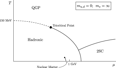
Figure 1: Qualitative phase diagram for QCD with two massless flavours. On the $T$ axis and along the dashed line there is a crossover, solid lines mark first order transitions. The tricritical point is expected to move closer to the $T$ axis for finite $m_{s}$. From [1].

Here the interest is in the former regime, whose understanding is particularly pressing in view of experiments at SPS, LHC (CERN) and RHIC (BNL).

In order to come to first principles predictions, non-perturbative methods are required. Unfortunately, lattice QCD has so far failed to be a viable tool for the analysis because of the so-called “sign-problem”. The QCD partition function is given by

$$Z=\int DU\,\det M(\mu){\rm e}^{-S_{YM}[U]},$$ (1)

where $S_{YM}$ is the pure gauge action and $\det M(\mu)$ denotes the fermion determinant. For the gauge group SU(3) and $\mu\neq 0$, $\det M$ is complex and prohibits standard Monte Carlo importance sampling, for which a manifestly positive measure in the functional integral is required. While still no ab initio solution of the sign problem is available, recent results suggest that at finite temperatures around the deconfinement transition and for low densities the sign problem is milder and simulations are possible. This contribution reviews some recent progress obtained by reweighting methods and simulations of dimensionally reduced QCD. It also discusses what we can learn from QCD with imaginary chemical potential where the integration measure is real and no reweighting is necessary. For a more complete coverage and references to other approaches see e.g. [2].

2 Reweighting methods

The Glasgow method [3] evaluates the partition function by absorbing the complex determinant into the observable, and doing the importance sampling with the positive part of the measure,

$$Z=\left\langle\frac{\det M(\mu)}{\det M(\mu=0)}\right\rangle_{\mu=0}\;.$$ (2)

However, numerical results give for the onset of baryon density on the $\mu$ axis the unphysical value $\mu_{0}=m_{\pi}/2$ instead of the expected $\mu_{0}=m_{B}/3$, which is also the pathological behaviour of the quenched theory [4]. The reason for this failure is the poor overlap between the Monte Carlo ensemble of configurations at $\mu=0$ used to compute averages by reweighting, and the full ensemble at $\mu\neq 0$.

This situation can be improved by splitting the determinant in modulus and phase, $\det M=|\det M|\exp({\rm i}\phi)$, and incorporating the modulus into the measure, while only the phase is used for reweighting [5],

$$Z=\left\langle{\rm e}^{{\rm i}\phi}\right\rangle_{|\det M|}\;.$$ (3)

The expectation value of the phase factor can be viewed as a ratio of two partition functions, one of the full theory and one with only the positive modulus of the determinant in its measure. It thus behaves as $\exp(-\Delta F)$, where the exponent is the free energy difference and an extensive quantity. Consequently, $\langle\exp({\rm i}\phi)\rangle\sim\exp(-V)$, whose measurement requires exponentially large statistics for realistic volumes.

Recently considerable progress has been reported by means of a two-dimensional reweighting method [6], which in addition to $\mu$ also reweights in the lattice gauge coupling $\beta$, rewriting the partition function as

$$Z=\left\langle\frac{{\rm e}^{-S_{YM}(\beta)}\det(M(\mu))}{{\rm e}^{-S_{YM}(\beta_{0})}\det(M(\mu=0))}\right\rangle_{\mu=0,\beta_{0}}.$$ (4)

The simulation performed in [6] for 2+1 flavours of staggered quarks is concerned with the critical line and the endpoint of the deconfinement phase transition. The simulation parameters are tuned such as to stay on the (pseudo-)critical line defined by the location of Lee Yang zeros. While reweighting only in $\mu$ would inevitably employ an ensemble away from criticality, the second parameter can be used to keep the Monte Carlo ensemble fluctuating between the phases, as the full ensemble certainly would. This simulation constitutes the first numerical prediction of the $(\mu,T)$ phase diagram and is displayed in Fig. 2.

Figure 2: Phase diagram for 2+1 flavour QCD ($m_{\pi}$ is about four times its physical value, $m_{s}\sim 10m_{u}$). From [6].

However, it still has some caveats, and more work is required to confirm these results. The lattices are still rather coarse ($a\sim 0.3fm)$ and the volumes small. Since the sign problem becomes exponentially stronger with the volume, it remains to be seen whether infinite volume and continuum limits can be taken with this method. More importantly, while the two-dimensional reweighting on the critical line does sample both phases, there is no guarantee that it has a good overlap with the full ensemble, which is still at a different point of parameter space. Hence it seems important to cross check these results by a different method.

3 Imaginary chemical potential

There are a number of suggestions to consider imaginary chemical potential, for which the integration measure is positive and simulations are straightforward. The connection to real chemical potential is provided by the canonical partition function at fixed quark number $Q$, which is related to the grand canonical partition function at fixed imaginary chemical potential by [7, 8]

$$Z(T,Q)=\int_{-\pi T}^{+\pi T}\frac{d\mu_{I}}{2\pi T}\,Z(T,\mu={\rm i}\mu_{I})\,e^{-i\mu_{I}Q/T}.$$ (5)

One proposal is to simulate $Z$ for various values of $\mu_{I}$, and then numerically do the Fourier integration [9]. This becomes more and more difficult, however, for large $Q$, and extrapolation to the thermodynamic limit seems questionable. The method has been tested in the two-dimensional Hubbard model [9] but not for QCD.

Another proposal, to be further pursued in the following, is to use analyticity of the partition function to continue expectation values computed with $Z({\rm i}\mu,T)$. Not too far from the temperature axis (and away from a phase transition), physical quantities are analytic functions of $\mu/T$ having a Taylor series. One can then fit the coefficients of the truncated series to results obtained at imaginary $\mu$ and analytically continue the series to real $\mu$. This has been explored for the chiral condensate in the strong coupling limit [10]. In the following it will be tested non-perturbatively in the deconfined phase in the framework of an effective theory.

4 Dimensionally reduced QCD

For temperatures larger than a few times the deconfinement temperature $T_{c}$, the static (equilibrium) physics of QCD can be accurately described by an effective theory, which indeed permits simulations with non-vanishing real quark chemical potential $\mu/T\mathop{\raise 1.29167pt\hbox{$<$\kern-7.5pt\raise-4.73611pt\hbox{$\sim$}}}4.0$, where the sign problem sets in [11]. It permits to study any number of quarks with small or zero mass. The domain of parameter space where the approach is applicable contains the phenomenologically relevant region in which heavy ion collisions are operating. At and above SPS energies, densities in heavy ion collisions are estimated to be $\mu_{B}/T\mathop{\raise 1.29167pt\hbox{$<$\kern-7.5pt\raise-4.73611pt\hbox{$\sim$}}}4.0$ [12], i.e. a quark chemical potential $\mu/T\mathop{\raise 1.29167pt\hbox{$<$\kern-7.5pt\raise-4.73611pt\hbox{$\sim$}}}1.3$, which is well within the range where simulations are feasible.

Equilibrium physics is described by euclidean time averages of gauge invariant operators, $\bar{A}({\bf x})=T\int_{0}^{1/T}d\tau\,A(\bf{x},-{\rm i}\tau)$. Their spatial correlation functions

$$C(|{\bf x}|)=\langle\bar{A}({\bf x})\bar{A}(0)\rangle_{c}\sim{\rm e}^{-M|{\bf x}|},$$ (6)

decay exponentially with distance. The “screening masses” $M$ correspond to the inverse length scale over which the equilibrated medium is sensitive to the insertion of a static source carrying the quantum numbers of $A$.

For length scales larger than the inverse temperature, $|{\bf x}|\sim 1/gT\gg 1/T$, the time integration range becomes very small and the problem effectively three-dimensional. The calculation of the correlation function $C(|\bf{x}|)$ can then be factorized: the time averaging may be performed perturbatively by expanding in powers of the ratio of scales $gT/T\sim g$, which amounts to integrating out all modes with momenta $\sim T$ and larger, i.e. all non-zero Matsubara modes and in particular the fermions. This procedure is known as dimensional reduction [13]. It is in the spirit of a Wilsonian renormalization group approach, where an effective action for coarser scales is derived by averaging over the smaller scales. The remaining correlation function of 3d fields is then to be evaluated with a 3d purely bosonic effective action, which describes the physics of the modes $\sim gT$ and softer. Without fermions and one dimension less, accurate infinite volume and continuum extrapolations of simulations are feasible.

The effective theory emerging from hot QCD by dimensional reduction is the SU(3) adjoint Higgs model [13, 14, 15] with the action

$$S=\int d^{3}x\left\{\frac{1}{2}{\rm Tr}(F_{ij}F_{ij})+{\rm Tr}(D_{i}A_{0})^{2}+m_{3}^{2}{\rm Tr}(A_{0}^{2})+\lambda_{3}({\rm Tr}(A_{0}^{2})^{2}\right\}.$$ (7)

As 4d euclidean time has been integrated over, $A_{0}$ now appears as a scalar in the adjoint representation. The associated Hamiltonian respects SO(2) planar rotations, two-dimensional parity $P$, charge conjugation $C$ and $A_{0}$-reflections $R$, and screening masses can be classified by $J^{PC}_{R}$.

The parameters $\{g_{3}^{2},m_{3},\lambda_{3}\}$ of the effective theory are via dimensional reduction functions of the 4d gauge coupling $g^{2}$, the number of colours $N$ and flavours $N_{f}$, the fermion masses and the temperature $T$. Note that $m_{3}\sim gT$ is just the leading order Debye mass. In all of the following fermion masses are assumed to be zero, but in principle any other values may be considered as well.

With the simulation part being rather accurate, the main error in the correlation functions is due to the reduction step, which has been performed to two loops [15]. Fig. 3 compares the results for hot pure gauge theory as obtained in the 4d lattice theory [16] with those from the effective theory [17, 11]. Note that the effective theory is only valid up to its cut-off $M/T\sim 2\pi$ and above this level disagreement is to be expected. For the case of SU(3) one finds again quantitative agreement in the largest correlation length but about 20% deviation in the next shorter one. Good agreement between the 4d and the 3d effective theory is also found with other observables, like the static potential [14], the spatial string tension [18], the Debye mass [19] and gauge-fixed propagators [20]. Dimensional reduction also works to high precision from 3d finite $T$ to 2d [21].

Figure 3: Comparison of screening masses $J^{P}_{R}$ ($C=+$) in hot SU(2) pure gauge theory as determined in 4d (empty symbols) and 3d (full symbols) effective theory simulations. From [17]. Numbers for SU(3) from [11, 16].

Thus, dimensionally reduced pure gauge theory gives a reasonable description of the largest correlation lengths in the system down to temperatures as low as $\sim 2T_{c}$.

4.1 Finite density

The main advantage of the effective theory is that fermions, having always non-zero Matsubara modes, are treated analytically. Any change in the number of fermion species or their masses is encoded in the parameters of the effective theory and only shifts the values for the screening masses in Fig. 3. At $\sim 2-3T_{c}$, the fermionic modes begin to feel the chiral phase transition and thus become very light through non-perturbative effects. At some point this effect will be so large that they constitute the lightest degrees of freedom and may no longer be integrated out, as demonstrated in a 4d simulation with $N_{f}=4$ light fermions [22].

When a chemical potential is switched on, its leading effect is to generate one extra term in the action Eq. (7) and to change the Debye mass,

$$S \to S+{\rm i}z\int d^{3}x\,{\rm Tr}A_{0}^{3},\quad z=\frac{\mu}{T}\frac{N_{f}}{3\pi^{2}},$$

$$m_{3} \to m_{3}\left[1+\Bigl{(}\frac{\mu}{\pi T}\Bigr{)}^{2}\frac{3N_{f}}{2N+N_{f}}\right]\,.$$ (8)

The extra term $S_{z}$ is odd under $R,C$, and hence the action no longer respects these symmetries, while parity is left intact. Consequently, screening states now are labelled by $J^{P}$.

The effective action is complex and still has a sign problem. Expectation values have to be computed by reweighting with the complex piece of the action

$$\langle{\cal O}\rangle=\frac{\langle{\cal O}{\rm e}^{-{\rm i}zS_{z}}\rangle_{0}}{\langle\cos(zS_{z})\rangle_{0}}\,,$$ (9)

where the subscript denotes averaging with $\mu=0$. Cancelling contributions to the expectation value occur whenever $(zS_{z})\gg 1$. Fig. 4 shows some distributions of $(zS_{z})$ as obtained by Monte Carlo for chemical potentials.

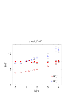
Figure 4: Results for $N_{f}=2$ and $T=2T_{c}$. Left: Distribution of the reweighting factor ($zS_{z}$) for fixed $L$. Right: Screening masses in the channel $0^{+}$ $T=2T_{c}$. ‘Scalar” states (${\rm Tr}A_{0}^{2}$, empty symbols) depend on $\mu/T$, while “gluonic” states (${\rm Tr}F_{12}^{2}$, full symbols ) are practically independent of it. From [11].

As long as $\mu\mathop{\raise 1.29167pt\hbox{$<$\kern-7.5pt\raise-4.73611pt\hbox{$\sim$}}}4T$, the distribution is well contained within $[-\pi,\pi]$ for volumes large enough so that the masses attain their infinite volume values without any cancellations [11]. For even larger values of the chemical potential the sign problem sets in and statistical errors explode.

The results for the lowest screening masses are also displayed in Fig. 4. The different qualitative behaviour of 3d gluonic and scalar states observed generally in scalar gauge models [23, 17, 11] leads to a level crossing at $\mu/T\sim 4.0$ and hence to a change in the nature of the ground state excitation. Hence there is interesting structure in the phase diagram even away from a phase transition, implying that the longest correlation length in the thermal system does not get arbitrarily short with increasing density, but stays at a constant level.

4.2 Imaginary vs. real chemical potential

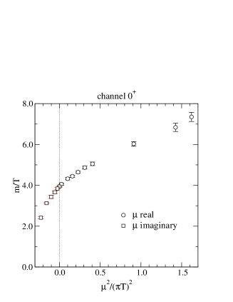
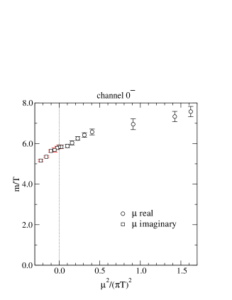
Figure 5: The lowest screening masses at imaginary and real $\mu$, $T=2T_{c}$. From [24].

With an effective theory permitting simulation of real and imaginary chemical potential at hand, one may now return to the suggestion of Sec. 3 and study the feasibility of analytic continuation of observables [24]. Away from phase transitions, the screening masses are analytic in $\mu/T$, as there are no massless modes in the theory. Moreover, since a change $\mu\rightarrow-\mu$ can be compensated for by a field redefinition $A_{0}\rightarrow-A_{0}$ in Eq. (7), all physical observables must be even under this operation. In the 4d theory the same statement follows from compensating $\mu\to-\mu$ by a C (or CP) operation. For small $\mu/T$, the screening masses may thus be written as

$$\frac{M}{T}=c_{0}+c_{1}\biggl{(}\frac{\mu}{\pi T}\biggr{)}^{2}+c_{2}\biggl{(}\frac{\mu}{\pi T}\biggr{)}^{4}\\ +{\cal O}\left(\frac{\mu}{\pi T}\right)^{6}.$$

In the range where this ansatz fits the data of real and imaginary $\mu$, the possibility of analytic continuation is easily checked by examining whether the $c_{i}$ agree between the two data sets.

Fig. 5 shows the lowest states in the system for real and imaginary potential. Note that in the imaginary $\mu$ case, data are only available up to $|\mu|/T\sim 1.5$, and hence $c_{2}$ is not well constrained. The reason is that imaginary chemical potentials favour a $Z_{N}$-broken minimum over the symmetric one in the 4d effective $A_{0}$ potential, once $|\mu|/T\geq\pi/3$. Thus a phase transition occurs and analyticity is lost [7].

In the region up to this critical value, however, one observes firstly that the coefficients $c_{0,1}$ are sufficient to fit the data, and secondly that they are completely compatible between the real and imaginary $\mu$ data sets [24]. Having only two coefficients is equivalent to susceptibility measurements at $\mu=0$. The first conclusion then endorses work based on that latter approach [25]. The second conclusion encourages us to consider 4d QCD at imaginary $\mu$ and study the vicinity of the critical line.

5 QCD at imaginary chemical potential

From the fact that screening masses decrease with imaginary $\mu$ it follows that $T_{c}(Im(\mu))$ is an increasing function, leading to Fig. 6 (left) as the complex generalization of the phase diagram Fig. 1.

Figure 6: Left: Qualitative phase diagram for complex $\mu$. Right: Susceptibility of the Polyakov loop for imaginary $\mu$. $T$ increases with $\beta$.

First results of simulating two-flavour QCD with staggered fermions at imaginary $\mu$ [26] fully confirm this picture, as shown in Fig. 6 (right). The peak of the susceptibility of a gauge invariant operator occurs at a (pseudo-)critical point. The figure clearly shows that the critical coupling $\beta_{c}$ (and with it $T_{c}$) is growing with $|\mu|$. Furthermore, on finite volumes susceptibilities are analytic funtions. This means that $T_{c}(\mu)$ itself is analytic and it might be possible to continue it from imaginary to real $\mu$. This question is currently under investigation.

6 Conclusions

Recent developments have shown that at high temperature, despite the sign problem, lattice simulations can be extended away from the temperature axis into the finite density plane. Considering dimensionally reduced QCD gives a detailed picture of screening masses in the deconfined phase, covering the experimentally relevant parameter space. Furthermore, it establishes that observables depend only weakly on $\mu$ and hence susceptibility measurements as well as analytic continuation from imaginary to real $\mu$ are possible. Multidimensional reweighting has even produced a result for the critical line of the deconfinement transition and its endpoint. Because it uses reweighting, however, an independent check would be desirable.

References

- [1] K. Rajagopal, Nucl. Phys. A 661 (1999) 150
- [2] O. Philipsen, Nucl. Phys. Proc. Suppl. 94 (2001) 49.
- [3] I. M. Barbour et al., Nucl. Phys. Proc. Suppl. 60A (1998) 220.
- [4] I. Barbour et al., Nucl. Phys. B275, 296 (1986); M. A. Stephanov, Phys. Rev. Lett. 76 (1996) 4472.
- [5] A. Vladikas, Nucl. Phys. B (Proc. Suppl.) 4 (1988) 322; D. Toussaint, Nucl. Phys. Proc. Suppl. 17 (1990) 248.
- [6] Z. Fodor and S. D. Katz, hep-lat/0104001; Z. Fodor and S. D. Katz, hep-lat/0106002.
- [7] A. Roberge and N. Weiss, Nucl. Phys. B 275 (1986) 734.
- [8] D. E. Miller and K. Redlich, Phys. Rev. D35 (1987) 2524; A. Hasenfratz and D. Toussaint, Nucl. Phys. B371 (1992) 539.
- [9] M. Alford, A. Kapustin and F. Wilczek, Phys. Rev. D 59 (1999) 054502.
- [10] M.-P. Lombardo, Nucl. Phys. B (Proc. Suppl.) (2000) 83.
- [11] A. Hart, M. Laine and O. Philipsen, Nucl. Phys. B 586 (2000) 443.
- [12] J. Cleymans and K. Redlich, Phys. Rev. C 60 (1999) 054908.
- [13] P. Ginsparg, Nucl. Phys. B170 (1980) 388; T. Appelquist and R. D. Pisarski, Phys. Rev. D23 (1981) 2305.
- [14] S. Nadkarni, Phys. Rev. Lett. 60 (1988) 491; T. Reisz, Z. Phys. C 53 (1992) 169; L. Kärkkäinen et al., Phys. Lett. B 282 (1992) 121; Nucl. Phys. B 418 (1994) 3; Nucl. Phys. B 395 (1993) 733.
- [15] K. Kajantie et al., Nucl. Phys. B503 (1997) 357.
- [16] S. Datta and S. Gupta, Phys. Lett. B471 (2000) 382; Nucl. Phys. B534 (1998) 392.
- [17] A. Hart and O. Philipsen, Nucl. Phys. B572 (2000) 243.
- [18] G. S. Bali et al., Phys. Rev. Lett. 71 (1993) 3059; F. Karsch, E. Laermann and M. Lutgemeier, Phys. Lett. B346 (1995) 94.
- [19] M. Laine and O. Philipsen, Nucl. Phys. B 523 (1998) 267; Phys. Lett. B 459 (1999) 259.
- [20] A. Cucchieri, F. Karsch and P. Petreczky, Phys. Rev. D 64 (2001) 036001.
- [21] P. Bialas et al., Nucl. Phys. B 581 (2000) 477.
- [22] R. V. Gavai and S. Gupta, Phys. Rev. Lett. 85 (2000) 2068.
- [23] O. Philipsen, M. Teper and H. Wittig, Nucl. Phys. B 469 (1996) 445; Nucl. Phys. B 528 (1998) 379.
- [24] A. Hart, M. Laine and O. Philipsen, Phys. Lett. B 505 (2001) 141.
- [25] S. Gottlieb et al., Phys. Rev. D 38 (1988) 2888; C. Bernard et al., Phys. Rev. D 54 (1996) 4585; S. Choe et al. [QCD-TARO Collaboration], hep-lat/0107002.
- [26] Ph. de Forcrand and O. Philipsen, in preparation.