UCCHEP/17–01

IFUSP–1526

Anomaly Mediated Supersymmetry Breaking without $\boldmath{R}$–Parity

F. de Campos¹, M. A. Díaz², O. J. P. Éboli³, M. B. Magro³, and P. G. Mercadante³

¹ Departamento de Física e Química, Universidade Estadual Paulista,
Av. Dr. Ariberto Pereira da Cunha 333, Guaratinguetá, SP, Brazil
² Departamento de Física, Universidad Católica de Chile,
Av. Vicuña Mackenna 4860, Santiago, Chile
³ Instituto de Física, Universidade de São Paulo, CP 66.318,
05389–970, São Paulo, SP, Brazil

Abstract

We analyze the low energy features of a supersymmetric standard model where the anomaly–induced contributions to the soft parameters are dominant in a scenario with bilinear $R$–parity violation. This class of models leads to mixings between the standard model particles and supersymmetric ones which change the low energy phenomenology and searches for supersymmetry. In addition, $R$–parity violation interactions give rise to small neutrino masses which we show to be consistent with the present observations.

1 Introduction

Supersymmetry (SUSY) is a promising candidate for physics beyond the Standard Model (SM) and there is a large ongoing search for supersymmetric partners of the SM particles. However, no positive signal has been observed so far. Therefore, if supersymmetry is a symmetry of nature, it is an experimental fact that it must be broken. The two best known classes of models for supersymmetry breaking are gravity–mediated [1] and gauge–mediated [2] SUSY breaking. In gravity–mediated models, SUSY is assumed to be broken in a hidden sector by fields which interact with the visible particles only via gravitational interactions and not via gauge or Yukawa interactions. In gauge–mediated models, on the contrary, SUSY is broken in a hidden sector and transmitted to the visible sector via SM gauge interactions of messenger particles.

There is a third scenario, called anomaly–mediated SUSY breaking [3], which is based on the observation that the super–Weyl anomaly gives rise to loop contribution to sparticle masses. The anomaly contributions are always present and in some cases they can dominate; this is the anomaly mediated supersymmetry breaking (AMSB) scenario. In this way, the gaugino masses are proportional to their corresponding gauge group $\beta$–functions with the lightest SUSY particle being mainly wino. Analogously, the scalar masses and trilinear couplings are functions of gauge and Yukawa $\beta$–functions. Without further contributions the slepton squared masses turn out to be negative. This tachyonic spectrum is usually cured by adding an universal non–anomaly mediated contribution $m_{0}^{2}>0$ to every scalar mass [4].

So far, most of the work on AMSB has been done assuming $R$–Parity ($R_{P}$) conservation [5, 6, 7]; see [8] for an exception. $R$–Parity violation [9] has received quite some attention lately motivated by the SuperKamiokande collaboration results on neutrino oscillations [10], which indicate neutrinos have mass [11]. One way of introducing mass to the neutrinos is via Bilinear $R$–Parity Violation (BRpV) [12], which is a simple and predictive model for the neutrino masses and mixing angles [13, 14]. In this work, we study the phenomenology of an anomaly mediated SUSY breaking model which includes Bilinear $R$–Parity Violation (AMSB–BRpV), stressing its differences to the $R$–Parity conserving case.

In BRpV–MSSM [15], bilinear $R$–parity and lepton number violating terms are introduced explicitly in the superpotential. These terms induce vacuum expectation values (vev’s) $v_{i}$ for the sneutrinos, and neutrino masses through mixing with neutralinos. At tree level, only one neutrino acquires a mass [16], which is proportional to the sneutrino vev in a basis where the bilinear $R$–Parity violating terms are removed from the superpotential. At one–loop, three neutrinos get a non–zero mass, producing a hierarchical neutrino mass spectrum [17]. It has been shown that the atmospheric mass scale, given by the heaviest neutrino mass, is determined by tree level physics and that the solar mass scale, given by the second heaviest neutrino mass, is determined by one–loop corrections [14].

In our model, the presence of $R_{P}$ violating interactions gives rise to neutrino masses which we show to be consistent with the present observations. Moreover, the low–energy phenomenology is quite distinct of the conserving $R$–Parity AMSB scenario. For instance, the lightest supersymmetric particle (LSP) is unstable, which allows regions of the parameter space where the stau or the tau–sneutrino is the LSP. In our scenario, decays can proceed via the mixing between the standard model particles and supersymmetric ones. As an example, the mixing between the lightest neutralino $\tilde{\chi}^{0}_{1}$ (chargino $\tilde{\chi}^{\pm}_{1}$) and $\nu_{\tau}$ ($\tau^{\pm}$) allows the following decays

$$\tilde{\chi}^{0}_{1} \to\nu_{\tau}Z^{*}\;,$$

$$\tilde{\chi}^{0}_{1} \to\tau^{\pm}W^{\mp*}\;,$$

$$\tilde{\chi}^{\pm}_{1} \to\tau^{\pm}Z^{*}\;,$$

$$\tilde{\chi}^{\pm}_{1} \to\nu_{\tau}W^{\pm*}\;.$$

Another effect of the mixing between the standard model and supersymmetric particles is a sizeable change in the mass of the supersymmetric particles. For instance, the mixing between scalar taus and the charged Higgs can lead to an increase in the splitting between the two scalar tau mass eigenstates by a factor that can be as large as 10 with respect to the $R_{P}$ conserving case.

This paper is organized as follows. We define in Sec. 2 our anomaly mediated SUSY breaking model which includes Bilinear $R$–Parity Violation, stating explicitly our working hypotheses. This Section also contains an overall view of the supersymmetric spectrum in our model. We study the properties of the CP–odd, CP–even, and charged scalar particles in Sections 3, 4, and 5 respectively, concentrating on the mixing angles that arise from the introduction of the $R$–Parity violating terms. Section 6 contains the analysis that shows that our model can generate neutrino masses in agreement with the present knowledge. In Sec. 7 we provide a discussion of the general phenomenological aspects of our model while in Sec. 8 we draw our conclusions.

2 The AMSB–BRpV model

Our model, besides the usual $R_{P}$ conserving Yukawa terms in the superpotential, includes the following bilinear terms

$$W_{bilinear}=-\varepsilon_{ab}\left(\mu\widehat{H}_{d}^{a}\widehat{H}_{u}^{b}+\epsilon_{i}\widehat{L}_{i}^{a}\widehat{H}_{u}^{b}\right)\;,$$ (1)

where the second one violates $R_{P}$ and we take $|\epsilon_{i}|\ll|\mu|$. Analogously, the relevant soft bilinear terms are

$$V_{soft} = m_{H_{u}}^{2}H_{u}^{a*}H_{u}^{a}+m_{H_{d}}^{2}H_{d}^{a*}H_{d}^{a}+M_{L_{i}}^{2}\widetilde{L}_{i}^{a*}\widetilde{L}_{i}^{a}-$$ (2)

$$-\varepsilon_{ab}\left(B\mu H_{d}^{a}H_{u}^{b}+B_{i}\epsilon_{i}\widetilde{L}_{i}^{a}H_{u}^{b}\right)\;,$$

where the terms proportional to $B_{i}$ are the ones that violates $R_{P}$. The explicit $R_{P}$ violating terms induce vacuum expectation values $v_{i}$, $i=1,2,3$ for the sneutrinos, in addition to the two Higgs doublets vev’s $v_{u}$ and $v_{d}$. In phenomenological studies where the details of the neutrino sector are not relevant, it has been proven very useful to work in the approximation where $R_{P}$ and lepton number are violated in only one generation [18]. In these cases, a determination of the mass scale of the atmospheric neutrino anomaly within a factor of two is usually enough, and that can be achieved in the approximation where $R_{P}$ is violated only in the third generation.

In this work we assume that $R_{P}$ violation takes place only in the third generation, and consequently the parameter space of our model is

$$m_{0}\,,\,m_{3/2}\,,\,\tan\beta\,,\,{\mathrm{sign}}(\mu)\,,\,\epsilon_{3}\,,\,{\mathrm{and}}\,\,m_{\nu_{\tau}}\,,$$ (3)

where $m_{3/2}$ is the gravitino mass and $m_{0}^{2}$ is the non–anomaly mediated contribution to the soft masses needed to avoid the appearance of tachyons. We characterize the BRpV sector by the $\epsilon_{3}$ term in the superpotential and the tau–neutrino mass $m_{\nu_{\tau}}$ since it is convenient to trade $v_{3}$ by $m_{\nu_{\tau}}$.

In AMSB models, the soft terms are fixed in a non–universal way at the unification scale which we assumed to be $M_{GUT}=2.4\times 10^{16}$ GeV; see Appendix A for details. We considered the running of the masses and couplings to the electroweak scale, assumed to be the top mass, using the one–loop renormalization group equations (RGE) that are presented in Appendix B. In the evaluation of the gaugino masses, we included the next–to–leading order (NLO) corrections coming from $\alpha_{s}$, the two–loop top Yukawa contributions to the beta–functions, and threshold corrections enhanced by large logarithms; for details see [4]. The NLO corrections are especially important for $M_{2}$, leading to a change in the wino mass by more than 20%.

One of the virtues of AMSB models is that the $SU(2)\otimes U(1)$ symmetry is broken radiatively by the running of the RGE from the GUT scale to the weak one. This feature is preserved by our model since the one–loop RGE are not affected by the bilinear $R_{P}$ violating interactions; see Appendix B. In our model, the electroweak symmetry is broken by the vacuum expectation values of the two Higgs doublets $H_{d}$ and $H_{u}$, and the neutral component of the third left slepton doublet $\widetilde{L}_{3}$. We denote these fields as

$$H_{d}={{{1\over{\sqrt{2}}}[\chi^{0}_{d}+v_{d}+i\varphi^{0}_{d}]}\choose{H^{-}_{d}}}\,,\qquad H_{u}={{H^{+}_{u}}\choose{{1\over{\sqrt{2}}}[\chi^{0}_{u}+v_{u}+i\varphi^{0}_{u}]}}\,,$$

$$\qquad\qquad\qquad\widetilde{L}_{3}={{{1\over{\sqrt{2}}}[\tilde{\nu}^{R}_{\tau}+v_{3}+i\tilde{\nu}^{i0}_{\tau}]}\choose{\tilde{\tau}^{-}}}\,.$$ (4)

The above vev’s $v_{i}$ can be obtained through the minimization conditions, or tadpole equations, which in the AMSB–BRpV model are

$$t_{d}^{0} = (m_{H_{d}}^{2}+\mu^{2})v_{d}-B\mu v_{u}-\mu\epsilon_{3}v_{3}+{\textstyle{1\over 8}}(g^{2}+g^{\prime 2})v_{d}(v_{d}^{2}-v_{u}^{2}+v_{3}^{2})\,,$$

$$t_{u}^{0} = (m_{H_{u}}^{2}+\mu^{2}+\epsilon_{3}^{2})v_{u}-B\mu v_{d}+B_{3}\epsilon_{3}v_{3}-{\textstyle{1\over 8}}(g^{2}+g^{\prime 2})v_{u}(v_{d}^{2}-v_{u}^{2}+v_{3}^{2})\,,$$

$$t_{3}^{0} = (m_{L_{3}}^{2}+\epsilon_{3}^{2})v_{3}-\mu\epsilon_{3}v_{d}+B_{3}\epsilon_{3}v_{u}+{\textstyle{1\over 8}}(g^{2}+g^{\prime 2})v_{3}(v_{d}^{2}-v_{u}^{2}+v_{3}^{2})\,,$$ (5)

at tree level. At the minimum we must impose $t^{0}_{d}=t^{0}_{u}=t^{0}_{3}=0$. In practice, the input parameters are the soft masses $m_{H_{d}}$, $m_{H_{u}}$, and $m_{L_{3}}$, the vev’s $v_{u}$, $v_{d}$, and $v_{3}$ (obtained from $m_{Z}$, $\tan\beta$, and $m_{\nu_{\tau}}$), and $\epsilon_{3}$. We then use the tadpole equations to determine $B$, $B_{3}$, and $|\mu|$.

One–loop corrections to the tadpole equations change the value of $|\mu|$ by ${\cal O}(20\%)$, therefore, we also included the one–loop corrections due to third generation of quarks and squarks [17]:

$$t_{i}=t_{i}^{0}+\tilde{T}_{i}(Q)\;,$$ (6)

where $t_{i}$, with $i=d,u$, are the renormalized tadpoles, $t_{i}^{0}$ are given in (5), and $\tilde{T}_{i}(Q)$ are the renormalized one–loop contributions at the scale $Q$. Here we neglected the one–loop corrections for $t_{3}$ since we are only interested in the value of $\mu$.

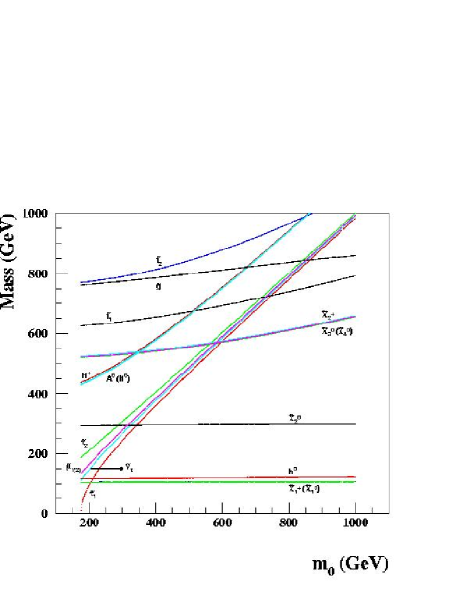
Figure 1: Supersymmetric mass spectrum in AMSB–BRpV for $m_{3/2}=32$ TeV, $\tan\beta=5$, and $\mu<0$. The values of $\epsilon_{3}$ and $m_{\nu_{\tau}}$ were randomly varied according to $10^{-5}<\epsilon_{3}<1$ GeV and $10^{-6}<m_{\nu_{\tau}}<1$ eV.

Using the procedure underlined above, the whole mass spectrum can be calculated as a function of the input parameters $m_{0}$, $m_{3/2}$, $\tan\beta$, ${\mathrm{sign}}(\mu)$, $\epsilon_{3}$, and $m_{\nu_{\tau}}$. In Fig. 1, we show a scatter plot of the mass spectrum as a function of the scalar mass $m_{0}$ for $m_{3/2}=32$ TeV, $\tan\beta=5$, and $\mu<0$, varying $\epsilon_{3}$ and $m_{\nu_{\tau}}$ according to $10^{-5}<\epsilon_{3}<1$ GeV and $10^{-6}<m_{\nu_{\tau}}<1$ eV. The widths of the scatter plots show that the spectrum exhibits a very small dependence on $\epsilon_{3}$ and $m_{\nu_{\tau}}$. Throughout this paper we use this range for $\epsilon_{3}$ and $m_{\nu_{\tau}}$ in all figures.

We can see from this figure that, for $m_{0}\mathrel{\vbox{\hbox{$>$}\nointerlineskip\hbox{$\sim$}}}200$ GeV, the LSP is the lightest neutralino $\tilde{\chi}^{0}_{1}$ with the lightest chargino $\tilde{\chi}^{+}_{1}$ almost degenerated with it, as in $R_{P}$–conserving AMSB. Nevertheless, the LSP is the lightest stau $\tilde{\tau}_{1}^{+}$ for $m_{0}\mathrel{\vbox{\hbox{$<$}\nointerlineskip\hbox{$\sim$}}}200$ GeV. This last region of parameter space is forbidden in $R_{P}$–conserving AMSB, but perfectly possible in AMSB–BRpV since the stau is unstable, decaying into $R_{P}$–violating modes with sizeable branching ratios. Furthermore, the slepton masses have a strong dependence on $m_{0}$. We plotted masses of the two staus, which have an appreciable splitting, the almost degenerated smuons, and the closely degenerated tau–sneutrinos. The heavy Higgs bosons have also a strong dependence on $m_{0}$ and, for the chosen parameters, they are much heavier than the sleptons. On the other hand, the gauginos show little dependence on $m_{0}$, as expected.

3 CP–odd Higgs/Sneutrino Sector

In our model, the CP–odd Higgs sector mixes with the imaginary part of the tau–sneutrino due to the bilinear $R_{P}$ violating interactions. Writing the mass terms in the form

$$V_{quadratic}={\textstyle{1\over 2}}[\varphi^{0}_{d},\varphi^{0}_{u},\tilde{\nu}_{\tau}^{i0}]{\kern-0.24994pt\hbox{$M$}\kern-10.79166pt\kern 0.50003pt\hbox{$M$}\kern-10.79166pt\kern-0.24994pt\raise 0.43304pt\hbox{$M$}^{2}_{P^{0}}}\left[\matrix{\varphi^{0}_{d}\cr\varphi^{0}_{u}\cr\tilde{\nu}_{\tau}^{i0}}\right]\;,$$ (7)

we have

$${\scriptsize{\kern-0.17496pt\hbox{$M$}\kern-7.55415pt\kern 0.35002pt\hbox{$M$}\kern-7.55415pt\kern-0.17496pt\raise 0.30313pt\hbox{$M$}_{P^{0}}^{2}}=\left[\matrix{m_{A}^{2(0)}s_{\beta}^{2}+\mu\epsilon_{3}{{v_{3}}\over{v_{d}}}&m_{A}^{2(0)}s_{\beta}c_{\beta}&-\mu\epsilon_{3}\cr m_{A}^{2(0)}s_{\beta}c_{\beta}&m_{A}^{2(0)}c_{\beta}^{2}-\mu\epsilon_{3}{{v_{3}}\over{v_{d}}}{{c_{\beta}^{2}}\over{s_{\beta}^{2}}}+{{v_{3}^{2}}\over{v_{d}^{2}}}{{c_{\beta}^{2}}\over{s_{\beta}^{2}}}\overline{m}_{\tilde{\nu}_{\tau}}^{2}&-\mu\epsilon_{3}{{c_{\beta}}\over{s_{\beta}}}+{{v_{3}}\over{v_{d}}}{{c_{\beta}}\over{s_{\beta}}}\overline{m}_{\tilde{\nu}_{\tau}}^{2}\cr-\mu\epsilon_{3}&-\mu\epsilon_{3}{{c_{\beta}}\over{s_{\beta}}}+{{v_{3}}\over{v_{d}}}{{c_{\beta}}\over{s_{\beta}}}\overline{m}_{\tilde{\nu}_{\tau}}^{2}&\overline{m}_{\tilde{\nu}_{\tau}}^{2}}\right]\;,}$$ (8)

with $\overline{m}_{\tilde{\nu}_{\tau}}^{2}=m_{\tilde{\nu}_{\tau}}^{2(0)}+\epsilon_{3}^{2}+{\textstyle{1\over 8}}g_{Z}^{2}v_{3}^{2}$ and $g_{Z}^{2}\equiv g^{2}+g^{\prime 2}$. Here,

$$m_{A}^{2(0)}={{B\mu}\over{s_{\beta}c_{\beta}}}\qquad\hbox{and}\qquad m_{\tilde{\nu}_{\tau}}^{2(0)}=M_{L_{3}}^{2}+{\textstyle{1\over 8}}g_{Z}^{2}(v_{d}^{2}-v_{u}^{2})$$ (9)

are respectively the CP–odd Higgs and sneutrino masses in the $R_{P}$ conserving limit ($\epsilon_{3}=v_{3}=0$). In order to write this mass matrix we have eliminated $m_{H_{u}}^{2}$, $m_{H_{d}}^{2}$, and $B_{3}$ using the tadpole equations (5). The mass matrix has an explicitly vanishing eigenvalue, which corresponds to the neutral Goldstone boson.

This matrix can be diagonalized with a rotation

$$\left[\matrix{A^{0}\cr G^{0}\cr\tilde{\nu}_{\tau}^{odd}}\right]={\kern-0.24994pt\hbox{$R$}\kern-7.67015pt\kern 0.50003pt\hbox{$R$}\kern-7.67015pt\kern-0.24994pt\raise 0.43304pt\hbox{$R$}_{P^{0}}}\left[\matrix{\varphi^{0}_{d}\cr\varphi^{0}_{u}\cr\tilde{\nu}_{\tau}^{i0}}\right]\;,$$ (10)

where $G^{0}$ is the massless neutral Goldstone boson. Between the other two eigenstates, the one with largest $\tilde{\nu}_{\tau}^{i0}$ component is called CP–odd tau–sneutrino $\tilde{\nu}_{\tau}^{odd}$ and the remaining state is called CP–odd Higgs $A^{0}$.

As an intermediate step, it is convenient to make explicit the masslessness of the Goldstone boson with the rotation

$${\kern-0.24994pt\hbox{$\widehat{R}_{P^{0}}$}\kern-11.52863pt\kern 0.50003pt\hbox{$\widehat{R}_{P^{0}}$}\kern-11.52863pt\kern-0.24994pt\raise 0.43304pt\hbox{$\widehat{R}_{P^{0}}$}}=\left[\matrix{s_{\beta}&c_{\beta}&0\cr-c_{\beta}r&s_{\beta}r&-{{v_{3}}\over{v_{d}}}c_{\beta}r\cr-{{v_{3}}\over{v_{d}}}c_{\beta}^{2}r&{{v_{3}}\over{v_{d}}}s_{\beta}c_{\beta}r&r}\right]\;,$$ (11)

where

$$r={1\over{\sqrt{1+{{v_{3}^{2}}\over{v_{d}^{2}}}c_{\beta}^{2}}}}\;,$$ (12)

obtaining a rotated mass matrix $\widehat{R}_{P^{0}}M_{P^{0}}^{2}\widehat{R}_{P^{0}}^{T}$ which has a column and a row of zeros, corresponding to $G^{0}$. This procedure simplifies the analysis since the remaining $2\times 2$ mass matrix for $(A^{0},\tilde{\nu}_{\tau}^{odd})$ is

$${\kern-0.24994pt\hbox{$\widehat{M}$}\kern-5.55557pt\kern 0.50003pt\hbox{$\widehat{M}$}\kern-5.55557pt\kern-0.24994pt\raise 0.43304pt\hbox{$\widehat{M}$}}^{2}_{P^{0}}=\left[\matrix{m_{A}^{2(0)}+{{v_{3}^{2}}\over{v_{d}^{2}}}{{c_{\beta}^{4}}\over{s_{\beta}^{2}}}\overline{m}_{\tilde{\nu}_{\tau}}^{2}+\mu\epsilon_{3}{{v_{3}}\over{v_{d}}}{{s_{\beta}^{2}-c_{\beta}^{2}}\over{s_{\beta}^{2}}}&\left({{v_{3}}\over{v_{d}}}{{c_{\beta}^{2}}\over{s_{\beta}}}\overline{m}_{\tilde{\nu}_{\tau}}^{2}-\mu\epsilon_{3}{1\over{s_{\beta}}}\right)r\cr\left({{v_{3}}\over{v_{d}}}{{c_{\beta}^{2}}\over{s_{\beta}}}\overline{m}_{\tilde{\nu}_{\tau}}^{2}-\mu\epsilon_{3}{1\over{s_{\beta}}}\right)r&\overline{m}_{\tilde{\nu}_{\tau}}^{2}{1\over r^{2}}}\right]\;.$$ (13)

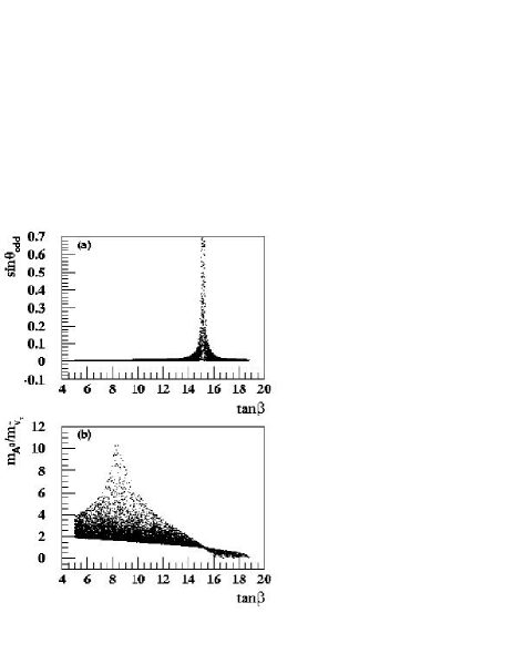
Figure 2: (a) CP–odd Higgs–sneutrino mixing and (b) ratio between the CP–odd Higgs mass and the sneutrino mass as a function of $\tan\beta$ for $m_{3/2}=32$ TeV, $\mu<0$ and $100<m_{0}<300$ GeV.

We quantify the mixing between the tau–sneutrino and the neutral Higgs bosons through

$$\sin^{2}{\theta_{odd}}=|\langle\tilde{\nu}_{\tau}^{odd}|\varphi^{0}_{u}\rangle|^{2}+|\langle\tilde{\nu}_{\tau}^{odd}|\varphi^{0}_{d}\rangle|^{2}\;.$$ (14)

If we consider the $R_{P}$ violating interactions as a perturbation, we can show that

$$\sin^{2}{\theta_{odd}}\simeq{{\left({{v_{3}}\over{v_{d}}}c_{\beta}^{2}m_{\tilde{\nu}_{\tau}}^{2(0)}-\mu\epsilon_{3}\right)^{2}}\over{s_{\beta}^{2}\left(m_{A}^{2(0)}-m_{\tilde{\nu}_{\tau}}^{2(0)}\right)^{2}}}+\frac{v_{3}^{2}}{v_{d}^{2}}c^{2}_{\beta}\;,$$ (15)

indicating that this mixing can be large when the CP–odd Higgs boson $A^{0}$ and the sneutrino $\tilde{\nu}_{\tau}$ are approximately degenerate.

Figure 2a displays the full sneutrino–Higgs mixing (14), with no approximations, as a function of $\tan\beta$ for $m_{3/2}=32$ TeV, $\mu<0$ and $100<m_{0}<300$ GeV. In a large fraction of the parameter space this mixing is small, since it is proportional to the BRpV parameters squared divided by MSSM mass parameters squared. However, it is possible to find a region where the mixing is sizable, e.g., for our choice of parameters this happens at $\tan\beta\approx 15$. As expected, the region of large mixing is associated to near degenerate states, as we can see from Fig. 2b where we present the ratio between the CP–odd Higgs mass $m_{A}$ and the CP–odd tau–sneutrino mass $m_{\tilde{\nu}_{\tau}^{odd}}$ as a function of $\tan\beta$.

4 CP–even Higgs/Sneutrino Sector

The mass terms of the CP–even neutral scalar sector are

$$V_{quadratic}={\textstyle{1\over 2}}[\chi^{0}_{d},\chi^{0}_{u},\tilde{\nu}_{\tau}^{r0}]{\kern-0.24994pt\hbox{$M$}\kern-10.79166pt\kern 0.50003pt\hbox{$M$}\kern-10.79166pt\kern-0.24994pt\raise 0.43304pt\hbox{$M$}^{2}_{S^{0}}}\left[\matrix{\chi^{0}_{d}\cr\chi^{0}_{u}\cr\tilde{\nu}_{\tau}^{r0}}\right]\;,$$ (16)

where the mass matrix can be separated into two pieces

$${\kern-0.24994pt\hbox{$M$}\kern-10.79166pt\kern 0.50003pt\hbox{$M$}\kern-10.79166pt\kern-0.24994pt\raise 0.43304pt\hbox{$M$}^{2}_{S^{0}}}={\kern-0.24994pt\hbox{$M$}\kern-10.79166pt\kern 0.50003pt\hbox{$M$}\kern-10.79166pt\kern-0.24994pt\raise 0.43304pt\hbox{$M$}_{S^{0}}^{2(0)}}+{\kern-0.24994pt\hbox{$M$}\kern-10.79166pt\kern 0.50003pt\hbox{$M$}\kern-10.79166pt\kern-0.24994pt\raise 0.43304pt\hbox{$M$}_{S^{0}}^{2(1)}}\;.$$ (17)

The first term due to $R_{P}$ conserving interactions is

$${\kern-0.24994pt\hbox{$M$}\kern-10.79166pt\kern 0.50003pt\hbox{$M$}\kern-10.79166pt\kern-0.24994pt\raise 0.43304pt\hbox{$M$}_{S^{0}}^{2(0)}}=\left[\matrix{m_{A}^{2(0)}s_{\beta}^{2}+{\textstyle{1\over 4}}g_{Z}^{2}v_{d}^{2}&-m_{A}^{2(0)}s_{\beta}c_{\beta}-{\textstyle{1\over 4}}g^{2}_{Z}v_{d}v_{u}&0\cr-m_{A}^{2(0)}s_{\beta}c_{\beta}-{\textstyle{1\over 4}}g^{2}_{Z}v_{d}v_{u}&m_{A}^{2(0)}c_{\beta}^{2}+{\textstyle{1\over 4}}g_{Z}^{2}v_{u}^{2}&0\cr 0&0&m_{\tilde{\nu}_{\tau}}^{2(0)}}\right]\;,$$ (18)

while the one associated to the $R_{P}$ violating terms is

$${\scriptsize\!\!{\kern-0.17496pt\hbox{$M$}\kern-7.55415pt\kern 0.35002pt\hbox{$M$}\kern-7.55415pt\kern-0.17496pt\raise 0.30313pt\hbox{$M$}_{S^{0}}^{2(1)}}=\left[\matrix{\mu\epsilon_{3}{{v_{3}}\over{v_{d}}}&0&-\mu\epsilon_{3}+{\textstyle{1\over 4}}g^{2}_{Z}v_{d}v_{3}\cr 0&{{v_{3}^{2}}\over{v_{d}^{2}}}{{c_{\beta}^{2}}\over{s_{\beta}^{2}}}m_{\tilde{\nu}_{\tau}}^{2(0)}-\mu\epsilon_{3}{{v_{3}}\over{v_{d}}}{{c_{\beta}^{2}}\over{s_{\beta}^{2}}}&\mu\epsilon_{3}{{c_{\beta}}\over{s_{\beta}}}-{{v_{3}}\over{v_{d}}}{{c_{\beta}}\over{s_{\beta}}}m_{\tilde{\nu}_{\tau}}^{2(0)}-{\textstyle{1\over 4}}g^{2}_{Z}v_{u}v_{3}\cr-\mu\epsilon_{3}+{\textstyle{1\over 4}}g^{2}_{Z}v_{d}v_{3}&\mu\epsilon_{3}{{c_{\beta}}\over{s_{\beta}}}-{{v_{3}}\over{v_{d}}}{{c_{\beta}}\over{s_{\beta}}}m_{\tilde{\nu}_{\tau}}^{2(0)}-{\textstyle{1\over 4}}g^{2}_{Z}v_{u}v_{3}&\epsilon_{3}^{2}+{\textstyle{3\over 8}}g^{2}_{Z}v_{3}^{2}}\right]\;.}$$ (19)

Radiative corrections can change significantly the lightest Higgs mass and, consequently, we have also introduced the leading correction to its mass

$$\Delta m_{\chi^{0}_{u}}\equiv\frac{3m^{4}_{t}}{2\pi^{2}v_{u}^{2}v^{\prime}}\ln\left(\frac{m_{\tilde{t}_{1}}m_{\tilde{t}_{2}}}{m^{2}_{t}}\right)\;,$$ (20)

with

$$v^{\prime}=1-\frac{v_{3}^{2}}{v_{d}^{2}+v_{u}^{2}+v_{3}^{2}}\;,$$ (21)

by adding it to the element $[{\kern-0.24994pt\hbox{$M$}\kern-10.79166pt\kern 0.50003pt\hbox{$M$}\kern-10.79166pt\kern-0.24994pt\raise 0.43304pt\hbox{$M$}_{S^{0}}^{2}}]_{22}$.

Analogously to the CP–odd sector, we define the mixing between the CP–even tau–sneutrino and the neutral Higgs bosons as

$$\sin^{2}{\theta_{even}}=|\langle\tilde{\nu}_{\tau}^{even}|\chi^{0}_{d}\rangle|^{2}+|\langle\tilde{\nu}_{\tau}^{even}|\chi^{0}_{u}\rangle|^{2}=|\langle H^{0}|\tilde{\nu}_{\tau}^{r0}\rangle|^{2}+|\langle h^{0}|\tilde{\nu}_{\tau}^{r0}\rangle|^{2}\;.$$ (22)

In general, this mixing is small since it is proportional to the $R_{P}$ breaking parameters squared, however, it can be large provided the sneutrino is degenerate either with $h^{0}$ or $H^{0}$.

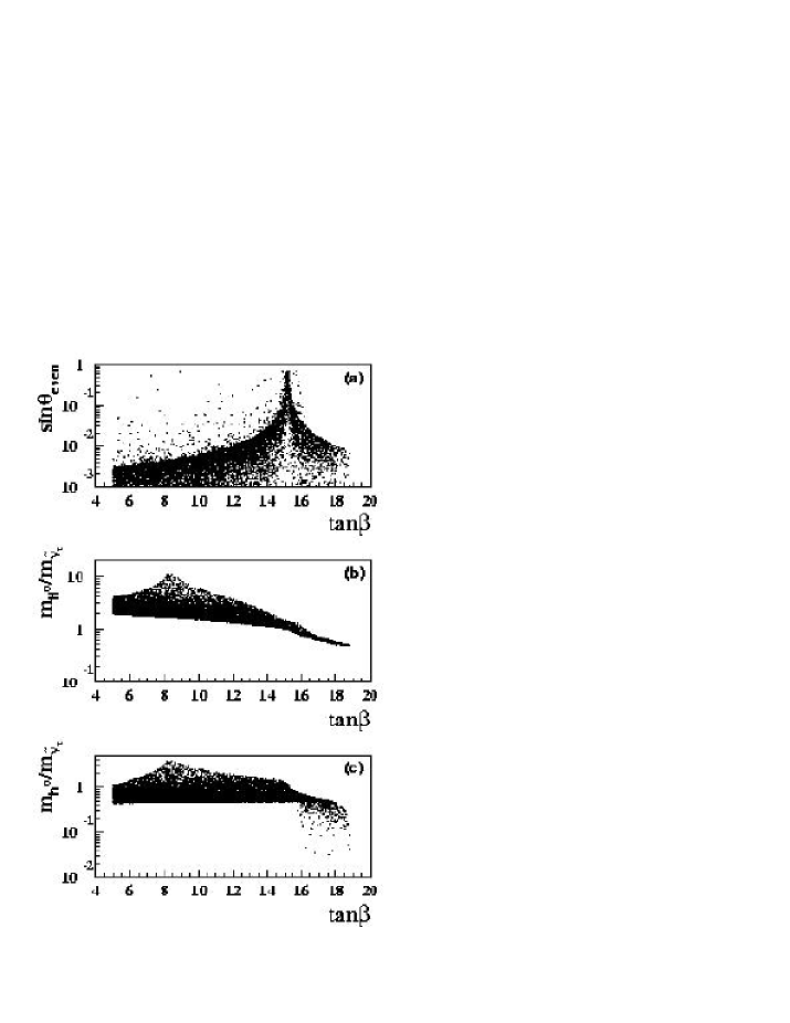
Figure 3: (a) CP–even Higgs–sneutrino mixing; (b) ratio between heavy CP–even Higgs and tau–sneutrino masses and (c) ratio between light CP–even Higgs and tau–sneutrino masses as a function of $\tan\beta$ for $m_{3/2}=32$ TeV, $\mu<0$ and $100<m_{0}<300$ GeV.

In Figure 3a, we present the mixing (22) as a function of $\tan\beta$, for the input parameters as in Fig. 2. Similarly to the CP–odd scalar sector, this mixing can be very large, occurring either when $m_{H}\approx m_{\tilde{\nu}_{\tau}^{even}}$ or $m_{h}\approx m_{\tilde{\nu}_{\tau}^{even}}$. In fact, we can see from Fig. 3b that the peak in Fig. 3a for $\tan\beta\sim 15$ is mainly due to the mass degeneracy between the heavy CP–even Higgs $H^{0}$ and the CP–even tau–sneutrino $\tilde{\nu}_{\tau}^{even}$. On the other hand, the other scattered dots with high mixing angle values throughout Fig. 3a come from points in the parameter space where the light CP–even Higgs $h^{0}$ and the CP–even tau–sneutrino $\tilde{\nu}_{\tau}^{even}$ are degenerated. We see from Fig. 3c that this may occur for $5<\tan\beta<15$.

It is important to notice that the enhancement of the mixing between the tau–sneutrino and the CP–even Higgs bosons for almost degenerate states implies that large $R_{P}$ violating effects are possible even for small $R_{P}$ violating parameters ($\epsilon_{3}\mathrel{\vbox{\hbox{$<$}\nointerlineskip\hbox{$\sim$}}}1$ GeV), and for neutrino masses consistent with the solutions to the atmospheric neutrino anomaly ($m_{\nu_{\tau}}\mathrel{\vbox{\hbox{$<$}\nointerlineskip\hbox{$\sim$}}}1$ eV).

5 Charged Higgs/Charged Slepton Sector

The mass terms in the charged scalar sector are

$$V_{quadratic}=[H_{u}^{-},H_{d}^{-},\tilde{\tau}_{L}^{-},\tilde{\tau}_{R}^{-}]{\kern-0.24994pt\hbox{$M$}\kern-10.79166pt\kern 0.50003pt\hbox{$M$}\kern-10.79166pt\kern-0.24994pt\raise 0.43304pt\hbox{$M$}^{2}_{S^{\pm}}}\left[\matrix{H_{u}^{+}\cr H_{d}^{+}\cr\tilde{\tau}_{L}^{+}\cr\tilde{\tau}_{R}^{+}}\right]\;,$$ (23)

where it is convenient to split the mass matrix into a $R_{P}$ conserving part and a $R_{P}$ violating one.

$${\kern-0.24994pt\hbox{$M$}\kern-10.79166pt\kern 0.50003pt\hbox{$M$}\kern-10.79166pt\kern-0.24994pt\raise 0.43304pt\hbox{$M$}^{2}_{S^{\pm}}}={\kern-0.24994pt\hbox{$M$}\kern-10.79166pt\kern 0.50003pt\hbox{$M$}\kern-10.79166pt\kern-0.24994pt\raise 0.43304pt\hbox{$M$}^{2(0)}_{S^{\pm}}}+{\kern-0.24994pt\hbox{$M$}\kern-10.79166pt\kern 0.50003pt\hbox{$M$}\kern-10.79166pt\kern-0.24994pt\raise 0.43304pt\hbox{$M$}^{2(1)}_{S^{\pm}}}\;.$$ (24)

The $R_{P}$ conserving mass matrix has the usual MSSM form

${\small{\kern-0.22495pt\hbox{$M$}\kern-9.7125pt\kern 0.45003pt\hbox{$M$}\kern-9.7125pt\kern-0.22495pt\raise 0.38974pt\hbox{$M$}^{2(0)}_{S^{\pm}}}=}$

$${\scriptsize=\left[\matrix{m_{A}^{2(0)}s_{\beta}^{2}+{\textstyle{1\over 4}}g^{2}v_{u}^{2}&m_{A}^{2(0)}s_{\beta}c_{\beta}+{\textstyle{1\over 4}}g^{2}v_{u}v_{d}&0&0\cr m_{A}^{2(0)}s_{\beta}c_{\beta}+{\textstyle{1\over 4}}g^{2}v_{u}v_{d}&m_{A}^{2(0)}c_{\beta}^{2}+{\textstyle{1\over 4}}g^{2}v_{d}^{2}&0&0\cr 0&0&\widehat{M}_{L_{3}}^{2}&{1\over{\sqrt{2}}}h_{\tau}(A_{\tau}v_{d}-\mu v_{u})\cr 0&0&{1\over{\sqrt{2}}}h_{\tau}(A_{\tau}v_{d}-\mu v_{u})&\widehat{M}_{R_{3}}^{2}}\right]\;,}$$ (25)

where $h_{\tau}$ is the $\tau$ Yukawa coupling and

$$\widehat{M}_{L_{3}}^{2} = M_{L_{3}}^{2}-{\textstyle{1\over 8}}(g^{2}-g^{\prime 2})(v_{d}^{2}-v_{u}^{2})+{\textstyle{1\over 2}}h_{\tau}^{2}v_{d}^{2}\;,$$

$$\widehat{M}_{R_{3}}^{2} = M_{R_{3}}^{2}-{\textstyle{1\over 4}}g^{\prime 2}(v_{d}^{2}-v_{u}^{2})+{\textstyle{1\over 2}}h_{\tau}^{2}v_{d}^{2}\;.$$ (26)

The contribution due to $R_{P}$ violating terms is

${\small{\kern-0.22495pt\hbox{$M$}\kern-9.7125pt\kern 0.45003pt\hbox{$M$}\kern-9.7125pt\kern-0.22495pt\raise 0.38974pt\hbox{$M$}^{2(1)}_{S^{\pm}}}=}$

$${\scriptsize=\left[\matrix{\mu\epsilon_{3}{{v_{3}}\over{v_{d}}}-{\textstyle{1\over 4}}g^{2}v_{3}^{2}+{\textstyle{1\over 2}}h_{\tau}^{2}v_{3}^{2}&0&X_{uL}&X_{uR}\cr 0&{{v_{3}^{2}}\over{v_{d}^{2}}}{{c_{\beta}^{2}}\over{s_{\beta}^{2}}}\overline{m}_{\tilde{\nu}}^{2}-\mu\epsilon_{3}{{v_{3}}\over{v_{d}}}{{c_{\beta}^{2}}\over{s_{\beta}^{2}}}+{\textstyle{1\over 4}}g^{2}v_{3}^{2}&X_{dL}&X_{dR}\cr X_{uL}&X_{dL}&\epsilon_{3}^{2}+{\textstyle{1\over 8}}g_{Z}^{2}v_{3}^{2}&0\cr X_{uR}&X_{dR}&0&{\textstyle{1\over 2}}h_{\tau}^{2}v_{3}^{2}-{\textstyle{1\over 4}}g^{\prime 2}v_{3}^{2}}\right]\;,}$$ (27)

with

$$X_{uL} = {\textstyle{1\over 4}}g^{2}v_{d}v_{3}-\mu\epsilon_{3}-{\textstyle{1\over 2}}h_{\tau}^{2}v_{d}v_{3}\;,$$ (28)

$$X_{uR} = -{1\over{\sqrt{2}}}h_{\tau}(A_{\tau}v_{3}+\epsilon_{3}v_{u})\;,$$ (29)

$$X_{dL} = {{v_{3}}\over{v_{d}}}{{c_{\beta}}\over{s_{\beta}}}\overline{m}_{\tilde{\nu}}^{2}-\mu\epsilon_{3}{{c_{\beta}}\over{s_{\beta}}}+{\textstyle{1\over 4}}g^{2}v_{u}v_{3}\;,$$ (30)

$$X_{dR} = -{1\over{\sqrt{2}}}h_{\tau}(\mu v_{3}+\epsilon_{3}v_{d})\;.$$ (31)

The complete matrix ${\kern-0.24994pt\hbox{$M$}\kern-10.79166pt\kern 0.50003pt\hbox{$M$}\kern-10.79166pt\kern-0.24994pt\raise 0.43304pt\hbox{$M$}^{2}_{S^{\pm}}}$ has an explicit zero eigenvalue corresponding to the charged Goldstone boson $G^{\pm}$, and is diagonalized by a rotation matrix ${\kern-0.24994pt\hbox{$R$}\kern-7.67015pt\kern 0.50003pt\hbox{$R$}\kern-7.67015pt\kern-0.24994pt\raise 0.43304pt\hbox{$R$}_{S^{\pm}}}$ such that

$$\left[\matrix{H^{+}\cr G^{+}\cr\tilde{\tau}_{1}^{+}\cr\tilde{\tau}_{2}^{+}}\right]={\kern-0.24994pt\hbox{$R$}\kern-7.67015pt\kern 0.50003pt\hbox{$R$}\kern-7.67015pt\kern-0.24994pt\raise 0.43304pt\hbox{$R$}_{S^{\pm}}}\left[\matrix{H_{u}^{+}\cr H_{d}^{+}\cr\tilde{\tau}_{L}^{+}\cr\tilde{\tau}_{R}^{+}}\right]\;.$$ (32)

In analogy with the discussion on the CP–even scalar sector, we define the mixing of the lightest (heaviest) stau $\tilde{\tau}_{1}^{\pm}$ ($\tilde{\tau}_{2}^{\pm}$) with the charged Higgs bosons as

$$\sin^{2}{\theta^{+}_{1}} = |\langle\tilde{\tau}_{1}^{+}|H^{+}_{u}\rangle|^{2}+|\langle\tilde{\tau}_{1}^{+}|H^{+}_{d}\rangle|^{2}\;,$$ (33)

$$\sin^{2}{\theta^{+}_{2}} = |\langle\tilde{\tau}_{2}^{+}|H^{+}_{u}\rangle|^{2}+|\langle\tilde{\tau}_{2}^{+}|H^{+}_{d}\rangle|^{2}\;.$$ (34)

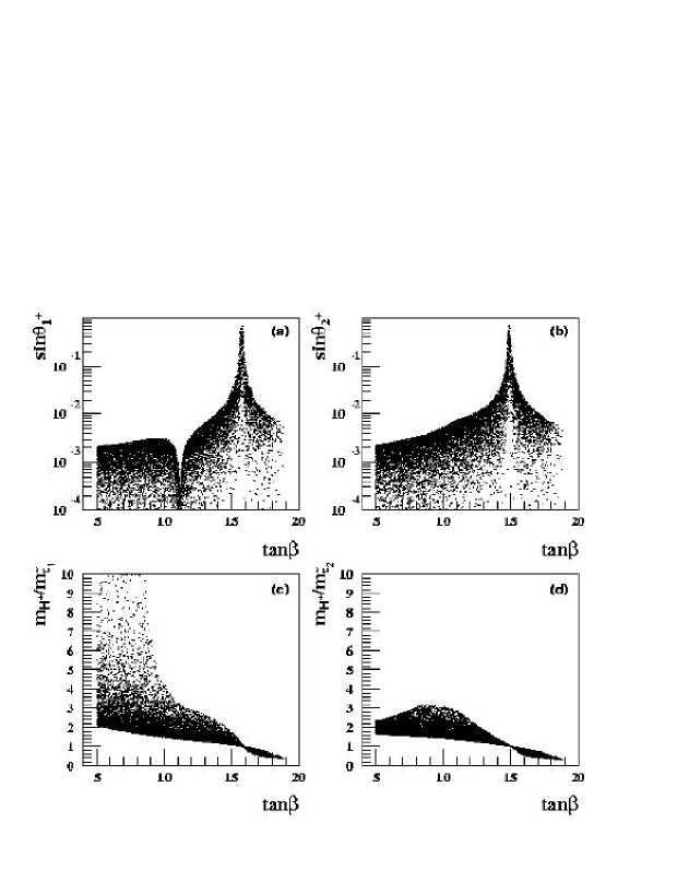
Figure 4: (a) Charged Higgs–light stau mixing; (b) Charged Higgs–heavy stau mixing; (c) charged Higgs–light stau mass ratio and (d) charged Higgs–heavy stau mass ratio as a function of $\tan\beta$ for $m_{3/2}=32$ TeV, $\mu<0$ and $100<m_{0}<300$ GeV.

Figure 4a (b) contains the mixing between the lightest (heaviest) stau and the charged Higgs fields $\sin\theta^{+}_{1(2)}$ as a function of $\tan\beta$ for $m_{3/2}=32$ TeV, $\mu<0$, and $100<m_{0}<300$ GeV. In this sector, the mixing can also be very large provided there is a near degeneracy between the staus $\tilde{\tau}^{\pm}_{1}$, $\tilde{\tau}^{\pm}_{2}$ and $H^{\pm}$. We can see clearly this effect in Fig. 4c (d), where we show the ratio between the charged Higgs mass $m_{H^{+}}$ and the lightest (heaviest) stau mass $m_{\tilde{\tau}_{1(2)}}$. In Figs. 4a and b we also notice that large light stau–charged Higgs mixing occurs at slight different value of $\tan\beta$ compared with heavy stau–charged Higgs mixing. Large light stau–charged Higgs mixing is found in Fig. 4a as a peak at $\tan\beta\approx 16$, as opposed to large heavy stau–charged Higgs mixing, which presents a peak at $\tan\beta\approx 15$. In Fig. 4a we notice that the mixing angle vanishes at $\tan\beta\sim 11$. This zero occurs at the point of parameter space where the two staus are nearly degenerated, as will be explained in Sec. 7.

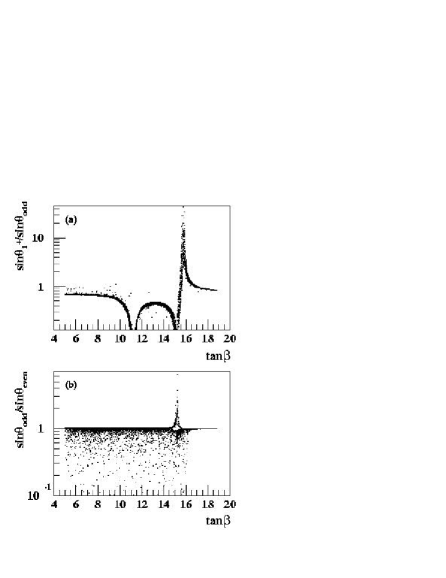
Figure 5: (a) Ratio between the charged Higgs–stau and CP–odd Higgs–tau–sneutrino mixing angles and (b) ratio between the CP–odd Higgs–tau–sneutrino and CP–even Higgs–tau–sneutrino mixing angles as a function of $\tan\beta$ for $m_{3/2}=32$ TeV, $\mu<0$ and $100<m_{0}<300$ GeV.

Similarly, in the last figure, the exact value of $\tan\beta$ at which the peak of the lightest stau–charged scalar mixing occurs is somewhat larger than the analogous mixing for the CP–odd sector $\sin\theta_{odd}$. This can be appreciated in Fig. 5a where we show the ratio between $\sin\theta_{1}^{+}$ and $\sin\theta_{odd}$ as a function of $\tan\beta$ for $m_{3/2}=32$ TeV, $\mu<0$ and $100<m_{0}<300$ GeV. The peak of the charged sector mixing is located at the peak of the ratio. On the other hand, the peak for the neutral CP–odd sector is located at the nearby zero of the ratio. The other zero of the ratio near $\tan\beta\approx 11$ corresponds to a zero of the charged scalar sector mixing, as shown in Fig. 4. For the sake of comparison, we display in Fig. 5b the ratio between the CP–odd and CP–even mixings ($\sin\theta_{odd}/\sin\theta_{even}$) as a function of $\tan\beta$. We can see that most of the time the ratio is equal to 1 showing that the two neutral scalar sectors have similar behavior with $\tan\beta$ in contrast with the charged scalar sector. The points where this ratio is lower than 1 correspond to the case where the CP–even scalar sector mixings are dominated by the light Higgs and tau–sneutrino degeneracy which occurs for any value of $\tan\beta$ lower than 16, as shown in Fig. 3c.

6 The Neutrino Mass

BRpV provides a solution to the atmospheric and solar neutrino problems due to their mixing with neutralinos, which generates neutrino masses and mixing angles. It was shown in [14] that the atmospheric mass scale is adequately described by the tree level neutrino mass

$$m_{\nu_{3}}^{tree}={{M_{1}g^{2}+M_{2}g^{\prime 2}}\over{4\Delta_{0}}}|\vec{\Lambda}|^{2}\;,$$ (35)

where $\Delta_{0}$ is the determinant of the neutralino sub–matrix and $\vec{\Lambda}=(\Lambda_{1},\Lambda_{2},\Lambda_{3})$, with

$$\Lambda_{i}=\mu v_{i}+\epsilon_{i}v_{d}\;,$$ (36)

where the index $i$ refers to the lepton family. The spectrum generated is hierarchical, and obtained typically with $\Lambda_{1}\ll\Lambda_{2}\approx\Lambda_{3}$.

As it was mentioned in the introduction, for many purposes it is enough to work with $R_{P}$ violation only in the third generation. In this case, the atmospheric mass scale is well described by Eq. (35) with the replacement $|\vec{\Lambda}|^{2}\rightarrow\Lambda_{3}^{2}$. In Fig. 6, we plot the neutrino mass as a function of $\Lambda$ in AMSB–BRpV with the input parameters $m_{3/2}=32$ TeV, $\mu<0$, $5<\tan\beta<20$, $100<m_{0}<1000$ GeV and $10^{-5}<\epsilon_{3}<1$ GeV. The quadratic dependence of the neutrino mass on $\Lambda$ is apparent in this figure and neutrino masses smaller than 1 eV occur for $|\Lambda|\mathrel{\vbox{\hbox{$<$}\nointerlineskip\hbox{$\sim$}}}0.6\,{\mathrm{GeV}}^{2}$. Moreover, the stars correspond to the allowed neutrino masses when the tau–sneutrino is the LSP. In general the points with a small (large) $m_{0}$ are located in the inner (outer) regions of this scattered plot.

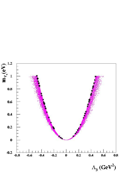
Figure 6: Tau neutrino mass as a function of $\Lambda_{3}$ for $5<\tan\beta<20$, $100<m_{0}<1000$ GeV, $m_{3/2}=32$ TeV and $\mu<0$.

From Fig. 6, we can see that the attainable neutrino masses are consistent with the global three–neutrino oscillation data analysis in the first reference of [10] that favors the $\nu_{\tau}\rightarrow\nu_{\mu}$ oscillation hypothesis. Although only mass squared differences are constrained by the neutrino data, our model naturally gives a hierarchical neutrino mass spectrum, therefore, we extract a naïve constraint on the actual mass coming from the analysis of the full atmospheric neutrino data, $0.04\mathrel{\vbox{\hbox{$<$}\nointerlineskip\hbox{$\sim$}}}m_{\nu_{\tau}}\mathrel{\vbox{\hbox{$<$}\nointerlineskip\hbox{$\sim$}}}0.09$ eV [10]. In addition, we notice that it is not possible to find an upper bound on the neutrino mass if angular dependence on the neutrino data is not included and only the total event rates are considered.

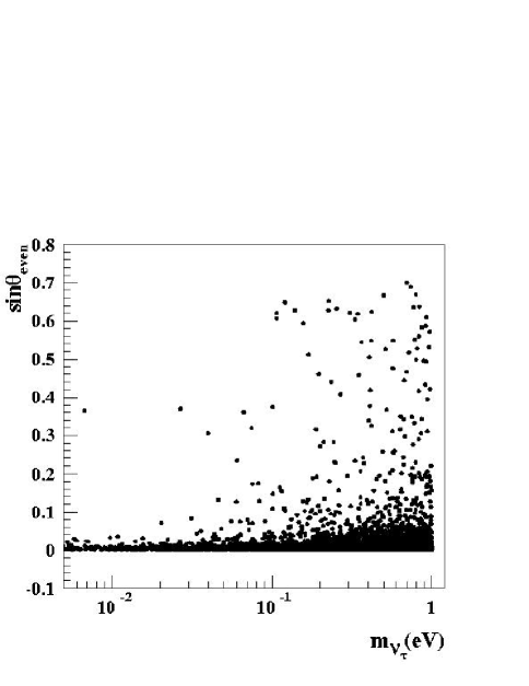
Figure 7: Mixing between CP–even Higgses and sneutrino as a function of the tau neutrino mass.

In Fig. 7 we show the correlation between the neutrino mass and mixing of the tau–sneutrino and the CP–even Higgses ($\sin\theta_{even}$) for the parameters assumed in Fig. 6. As expected, the largest mixings are associated to larger neutrino masses. Notwithstanding, it is possible to obtain large mixings for rather small neutrino masses because the mixing is proportional to the $R_{P}$ violating parameters $\epsilon_{3}$ and $v_{3}$, and not directly on $\Lambda_{3}\propto m_{\nu_{\tau}}$. In any case, Fig. 7 suggests that large scalar mixings are still possible even imposing these bounds on the neutrino mass. This is extremely important for the phenomenology of the model because it indicates that non negligible $R_{P}$ violating branching ratios are possible for scalars even in the case they are not the LSP.

7 Discussions

The presence of $R_{P}$ violating interactions in our model render the LSP unstable, avoiding strong constraints on the possible LSP candidates. In the parameter regions where the neutralino is not the LSP, whether the light stau or the tau–sneutrino is the LSP depends crucially on the value of $\tan\beta$. This fact can be seen in Fig. 8 where we plot the ratio between the light stau and the tau–sneutrino masses as a function of $\tan\beta$ for $m_{3/2}=32$ TeV, $100<m_{0}<300$ GeV, and $\mu<0$. From this figure we see that the tau–sneutrino is the LSP for $8.5\mathrel{\vbox{\hbox{$<$}\nointerlineskip\hbox{$\sim$}}}\tan\beta\mathrel{\vbox{\hbox{$<$}\nointerlineskip\hbox{$\sim$}}}14$, otherwise the stau is the LSP.

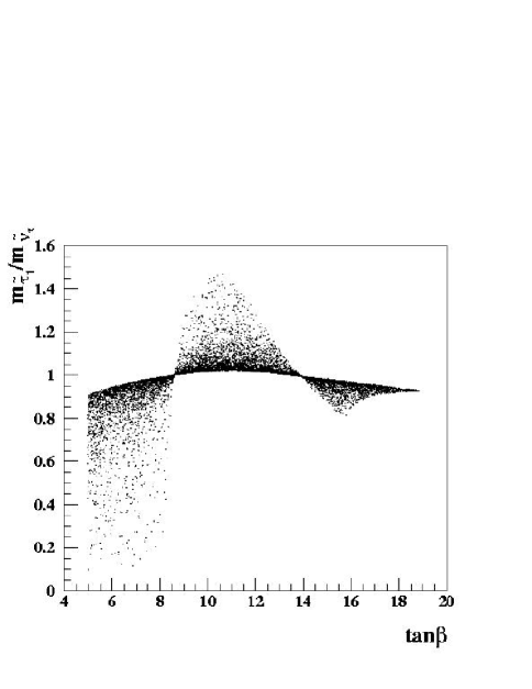
Figure 8: Ratio between the light stau and the sneutrino masses as a function of $\tan\beta$ for $m_{3/2}=32$ TeV, $100<m_{0}<300$ GeV and $\mu<0$.

When the stau is the LSP, it decays via $R_{P}$ violating interactions, i.e., its decays take place through mixing with the charged Higgs, and consequently, they will mimic the charged Higgs boson ones. Therefore, it is very important to be able to distinguish between $\tilde{\tau}^{\pm}_{1}$ and $H^{\pm}$. This can be achieved either through precise studies of branching ratios, or via the mass spectrum, or both [19].

Measurements on the mass spectrum are also important in order to distinguish AMSB with and without conservation of $R_{P}$. In Fig. 9 we present the ratio between the stau mass splitting in AMSB–BRpV and in the AMSB, $R=(m_{\tilde{\tau}_{2}}-m_{\tilde{\tau}_{1}})_{\rm AMSB-BRpV}/(m_{\tilde{\tau}_{2}}-m_{\tilde{\tau}_{1}})_{\rm AMSB}$, with $\epsilon_{3}=v_{3}=0$ and keeping the rest of the parameters unchanged, as a function of $\tan\beta$. In these figures, we took $100<m_{0}<1000$ GeV, $m_{3/2}=32$ TeV, and (a) $\mu>0$, and (b) $\mu<0$. For $\mu>0$ (Fig. 9a), the stau mass splitting is always larger in the AMSB–BRpV than in the AMSB by a factor that increases when $\tan\beta$ decreases, and can be as large as $R\sim 10$ for $\tan\beta\sim 3$! We remind the reader that, in the absence of $R_{P}$ violation, the left–right stau mixing decreases with decreasing $\tan\beta$, thus augmenting the importance of $R$–parity violating mixings. On the other hand, for $\mu<0$ (Fig. 9b), this ratio can be as large as before at small $\tan\beta$, but in addition, the splitting can go to zero in AMSB–BRpV near $\tan\beta\approx 11$, which also constitutes a sharp difference with the AMSB. For both signs of $\mu$ the ratio goes to unity at large $\tan\beta$ because the left–right mixing in the AMSB is proportional to $\tan\beta$ and dominates over any $R_{P}$ violating contribution.

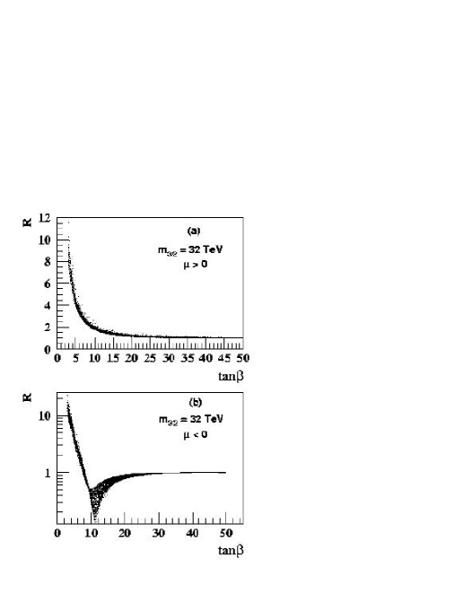
Figure 9: Ratio ($R$) between the stau splitting in AMSB with and without $R_{P}$ violation as a function of $\tan\beta$, for: $m_{3/2}=32$ TeV, $100<m_{0}<1000$ GeV and (a) $\mu>0$ or (b) $\mu<0$.

The behavior of $R$ at $\tan\beta\sim 11$ in Fig. 9b indicates that the two staus can be nearly degenerated in AMSB–BRpV. In Fig. 10 we plot the ratio between the light and heavy stau masses as a function of $\tan\beta$, for $m_{3/2}=32$ TeV, $100<m_{0}<300$ GeV and $\mu<0$, observing clearly that the near degeneracy occurs at $\tan\beta\sim 11$. In first approximation, consider that the near degeneracy occurs when $A_{\tau}v_{d}-\mu v_{u}\approx 0$ as inferred from Eq. (25). In addition, the mixing $X_{dR}$ in Eq. (31) is also very small because it is proportional to $\Lambda_{\tau}$ in Eq. (36), which defines the atmospheric neutrino mass, as indicated in Eq. (35). The smallness of these two quantities implies that the mixing $X_{uR}$ in Eq. (29) is also small in this particular region of parameter space, indicating that the right stau is decoupled from the Higgs fields and thus originating the zero in the mixing angle, noted already in Figs. 4 and 5.

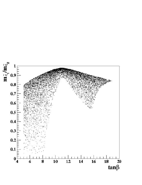
Figure 10: Ratio between the light and heavy stau masses as a function of $\tan\beta$ for $m_{3/2}=32$ TeV, $100<m_{0}<300$ GeV and $\mu<0$.

In order to quantify the stau mass splitting in our model, we present in Fig. 11 contours of constant splitting between the stau masses, $m_{\tilde{\tau}_{2}}-m_{\tilde{\tau}_{1}}$, in the plane $m_{3/2}\times m_{0}$ in GeV for $\mu<0$ and several $\tan\beta$. We can see in Fig. 11a that for small $\tan\beta=3$ the stau mass splitting in our model starts at $m_{\tilde{\tau}_{2}}-m_{\tilde{\tau}_{1}}\sim 30$ GeV, in sharp contrast with the $R_{P}$ conserving case where the biggest splittings barely goes over this value [7]. This is in agreement with the results presented in Fig. 9b. Furthermore, we can also see that there is a considerable region in the $m_{3/2}\times m_{0}$ plane, indicated by the grey area, where the lightest stau is the LSP. For intermediary values of $\tan\beta\sim 15$, Fig. 11b shows that the stau mass splitting goes to a minimum. This is a different behavior from the MSSM which presents a mass splitting up to 10 times bigger as we have seen in Fig. 9b. For this value of $\tan\beta$ we still have a small region where the lightest stau is the LSP (grey area) and, as a novelty, a tiny region for small values of $m_{3/2}$ and $m_{0}$ where the tau–sneutrino is the LSP (black area). For large values of $\tan\beta=30$, the stau splitting mass shown in Fig. 11c is similar to the MSSM one [7].

Figure 11: Contours of constant splitting between the light stau and heavy stau masses in the plane $m_{3/2}\times m_{0}$ in GeV for $\mu<0$, $\tan\beta=3$ (a), 15 (b) and 30 (c). The hatched area is theoretically forbidden; the grey area in (a) and (b) is where the lightest stau is the LSP, while the small black area in (b) is where the tau–sneutrino is the LSP.

We have made below a series of three figures fixing the value $\tan\beta=15$ to study the dependence on $m_{0}$ of the mass spectrum and mixings in the scalar sector. This choice of $\tan\beta$ is such that we find a degeneracy among the masses, and consequently we obtain large mixings in the scalar sector. We also chose $m_{3/2}=32$ TeV and $\mu<0$, while the $R_{P}$ violating parameters were varied according to $10^{-5}<\epsilon_{3}<1$ GeV and $10^{-6}<m_{\nu_{\tau}}<1$ eV.

In Fig. 12a we plot tau–sneutrino mixing with the CP–odd neutral Higgs as a function of $m_{0}$ for the parameters indicated above. We find quite large mixings for $m_{0}\approx 320$ GeV. In Fig. 12b we show the CP–odd Higgs and tau–sneutrino masses, which depend almost linearly on $m_{0}$. Moreover, the value of $m_{0}$ at which these two particles have the same mass coincides with the point of maximum mixing.

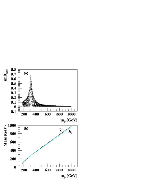
Figure 12: (a) Mixing of the CP–odd Higgs and the sneutrino and (b) the CP–odd Higgs and sneutrino masses as a function of $m_{0}$ for $m_{3/2}=32$ TeV, $\mu<0$ and $\tan\beta=15$.

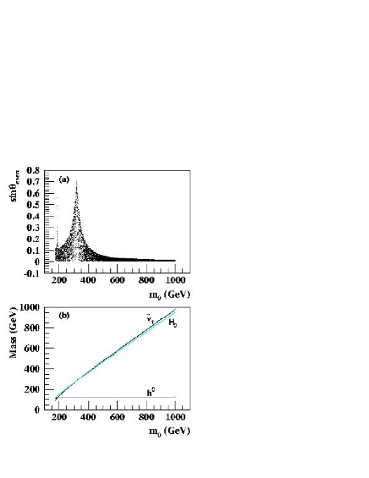
Figure 13: (a) Mixing between the CP–even Higgs and sneutrino and (b) the light and heavy CP–even Higgs masses as well as the sneutrino one as a function of $m_{0}$ for $m_{3/2}=32$ TeV, $\mu<0$ and $\tan\beta=15$.

The CP–even tau–sneutrino mixing with the CP–even Higgs is presented in Fig. 13a as a function of $m_{0}$. There are two peaks of high mixing; the main one at $m_{0}\approx 320$ GeV and a narrow one at $m_{0}\approx 180$ GeV. These two peaks have a different origin, as indicated by Fig. 13b, where we plot the masses of the two CP–even neutral Higgs bosons, $m_{h}$ and $m_{H}$, and the mass of the CP–even tau–sneutrino $m_{\tilde{\nu}_{\tau}^{even}}$, as a function of $m_{0}$. We observe that the broad peak is due to a degeneracy between the tau–sneutrino and the heavy neutral Higgs boson and the narrow peak comes from a degeneracy between the tau–sneutrino and the light neutral Higgs boson. As expected, the $H^{0}$ and $\tilde{\nu}_{\tau}^{even}$ masses grow linearly with $m_{0}$, contrary to the $h^{0}$ mass which remains almost constant.

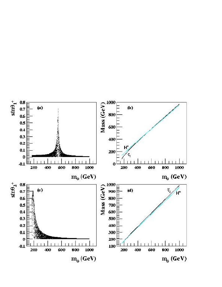
Figure 14: (a) Mixing of the charged Higgs with the light stau, (b) charged Higgs and light stau masses, (c) mixing of the charged Higgs with the heavy stau, and (d) charged Higgs and heavy stau masses as a function of $m_{0}$ for $m_{3/2}=32$ TeV, $\mu<0$ and $\tan\beta=15$.

In Figure 14a we display the light stau mixing with the charged Higgs as a function of $m_{0}$. The maximum mixing, obtained at $m_{0}\approx 550$ GeV, is the result of a mass degeneracy between the charged Higgs boson and the light stau. This can be observed in Fig. 14b where we plot the charged Higgs mass $m_{H^{\pm}}$ and the light stau mass $m_{\tilde{\tau}_{1}}$ as a function of $m_{0}$.

In a similar way, we show the heavy stau mixing with charged Higgs as a function of $m_{0}$ in Fig. 14c, where we observe a maximum for the mixing at $m_{0}\approx 200$ GeV. This large mixing is due to a degeneracy between the charged Higgs boson and the heavy stau masses, as can be seen in Fig. 14d. One can notice that all charged scalars show an almost linear dependency of their mass on the mass parameter $m_{0}$.

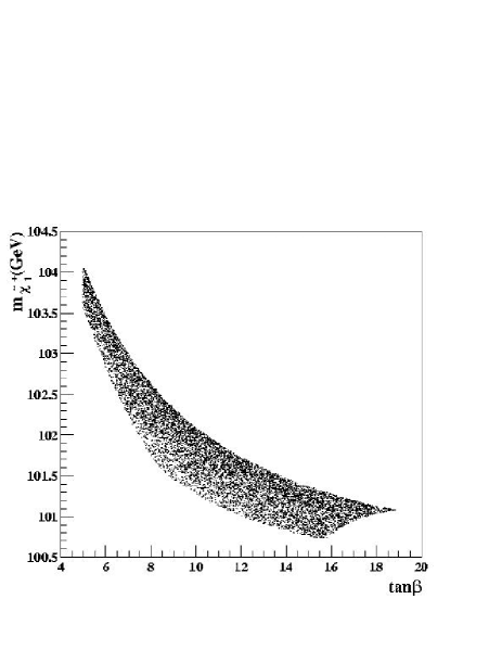
Figure 15: Light chargino mass as a function of $\tan\beta$ for $m_{3/2}=32$ TeV, $\mu<0$ and $100<m_{0}<300$ GeV.

As opposed to the scalar sector, where mixing between the Higgs bosons and sleptons can be maximum, in the chargino and neutralino sectors the mixings with leptons are controlled by the neutrino mass being very small. Despite this fact, the mixing in the neutralino sector is sufficient to generate adequate masses for the neutrinos and give rise to the neutralino decays mentioned in the introduction. Therefore, in the chargino sector the BRpV–AMSB phenomenology changes very little with respect to the $R_{P}$ conserving AMSB. One of the distinctive features of AMSB that differentiates it from other scenarios of supersymmetry breaking in the chargino–neutralino sector is the near degeneracy between the lightest chargino and the lightest neutralino. This feature remains in BRpV–AMSB as was anticipated in Fig. 1. For $m_{3/2}=32$ TeV, $\mu<0$, and $100<m_{0}<300$ GeV, we show in Fig. 15 the lightest chargino mass as a function of $\tan\beta$. The lightest chargino mass has a small dependence on $\tan\beta$ since its value varies only between 100 and 104 GeV. As in $R_{P}$ conserving AMSB, the mass difference $m_{\tilde{\chi}^{+}_{1}}-m_{\tilde{\chi}^{0}_{1}}$ remains small.

8 Conclusions

We have shown in the previous sections that our model exhibiting Anomaly Mediated Supersymmetry Breaking and Bilinear $R_{P}$ Violation is phenomenologically viable. In particular, the inclusion of BRpV generates neutrino masses and mixings in a natural way. Moreover, the $R_{P}$ breaking terms give rise to mixing between the Higgs bosons and the sleptons, which can be rather large despite the smallness of the parameters needed to generate realistic neutrino masses. These large mixings occur in regions of the parameter space where two states are nearly degenerate. Our model also alters substantially the mass splitting between the scalar taus in a large range of $\tan\beta$.

The $R_{P}$ violating interactions render the LSP unstable since it can decay via its mixing with the SM particles (leptons or scalars). Therefore, the constraints on the LSP are relaxed and forbidden regions of parameter space become allowed, where scalar particles like staus or sneutrinos are the LSP. Furthermore, the large mixing between Higgs bosons and sleptons has the potential to change the decays of these particles. These facts have a profound impact in the phenomenology of the model, changing drastically the signals at colliders [20].

Acknowledgements: This work was partially supported by a joint grant from Fundación Andes and Fundación Vitae, by DIPUC, by CONICYT grant No. 1010974, by Fundação de Amparo à Pesquisa do Estado de São Paulo (FAPESP), by Conselho Nacional de Desenvolvimento Científico e Tecnológico (CNPq) and by Programa de Apoio a Núcleos de Excelência (PRONEX).

Appendix A AMSB Boundary Conditions

The AMSB boundary conditions at the GUT scale for the gaugino masses are proportional to their beta functions, resulting in

$$M_{1} = {{33}\over 5}{{g_{1}^{2}}\over{16\pi^{2}}}m_{3/2}\;,$$ (37)

$$M_{2} = {{g_{2}^{2}}\over{16\pi^{2}}}m_{3/2}\;,$$ (38)

$$M_{3} = -3{{g_{3}^{2}}\over{16\pi^{2}}}m_{3/2}\;,$$ (39)

while the third generation scalar masses are given by

$$m_{U}^{2} = \left(-{88\over 25}g_{1}^{4}+8g_{3}^{4}+2f_{t}\hat{\beta}_{f_{t}}\right){m_{3/2}^{2}\over(16\pi^{2})^{2}}+m_{0}^{2}\;,$$ (40)

$$m_{D}^{2} = \left(-{22\over 25}g_{1}^{4}+8g_{3}^{4}+2f_{b}\hat{\beta}_{f_{b}}\right){m_{3/2}^{2}\over(16\pi^{2})^{2}}+m_{0}^{2}\;,$$ (41)

$$m_{Q}^{2} = \left(-{11\over 50}g_{1}^{4}-{3\over 2}g_{2}^{4}+8g_{3}^{4}+f_{t}\hat{\beta}_{f_{t}}+f_{b}\hat{\beta}_{f_{b}}\right){m_{3/2}^{2}\over(16\pi^{2})^{2}}+m_{0}^{2}\;,$$ (42)

$$m_{L}^{2} = \left(-{99\over 50}g_{1}^{4}-{3\over 2}g_{2}^{4}+f_{\tau}\hat{\beta}_{f_{\tau}}\right){m_{3/2}^{2}\over(16\pi^{2})^{2}}+m_{0}^{2}\;,$$ (43)

$$m_{E}^{2} = \left(-{198\over 25}g_{1}^{4}+2f_{\tau}\hat{\beta}_{f_{\tau}}\right){m_{3/2}^{2}\over(16\pi^{2})^{2}}+m_{0}^{2}\;,$$ (44)

$$m_{H_{u}}^{2} = \left(-{99\over 50}g_{1}^{4}-{3\over 2}g_{2}^{4}+3f_{t}\hat{\beta}_{f_{t}}\right){m_{3/2}^{2}\over(16\pi^{2})^{2}}+m_{0}^{2}\;,$$ (45)

$$m_{H_{d}}^{2} = \left(-{99\over 50}g_{1}^{4}-{3\over 2}g_{2}^{4}+3f_{b}\hat{\beta}_{f_{b}}+f_{\tau}\hat{\beta}_{f_{\tau}}\right){m_{3/2}^{2}\over(16\pi^{2})^{2}}+m_{0}^{2}\;.$$ (46)

Finally, the $A$–parameters are given by

$$A_{t} = {\hat{\beta}_{f_{t}}\over f_{t}}{m_{3/2}\over 16\pi^{2}}\;,$$ (47)

$$A_{b} = {\hat{\beta}_{f_{b}}\over f_{b}}{m_{3/2}\over 16\pi^{2}}\;,$$ (48)

$$A_{\tau} = {\hat{\beta}_{f_{\tau}}\over f_{\tau}}{m_{3/2}\over 16\pi^{2}}\;,$$ (49)

where we have defined

$$\hat{\beta}_{f_{t}} = 16\pi^{2}\beta_{t}=f_{t}\left(-{13\over 15}g_{1}^{2}-3g_{2}^{2}-{16\over 3}g_{3}^{2}+6f_{t}^{2}+f_{b}^{2}\right)\;,$$ (50)

$$\hat{\beta}_{f_{b}} = 16\pi^{2}\beta_{b}=f_{b}\left(-{7\over 15}g_{1}^{2}-3g_{2}^{2}-{16\over 3}g_{3}^{2}+f_{t}^{2}+6f_{b}^{2}+f_{\tau}^{2}\right)\;,$$ (51)

$$\hat{\beta}_{f_{\tau}} = 16\pi^{2}\beta_{\tau}=f_{\tau}\left(-{9\over 5}g_{1}^{2}-3g_{2}^{2}+3f_{b}^{2}+4f_{\tau}^{2}\right)\;.$$ (52)

Appendix B The Renormalization Group Equations

Here we present the one–loop renormalization group equations for our model, assuming the bilinear $R_{P}$ breaking terms are restricted only to the third generation. First, we display the equations for the Yukawa couplings of the trilinear terms

$$16\pi^{2}\frac{dh_{U}}{dt}=h_{U}\left(6h_{U}^{2}+h_{D}^{2}-\frac{16}{3}g_{3}^{2}-3g_{2}^{2}-\frac{13}{9}g_{1}^{2}\right)\;,$$ (53)

$$16\pi^{2}\frac{dh_{D}}{dt}=h_{D}\left(6h_{D}^{2}+h_{U}^{2}+h_{\tau}^{2}-\frac{16}{3}g_{3}^{2}-3g_{2}^{2}-\frac{7}{9}g_{1}^{2}\right)\;,$$ (54)

$$16\pi^{2}\frac{dh_{\tau}}{dt}=h_{\tau}\left(4h_{\tau}^{2}+3h_{D}^{2}-3g_{2}^{2}-3g_{1}^{2}\right)\;.$$ (55)

The corresponding RGE for cubic soft supersymmetry breaking parameters are given by

$$8\pi^{2}\frac{dA_{U}}{dt}=6h_{U}^{2}A_{U}+h_{D}^{2}A_{D}+\frac{16}{3}g_{3}^{2}M_{3}+3g_{2}^{2}M_{2}+\frac{13}{9}g_{1}^{2}M_{1}\;,$$ (56)

$$8\pi^{2}\frac{dA_{D}}{dt}=6h_{D}^{2}A_{D}+h_{U}^{2}A_{U}+h_{\tau}^{2}A_{\tau}+\frac{16}{3}g_{3}^{2}M_{3}+3g_{2}^{2}M_{2}+\frac{7}{9}g_{1}^{2}M_{1}\;,$$ (57)

$$8\pi^{2}\frac{dA_{\tau}}{dt}=4h_{\tau}^{2}A_{\tau}+3h_{D}^{2}A_{D}+3g_{2}^{2}M_{2}+3g_{1}^{2}M_{1}\;.$$ (58)

For the soft supersymmetry breaking mass parameters we have

$$8\pi^{2}\frac{dM_{Q}^{2}}{dt} = h_{U}^{2}(m_{H_{2}}^{2}+M_{Q}^{2}+M_{U}^{2}+A_{U}^{2})+h_{D}^{2}(m_{H_{1}}^{2}+M_{Q}^{2}+M_{D}^{2}+A_{D}^{2})$$ (60)

$$-\frac{16}{3}g_{3}^{2}M_{3}^{2}-3g_{2}^{2}M_{2}^{2}-\frac{1}{9}g_{1}^{2}M_{1}^{2}+\frac{1}{6}~{}g_{1}^{2}{\cal S}\;,$$

$$8\pi^{2}\frac{dM_{U}^{2}}{dt}=2h_{U}^{2}(m_{H_{2}}^{2}+M_{Q}^{2}+M_{U}^{2}+A_{U}^{2})-\frac{16}{3}g_{3}^{2}M_{3}^{2}-\frac{16}{9}g_{1}^{2}M_{1}^{2}-\frac{2}{3}~{}g_{1}^{2}{\cal S}\;,$$ (61)

$$8\pi^{2}\frac{dM_{D}^{2}}{dt}=2h_{D}^{2}(m_{H_{1}}^{2}+M_{Q}^{2}+M_{D}^{2}+A_{D}^{2})-\frac{16}{3}g_{3}^{2}M_{3}^{2}-\frac{4}{9}g_{1}^{2}M_{1}^{2}+\frac{1}{3}~{}g_{1}^{2}{\cal S}\;,$$ (62)

$$8\pi^{2}\frac{dM_{L}^{2}}{dt}=h_{\tau}^{2}(m_{H_{1}}^{2}+M_{L}^{2}+M_{R}^{2}+A_{\tau}^{2})-3g_{2}^{2}M_{2}^{2}-g_{1}^{2}M_{1}^{2}-\frac{1}{2}~{}g_{1}^{2}{\cal S}\;,$$ (63)

$$8\pi^{2}\frac{dM_{R}^{2}}{dt}=2h_{\tau}^{2}(m_{H_{1}}^{2}+M_{L}^{2}+M_{R}^{2}+A_{\tau}^{2})-4g_{1}^{2}M_{1}^{2}+g_{1}^{2}{\cal S}\;,$$ (64)

$$8\pi^{2}\frac{dm_{H_{2}}^{2}}{dt}=3h_{U}^{2}(m_{H_{2}}^{2}+M_{Q}^{2}+M_{U}^{2}+A_{U}^{2})-3g_{2}^{2}M_{2}^{2}-g_{1}^{2}M_{1}^{2}+\frac{1}{2}~{}g_{1}^{2}{\cal S}\;,$$ (65)

$$8\pi^{2}\frac{dm_{H_{1}}^{2}}{dt} = 3h_{D}^{2}(m_{H_{1}}^{2}+M_{Q}^{2}+M_{D}^{2}+A_{D}^{2})+h_{\tau}^{2}(m_{H_{1}}^{2}+M_{L}^{2}+M_{R}^{2}+A_{\tau}^{2})$$ (67)

$$-3g_{2}^{2}M_{2}^{2}-g_{1}^{2}M_{1}^{2}-\frac{1}{2}~{}g_{1}^{2}{\cal S}\;,$$

where

$${\cal S}=m_{H_{2}}^{2}-m_{H_{1}}^{2}+M_{Q}^{2}-2M_{U}^{2}+M_{D}^{2}-M_{L}^{2}+M_{R}^{2}\;.$$ (68)

For the bilinear terms in the superpotential we get

$$16\pi^{2}\frac{d\mu}{dt}=\mu\left(3h_{U}^{2}+3h_{D}^{2}+h_{\tau}^{2}-3g_{2}^{2}-g_{1}^{2}\right)\;,$$ (69)

$$16\pi^{2}\frac{d\epsilon_{3}}{dt}=\epsilon_{3}\left(3h_{U}^{2}+h_{\tau}^{2}-3g_{2}^{2}-g_{1}^{2}\right)\;,$$ (70)

and for the corresponding soft breaking terms

$$8\pi^{2}\frac{dB}{dt}=3h_{U}^{2}A_{U}+3h_{D}^{2}A_{D}+h_{\tau}^{2}A_{\tau}+3g_{2}^{2}M_{2}+g_{1}^{2}M_{1}\;,$$ (71)

$$8\pi^{2}\frac{dB_{2}}{dt}=3h_{U}^{2}A_{U}+h_{\tau}^{2}A_{\tau}+3g_{2}^{2}M_{2}+g_{1}^{2}M_{1}\;.$$ (72)

The $g_{i}$ are the $SU(3)\times SU(2)\times U(1)$ gauge couplings and the $M_{i}$ are the corresponding soft breaking gaugino masses.

References

- [1] A. Chamseddine, R. Arnowitt and P. Nath, Phys. Rev. Lett. 49, 970 (1982); R. Barbieri, S. Ferrara and C. Savoy, Phys. Lett. B 119, 343 (1982); L. J. Hall, J. Lykken and S. Weinberg, Phys. Rev. D 27, 2359 (1983).
- [2] M. Dine and A. Nelson, Phys. Rev. D 48, 1277 (1993); M. Dine, A. Nelson and Y. Shirman, Phys. Rev. D 51, 1362 (1995); M. Dine, A. Nelson, Y. Nir and Y. Shirman, Phys. Rev. D 53, 2658 (1996).
- [3] L. Randall and R. Sundrum, Nucl. Phys. B 557, 79 (1999); G. Giudice, M. Luty, H. Murayama and R. Rattazzi, JHEP 9812, 027 (1998).
- [4] T. Gherghetta, G. F. Giudice and J. D. Wells, Nucl. Phys. B 559, 27 (1999).
- [5] A. Pomarol and R. Rattazzi, JHEP 9905, 013 (1999); Z. Chacko, M. A. Luty, I. Maksymyk and E. Ponton, JHEP 0004, 001 (2000); E. Katz, Y. Shadmi and Y. Shirman, JHEP 9908, 015 (1999); M. A. Luty and R. Sundrum, Phys. Rev. D 62, 035008 (2000); J. A. Bagger, T. Moroi and E. Poppitz, JHEP 0004, 009 (2000); I. Jack and D. R. T. Jones, Phys. Lett. B 482, 167 (2000); M. Kawasaki, T. Watari and T. Yanagida, Phys. Rev. D 63, 083510 (2001).
- [6] T. Moroi and L. Randall, Nucl. Phys. B 570, 455 (2000); G. D. Kribs, Phys. Rev. D 62, 015008 (2000); S. Su, Nucl. Phys. B 573, 87 (2000); R. Rattazzi, A. Strumia and J. D. Wells, Nucl. Phys. B 576, 3 (2000); M. Carena, K. Huitu and T. Kobayashi, Nucl. Phys. B 592, 164 (2001); H. Baer, M. A. Díaz, P. Quintana and X. Tata, JHEP 0004, 016 (2000); D. K. Ghosh, P. Roy and S. Roy, JHEP 0008, 031 (2000); U. Chattopadhyay, D. K. Ghosh and S. Roy, Phys. Rev. D 62, 115001 (2000); H. Baer, J. K. Mizukoshi and X. Tata, Phys. Lett. B 488, 367 (2000).
- [7] J. L. Feng and T. Moroi, Phys. Rev. D 61, 095004 (2000).
- [8] B. C. Allanach and A. Dedes, JHEP 0006, 017 (2000).
- [9] B. Allanach et al., hep–ph/9906224; B. Allanach et al., J. Phys. G 24, 421 (1998).
- [10] M. C. Gonzalez–García, M. Maltoni, C. Peña–Garay and J. W. F. Valle, Phys. Rev. D 63, 033005 (2001); J. N. Bahcall, P. I. Krastev and A. Yu. Smirnov, JHEP 0105, 015 (2001).
- [11] Y. Fukuda et al., Super–Kamiokande Collaboration, Phys. Rev. Lett. 81, 1562 (1998); Phys. Lett. B 433, 9 (1998); Phys. Lett. B 436, 33 (1998).
- [12] F. de Campos, O. J. P. Éboli, M. A. García–Jareño and J. W. F. Valle, Nucl. Phys. B 546, 33 (1999); R. Kitano and K. Oda, Phys. Rev. D 61, 113001 (2000); D. E. Kaplan and A. E. Nelson, JHEP 0001, 033 (2000); C.–H. Chang and T.–F. Feng, Eur. Phys. J. C12, 137 (2000); M. Frank, Phys. Rev. D 62, 015006 (2000); F. Takayama and M. Yamaguchi, Phys. Lett. B 476, 116 (2000); K. Choi, E. J. Chun and K. Hwang, Phys. Lett. B 488, 145 (2000); J. M. Mira, E. Nardi, D. A. Restrepo and J. W. F. Valle, Phys. Lett. B 492, 81 (2000).
- [13] R. Hempfling, Nucl. Phys. B 478, 3 (1996).
- [14] J. C. Romão, M. A. Díaz, M. Hirsch, W. Porod and J. W. F. Valle, Phys. Rev. D 61, 071703 (2000); M. Hirsch, M. A. Díaz, W. Porod, J. C. Romão and J. W. F. Valle, Phys. Rev. D 62, 113008 (2000).
- [15] T. Banks, Y. Grossman, E. Nardi and Y. Nir, Phys. Rev. D 52, 5319 (1995); M. Nowakowski and A. Pilaftsis, Nucl. Phys. B 461, 19 (1996); G. Bhattacharyya, D. Choudhury and K. Sridhar, Phys. Lett. B 349, 118 (1995); H. Nilles and N. Polonsky, Nucl. Phys. B 484, 33 (1997); A. Yu. Smirnov and F. Vissani, Nucl. Phys. B 460, 37 (1996); J. C. Romão, F. de Campos, M. A. García–Jareño, M. B. Magro and J. W. F. Valle, Nucl. Phys. B 482, 3 (1996); B. de Carlos and P. L. White, Phys. Rev. D 54, 3427 (1996); B. de Carlos and P. L. White, Phys. Rev. D 55, 4222 (1997).
- [16] A. Santamaria and J. W. F. Valle, Phys. Lett. B 195, 423 (1987); Phys. Rev. Lett. 60, 397 (1988); Phys. Rev. D 39, 1780 (1989).
- [17] M. A. Díaz, J. C. Romão and J. W. F. Valle, Nucl. Phys. B 524, 23 (1998).
- [18] A. Akeroyd, M. A. Díaz, J. Ferrandis, M. A. García–Jareño and J. W. F. Valle, Nucl. Phys. B 529, 3 (1998); M. A. Díaz, J. Ferrandis, J. C. Romão and J. W. F. Valle, Phys. Lett. B 453, 263 (1999); A. G. Akeroyd, M. A. Díaz and J. W. F. Valle, Phys. Lett. B 441, 224 (1998); M. A. Díaz, E. Torrente–Lujan and J. W. F. Valle, Nucl. Phys. B 551, 78 (1999); M. A. Díaz, J. Ferrandis, J. C. Romão and J. W. F. Valle, Nucl. Phys. B 590, 3 (2000); M. A. Díaz, D. A. Restrepo and J. W. F. Valle, Nucl. Phys. B 583, 182 (2000); M. A. Díaz, J. Ferrandis and J. W. F. Valle, Nucl. Phys. B 573, 75 (2000).
- [19] A. G. Akeroyd, C. Liu and J. Song, hep–ph/0107218.
- [20] F. de Campos et al., in preparation.