Resurrecting the KH78/80 partial wave analysis

P. Piirola^a, E. Pietarinen^a,b, and M.E. Sainio^a,b

^aDepartment of Physics,
^bHelsinki Institute of Physics,
P.O. Box 64, 00014 University of Helsinki, Finland

(Received: )
Most of the data from the meson factories were available only after the $\pi N$ partial wave analysis of Koch and Pietarinen [1] was published over 20 years ago. Since then, both the experimental precision and the theoretical framework have evolved a lot as well as the computing technology. Both the new and the earlier data are to be analysed by a highly modernised version of the earlier approach. Especially the propagation of the measurement errors in the analysis will be considered in detail, visualisation tools will be developed using the Python/Tkinter combination [2], and the huge data base of experiments will be handled by MySQL [3].

1 Introduction

About 20 years ago Koch and Pietarinen performed an energy-independent partial-wave analysis on pion-nucleon elastic and charge-exchange differential cross sections and elastic polarisations for laboratory momenta below 500 MeV/c incorporating the constraints from fixed-$t$ dispersion relations as well as crossing and unitarity (the KH78 and KH80 analyses) [1]. Since then, however, new low-energy data have emerged in all charge channels: examples of recent high precision results for the differential cross sections are given in refs. [4, 5, 6], polarisation parameter in refs. [7, 8, 9] and the spin rotation parameter in ref. [10]. There are also some new measurements of integrated cross sections [11]. Especially the high precision measurements of the hadronic level shift and width on pionic hydrogen and deuterium [12], giving information of the pion-nucleon interaction just at the threshold, have opened a completely new chapter in the study of the low-energy pion-nucleon interaction. Another direction where significant advances have taken place is the theoretical framework where we study the low-energy pion-nucleon interaction. The tool, chiral perturbation theory ($\chi$PT), has been developed in the 80’s and 90’s and the work continues. The development of $\chi$PT motivates a new partial wave analysis from the theoretical point of view — on one hand strong interaction physics is becoming a precision science also in the low-energy region, on the other hand, there is need for $\pi N$ phenomenology to fix some of the low-energy constants appearing in the meson-baryon lagrangian. See, for example, the talk of Meißner in these proceedings [13].

It is our goal to make use of the new data in an analysis which, in addition to the requirements of analyticity, crossing and unitarity, includes the constraints from chiral symmetry.

2 The old KH78/80 analysis

The aim of the KH analysis was to determine the amplitudes satisfying several conditions:

1. The amplitudes had to reproduce all the data which were available at that time, which means $\frac{d\sigma}{d\Omega}$, $\sigma_{\mathrm{tot}}$ and $P$ within their associated errors.

2. The solution had to fulfil the isospin invariance.

3. All partial waves had to satisfy the unitarity condition.

4. The crossing symmetry was implicitly assumed, because Mandelstam variables were used.

5. The invariant amplitudes were going to have the correct analyticity properties in $s$ at fixed-$t$.

6. The amplitudes at fixed-$s$ were to be analytic in $\cos\theta$ in the small Lehman ellipse.

The experimental data is not enough to fix a unique partial wave solution, but further theoretical constraints are needed. The constraints from fixed-$t$ analyticity and from the isospin invariance are strong enough to resolve the ambiguities [14].

3 Three stages of the analysis

3.1 Fixed-$t$ analysis

The old KH analyses consist of three phases: fixed-$t$ analysis, fixed-$\theta$ analysis and fixed-$s$ analysis, which were iterated until the results agreed up to about 3 %. The fixed-$t$ analysis was carried out at 40 $t$-values in the range from zero to $-1.0$ GeV². The analysis would be too complicated, if one were working with dispersion integrals, so the expansion [15, 16]

$$C(\nu,t)=C_{N}(\nu,t)+H(Z,t)\sum_{i=0}^{n}c_{i}Z^{i}$$ (1)

was used for $t$-values smaller than $-4m\mu$, ($\nu=(s-u)/4m_{N}$). In the expansion the nucleon pole term $C_{N}(\nu,t)$ is treated separately, and the sum is multiplied by a factor $H(Z,t)$, which describes the expected asymptotic behaviour. The essence of the expansion is that the sum is written in terms of functions $Z$, which have the correct analytic behaviour, i.e. it is not a polynomial approximation, but a series presentation of an analytic function, which is just truncated at some reasonable point (ca. $n=50$ or $n=100$), because infinite accuracy is impossible. The condition of smoothness and the compatibility with the data constrain the terms with large index $i$ to be negligible [15, 16].

The expansion coefficients $c_{i}$ are determined by minimising

$$\chi^{2}=\chi^{2}_{\mathrm{data}}+\chi^{2}_{\mathrm{pw}}+\chi^{2}_{\mathrm{penalty}}\;.$$ (2)

Here $\chi^{2}_{\mathrm{data}}$ comes from the experimental errors, $\chi^{2}_{\mathrm{pw}}$ belongs to the deviation from the fixed-$s$ partial wave solution and the last term is used to suppress large values of the higher coefficients of the expansion. In practice, the analyticity constraints cannot be used without smoothing the data. The aim is, of course, to smooth out the statistical fluctuations without distorting the physically relevant structures.

3.2 Fixed-$\theta$ analysis

The fixed-$t$ constraint is often used only for $t$ values from zero to about $-0.5$ GeV², because the partial wave expansions for the imaginary parts of the invariant amplitudes do not converge for large $|t|$. In the range $t\in(-0.5,-1.5]$ GeV² the truncated partial wave expansions can still be reasonable approximations, but for $t$ values below ca. $-1$ or $-1.5$ GeV² the fixed-$t$ analyticity cannot be applied anymore. So another analyticity constraint is used to cover the rest of the angular range at intermediate and at high energies. The calculation was made at 18 angles between $\cos\theta=-0.9\ldots 0.8$. Analysing methods are the same as in the fixed-$t$ analysis: the expansion method is used and the coefficients are fixed by minimising $\chi^{2}$, i.e. by fitting to the data and to the fixed-$t$ solution.

3.3 Fixed-$s$ analysis

The third stage, the fixed-$s$ analysis, is a standard phase shift analysis in the sense that the partial waves are fitted to the data. On the other hand, it is not the usual one, because the partial waves are fitted also to the fixed-$t$ and to the fixed-$\theta$ amplitudes. Now 92 momentum values were selected from the energy range $0\ldots 200$ GeV/c, 6 of the momenta were above 6 GeV/c. Again, the coefficients were fixed by minimising $\chi^{2}$ which now included also a term suitable to enforce unitarity.

4 Treatment of the data

The electromagnetic corrections proposed by Tromborg et al. at momentum values below $0.65$ GeV/c [17], were applied to the data. At higher momentum, only the one-photon exchange correction was applied, taking into account the Coulomb phase. In all three different analyses, the data were shifted to the selected energy bins (i.e. the selected values of $s$, $t$ or $\theta$) using the previous solution of the iteration to calculate the correction. Some data points requiring too large a momentum shift were omitted. The normalisation of some data sets had to be corrected to guarantee a smooth extrapolation to the forward direction, and to the input for the forward amplitude.

5 Life after KH80

The latest KH phase shift analysis was finished in 1980. After that there has been very accurate measurements of pionic hydrogen level shift and width, $\frac{d\sigma}{d\Omega}$ has been measured with good accuracy, many spin rotation parameter measurements has been done as well as polarisation parameter measurements. Also, some integrated cross section measurements have been performed. The newer data has never been analysed by the methods of Koch and Pietarinen, and for example the results of Pavan et al. [4] are not compatible with the results of the old analyses. So, an updated version of the analysis is certainly needed.

6 The code of Pietarinen

The original code was made for the NDP Fortran compiler, which runs under MS-DOS. The code needs to be ported to UNIX. We have tested the code in an old MS-DOS machine, and most of the main tasks seem to be working correctly. What is still needed, is a modification of the $s$-plane conformal mapping. This has effects on all routines, which are related to the fixed-$t$ analysis. Also some modifications are needed to be able to study the isospin analysis.

The code base is divided into several parts:

• There is a program for comparing the partial wave solution to existing data. It simply plots the data and the solution in the same picture, and allows the comparison of different data sets to the solution.

• The second part is for shifting the experimental data points into the fixed-$t$ bins. The earlier solution is used for interpolation, and those data points which are to be shifted too much are rejected.

• The next part is for making a starting value for the fixed-$t$ expansion.

• One program is for the iteration to adjust the fixed-$t$ amplitude to the experimental data and to the current solution.

• The main part of the program makes the actual partial wave analysis and adjusts the solution simultaneously to the data and to the fixed-$t$ amplitudes.

7 The current status

7.1 Porting the code

During the porting process the most extensive work is needed for writing the graphical user interface, the data base engine and the plotting routines. The graphics routines of the original code were impossible to get working under UNIX, so we decided to use the Python/Tkinter combination for the GUI, and the Python/Gnuplot combination for plotting routines. The old code was reused as much as possible, but many parts still needed almost complete rewriting. We decided to write all the new code in Fortran 95, so, at the moment, most of the calculation engine is written in Fortran 77 and some parts in Fortran 95. All routines of the old code were modified to take almost all input from the stdin and to write output to stdout, so it should now be possible to change the whole GUI with a reasonable amount of work, whenever it becomes necessary.

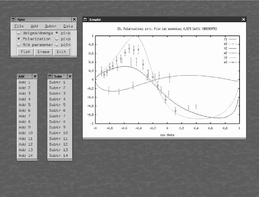
Figure 1: Screen shot of the plotting program. In the plot there are three different measurements at different momentum values ($0.192$ GeV/c, $0.425$ GeV/c and $0.573$ GeV/c ) [18, 19, 20], and the corresponding partial wave solutions — so it is possible to compare the goodness of the different data sets by the “eye ball” method. The scattered particles and the reaction can be chosen by the radiobutton widgets. The different data sets are selected by the same method as in the original code of Pietarinen, i.e. by moving up or down in the data base with Add or Sub buttons. The method is quite crude, and it is going to change when the data base is converted to MySQL format.

7.2 The current status

At present, the plotting program, the interpolation program and the program calculating the starting value of the fixed-$t$ analysis are ported to UNIX, and all the functionality of the original versions is implemented (fig. 1). The part, which iterates to adjust the fixed-$t$ amplitudes, the partial wave solution, and the experimental data, compiles OK but the GUI is still under construction. The heart of the whole program, the part making the actual analysis, is still in a completely untested stage.

7.3 Comparison of the numerics

We have compiled the code with different compilers running on different operating systems in order to check the stability of the mathematical subroutines. Comparing the results of the routines compiled by different compilers showed that the routines are not currently stable enough for production use.

For illustration, the interpolator part of the program calculates 173670 interpolated data points. When comparing the results of routines compiled by GNU Fortran to those calculated by NDP Fortran, one notices that 96% of the new data points agree up to 0.01%, but in some cases there are significant discrepancies: namely 73 data points of the 173670 differ by more than 1%, and in the worst case the difference is 28%. The cause of these discrepancies is unknown when writing this.

8 The next phase

After chasing the bugs and finding the reasons for the numerical unstabilities, we are hoping to find a better way to handle the propagation of the experimental errors than that used in the old KH analysis.

Because of the size of the data base, and because of the discrepancies in the different data sets, the visualisation of the data and the partial wave solutions is essential. Also, during the analysis, the program is used a lot, so the graphical user interface has to be easy and efficient to use. For making the choice of the data sets as easy as possible, we have plans to convert our text file data bases to MySQL format.

We intend to get the first preliminary results by the end of the year.

Acknowledgments:  We wish to thank A.M. Green for useful comments on the manuscript. We gratefully acknowledge financial support by the Academy of Finland grant 47678, the TMR EC-contract CT980169, and the Magnus Ehrnrooth foundation.

References

- [1] R. Koch and E. Pietarinen, Nucl. Phys. A336, 331 (1980).
- [2] G. van Rossum et al., http://www.python.org/ (1990-2001).
- [3] M. Widenius et al., http://www.mysql.com/.
- [4] M.M. Pavan et al., nucl-ex/0103006 (2001).
- [5] E. Frlež et al., Phys. Rev. C57, 3144 (1998), hep-ex/9712024.
- [6] M. Janousch et al, Phys. Lett. B414, 237 (1997).
- [7] C.V. Gaulard et al., Phys. Rev. C60, 024604 (1999).
- [8] G.J. Hofman et al., Phys. Rev. C58, 3484 (1998).
- [9] R. Wieser et al., Phys. Rev. C54, 1930 (1996).
- [10] I. Supek et al., Phys.Rev. D47, 1762 (1993).
- [11] B.J. Kriss et al., Phys. Rev. C59, 1480 (1999).
- [12] H.C. Schröder at al., Phys. Lett. B469, 25 (1999).
- [13] Ulf-G. Meißner, these proceedings, hep-ph/0108133 (2001).
- [14] G. Höhler, in: Landolt-Börnstein Vol. 9b2 (1983).
- [15] E. Pietarinen, Nucl. Phys. B107, 21 (1976).
- [16] E. Pietarinen, Physica Scripta 14, 11 (1976).
- [17] B. Tromborg, S. Waldenstrøm, and I. Øverbø, Phys.Rev. D15, 725 (1977).
- [18] J.C. Alder et al., Phys. Rev. D27, 1040 (1983).
- [19] J.C. Alder et al., Lett. Nuovo Cim. 23, 381 (1978).
- [20] V.S. Bekrenev et al., Sov. J. Nucl. Phys. 24, 45 (1976).