Mixing of meson, hybrid, and glueball states

The effective QCD Hamiltonian is constructed with the help of the background perturbation theory, and relativistic Feynman–Schwinger path integrals for Green’s functions. The resulting spectrum displays mass gaps of the order of one GeV, when additional valence gluon is added to the bound state.

Mixing between meson, hybrid, and glueball states is defined in two ways: through generalized Green’s functions and via modified Feynman diagram technic giving similar answers. Results for mixing matrix elements are numerically not large (around 0.1 GeV) and agree with earlier analytic estimates and lattice simulations.

1 Introduction

Gluonic fields play a double role in the dynamics of QCD. On one hand they create the QCD string between color charges which substantiates confinement. On another hand valence gluons act as color sources and can be considered as constituent pieces of hadrons on the same grounds as quarks. This is a QCD string picture of hybrids and glueballs developed analytically in [1] and confirmed by recent lattice calculations [2]. On experimental side the study of hybrid [3] and glueball [4] states is not yet conclusive, and more experimental and theoretical work is needed, especially a quantitative treatment of mixing between mesons, hybrids, and glueballs.

One typical feature of the QCD string approach, supported by lattice data [2], is that the addition of every valence gluon in a hadron increases the hadron mass by 0.8 – 1 GeV, and this is true also for purely gluonic states – glueballs. Thus a large mass gap exists between meson ground state and its gluonic excitation, which makes it possible to consider gluonic admixture in a given hadron state as a perturbation. Therefore in the zeroth approximation one has a Hamiltonian for the diagonal states of the fixed number of quarks $q,\bar{q}$ and valence gluons $g$, while in the next approximation one calculates the mixing between the states perturbatively (unless masses of the states happen to be almost degenerate, in which case one solves a matrix Hamiltonian).

The mixing between meson and hybrid states was considered previously analytically in [5, 6]. In [5] the hybrid wave function was taken in the cluster approximation, with gluon wave function of bag-model type factorized using the $q\bar{q}$ potential model wave function. The resulting mixing matrix elements (MME) are not large, supporting the iterative scheme described above. A similar approach, based on the nonrelativistic constituent quark and gluon model, was used in [6] to study mixing between $1^{-}c\bar{c}g$ hybrid meson and charmonium.

The mixing between glueballs and other hadrons was studied on the lattice [7], with reasonably moderate MME.

It is a purpose of the present paper to develop a general formalism of the QCD bound states including valence gluons, with the special attention to the mixing between states. This formalism is based on the QCD string approach [1] and applicable to both relativistic and nonrelativistic systems, massive or massless quarks and gluons.

Two features are important for this formalism. First, it is derived directly from QCD with few assumptions, supported and checked by lattice computations. Second, the only input of the theory is the fundamental string tension $\sigma_{f}$, current quark masses (renormalized at the scale of 1 GeV), and strong coupling constant $\alpha_{s}$. (For the total hadron masses one needs to subtract a selfenergy for each quark and antiquark equal to 0.25 GeV, but this does not affect wave functions and mixings which will be the main goal of this paper).

The plan of the paper is as follows. In the next section we develop the background perturbation theory to separate valence gluons from the background gluonic fields forming the QCD strings. On this basis the diagonal part of the QCD Hamiltonian is written for quarks, antiquarks, and valence gluons interacting via string connection and main characteristics of the spectrum are established for mesons, hybrids, and glueballs.

In section 3 the part of the Hamiltonian responsible for the mixing of mesons, hybrids, and glueballs is identified and MME is written in terms of solutions of the diagonal Hamiltonian, using formalism of modified plane waves.

In section 4 concrete calculations of MME are presented for meson-hybrid case based on the Green’s function formalism. An analogous treatment of the meson-glueball case is given in section 5.

In concluding section discussion is given of the results obtained in this paper and comparison is made with calculations with ohter model, lattice simulations, and experimental data.

2 Green’s functions and Hamiltonian

We follow in this section the procedure developed in detail in [9, 10] ( for earlier refs. see [11]) and therefore here we recapitulate only the main points. The total gluonic field $A_{\mu}$ is represented as a sum

$$A_{\mu}=B_{\mu}+a_{\mu},$$ (1)

where $B_{\mu}$ is the nonperturbative part and $a_{\mu}$ – perturbative (or valence gluon) part, which shall be treated in form of the perturbation series in $ga_{\mu}$. One can formally avoid the problem of doublecounting using the ’t Hooft identity, [9] which allows to represent the partition function as

$$Z=\frac{1}{N}\int e^{-S(A)}DqD\bar{q}DA=\frac{1}{N^{\prime}}\int\eta(B)e^{-S(B+a)}DBDaDqD\bar{q},$$ (2)

where $N,N^{\prime}$ are normalization constants.

Here $S$ is total Euclidean action and $\eta(B)$ – an arbitrary weight of averaging over $DB$. Expanding $S(B+a)$ one obtains

$$S(B+a)=S(B)+S_{1}(a,B)+S_{2}(a,B)+S_{3}(a,B)+S_{4}(a)+S_{1}(a,q,\bar{q})$$ (3)

In (3) $S_{n}(a,B)$ denotes terms of power $n$ in $a_{\mu}$, and $S_{1}(a,q,\bar{q})$ is the mixing term, which will be of main interest in section 3. The terms $S_{3}$ and $S_{4}$ contain additional powers of $g$ and can be treated perturbatively, the term $S_{1}(a,B)$ was considered in [10] and shown to yield a small correction to the leading terms $S(B)$ and $S_{2}(a,B)$, the latter defining the valence gluon propagating in the background $B_{\mu}$ with the Green’s function (in the background Feynman gauge [9]–[11])

$$G^{(g)}_{\mu\nu}=(D^{2}_{\lambda}\delta_{\mu\nu}+2igF_{\mu\nu})^{-1},~{}~{}D_{\lambda}=\partial_{\lambda}-igB_{\lambda},F_{\mu\nu}^{a}=\partial_{\mu}A_{\nu}^{a}-\partial_{\nu}A_{\mu}^{a}+gf^{abc}A_{\mu}^{b}A^{c}_{\nu}.$$ (4)

The explicit form of all terms in (3) and of the corresponding Green’s functions is given in [9, 10], here we only quote the results for the Green’s function of the state containing quark, antiquark, and any number of valence gluons in the leading $N_{c}$ approximation:

$$G_{q\bar{q}(ng)}(X,Y)\sim\langle\Gamma_{in}S_{q}(x,y)\prod^{n}_{i=1}G^{(g)}_{\mu_{i}\nu_{i}}(x,y)S_{\bar{q}}(x,y)\Gamma_{f}\rangle_{B}.$$ (5)

For (multi)glueball Green’s function one has a similar representation with missing factors $S_{q},S_{\bar{q}}$. Here $\Gamma_{in},\Gamma_{f}$ are initial and final vertex operators and $\langle...\rangle_{B}$ means averaging over fields $B_{\mu}$ with the weight $\eta(B)$, and quark Green’s function $S_{q}$ can be written as

$$S_{q}=-i(\hat{D}+m)^{-1}=-i(m-\hat{D})(m^{2}-\hat{D}^{2})^{-1}=-i(m-\hat{D})(m^{2}-\hat{D}^{2}_{\mu}-\sigma_{\mu\nu}F_{\mu\nu})^{-1}.$$ (6)

In what follows we shall treat spin-dependent terms for gluon and quark Green’s functions in (4) and (6) as a small correction, which is supported by exact calculations and comparison with experiment and lattice data [1]. Correspondingly one can use for the quadratic in $D_{\mu}$ parts the Feynman–Schwinger (world-line) path-integral representation (see [12, 13] and refs. therein)

$$(m^{2}-D^{2}_{\mu})_{xy}^{-1}=\int^{\infty}_{0}ds\int(Dz)_{xy}e^{-K}\exp(ig\int^{x}_{y}B_{\mu}dz_{\mu}),~{}~{}K=\frac{1}{4}\int^{s}_{0}(\frac{dz_{\mu}}{d\tau})^{2}d\tau.$$ (7)

It is important that background field $B_{\mu}$ enters (7) only in the exponentials and one can show [12] that in the total Green’s function (5) in the leading $N_{c}$ approximation all these exponentials combine into products of Wilson loops. Here we make another assumption, supported by lattice data, that Wilson loop has a minimal area law behaviour with the string tension $\sigma_{f}$ (for mesons and hybrids) and $\sigma_{\rm{adj}}=\frac{9}{4}\sigma_{f}$ for $2g$ glueballs. Thus one reduces the system of $q,\bar{q}$ and $n$ gluons to the open string with the ends at $q$ and $\bar{q}$, and $n$ gluons “sitting” on the string, and glueballs reduce to an open adjoint string (or equivalently for large $N_{c}$ – a closed fundamental string).

At this point one can define the Hamiltonian of the system $H$, using the relation for the general Green’s function of the type (5)

$$G(X,Y)=\langle X|\exp(-HT)|Y\rangle$$ (8)

where $T=X_{4}-Y_{4}$.

The Hamiltonian $H$ can be defined on any hyperplane, in case of center-of-mass system one gets the Hamiltonian which was obtained for the $q\bar{q}$ system in [14] and generalized in [17] to hybrid and in [16] to the glueball case (see also [15] for earlier papers on hybrid Hamiltonian).

Here we quote the simplest version of the Hamiltonian for $q\bar{q}$ and $n$ gluons, where string rotation contribution to the moment of inertia is treated as a perturbation:

$$H=H_{0}+\Delta H_{L}+\Delta H_{s}+\Delta H_{c}$$ (9)

where we have defined.

$$H_{0}=\frac{\mu_{q}+\mu_{\bar{q}}}{2}+\sum^{n}_{k=1}\frac{\mu_{k}}{2}+\sum_{k=q,\bar{q},1...n}\frac{\mbox{\boldmath${\rm p}$}^{2}_{k}+m^{2}_{k+1}}{2\mu_{k}}+\sigma_{f}\{|\mbox{\boldmath${\rm r}$}_{q}-\mbox{\boldmath${\rm r}$}_{1}|+|\mbox{\boldmath${\rm r}$}_{1}-\mbox{\boldmath${\rm r}$}_{2}|+...+|\mbox{\boldmath${\rm r}$}_{n}-\mbox{\boldmath${\rm r}$}_{\bar{q}}|\}.$$ (10)

Here $m_{k}=0$ for $k=1,...,n$ and $\mu_{k}$ defined as $\frac{1dz_{4}}{2d\tau_{k}}$ (see [14]) are to be found from the minimum of the $H_{0}$, which is approximated within 5% accuracy by the minimum of the eigenvalue $M_{0}^{(\nu)}$ [18], $H_{0}\Psi_{\nu}=M_{0}^{(\nu)}\Psi_{\nu}$:

$$\frac{\partial M_{0}^{(\nu)}}{\partial\mu_{k}}\left|{}_{\mu_{k}=\mu_{k}^{(0)}}\right.=0,~{}~{}k=q,\bar{q},1,...,n;\nu=0,1,2,...$$ (11)

$\Delta H_{L}$ gives zero contribution when all interparticle angular momenta are zero, and in particular for the meson case has the form [14]:

$$\Delta H_{L}=-\frac{16\sigma^{2}L(L+1)}{3M^{3}_{0}}.$$ (12)

The Coulombic part $\Delta H_{c}$ takes into account lowest-order Coulomb exchanges between quark and antiquark. It is argued in [16] that Coulomb exchanges between valence gluons are strongly suppressed by higher-loop corrections and hence can be neglected in the first approximation.

Finally, the spin-dependent term $\Delta H_{s}$ has the following form [1] for $q\bar{q}$ or $gg$ case

$$\Delta H_{s}=a\sum_{i,k=1,2}\frac{\mbox{\boldmath${\rm S}$}_{i}\cdot\mbox{\boldmath${\rm S}$}_{k}}{\mu_{i}\mu_{k}}+b_{1}\sum_{i}\frac{\mbox{\boldmath${\rm S}$}_{i}\cdot\mbox{\boldmath${\rm L}$}_{i}}{\mu_{i}^{2}}+\frac{b_{2}}{\mu_{1}\mu_{2}}\sum_{i}\mbox{\boldmath${\rm S}$}_{i}\cdot\mbox{\boldmath${\rm L}$}_{i}+c\frac{3(\mbox{\boldmath${\rm S}$}_{1}\cdot\mbox{\boldmath${\rm n}$})(\mbox{\boldmath${\rm S}$}_{2}\cdot\mbox{\boldmath${\rm n}$})-\mbox{\boldmath${\rm S}$}_{1}\cdot\mbox{\boldmath${\rm S}$}_{2}}{\mu_{1}\mu_{2}}.$$ (13)

In the c.m.s. $\mbox{\boldmath${\rm L}$}_{1}=-\mbox{\boldmath${\rm L}$}_{2}=\mbox{\boldmath${\rm L}$}$ $a,b_{1},b_{2}$, and $c$ depend on distance $r$ between $q\bar{q}(gg)$ and can be found in [1].

Let us now discuss the properties of the resulting Hamiltonian (9). First of all, one should stress that it is a fully relativistic Hamiltonian. Indeed, neglecting for the moment the interaction term in (10) and finding $\mu_{k}$ from (11) one immediately obtains $\mu_{k}=\sqrt{m^{2}_{k}+\mbox{\boldmath${\rm p}$}^{2}}$, i.e., in the free case $\mu_{k}$ plays the role of the relativistic energy of a quark or gluon. Moreover, the form of $\Delta H_{s}$ is not a result of expansion in inverse powers of large masses $\mu_{i},\mu_{k}$, but rather is a result of Gaussian approximation for the average of spin-dependent factors $\langle\prod_{n}\exp(g\sigma^{(n)}_{ik}F^{(n)}_{ik})\rangle_{B}$ (see [1] for details).

It is important to stress that $m_{q},m_{\bar{q}}$ entering the Hamiltonian (10) denote quark current masses, renormalized at the scale around 1GeV, and nowhere we use as input constituent masses of quarks or gluons.

The spectrum of the Hamiltonian (9) was calculated for many systems, including mesons, hybrids, and glueballs, for a review see [1]. As a recent example see calculation of gluelumps in [19].

The characteristic feature of the spectrum is that each constituent (quark or gluon) contributes to the total mass a quantity approximately equal to $2\mu^{(0)}_{k}$, where $\mu^{(0)}_{k}$ depends on the number of eigenvalue $\nu$ and is expressed through $\sigma_{f}$ (or $\sigma_{\rm adj}$ for glueballs). $\mu_{k}^{(0)}$ changes from 0.35 GeV for massless quarks in the lowest meson states, and $\sqrt{\frac{9}{4}}0.35=0.52$ GeV for gluons in the glueball. Therefore any gluon in a hybrid adds around 1 GeV to the total mass, and the same is true for glueballs: the lowest three-gluon glueball is approximately 1 GeV heavier than the lowest two-gluon glueball. This fact supports the idea outlined in the Introduction that the diagonal eigenvalues of the total Hamiltonian have energy gaps around 1 GeV and it may be a good approximation to treat mixing due to valence gluon excitation as a perturbation provided the MME is much less than 1 GeV.

3 Mixing matrix elements

We turn in this section to the part of interaction, $S_{1}(a,q,\bar{q})$, which is responsible for the mixing between hadronic states, differing by the number of valence gluons. It has the form

$$S_{1}(a,q,\bar{q})=g\int\bar{q}(x)\hat{a}(x)q(x)d^{4}x.$$ (14)

Here $\hat{a}(x)=a^{a}_{\mu}t^{a}_{\alpha\beta}\gamma_{\mu}$, and $\bar{q}_{\alpha},q_{\beta}$ all have color indices, whereas in the Hamiltonian (10) and its eigenfunctions the color indices are absent because of color averaging in $G_{q\bar{q}(ng)}$ (5) and hence in $H$.

To understand how the matrix element of $S_{1}$ is taken between colorless hadronic eigenfunctions of $H$, one can use the formalism of Green’s functions, described in Sections 4,5, and corresponding to the diagrams in Figs. 1–4.

Here we shall choose a simpler way, which leads to the same results as in sections 4,5, but more familiar for the reader accustomed to Feynman diagrams.

The rules are simple: represent each $q(x),\bar{q}(x)$ and $a_{\mu}(x)$ by equivalent colorless fields with familiar plane-wave expansion

$$q(\mbox{\boldmath${\rm x}$},t)=\sum_{\mbox{\boldmath${\rm k}$}}\frac{1}{\sqrt{2\mu_{q}(\mbox{\boldmath${\rm k}$})V}}[(u(k,\sigma)b_{\lambda}\exp({i\mbox{\boldmath${\rm k}$}\cdot\mbox{\boldmath${\rm x}$}-i\mu_{q}t})+u^{c}(k,\sigma)d_{\lambda}^{+}\exp({-i\mbox{\boldmath${\rm k}$}\cdot\mbox{\boldmath${\rm x}$}+i\mu_{q}t}))]$$ (15)

$$a_{\mu}(\mbox{\boldmath${\rm x}$},t)=\sum_{\mbox{\boldmath${\rm k}$},\lambda}\frac{1}{\sqrt{2\mu(\mbox{\boldmath${\rm k}$})V}}[\exp({i\mbox{\boldmath${\rm k}$}\cdot\mbox{\boldmath${\rm x}$}-i\mu t)}e^{(\lambda)}_{\mu}c_{\lambda}(\mbox{\boldmath${\rm k}$})+e^{(\lambda)}_{\mu}c^{+}_{\lambda}(\mbox{\boldmath${\rm k}$})\exp({-i\mbox{\boldmath${\rm k}$}\cdot\mbox{\boldmath${\rm x}$}+i\mu t})],$$ (16)

where $b_{\lambda}$ and $c_{\lambda}$ are annihilation operators for the quark and gluon respectively, $d^{+}_{\lambda}$ is creation operator for antiquark and $u(k)$ is normalized according to the condition $\bar{u}(k)u(k)=2\mu_{q}(k),$ $V$ - is the 3d volume and $e^{(\lambda)}_{\mu}$ is the gluon polarization vector.

One can easily check at this point that introduction of (16) into the free part of the QCD Hamiltonian $\frac{\mbox{\boldmath${\rm E}$}^{2}+\mbox{\boldmath${\rm B}$}^{2}}{2}$ immediately reproduces the gluonic part of the effective Hamiltonian (10) (the same is true for $q,\bar{q}$ if one uses the quadratic in ${\rm k}$ form of the Hamiltonian).

In (15), (16) $\mu_{q}(\mbox{\boldmath${\rm k}$})$ and $\mu(\mbox{\boldmath${\rm k}$})$ are the same quantities as in (10), to be defined by the minimization procedure in the system, where quark or gluon enter as constituents.

Another important point is the number of independent polarizations of a bound gluon. We shall use as in [9]–[11] ”the gauge-invariant gauge condition”

$$D_{\mu}a_{\mu}=0.$$ (17)

For a valence gluon in the gauge-invariant hybrid wave function $\Psi_{\mu}$ one has

$$\Psi_{\mu}(x,z,y)\equiv\bar{q}(x)\Phi(x,z)a_{\mu}(z)\Phi(z,y)q(y).$$ (18)

Here $\Phi$ are parallel transporters depending on $B_{\mu}$, $\Phi(x,y)=P\exp ig\int^{x}_{y}B_{\mu}dz_{\mu}$.

Differentiating $\Psi_{\mu}$ in $\frac{\partial}{\partial z_{\mu}}$ one obtains additional term $B_{\mu}$ due to differentiation of the end points in $\Phi(x,z),\Phi(z,y)$, so that one has

$$\frac{\partial}{\partial z_{\mu}}\Psi_{\mu}(x,z,y)=\bar{q}(x)\Phi(x,z)(D_{\mu}a_{\mu}(z))\Phi(z,y)q(y)+...$$ (19)

where dots imply the terms from the contour differentiation, i.e., due to additional gluonic excitation of the string.

In the diagonal approximation (and keeping in mind that gluonic excitation implies a gap of 1 GeV), we disregard those terms, and hence have the (approximate) condition

$$\frac{\partial}{\partial z_{\mu}}\Psi^{(h)}_{\mu}(x,z,y)=0.$$ (20)

This means that only 3 gluon polarizations are physical, i.e., the same situation as for an off-shell photon or gluon. In what follows we shall retain only
$\mu=1,2,3$. It is clear that the same reasoning applies to gluon in glueball.

We are now in the position to write the general form of wave functions for mesons, hybrids, and glueballs. In the momentum space and in the second-quantized form they can be written for a meson

$$\phi^{(M)}=f^{(\sigma_{1},\sigma_{2})}_{\alpha_{1},\alpha_{2}}(\mbox{\boldmath${\rm p}$}_{1},\mbox{\boldmath${\rm p}$}_{2})b^{+}_{\sigma_{1}}(p_{1})d_{\sigma_{2}}(p_{2}),$$ (21)

where $\sigma_{1},\sigma_{2}$ are polarizations (helicities) of $q$ and $\bar{q}$, and $\alpha_{1},\alpha_{2}$ are Dirac 4-spinor indices.

For a hybrid one has

$$\phi^{(H)}=f^{(\sigma_{1},\sigma_{2},\lambda)}_{\alpha_{1},\alpha_{2},\mu}(\mbox{\boldmath${\rm p}$}_{1},\mbox{\boldmath${\rm p}$}_{2},\mbox{\boldmath${\rm p}$}_{3})b^{+}_{\sigma_{1}}(p_{1})d_{\sigma_{2}}(p_{2})c^{+}_{\lambda}(p_{3})$$ (22)

where $\lambda$ is the gluon polarization and $\mu$ is discussed above, it enters as in $e^{(\lambda)}_{\mu}$ in (16). Finally for the glueball one has

$$\phi^{(G)}=f^{(\lambda_{1},\lambda_{2},)}_{\mu_{1},\mu_{2}}(\mbox{\boldmath${\rm p}$}_{1},\mbox{\boldmath${\rm p}$}_{2})c^{+}_{\lambda_{1}}(p_{1})c^{+}_{\lambda_{2}}(p_{2}).$$ (23)

One should note, that all wave functions (21)–(23) are given in the representation when the total angular momentum $J$ and its projection $M_{J}$ are not projected out. In fact the operator (21) is a 16 component structure, and one can use the classification introduced in [21] to distinguish positive and negative energy states of quarks using the so-called $\rho$-spin, $\rho=\pm$ and usual spin states for each quark. From spin and $\rho$-spin states one can construct the states with given total momentun and parity [22]. These scheme was exploited and developed in the series of papers [23] where the $q\bar{q}$ interaction was used containing both scalar and vector confining parts.

A similar scheme can be used for hybrids, but the resulting calculations are rather cumbersome. Therefore in this section we only list some schematic expressions with coefficients for mesons which can be found in [23] and for hybrids not yet available (to the knowledge of the author). Thus one can write instead of wave functions (21)–(23) the functions $\Phi^{(M)}_{J},\Phi^{(H)}_{J}$, and $\Phi^{(G)}_{J}$ with given total angular momentum. Each of this functions consists of several components differing in total spin, orbital momentum, and $\rho$-spins. It is actually those combinations which should be inserted everywhere below in this chapter instead of $\Phi^{(M)},\Phi^{(H)}$, and $\Phi^{(G)}$, respectively, but we keep for simplicity reason the functions (21)–(23), referring the reader to the Appendix for more details and discussion.

We are now in position to write down the MME between states (21)–(23), using the interaction Hamiltonian, obtained from (14), namely

$$H_{1}=g\int\bar{q}(\mbox{\boldmath${\rm x}$},0)\hat{a}(\mbox{\boldmath${\rm x}$},0)q(\mbox{\boldmath${\rm x}$},0)d^{3}x=$$

$$=g\sum_{\mbox{\boldmath${\rm k}$}_{1},\mbox{\boldmath${\rm k}$}_{2},\mbox{\boldmath${\rm k}$}_{3}}\bar{q}(\mbox{\boldmath${\rm k}$}_{1})\hat{a}(\mbox{\boldmath${\rm k}$}_{3})q(\mbox{\boldmath${\rm k}$}_{2})\frac{d^{3}k_{1}}{(2\pi)^{3}}\frac{d^{3}k_{2}}{(2\pi)^{3}}\frac{d^{3}k_{3}}{(2\pi)^{3}}{(2\pi)^{3}}\delta^{(3)}(\mbox{\boldmath${\rm k}$}_{1}+\mbox{\boldmath${\rm k}$}_{2}+\mbox{\boldmath${\rm k}$}_{3}).$$ (24)

For the meson-hybrid mixing one has

$$(\Phi^{(M)},H_{1}\Phi^{(H)})=g\int f^{+(\sigma_{1},\sigma_{2})}_{\alpha_{1},\alpha_{2}}(\mbox{\boldmath${\rm p}$}_{1},\mbox{\boldmath${\rm p}$}_{2})\frac{\hat{e}^{(\lambda)}(k_{3})}{\sqrt{2\mu(k_{3})}}f^{\sigma^{\prime}_{1},\sigma^{\prime}_{2},\lambda}_{\alpha^{\prime}_{1},\alpha_{2},\mu}(\mbox{\boldmath${\rm p}$}^{\prime}_{1},\mbox{\boldmath${\rm p}$}_{2},\mbox{\boldmath${\rm k}$}_{3})\times$$

$$\times\frac{d\mbox{\boldmath${\rm p}$}_{1}}{(2\pi)^{3}}\frac{d\mbox{\boldmath${\rm p}$}^{\prime}_{1}}{(2\pi)^{3}}\frac{d\mbox{\boldmath${\rm k}$}_{3}}{(2\pi)^{3}}\delta^{(3)}(-\mbox{\boldmath${\rm p}$}_{1}+\mbox{\boldmath${\rm p}$}^{\prime}_{1}+\mbox{\boldmath${\rm k}$}_{3})(2\pi)^{3}\frac{d^{3}p_{2}}{(2\pi)^{3}}(2\pi)^{3}\delta^{(3)}(\mbox{\boldmath${\rm p}$}_{1}+\mbox{\boldmath${\rm p}$}_{2}).$$ (25)

The normalization condition for $\Phi^{(M)},\Phi^{(H)}$ looks like

$$(\Phi^{(M)},\Phi^{(M)})=\int f^{+(\sigma_{1},\sigma_{2})}_{\alpha_{1},\alpha_{2}}(\mbox{\boldmath${\rm p}$}_{1},\mbox{\boldmath${\rm p}$}_{2})f^{(\sigma^{\prime}_{1},\sigma^{\prime}_{2})}_{\alpha_{1},\alpha_{2}}(\mbox{\boldmath${\rm p}$}_{1},\mbox{\boldmath${\rm p}$}_{2})dP_{2}=\delta_{\sigma_{1}\sigma^{\prime}_{1}}\delta_{\sigma_{2}\sigma^{\prime}_{2}},$$ (26)

$$(\Phi^{(H)},\Phi^{(H)})=\int f^{+(\sigma_{1},\sigma_{2},\lambda)}_{\alpha_{1},\alpha_{2},\mu}(\mbox{\boldmath${\rm p}$}_{1},\mbox{\boldmath${\rm p}$}_{2},\mbox{\boldmath${\rm p}$}_{3})f^{(\sigma^{\prime}_{1},\sigma^{\prime}_{2},\lambda^{\prime})}_{\alpha_{1},\alpha_{2},\mu}(\mbox{\boldmath${\rm p}$}_{1},\mbox{\boldmath${\rm p}$}_{2},\mbox{\boldmath${\rm p}$}_{3})dP_{3}=\delta_{\sigma_{1}\sigma^{\prime}_{1}}\delta_{\sigma_{2}\sigma^{\prime}_{2}}\delta_{\lambda\lambda^{\prime}},$$ (27)

where we have defined

$$dP_{3}\equiv\prod^{3}_{i=1}\frac{d^{3}\mbox{\boldmath${\rm p}$}_{i}}{(2\pi)^{3}}(2\pi)^{3}\delta^{(3)}(\mbox{\boldmath${\rm p}$}_{1}+\mbox{\boldmath${\rm p}$}_{2}+\mbox{\boldmath${\rm p}$}_{3}),$$ (28)

$$dP_{2}\equiv\prod^{2}_{i=1}\frac{d^{3}\mbox{\boldmath${\rm p}$}_{i}}{(2\pi)^{3}}(2\pi)^{3}\delta^{(3)}(\mbox{\boldmath${\rm p}$}_{1}+\mbox{\boldmath${\rm p}$}_{2}).$$ (29)

Going from momentum to coordinate representation and suppressing for the moment the momentum dependence of the factor $\Gamma(p_{1},p^{\prime}_{1},k_{3})$ in (25), where

$$\Gamma(p_{1},p^{\prime}_{1},k_{3})\equiv\frac{\hat{e}^{(\lambda)}(k_{3})}{\sqrt{2\mu(k_{3})}},$$ (30)

one has

$$(\Phi^{(M)},H_{1}\Phi^{(H)})=g\int d^{3}\mbox{\boldmath${\rm r}$}\varphi^{(M)}(\mbox{\boldmath${\rm r}$})\Gamma\varphi^{(H)}(0,\mbox{\boldmath${\rm r}$})$$ (31)

where we have defined

$$\varphi^{(M)}(\mbox{\boldmath${\rm r}$})\equiv\int f^{(\sigma_{1},\sigma_{2})}_{\alpha_{1},\alpha_{2}}(\mbox{\boldmath${\rm p}$}_{1},\mbox{\boldmath${\rm p}$}_{2})e^{i\mbox{\boldmath${\rm p}$}_{1}\cdot\mbox{\boldmath${\rm r}$}_{1}+i\mbox{\boldmath${\rm p}$}_{2}\cdot\mbox{\boldmath${\rm r}$}_{2}}dP_{2}=$$

$$=\int f^{(\sigma_{1},\sigma_{2})}_{\alpha_{1},\alpha_{2}}(\mbox{\boldmath${\rm p}$}_{1},-\mbox{\boldmath${\rm p}$}_{1})e^{i\mbox{\boldmath${\rm p}$}_{1}\cdot\mbox{\boldmath${\rm r}$}_{1}}\frac{d\mbox{\boldmath${\rm p}$}_{1}}{(2\pi)^{2}},~{}~{}\mbox{\boldmath${\rm r}$}=\mbox{\boldmath${\rm r}$}_{1}-\mbox{\boldmath${\rm r}$}_{2};$$ (32)

$$\varphi^{(H)}(0,\mbox{\boldmath${\rm r}$})=\int f^{(\sigma_{1},\sigma_{2},\lambda)}_{\alpha_{1},\alpha_{2},\mu}(\mbox{\boldmath${\rm p}$}_{1},\mbox{\boldmath${\rm p}$}_{2},\mbox{\boldmath${\rm p}$}_{3})e^{i\mbox{\boldmath${\rm p}$}_{1}\cdot\mbox{\boldmath${\rm r}$}_{1}+i\mbox{\boldmath${\rm p}$}_{2}\cdot\mbox{\boldmath${\rm r}$}_{2}+i\mbox{\boldmath${\rm p}$}_{3}\cdot\mbox{\boldmath${\rm r}$}_{3}}dP_{3}$$ (33)

with $\mbox{\boldmath${\rm r}$}_{1}-\mbox{\boldmath${\rm r}$}_{3}=0,~{}~{}\mbox{\boldmath${\rm r}$}_{1}-\mbox{\boldmath${\rm r}$}_{2}\equiv\mbox{\boldmath${\rm r}$}.$

In the next two sections we shall use another formalism to derive MME – the formalism of Green’s functions, which enables us to use our Hamiltonian technic described in chapter 2.

4 Mixing between meson and hybrid states

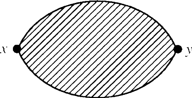
Figure 1: Meson Green’s function describing propagation of the quark and antiquark (solid lines) from the point $x$ to the point $y$. The hatched interior of the figure implies presence of nonperturbative fields $B_{\mu}$ in the form of the fundamental string world sheet.

Consider a nonsinglet $q\bar{q}$ state; the corresponding Green’s function in the quenched (large $N_{c}$) approximation can be written, according to general formulas [12, 13], as (see Fig. 1 for the corresponding Feynman diagram)

$$G_{q\bar{q}}(x,y)=\langle\bar{\psi}(x)\Gamma^{({\rm out})}\psi(x)\bar{\psi}(y)\Gamma^{({\rm in})}\psi(y)\rangle_{B,a,\psi,\bar{\psi}}=$$

$$=\langle tr\Gamma^{({\rm out})}S(x,y)\Gamma^{({\rm in})}S(y,x)\rangle_{B,a}.$$ (34)

Here averaging over $B,a$ is assumed with the action given in (2),(3) and $S(x,y)$ is the quark Green’s function,

$$S(x,y)=-i(\hat{D}+m)^{-1}_{x,y},D_{\mu}=\partial_{\mu}-igB_{\mu}.$$ (35)

Writing $S=-i(m-\hat{D})(m^{2}-\hat{D}^{2})^{-1}$, one can reduce the Wilson-loop path integral for $G_{q\bar{q}}$ to the form

$$G_{q\bar{q}}(x,y)=\langle tr_{c\alpha}\Gamma^{({\rm out})}(m-\hat{D})\int^{\infty}_{0}\int^{\infty}_{0}dsd\bar{s}e^{-K-\bar{K}}(Dz)_{xy}(D\bar{z})_{xy}\Gamma^{({\rm in})}(\bar{m}-\hat{\bar{D}})W_{F}\rangle.$$ (36)

Here $W_{F}$ is the Wilson loop with insertion of operators $\sigma F$, defined in [6], and trace is over color (c) and Lorentz $(\alpha)$ indices.

Our primary task now is to transform the integral $\int ds(Dz)_{xy}$ of each quark Green’s function as follows:

$$ds(Dz)_{xy}=ds\prod^{N}_{n=1}\frac{d^{4}z(n)}{(4\pi\varepsilon)^{2}}\frac{d^{4}p}{(2\pi)^{4}}e^{ip(x-y-\sum_{n}z(n))},~{}~{}N\varepsilon=s.$$ (37)

Introducing now the parameter $\mu(z_{4})$ playing the role of constituent quark mass according to

$$ds=\frac{dz_{4}}{2\mu(z_{4})},~{}~{}\int ds\frac{dp_{4}}{2\pi}e^{ip_{4}(\sum_{n}\Delta z_{4}^{(n)}-T)}=\int ds\delta(2\bar{\mu}s-T)=\frac{1}{2\bar{\mu}},$$

where $2\bar{\mu}s=\sum_{n}\Delta z_{4}(n)=\sum_{n}\Delta s2\mu(n)$, one obtains

$$Ds(Dz)_{xy}=\frac{1}{2\bar{\mu}}\frac{d^{3}p}{(2\pi)^{3}}e^{i\mbox{\boldmath${\rm p}$}\cdot(\mbox{\boldmath${\rm x}$}-\mbox{\boldmath${\rm y}$}-\sum_{n}\mbox{\boldmath${\rm z}$}(n))}D^{3}zD\mu.$$ (38)

Thus the path integral for each Green’s function acquires the 3-d form, which we call $G_{(3d)}$, with all Zitterbewegung ($z$-graphs) contained in the integral over $D\mu$. If one does, as we usually do for all systems (except pion and kaon), the stationary point procedure in integration over $D\mu$, then one finds the smooth ”constituent mass trajectory” $\mu_{0}(t)(t\equiv z_{4})$, or a simple approximation to it, the constant constituent mass $\bar{\mu}_{0}$, found from the minimum of the Hamiltonian eigenvalue [20]. In this approximation (yielding accuracy around 5% for masses [18]) one can identify $\bar{\mu}$ in (38) and $\bar{\mu}_{0}$.

Thus one can write

$$S(x,y)=\frac{m-\hat{D}}{2\bar{\mu}_{q}}G_{3d}(x,y)=\frac{m-\hat{D}}{2\bar{\mu}_{q}}\langle x|n\rangle e^{-M_{n}|x-y|}\langle n|y\rangle,$$ (39)

where $M_{n}$ is the n-th eigenvalue of the Hamiltonian. Similarly for the gluon Green’s function one writes

$$G_{\mu\nu}(x,y)=(-\hat{D}^{2}\delta_{\mu\nu}-2i\hat{F}_{\mu\nu})^{-1}_{xy}=\frac{1}{2\bar{\mu}_{g}}\langle x,\mu|n\rangle e^{-M_{n}|x-y|}\langle n|y,\nu\rangle.$$ (40)

The form in (39),(40) is highly symbolic, since quarks and gluons do not propagate separately (and do not have separate eigenfunctions $(|n\rangle)$, but rather form the common bound state. In the free case one can identify $\bar{\mu}_{q}$ with the energy $E_{q},\bar{\mu}_{g}$ with $\omega_{g}$, and $|n\rangle=\frac{\exp({i\mbox{\boldmath${\rm p}$}\cdot\mbox{\boldmath${\rm x}$}})}{(2\pi)^{3/2}}$, so that (39), (40) go over into well-known representation

$$S(x,y)=-i(m-\hat{\partial})\int\frac{d^{3}p}{(2\pi)^{3}}\frac{\exp({i\mbox{\boldmath${\rm p}$}\cdot\mbox{\boldmath${\rm x}$}-E|x_{4}-y_{4}|)}}{2E(p)},$$ (41)

$$G_{\mu\nu}(x,y)=\delta_{\mu\nu}\int\frac{d^{3}\mbox{\boldmath${\rm k}$}\exp({i(\mbox{\boldmath${\rm k}$}\cdot\mbox{\boldmath${\rm x}$}-\omega|x_{4}-y_{4}|)})}{(2\pi)^{3}2\omega(k)}.$$ (42)

Consider now the hybrid Green’s function

$$G^{(h)}(x^{(1)},x^{(2)},x^{(3)}|(y^{(1)},y^{(2)},y^{(3)})=\langle\Psi^{(h)+}(x^{(1)},x^{(2)},x^{(3)})\Psi^{(h)}(y^{(1)},y^{(2)},y^{(3)})\rangle_{B,a,q}.$$ (43)

Omitting parallel transporters for simplicity, one can write

$$G^{(h)}=\sum^{\infty}_{n=0}\langle\mbox{\boldmath${\rm x}$}^{(1)},\mbox{\boldmath${\rm x}$}^{(2)},\mbox{\boldmath${\rm x}$}^{(3)}|n\rangle\Lambda_{q}^{(1)}\Lambda^{(2)}_{\bar{q}}\frac{e^{-M_{n}T}}{2\bar{\mu}_{g}(n)}\langle n|\mbox{\boldmath${\rm y}$}^{(1)},\mbox{\boldmath${\rm y}$}^{(2)},\mbox{\boldmath${\rm y}$}^{(3)}\rangle,$$ (44)

where we have denoted $\Lambda_{q}^{(1,2)}=\frac{m-\hat{D}}{2\bar{\mu}_{q}}$ for quark and antiquark respectively.

The Hamiltonian eigenfunctions $\langle n|\mbox{\boldmath${\rm y}$}^{(1)},\mbox{\boldmath${\rm y}$}^{(2)},\mbox{\boldmath${\rm y}$}^{(3)}\rangle$ are characterized by the c.m. momentum ${\rm P}$, and boundstate quantum numbers $n$ and the sum over $n$ in (44) can be written as

$$\int\frac{d^{3}\mbox{\boldmath${\rm P}$}e^{i\mbox{\boldmath${\rm P}$}\cdot(\mbox{\boldmath${\rm X}$}-\mbox{\boldmath${\rm Y}$})}}{(2\pi)^{3}2\bar{\mu}_{g}(n)}\varphi^{+}_{n}(\mbox{\boldmath${\rm\xi}$}^{(1)},\mbox{\boldmath${\rm\xi}$}^{(2)})\varphi_{n}(\mbox{\boldmath${\rm\eta}$}^{(1)},\mbox{\boldmath${\rm\eta}$}^{(2)})$$ (45)

where $\mbox{\boldmath${\rm\xi}$}^{(i)};\mbox{\boldmath${\rm\eta}$}^{(i)}$ are Jacobi coordinates, while $\mbox{\boldmath${\rm X}$},\mbox{\boldmath${\rm Y}$}$ are c.m. coordinates.

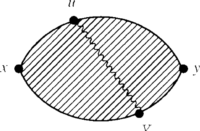
Figure 2: The same as in Fig.1 but with one perturbative gluon passing between points $u$ and $v$ described by a wavy line.

We are now in the position to write the amplitude, corresponding to the Feynman diagram of Fig.2, where the valence gluon $a_{\mu}$ is emitted at the point $u$ and absorbed at the point $v$. The corresponding term in the Lagrangian is given in (14),

$$S_{1}(a,q,\bar{q})=\int\bar{q}(x)g\hat{a}(x)q(x)d^{4}x.$$ (46)

The general form of the amplitude of Fig.2 is

$$G_{q\bar{q}}^{(2)}=\int\langle{\rm tr}_{C\alpha}\Gamma^{({\rm out})}S(x,u)t^{a}g\gamma_{\mu}d^{4}uS(u,y)G^{ab}_{\mu\nu}(u,v)\Gamma^{({\rm in})}\times$$

$$\times S(y,v)g\gamma_{\nu}t^{b}d^{4}vS(v,x)\rangle_{B}.$$ (47)

Here trace is over both color $(c)$ and Lorentz $(\alpha)$ indices.

Introducing now the representations as in (44), (45), one obtains finally

$$G_{q\bar{q}}^{(2)}=\frac{N^{2}_{c}{\rm tr}_{\alpha}}{2}\langle\Lambda_{q}\Gamma^{(out)}\Lambda_{\bar{q}}\varphi^{+}_{M}(0)\int\sum_{n}\frac{\gamma_{\mu}V_{Mn}^{(\mu)}V_{nM}^{(\nu)}\gamma_{\nu}\varphi_{M}(0)\Lambda_{q}\Gamma^{(in)}\Lambda_{\bar{q}}\rangle}{2\mu_{g}(n)(M_{h}^{(n)}-M_{M})(M_{M}-M_{h}^{(n)})}\times$$

$$\times\frac{d^{3}\mbox{\boldmath${\rm P}$}}{(2\pi)^{3}}e^{i\mbox{\boldmath${\rm P}$}\cdot(\mbox{\boldmath${\rm x}$}-\mbox{\boldmath${\rm y}$})-E_{M}(y_{4}-x_{4})}.$$ (48)

Here notations are used

$$V_{Mn}^{(\mu)}=g\int\varphi_{M}(\mbox{\boldmath${\rm r}$})^{\mu}\psi^{+}_{n}(0,\mbox{\boldmath${\rm r}$})d^{3}\mbox{\boldmath${\rm r}$}$$ (49)

and $\varphi_{M}(\mbox{\boldmath${\rm r}$})$ , ${}^{\mu}\psi_{n}$ are meson and hybrid eigenfunctions respectively (with the gluon in the latter having polarization $\mu$), while $M_{M},M_{h}^{(n)}$ are masses of the meson and hybrid (in the $n$-th excited state) respectively. Note that while $G_{q\bar{q}}$ (36) is $O(N_{c})$ due to ${\rm tr}_{c}$, $G_{q\bar{q}}^{(2)}$ is $O(g^{2}N^{2}_{c})=O(N_{c})$, since gluon line in Fig.2 is equivalent to double fundamental line, yielding two color traces in Fig.2.

From (48) one can see that the basic element defining the amplitude of the mixing of meson and hybrid is the dimensionless ratio

$$\frac{V_{on}^{(\mu)}}{\sqrt{2\mu_{g}(n)}|M_{h}^{(n)}-M_{M}|}\equiv\lambda_{n}^{MH}$$ (50)

The rest of this section is devoted to the calculation of the matrix element $V_{Mn}^{(\mu)}$ using realistic wave functions for the meson and hybrid.

To make estimates of $V_{Mn}$, we first remark that to the lowest approximation in spin splittings both $\varphi_{M}$ and ${}^{\mu}\psi_{n}$ are proportional to unit matrices in Lorentz indices, and moreover the gluon Green’s function $G^{ab}_{\mu\nu}$ is proportional to $\delta_{\mu\nu}$, where each bound gluon acquires its mass due to the attached string (similarly to the $W^{\pm},Z^{0}$ acquiring mass due to attached Higgs condensate) and hence the sum over $\mu\nu$ is the sum over 3 polarizations.

As a result $V_{Mn}^{(\mu)}V_{nM}^{(\nu)}\sim\delta_{\mu\nu}$ and ${}^{\mu}\psi^{+}_{n}(0,\mbox{\boldmath${\rm r}$})$ does not depend on $\mu$ in the same lowest approximation (when gluon spin contribution to the hybrid mass is neglected; both for mesons and hybrids the spin splitting is less or about 10% of the total energy and our estimates will have this accuracy).

The meson wave function $\varphi_{M}(\mbox{\boldmath${\rm r}$})$ for linear growing potential is Airy function, for our purposes it is enough to use a Gaussian with the proper radius $r_{0}$, e.g.

$$\varphi_{M}(r)=\left(\frac{3}{2r^{2}_{0}\pi}\right)^{3/4}e^{-\frac{3}{4}\left(\frac{r}{r_{0}}\right)^{2}}.$$ (51)

Using $r_{0}$ as a variational parameter, one gets

$$\langle r^{2}\rangle=r^{2}_{0}=0.725{\rm fm}^{2}.$$ (52)

For the hybrid wave function one can use the eigenfunction of the Hamiltonian (10) in the lowest hyperspherical approximation, where for an estimate we approximate $W(\rho)$ by the oscillator well $C(\rho-\rho_{0})^{2},C\equiv\frac{m\omega^{2}}{2}$ near its minimal value (the accuracy of this procedure is around one percent for the cases considered, see [24])).

Then one can write

$$\psi(\mbox{\boldmath${\rm r}$}_{13},\mbox{\boldmath${\rm r}$}_{32})=\frac{1}{\rho^{5/2}\sqrt{\Omega_{6}}}\left|\det\left(\begin{array}[]{lll}\mbox{\boldmath${\rm r}$}_{1}&\mbox{\boldmath${\rm r}$}_{2}&\mbox{\boldmath${\rm r}$}_{3}\\ \mbox{\boldmath${\rm R}$}&\mbox{\boldmath${\rm\xi}$}&\mbox{\boldmath${\rm\eta}$}\end{array}\right)\right|^{1/2}\left(\frac{m\omega}{\pi}\right)^{1/4}e^{-\frac{m\omega}{2}(\rho-\rho_{0})^{2}}.$$ (53)

Here $m$ is an arbitrary mass, used for dimensional reasons and disappearing from final answers, $\rho_{0}$ is found from the minimum of $W(\rho)$, $W^{\prime}(\rho=\rho_{0})=0$, and $w$ is expressed through $W^{{}^{\prime\prime}}(\rho_{0}),m\omega^{2}=W^{{}^{\prime\prime}}(\rho_{0})$, so that

$$\omega=(1.358)^{2/3}\sqrt{3}\sigma^{2/3}\left(\frac{\mu_{1}+\mu_{3}}{\mu_{1}\mu_{3}}\right)^{1/3}\frac{1}{[{\cal L}({\cal{L}}+1)]^{1/6}},{\cal L}=K+\frac{3}{2},$$ (54)

$$\rho_{0}=\frac{2}{\sqrt{m}}\left(\frac{{\cal L}({\cal L}+1)}{1.358\sigma}\right)^{1/3}\left(\frac{\mu_{1}\mu_{3}}{\mu_{1}+\mu_{3}}\right)^{1/6},$$ (55)

$$\left|\det\left(\begin{array}[]{lll}\mbox{\boldmath${\rm r}$}_{1}&\mbox{\boldmath${\rm r}$}_{2}&\mbox{\boldmath${\rm r}$}_{3}\\ \mbox{\boldmath${\rm R}$}&\mbox{\boldmath${\rm\xi}$}&\mbox{\boldmath${\rm\eta}$}\end{array}\right)\right|^{1/2}=\left(\frac{\mu_{1}\mu_{2}\mu_{3}}{\mu m^{2}}\right)^{3/4},~{}~{}~{}\mu=\mu_{1}+\mu_{2}+\mu_{3}.$$ (56)

The determinant (56) appears due to the change of variables, as follows:

$$\int d\mbox{\boldmath${\rm r}$}_{1}d\mbox{\boldmath${\rm r}$}_{2}d\mbox{\boldmath${\rm r}$}_{3}|\Psi|^{2}=\int d\mbox{\boldmath${\rm R}$}d\mbox{\boldmath${\rm\xi}$}d\mbox{\boldmath${\rm\eta}$}|\psi|^{2}|\det()|=\int d\mbox{\boldmath${\rm R}$}\rho^{5}d\rho d\Omega_{6}|\Psi|^{2}|\det()|.$$ (57)

Finally $\int d\Omega_{6}\equiv\Omega_{6}=\pi^{3}$ and we need expression of $\rho$ through $\mbox{\boldmath${\rm r}$}_{13},\mbox{\boldmath${\rm r}$}_{23}$ etc., namely

$$\rho^{2}=\mbox{\boldmath${\rm\eta}$}^{2}+\mbox{\boldmath${\rm\xi}$}^{2}=\sum_{i<j}\frac{\mu_{i}\mu_{j}}{m\mu}(\mbox{\boldmath${\rm r}$}_{i}-\mbox{\boldmath${\rm r}$}_{j})^{2}.$$ (58)

In $V_{Mn}$ enters $\Psi_{n}$ at $\mbox{\boldmath${\rm r}$}_{13}=0,\mbox{\boldmath${\rm r}$}_{23}=\mbox{\boldmath${\rm r}$}_{21}\equiv\mbox{\boldmath${\rm r}$},$ which yields

$$\rho^{2}=\mbox{\boldmath${\rm r}$}^{2}\frac{\mu_{1}(\mu_{3}+\mu)}{2m\mu}.$$ (59)

Insertion of (51)–(56) in (48) yields

$$\frac{V_{Mn}}{\sqrt{2\mu_{g}}}=Cg\frac{r_{0}^{3/2}\sigma\mu_{1}J}{\sqrt{2\mu_{g}}}$$ (60)

where following notations are used:

$$J=\int^{\infty}_{0}t^{2}dte^{-t^{2}-a(t-b)^{2}},$$ (61)

$$C=\frac{1.358\cdot 2^{17/4}}{\pi^{4}({\cal L}({\cal L}+1))^{7/8}3^{5/8}}\left(\frac{\mu_{1}+\mu_{3}}{\mu_{3}}\right)^{1/2}\left(\frac{\mu_{3}}{\mu}\right)^{3/4},$$ (62)

$$a=\frac{2\omega r_{0}^{2}}{3}\frac{\mu_{1}(\mu_{1}+\mu_{3})}{\mu},~{}~{}b=\rho_{0}\sqrt{\frac{3\mu m}{4r^{2}_{0}\mu_{1}(\mu_{1}+\mu_{3})}}.$$ (63)

In (60) $\mu_{g}$ is the gluon effective energy, where gluon belongs to the hybrid, so that $\mu_{g}=\mu_{3}$.

We can do now estimates of $V_{Mon}$ both for light and heavy quarks. Using [20, 1] for massless quarks and for $\sigma=0.18$ GeV² one has $\mu_{2}=\mu_{1}=0.312$ GeV, $\mu_{3}=0.442$ GeV.  $\omega=0.956$ GeV, $a=2.54,~{}~{}b=0.813,$ and hence

$$\frac{V_{Mn}}{\sqrt{2\mu_{3}}}=g\cdot 0.2J\mathrel{\mathchoice{\lower 3.6pt\vbox{\halign{$\mathsurround=0pt\displaystyle\hfil#\hfil$\cr<\crcr\sim\crcr}}}{\lower 3.6pt\vbox{\halign{$\mathsurround=0pt\textstyle\hfil#\hfil$\cr<\crcr\sim\crcr}}}{\lower 3.6pt\vbox{\halign{$\mathsurround=0pt\scriptstyle\hfil#\hfil$\cr<\crcr\sim\crcr}}}{\lower 3.6pt\vbox{\halign{$\mathsurround=0pt\scriptscriptstyle\hfil#\hfil$\cr<\crcr\sim\crcr}}}}g\cdot 0.08~{}{\rm GeV}.$$ (64)

For heavy quarks, e.g., for $m_{1}=m_{2}=4.8$ GeV, one has $r_{0}=0.356$ fm, $\mu_{1}\simeq m_{1}=4.8$ GeV, $\mu_{3}=0.767$ GeV, and $\omega=0.5$ GeV. Inserting all these values in (60) one obtains again for heavy meson-heavy hybrid mixing

$$\frac{V_{Mn}}{\sqrt{2\mu_{3}}}=g\cdot 0.08~{}{\rm GeV}.$$ (65)

This estimate is close to the calculations made in [5, 6]. Hence one obtains a small mixing parameter $\lambda_{n}$ in (50) when mass difference between meson and hybrid is large, $\Delta\sim 1$ GeV, namely

$$\lambda_{n}\mathrel{\mathchoice{\lower 3.6pt\vbox{\halign{$\mathsurround=0pt\displaystyle\hfil#\hfil$\cr<\crcr\sim\crcr}}}{\lower 3.6pt\vbox{\halign{$\mathsurround=0pt\textstyle\hfil#\hfil$\cr<\crcr\sim\crcr}}}{\lower 3.6pt\vbox{\halign{$\mathsurround=0pt\scriptstyle\hfil#\hfil$\cr<\crcr\sim\crcr}}}{\lower 3.6pt\vbox{\halign{$\mathsurround=0pt\scriptscriptstyle\hfil#\hfil$\cr<\crcr\sim\crcr}}}}0.1g$$ (66)

while for close values of meson and hybrid masses, $\Delta M\sim 0.1$ GeV, the mixing can be large and one should use the many-channel Hamiltonian, which can be obtained from (10).

5 Mixing of glueball with hybrid and mesons

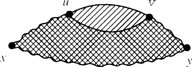
Figure 3: Glueball Green’s function describing propagation of two gluons (wavy lines) from point $x$ to point $y$, with insertion of quark-antiquark propagators (solid lines) from point $u$ to point $v$. The cross-hatched region refers to the adjoint string world sheet, while hatched region between quark lines has the same meaning as in Fig. 1.

Here we consider a two-gluon glueball state, and using the same methods as discussed in Section 4 and Sections 1,2 we write the amplitude corresponding to the diagram of Fig.3:

$$G_{gg}^{(2)\mu\nu,\mu^{\prime}\nu^{\prime}}(x,y)\equiv g^{2}{\rm tr}_{c}\{\Gamma^{({\rm out})}G_{\mu\rho}(x,u)t^{a}{\rm tr}_{\alpha}(\gamma_{\rho}S(u,v)\gamma_{\sigma}S(v,u))\times$$

$$\times t^{b}G_{\sigma\nu}(v,y)\Gamma^{({\rm in})}G_{\mu^{\prime}\nu^{\prime}}(x,y)\}.$$ (67)

Representing each gluon line at large $N_{c}$ as a double fundamental line, one gets two closed color contours in Fig.3 and as a result the factor $N_{c}^{2}$, hence the amplitude of Fig. 3 is $O(g^{2}N_{c}^{2})\sim O(N_{c})$ as well as the leading two-gluon diagram $G_{gg}^{(0)}$ which means that mixing here also appears in the leading order of the $1/N_{c}$ expansion.

Using expressions for the Green’s functions (39), (40), one obtains that insertion of the quark loop in Fig. 3 contributes to the glueball Green’s function the term

$$G_{gg}^{(2)\mu\nu,\mu^{\prime}\nu^{\prime}}=\frac{N_{c}^{2}}{2}{\rm tr}_{\alpha}\{\Gamma^{({\rm out})}\varphi^{+(\mu\nu)}_{G}(0)\sum_{n}\frac{\gamma_{\rho}\Lambda_{q}\tilde{V}_{Mn}^{(\rho)}\tilde{V}_{nM}^{(\sigma)}\Lambda_{\bar{q}}\gamma_{\sigma}\varphi_{G}^{\mu^{\prime}\nu^{\prime}}(0)}{2\mu_{g}(M_{H}^{(n)}-M_{G})(M_{G}-M_{H}^{(n)})}\Gamma^{({\rm in})}\}.$$ (68)

Here $\varphi_{G}^{(\mu\nu)}\mu_{g}$ is the effective (constituent) mass of the gluon in the initial and final glueball (which is calculated through $\sigma_{\rm adj}$), $M_{G}$ is the glueball mass, and other notations are the same as in the previous section.

Similarly to the case of meson-hybrid mixing we introduce the mixing parameter

$$\frac{\tilde{V}_{on}}{\sqrt{2\mu_{g}(G)}|M_{H}^{(n)}-M_{G}|}=\lambda_{n}^{GH},$$ (69)

where $\tilde{V}_{Mn}$ is the same as in meson-hybrid case, (48) with the replacement of meson to the glueball Green’s function

$$\tilde{V}_{Mn}=g\int\varphi_{G}(\mbox{\boldmath${\rm r}$})\psi^{+}_{n}(\mbox{\boldmath${\rm r}$}_{12}=0,\mbox{\boldmath${\rm r}$}_{13}=\mbox{\boldmath${\rm r}$}_{23}=\mbox{\boldmath${\rm r}$})d^{3}\mbox{\boldmath${\rm r}$}.$$ (70)

To estimate $\tilde{V}_{Mn}$ one can use the same (60) with following replacements:

(i)$\mu_{g}$ is the effective mass (energy) of the gluon in the glueball, for lowest glueball states $\mu_{g}=0.53$ GeV $(L=n_{r}=0),0.69$ GeV $(L=1,n_{r}=0)$ [16, 1];

(ii) $a\to\tilde{a}=\frac{2\omega r^{2}_{0}}{3}\frac{\mu_{3}(\mu_{1}+\mu_{2})}{\mu},~{}~{}b\to\tilde{b}=\rho_{0}\sqrt{\frac{3\mu m}{4r^{2}_{0}\mu_{3}(\mu_{1}+\mu_{2})}}$.

Insertion of the values of $\mu_{1},\mu_{2},\mu_{3},\omega,r_{0}$ into $\tilde{a},\tilde{b}$ yields $\tilde{a}=1.17a,~{}~{}\tilde{b}=0.923b$, hence all estimates for $V_{Mn}$ made in (64), (65) hold also for $\tilde{V}_{Mn}$, and the glueball-hybrid mixing is the same as meson-hybrid one, provided the radius $r_{0}$ of glueball is the same as that of meson.

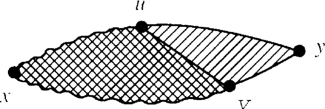
Figure 4: The amplitude (Green’s function) for transition of a glueball into a meson. Symbolic notations are the same as in Figs.1 and 3.

We come now to the amplitude of Fig.4, which gives the amplitude for glueball-meson mixing. Analysis similar to the previous one yields for this amplitude the following ratio:

$$\lambda_{n}^{GM}=\frac{\tilde{V}_{Mn}}{\sqrt{2\mu_{g}(G)}}\frac{V_{nM}}{\sqrt{2\mu_{g}(H)}}\frac{1}{|M_{G}-M_{H}^{(n)}||M_{H}^{(n)}-M_{m}|}=\lambda_{n}^{GH}\lambda_{n}^{HM}.$$ (71)

Insertion of our results (64)–(65) leads to the following order of magnitude estimate

$$\lambda_{n}^{GM}\approx N_{c}\frac{g^{2}(0.08~{}{\rm GeV})^{2}}{(\Delta M)^{2}}.$$ (72)

For $\Delta M\sim 1$ GeV one obtains $\lambda_{n}^{GM}\sim 1/16$, and the probability of admixture of the glueball to a meson $P_{GM}=|\lambda_{n}^{GM}|^{2}$ is less than a percent. This should be compared to the probability of the hybrid in the same meson

$$P_{HM}=|\lambda_{n}^{HM}|^{2}=N_{c}g^{2}\left(\frac{0.08~{}{\rm GeV}}{\Delta M}\right)^{2}\approx\lambda^{GM}_{n}\sim 5-10\%.$$ (73)

All these estimates hold for unsuppressed glueball-hybrid-meson transitions, when spin-flip amplitudes do not enter, otherwise one may expect additional one order-of-magnitude suppression of probabilities.

6 Discussion and conclusions

In Sections 4 and 5 we have obtained reduced matrix elements for meson-hybrid, hybrid-glueball, and meson-glueball transitions. The full matrix elements involve expressions of the following type (see (46) and (68)):

$$K^{MH}_{J}\equiv\int(\Phi^{(M)}_{J})^{+}_{\alpha\beta}\gamma_{\mu}\Phi^{(H)}_{J,\mu}d\tau_{3},$$ (74)

where $\Phi^{(H)}_{J,\mu}$ contains all components of the hybrid wave function.

Since the Hamiltonian (10) and the eibein technic (11) separate only positive values of $\mu_{q},\mu_{\bar{q}}$, and $\mu_{g}$, the wave functions $\Phi^{(M)}_{J}$ and $\Phi^{(H)}_{J}$ refer to those positive values and we disregard the negative energy components (negative $\mu$-components).

Moreover, spin interactions in mesons, hybrids, and glueballs are treated perturbatively in our formalism, and comparison to lattice data for the same input shows that both approximations of positive $\mu_{i}$ and perturbative spin splittings are rather good for the cases considered – see [1] for Tables with comparison. These approximations are not good for pion and kaon, where both spin and negative energy states play an important role, but we shall not consider these mesons, or hybrids with similar properties.

Therefore our parameters (50) and (69) refer only to such states which are well described by the Hamiltonian (10) with condition (11). In this case the matrix element of $\gamma_{\mu}$ is simplified since the $\mu$ dependence in the hybrid decouples from the spin (Lorentz) indices and the simplifications made after (50) are valid, when one neglects possible Clebsch–Gordon coefficients, which are of the order of unity.

In this way one obtains an estimate for the “superallowed” transitions meson-hybrid-glueball, not involving spi-flip or negative-sate components.

A comparison with the results of [5], [6] shows a good agreement within a factor of two, which tells that the missing in our case factors are of the order of unity. However, in [5],[6] as well as in our case only wave functions were considered without negative energy components (negative $\rho$-spins).

To have more comparisons, one may look at the lattice calculation of MME, which have been done extensively for the glueball $0^{++}$- scalar meson case [25, 26].

The authors [26] arrive at the following result of careful lattice studies:

$$|f_{0}(1710)>=0.859|g>+0.302|s\bar{s}>+0.413|n\bar{n}>,$$

$$|f_{0}(1500)>=-0.128|g>+0.908|s\bar{s}>-0.399|n\bar{n}>,$$

$$|f_{0}(1390)>=-0.495|g>+0.290|s\bar{s}>+0.819|n\bar{n}>.$$ (75)

¿From (75) it is clear that a strong mixing occurs between states in the region 1.4–1.7 GeV. However our results for MME between glueball and meson states always implied an appearance of a hybrid state as an intermediate state between glueball and meson. From (71) it is clear that the strong glueball-meson mixing is possible only if the intermediate hybrid has the mass in the same interval 1.4–1.7 GeV introducing in (72) $\Delta M\sim 0.2-0.3$ GeV, one obtains $\lambda_{n}^{GM}\approx 1,$ as in the lattice calculations [26] for the $0^{++}$ states.

Hence one could look for the $0^{++}$ hybrid state in the discussed mass range. Indeed, analytic calculations of lowest hybrid states in [27] confirm the possibility of the $0^{++}$ state around 1.7-1.8 GeV. this problem clearly calls for further theoretical and experimental investigation.

The author is grateful to K.A.Ter-Martirosyan for many stimulating discussions, suggestions and criticism of the first drafts of the paper. This work was partially supported by the RFFI grants 00-02-17836 and 00-15-96786.

Appendix
Meson wave-functions with definite $J^{P}$

In (21) the wave function of the meson was given in the so-called $4\times 4$ representation, where the total angular momentum $J$ and parity $P$ were not specified.

In this Appendix some relations and notations are given for meson wave functions with given $J^{P}$, based on last reference [23].

The states of the quark may be classified according to the so-called $\rho$-spin and usual spin states, where $\rho$-spin states, $\rho=\pm 1$, can be taken as eigenvalues of each of $\gamma_{0}^{(i)}~{}(i=1,2$ refer to quark 1 and quark 2, which may be an antiquark), or as eigenvalues of $\Lambda^{\pm}$, where

$$\Lambda^{\rho}(\mbox{\boldmath${\rm p}$})=\frac{\rho(\mbox{\boldmath${\rm\gamma}$}\mbox{\boldmath${\rm p}$}+m)+\gamma_{0}\sqrt{\mbox{\boldmath${\rm p}$}^{2}+m^{2}}}{2\omega}.$$ (A.1)

In both cases one can create four $\rho$-spin eigenstates (e.g., as eigenstates of $\gamma_{0}^{(1)}\gamma_{0}^{(2)}$):

$$s=\frac{|++>-|-->}{\sqrt{2}},~{}~{}a=\frac{|++>+|-->}{\sqrt{2}},$$

$$e=\frac{|+->+|-+>}{\sqrt{2}},~{}~{}O=\frac{|+->-|-+>}{\sqrt{2}}.$$ (A.2)

Using [22] one can form 8 states of unnatural parity for $qq,P=(-)^{J+1}$

$$B=\{~{}^{1}J^{s}_{J},~{}^{1}J^{a}_{J},~{}^{3}J^{s}_{J},~{}^{3}J^{a}_{J},~{}^{3}(J-1)^{e}_{J},~{}^{3}(J-1)^{0}_{J},~{}^{3}(J+1)^{e}_{J},~{}^{3}(J+1)^{0}_{J}\},$$ (A.3)

and 8 states of natural parity $P=(-)^{J}$:

$$B^{*}=\{~{}^{1}J^{e}_{J},~{}^{1}J^{0}_{J},~{}^{3}J^{e}_{J},~{}^{3}J^{0}_{J},~{}^{3}(J-1)^{s}_{J},~{}^{3}(J-1)^{a}_{J},~{}^{3}(J+1)^{s}_{J},~{}^{3}(J+1)^{a}_{J}\}.$$ (A.4)

Dynamical equations for mesons connect all components belonging to the same $J^{P}$.

The 16, component wave function (21), $f^{G_{1},G_{2}}_{\alpha_{1}\alpha_{2}}$, can be decomposed into $4\times 4$ $q\bar{q}$ basis, introduced in the last reference [22], as it is shown in the Table below.

Table 1: 16-component vector $qq$-basis states and corresponding $4\times 4$ matrix $q\bar{q}$-basis states. (The angular dependence of the wave functions of the $q\bar{q}$-triplet states must determine to which $qq$-triplet state they correspond. For a correct normalization, all matrix states should be multiplied by 1/2; furthermore, matrix states proportional to $p$ or $p$ need an extra factor $1/M$ and $1|p|$, respectively. The correspondence is only valid in the c.m.s. and $p_{0}=0$ is assumed.) Here $P$ and $p$ refer to the total and relative momentum of $q\bar{q}$ in the meson respectively.

$qq$-State	$q\bar{q}$-State
$~{}^{1}J^{s}_{J}$	$-\gamma_{5}\not{P}$
$~{}^{1}J^{a}_{J}$	$-\gamma_{5}$
$~{}^{1}J^{e}_{J}$	-1
$~{}^{1}J^{0}_{J}$	$\not{P}$
$~{}^{3}J^{s}_{J},~{}^{3}(J-1)^{s}_{J},~{}^{3}(J+1)^{s}_{J}$	$-\not p$
$~{}^{3}J^{a}_{J},~{}^{3}(J-1)^{a}_{J},~{}^{3}(J+1)^{a}_{J}$	$i\sigma_{\mu\nu}P^{\mu}p^{\nu}$
$~{}^{3}J^{e}_{J},~{}^{3}(J-1)^{e}_{J},~{}^{3}(J+1)^{e}_{J}$	$-\gamma_{5}i\sigma_{\mu\nu}P^{\mu}p^{\nu}$
$~{}^{3}J^{0}_{J},~{}^{3}(J-1)^{0}_{J},~{}^{3}(J+1)^{0}_{J}$	$\gamma_{5}\not p$

A similar expansion can be derived for the hybrid states, which include in general $16\times 3$ components. In the estimates of the present paper it is assumed that the positive energy (positive $\rho$-spin) component gives the dominant contribution to the mixing matrix element, and that spin interaction can be treated perturbatively. Then the estimates (50), (69) are modified due to kinematical coefficients (like those in the Table) by factors of the order of unity.

References

[1]
For a review and refs. see:
Yu.A.Simonov, QCD and Topics in Hadron Physics, Lectures at the
XVII International School of Physics, Lisbon, 29 September -4
October, hep-ph/9911237 (to appear in Proceedings.
[18]
V.L.Morgunov, A.Nefediev and Yu.A.Simonov,
Phys. Lett. B 459, 653 (1999).
[19]
Yu.A.Simonov, Nucl. Phys. B (in press), hep-ph/0003114.
[20]
Yu.A.Simonov, Phys. Lett. B 226, 151 (1989).
[21]
E.E.Salpeter, Phys. Rev. 87, 328 (1952).
[22] J.L.Gammel, M.T.Menzel and W.R.Wortman, Phys.
Rev. D
3, 2175 (1971); J.J.Kubis, Phys. Rev. D 6, 547 (1972); C.H.Llewellyn Smith, Ann. Phys. 53, 521 (1969)
[23]
P.C.Tiemeijer, and J.A.Tjon, Phys. Lett. B 277, 38 (1992), Phys.
Rev. C 48, 896 (1993); ibid. 49, 44 (1994); P.C.Tiemeijer, PHD Thesis, Utrecht University, 1993.
[24]
A.M.Badalian and D.I.Kitoroage, Yad. Fiz. 47, 1343
(1988); B.O.Kerbikov, M.I.Polikarpov and L.V.Shevchenko, Nucl. Phys. B
331, 19 (1990); J.-M.Richard et al., Phys. Lett. B
95, 299 (1980); B.O.Kerbikov and Yu.A.Simonov, Phys. Rev. D, hep-ph/0001243.
[25]
C.Amsler, F.Close, Phys. Lett. B 353, 385 (1995).
[26] W.Lee, D.Weingarten, Phys. Rev. D 61, 014015
(2000).