Alberta Thy 15-01 SLAC-PUB-9013 hep-ph/0110028 Threshold expansion for heavy-light systems
and flavor off-diagonal current-current correlators

Abstract

An expansion scheme is developed for Feynman diagrams describing the production of one massive and one massless particle near the threshold. As an example application, we compute the correlators of heavy-light quark currents, $\bar{b}\gamma_{\mu}u$, $\bar{b}\gamma_{5}u$, through ${\cal O}(\alpha_{s}^{2})$.

Processes mediated by $W$-bosons often involve production or annihilation of two fermions with very different masses. Examples of present interest include the $B$-meson decay constant $f_{B}$ and the single top-quark production. The basic ingredient in the analysis of such processes are correlators of heavy-light currents. For example, $f_{B}$ can be determined by relating such correlators to the measured spectrum of $B$ mesons, with help of the QCD sum rules Khodjamirian (2001).

In another important application one can use such correlators, computed perturbatively in the continuum, as an input for lattice calculations, in particular for the matching of the lattice and continuum currents. The perturbative production cross section computed close to the threshold (related to the imaginary part of the current correlators) is a convenient physical observable to perform the matching lep .

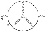
Figure 1: Examples of diagrams contributing to the current correlators at ${\cal O}\left(\alpha_{s}^{2}\right)$.

Even if the light fermion mass is neglected, a correlator still involves two mass scales (see Fig. 1), the invariant mass of the pair $\sqrt{q^{2}}$ and the mass of the heavy fermion $m$, which hampers the evaluation of the higher-order quantum effects. It is helpful to develop a computational scheme which allows to expand the Feynman diagrams around the threshold, $q^{2}=m^{2}$. In the past, various expansion schemes were constructed for other kinematical situations Chetyrkin (1991); Tkachev (1994); Smirnov (1995, 1997); Czarnecki and Smirnov (1997); Beneke and Smirnov (1998); Czarnecki and Melnikov (2001). They facilitated many studies of higher-order radiative corrections to a variety of processes of experimental importance, such as the $Z$-boson decays, heavy quark production and decays, electromagnetic properties of particles, etc. In the present paper we present an expansion scheme for the case depicted in Fig. 1, for $q^{2}\simeq m^{2}$, and apply it to compute ${\cal O}\left(\alpha_{s}^{2}\right)$ corrections to the imaginary part of the heavy-light correlators of (axial)vector as well as (pseudo)scalar currents. The real part can be obtained, if need arises, along the same lines.

Recently, numerical values of those corrections were estimated Chetyrkin and Steinhauser (2001a, b) using Padé approximants to describe the correlator as a function of $q^{2}$. The approximants were obtained from several terms in the expansion of the correlator for large ($q^{2}\gg m^{2}$) and small ($q^{2}\ll m^{2}$) values of the total energy. This approach is accurate for $q^{2}$ sufficiently far from the production threshold $q^{2}=m^{2}$. However, for practical applications related to heavy quark physics, one needs the correlators quite close to the threshold where, for kinematic reasons, their imaginary part vanishes as $(q^{2}-m^{2})^{2}$. Because of this suppression, ${\cal O}\left(\alpha_{s}^{2}\right)$ terms obtained from the Padé approximants are rather uncertain near the threshold, with an error estimated to be about $30\%$ Chetyrkin and Steinhauser (2001b).

The approach presented in this Letter enables an analytic calculation of those terms. We introduce the parameter $\delta=1-m^{2}/q^{2}$ which is small in the kinematic region close to threshold. We will show that an expansion in $\delta$ can be constructed applying the reasoning familiar from HQET directly to the Feynman diagrams. The only new ingredient necessary for a calculation of the ${\cal O}(\alpha_{s}^{2})$ corrections to the correlators are certain three-loop HQET diagrams whose calculation we will describe.

We consider the following correlator,

$$\left(-q^{2}g_{\mu\nu}+q_{\mu}q_{\nu}\right)\Pi^{v}(q^{2})+q_{\mu}q_{\nu}\Pi_{L}^{v}(q^{2})$$ (1)

$$=i\int{\rm d}xe^{iqx}\langle 0|Tj_{\mu}^{v}(x)j_{\nu}^{v}(0)|0\rangle,$$

with $j_{\mu}^{v}=\bar{\psi}_{1}\gamma_{\mu}\psi_{2}$ and $\psi_{1,2}$ denoting the Dirac spinors for the massless and massive quarks, respectively. This correlator is an analytic function of $q^{2}$ with a cut starting at $q^{2}=m^{2}$, corresponding to $\delta=0$. Since $\delta$ is proportional to the phase space available for the production of heavy and light quarks, for small $\delta$ the heavy quark is non-relativistic and always close to its mass shell. On the contrary, the massless quark is always ultrarelativistic, but its energy is small if $\delta$ is small. The HQET is designed to study exactly this kind of situation and the calculation of the relevant Feynman diagrams can be simplified if one follows its pattern.

We have to consider two different scales of the momentum $k$ flowing along a given line in a Feynman diagram: hard $k\sim m$ or soft $k\sim m\delta$. Consider the heavy quark propagator $\sim 1/(k^{2}+2qk+q^{2}\delta)$. If $k$ is hard, the propagator can be expanded in a Taylor series in $\delta$ yielding the on-shell heavy quark propagator $\sim 1/(k^{2}+2qk)$. On the other hand, if $k$ is soft, the propagator can be expanded in $k^{2}$ resulting in the static heavy quark propagator $\sim 1/(2qk+q^{2}\delta)$, familiar from HQET.

For each diagram, one has to consider all possible momentum routings and find all contributing subgraphs. Among them, there are two which can be easily described. First there is the situation when all lines are soft so that all heavy quark propagators become static and the diagram becomes what is usually referred to as a HQET matrix element. In our case, these subgraphs require three-loop calculations in HQET and we will explain below how we solve this problem.

The second type of subgraphs arises in the situation when all momenta are hard. In this case all heavy quark propagators are Taylor expanded in $\delta$; the resulting Feynman diagrams are of the on-shell three-loop propagator type, studied in Laporta and Remiddi (1993); Melnikov and van Ritbergen (2000), and their evaluation is possible. However, since these contributions are polynomials in $\delta$, they do not contribute to the imaginary part of the correlator and we do not consider them here.

In between the two extreme cases discussed above, there are situations where, in a given diagram, some of the lines are soft and some are hard. Using the HQET language, these correspond to the HQET matrix elements with insertions of higher dimensional operators of the HQET Lagrangian or to the HQET matrix elements computed with leading order operators (HQET currents) corrected for the higher order Wilson coefficients. Since the Wilson coefficients are computed at the hard scale, such contributions factorize into products of simple subgraphs and can be easily computed.

Therefore, the main challenge are the three-loop HQET diagrams. There are two ways to compute them and we have taken both to have a cross check. Recently, the three-loop HQET diagrams have been analyzed in Grozin (2000, 2001) and a computer algebra program has been published, capable of computing all three-loop HQET propagator type diagrams. We have used that software to calculate the required HQET matrix elements. For the purpose of the cross check, we have written (in FORM Vermaseren ), in a completely independent way, a similar program solving the three-loop recurrence relations for HQET propagator-type integrals, restricting ourselves to topologies needed for the current calculation.

In both approaches, every Feynman diagram is expressed in terms of a few master integrals. The majority of them is known Grozin (2000, 2001); Beneke and Braun (1994). However, one of the master integrals has not been evaluated to sufficient accuracy in the existing literature and we have to compute it. It turns out that one can use a trick to this end. The Euclidean integral we need is ($p^{2}=-1$, $d=4-2\epsilon$):

$$I = \int\frac{{\rm d}^{d}k_{1}{\rm d}^{d}k_{2}{\rm d}^{d}k_{3}}{k_{1}^{2}k_{3}^{2}(k_{1}-k_{2})^{2}(k_{3}-k_{2})^{2}}$$ (2)

$$\times\frac{1}{(2pk_{1}+1)(2pk_{2}+1)(2pk_{3}+1)}.$$

To compute it, consider a similar integral,

$$I_{1} = \int\frac{{\rm d}^{d}k_{1}{\rm d}^{d}k_{2}{\rm d}^{d}k_{3}}{k_{1}^{2}k_{2}^{2}k_{3}^{2}(k_{1}-k_{2})^{2}(k_{3}-k_{2})^{2}}$$ (3)

$$\times\frac{1}{(2pk_{1}+1)(2pk_{2}+1)(2pk_{3}+1)},$$

related to $I$ by integration-by-parts Chetyrkin and Tkachev (1981) identities. We perform a transformation $|k_{i}|\to 1/|k_{i}|$ for $i=1,2,3$ in Eq. (3). The integral $I_{1}$ transforms to

$$I_{1} = \int\frac{{\rm d}^{d}k_{1}{\rm d}^{d}k_{2}{\rm d}^{d}k_{3}}{k_{1}^{2d-6}k_{2}^{2d-8}k_{3}^{2d-6}(k_{1}-k_{2})^{2}(k_{3}-k_{2})^{2}}$$ (4)

$$\times\frac{1}{(2pk_{1}+k_{1}^{2})(2pk_{2}+k_{2}^{2})(2pk_{3}+k_{3}^{2})}.$$

In the next step we notice that $I_{1}$ is finite in four dimensions, so that the limit $d\to 4$ can be taken; after that $I_{1}$ becomes equal to one of the on-shell three-loop master integrals computed in Melnikov and van Ritbergen (2000). We therefore find:

$$I_{1}=C(\epsilon)\left[2\pi^{2}\zeta_{3}-5\zeta_{5}\right]+{\cal O}(\epsilon),$$ (5)

with $C(\epsilon)=[\pi^{2-\epsilon}\Gamma(1+\epsilon)]^{3}$. We now use recurrence relations to obtain $I$ from $I_{1}$ and derive:

$$I = C(\epsilon)\left[-\frac{\pi^{2}}{18\epsilon^{2}}+\frac{1}{\epsilon}\left(-\frac{4\pi^{2}}{9}+\frac{1}{3}\zeta_{3}\right)\right.$$ (6)

$$\left.+\left(\frac{8}{3}\zeta_{3}-\frac{26\pi^{2}}{9}-\frac{17\pi^{4}}{540}\right)+\epsilon\left(-\frac{4\pi^{2}}{9}\zeta_{3}\right.\right.$$

$$\left.\left.+\frac{52}{3}\zeta_{3}-\frac{160\pi^{2}}{9}-\frac{34\pi^{4}}{135}-\frac{83}{3}\zeta_{5}\right)+{\cal O}(\epsilon^{2})\right].$$

With this integral at hand, all the three-loop HQET master integrals are available to sufficiently high power in their expansion in $\epsilon$ and we can proceed with the computation of the correlators.

Figure 2: $N_{c}\delta^{2}\Delta^{v}_{\rm A,NA,L,H}$ plotted as a function of $v=\delta/(2-\delta)$.

We introduce the dimensionless quantity

$$R^{v}(q^{2})\equiv{\Gamma(W^{\star}\to b\bar{u})\over|V_{bu}|^{2}\Gamma(W^{\star}\to e\bar{\nu})}=12\pi{\rm Im}\left[\Pi^{v}(q^{2}+i\delta)\right],$$ (7)

and expand it in a series in the strong coupling constant (we use the $\overline{\rm MS}$ scheme and denote $a\equiv\alpha_{s}(M)/\pi$)

$$R^{v}\simeq N_{c}\left(R_{0}^{v}+C_{F}aR_{1}^{v}+C_{F}a^{2}R_{2}^{v}\right),$$ (8)

We find (an exact formula for $R^{(1),v}\equiv N_{c}R_{1}^{v}$ can be found in Chetyrkin and Steinhauser (2001b), eq. (9)):

$$R_{0}^{v} = \frac{\delta^{2}(3-\delta)}{2}$$

$$R_{1}^{v} = \frac{3\delta^{2}}{4}\left[\left(\frac{9}{2}-3\ln\delta+\frac{2}{3}\pi^{2}\right)\right.$$

$$\left.+\delta\left(\frac{-139}{18}+\frac{11}{3}\ln\delta-\frac{2}{9}\pi^{2}\right)\right]+{\cal O}(\delta^{4}),$$

$$R_{2}^{v} = \delta^{2}\left(C_{F}\Delta_{A}^{v}+C_{A}\Delta_{NA}^{v}+T_{R}N_{L}\Delta_{L}^{v}+T_{R}\Delta_{H}^{v}\right).$$ (9)

For the individual color structures we obtain:

$$\Delta_{A}^{v}=\frac{523}{64}-\frac{39}{8}\zeta_{3}+\frac{7\pi^{2}}{4}\ln 2+\frac{5\pi^{2}}{12}+\frac{\pi^{4}}{60}$$

$$-\left(\frac{5\pi^{2}}{4}+\frac{147}{32}\right)L_{\delta}+\frac{27}{16}L_{\delta}^{2}$$

$$+\delta\left[-\frac{10079}{576}+\frac{39}{8}\zeta_{3}-\frac{19\pi^{2}}{12}\ln 2-\frac{575\pi^{2}}{432}-\frac{\pi^{4}}{180}\right.$$

$$\left.+\left(\frac{53\pi^{2}}{36}+\frac{1339}{96}\right)L_{\delta}-\frac{57}{16}L_{\delta}^{2}\right]+\delta^{2}\left[\frac{1819}{144}\right.$$

$$\left.-\frac{5\pi^{2}}{24}\ln 2+\frac{421\pi^{2}}{1728}+\left(\frac{\pi^{2}}{72}-\frac{395}{48}\right)L_{\delta}+\frac{17}{16}L_{\delta}^{2}\right],$$

$$\Delta_{NA}^{v}=\frac{1103}{64}-\frac{129}{16}\zeta_{3}-\frac{7\pi^{2}}{8}\ln 2+\frac{427}{288}\pi^{2}-\frac{\pi^{4}}{60}$$

$$-\left(\frac{19\pi^{2}}{24}+\frac{423}{32}\right)L_{\delta}+\frac{33}{16}L_{\delta}^{2}$$

$$+\delta\left[-\frac{42655}{1728}+\frac{33}{16}\zeta_{3}+\frac{19\pi^{2}}{24}\ln 2-\frac{\pi^{2}}{9}+\frac{\pi^{4}}{180}\right.$$

$$\left.-\left(\frac{\pi^{2}}{24}-\frac{4685}{288}\right)L_{\delta}-\frac{115}{48}L_{\delta}^{2}\right]+\delta^{2}\left[\frac{7931}{3456}-\frac{\zeta_{3}}{16}\right.$$

$$\left.+\frac{5}{48}\pi^{2}\ln 2-\frac{115}{1152}\pi^{2}-\left(\frac{\pi^{2}}{48}-\frac{305}{576}\right)L_{\delta}-\frac{17}{48}L_{\delta}^{2}\right],$$

$$\Delta_{L}^{v}=-\frac{117}{16}+3\zeta_{3}-\frac{7\pi^{2}}{36}+\left(\frac{\pi^{2}}{3}+\frac{39}{8}\right)L_{\delta}-\frac{3}{4}L_{\delta}^{2}$$

$$+\delta\left[\frac{3671}{432}-\zeta_{3}-\frac{5\pi^{2}}{108}-\left(\frac{\pi^{2}}{9}+\frac{397}{72}\right)L_{\delta}+\frac{11}{12}L_{\delta}^{2}\right]$$

$$+\delta^{2}\left(-\frac{721}{864}+\frac{1}{18}L_{\delta}+\frac{1}{12}L_{\delta}^{2}\right),$$

$$\Delta_{H}^{v}={133\over 32}-{5\pi^{2}\over 12}+\delta\left(-{1997\over 864}+{\pi^{2}\over 4}\right)$$ (10)

$$+\delta^{2}\left({2473\over 10800}-{1\over 20}L_{\delta}-{\pi^{2}\over 72}\right).$$

We denoted $L_{\delta}=\ln\delta$ and the zeta function $\zeta_{3}\simeq 1.202$. We do not display higher order terms in the expansion in $\delta$, but they can be easily obtained as well.

For completeness, we also give the results for ${\cal O}(\alpha_{s}^{2})$ correction to the correlator of two scalar currents. Let us define

$$q^{2}\Pi^{s}(q^{2})=i\int{\rm d}xe^{iqx}\langle 0|Tj^{s}(x)j^{s}(0)|0\rangle,$$ (11)

where $j_{s}=Z_{\rm m}\bar{\psi}_{1}\psi_{2}$ and, again, $\psi_{1,2}$ denote the Dirac spinors for the massless and massive quarks and $Z_{\rm m}$ is the on-shell mass renormalization constant for the massive quark. We define

$$R^{s}(q^{2}) = 8\pi{\rm Im}\left[\Pi^{s}(q^{2}+i\delta)\right],$$ (12)

$$\simeq N_{c}\left(R_{0}^{s}+C_{F}aR_{1}^{s}+C_{F}a^{2}R_{2}^{s}\right).$$

We then find (for an exact formula for $R_{1}^{s}$ see Chetyrkin and Steinhauser (2001b))

$$R_{0}^{s} = \delta^{2},$$

$$R_{1}^{s} = \delta^{2}\left[\left(\frac{13}{4}-\frac{3}{2}L_{\delta}+\frac{1}{3}\pi^{2}\right)-3\delta\right]+{\cal O}(\delta^{4}),$$

$$R_{2}^{s} = \delta^{2}\left(C_{F}\Delta_{A}^{s}+C_{A}\Delta_{NA}^{s}+T_{R}N_{L}\Delta_{L}^{s}+T_{R}\Delta_{H}^{s}\right).$$

For the individual color structures we obtain:

$$\Delta_{A}^{s}={229\over 32}+{\pi^{2}\over 2}\ln 2+{3\over 2}\pi^{2}+{\pi^{4}\over 90}-{9\over 4}\zeta_{3}$$

$$-\left({5\over 6}\pi^{2}+{73\over 16}\right)L_{\delta}+{9\over 8}L_{\delta}^{2}$$

$$+\delta\left[-{493\over 48}-{115\over 72}\pi^{2}-{3\over 2}\zeta_{3}+\left(4-{\pi^{2}\over 3}\right)L_{\delta}\right]$$

$$+\delta^{2}\left[-{4325\over 864}-{\pi^{2}\over 4}\ln 2-{671\over 864}\pi^{2}+{1\over 2}\zeta_{3}\right.$$

$$\left.\qquad+\left({245\over 36}+{7\over 36}\pi^{2}\right)L_{\delta}-{29\over 24}L_{\delta}^{2}\right]$$

$$\Delta_{NA}^{s}={4361\over 288}-{\pi^{2}\over 4}\ln 2+{283\over 432}\pi^{2}-{\pi^{4}\over 90}-{47\over 8}\zeta_{3}$$

$$\qquad-\left({19\over 36}\pi^{2}+{141\over 16}\right)L_{\delta}+{11\over 8}L_{\delta}^{2}$$

$$+\delta\left[-{949\over 72}-{31\over 432}\pi^{2}-{\zeta_{3}\over 4}+\left({11\over 3}-{\pi^{2}\over 18}\right)L_{\delta}-{1\over 4}L_{\delta}^{2}\right]$$

$$+\delta^{2}\left[-{4651\over 864}+{\pi^{2}\over 8}\ln 2+{179\over 1728}\pi^{2}-{1\over 4}\zeta_{3}\right.$$

$$\left.\qquad+\left({283\over 96}-{7\over 72}\pi^{2}\right)L_{\delta}-{5\over 12}L_{\delta}^{2}\right]$$

$$\Delta_{L}^{s}=-{427\over 72}-{7\over 54}\pi^{2}+2\zeta_{3}+\left({2\over 9}\pi^{2}+{13\over 4}\right)L_{\delta}-{1\over 2}L_{\delta}^{2}$$

$$+\delta\left({163\over 36}+{2\over 9}\pi^{2}-{4\over 3}L_{\delta}\right)+\delta^{2}\left({623\over 432}-{19\over 18}L_{\delta}+{1\over 6}L_{\delta}^{2}\right)$$

$$\Delta_{H}^{s}={727\over 144}-{\pi^{2}\over 2}+{2\over 9}\delta+\delta^{2}\left({1\over 36}\pi^{2}-{67\over 2700}-{1\over 30}L_{\delta}\right)$$ .

The results for the pseudo-scalar and axial-vector currents are the same as for the scalar and vector currents because the presence of massless fermion line permits one to cancel the Dirac $\gamma_{5}$ matrices.

It is interesting to compare our results with the numbers obtained in Chetyrkin and Steinhauser (2001b). We have plotted our results for the independent color structures as functions of the velocity $v=\delta/(2-\delta)$ using our results for $R_{2}^{v}$, including terms ${\cal O}\left(\delta^{5}\right)$ which we do not display in (10). Comparing these results with Fig. 4 of Chetyrkin and Steinhauser (2001b), we find very good agreement for $v\leq 0.6$ KGNumbers ; for larger values of $v$ our truncated series is not accurate (as can be expected from the very nature of expansion) and more terms in the expansion are needed. We have also verified the relations between the scalar and vector correlators given in eqs. (32-33) in Chetyrkin and Steinhauser (2001b).

In Chetyrkin and Steinhauser (2001b), the values of the ${\cal O}(\delta^{2}\ln^{0}\delta)$ terms were estimated by fitting numerical solutions. Our formulas provide analytic results for these coefficients. In the notation of eq. (45) of Chetyrkin and Steinhauser (2001b), we find

$$\tilde{c}_{FF} = \frac{1173}{128}+\frac{103\,{\pi}^{2}}{48}+\frac{{\pi}^{4}}{90}-\left(\frac{97}{16}+\frac{5\,\pi^{2}}{6}\right)\ln 2$$

$$+\frac{9}{8}\ln^{2}2-\frac{\zeta_{3}}{2}\simeq 21.46,$$

$$\tilde{c}_{FA} = \frac{20057}{1152}+\frac{119\,{\pi}^{2}}{216}-\frac{{\pi}^{4}}{90}-\left(\frac{141}{16}+\frac{19\,\pi^{2}}{36}\right)\ln 2$$

$$+\frac{11}{8}\ln^{2}2-\frac{13\,\zeta_{3}}{2}\simeq 4.894,$$

$$\tilde{c}_{FL} = -\frac{1849}{288}-\frac{23\,{\pi}^{2}}{108}+\left(\frac{13}{4}+\frac{2\,{\pi}^{2}}{9}\right)\ln 2$$ (15)

$$-\frac{{\ln^{2}2}}{2}+2\,\zeta_{3}\simeq-2.585.$$

These results agree well with the estimates of Chetyrkin and Steinhauser (2001b) for the the abelian $\tilde{c}_{FF}=21(6)$ and the light quark $\tilde{c}_{FL}=-2.3(7)$ contributions. The non-abelian part found in Chetyrkin and Steinhauser (2001b), $\tilde{c}_{FA}=1.2(4)$, differs by about 9 sigma from our result, 4.894. Since the production threshold is the most difficult place for the Padé approximants it is very likely KG that the accuracy of this particular result was overestimated in Chetyrkin and Steinhauser (2001b).

The expansion around the heavy-light threshold presented here extends the class of Feynman diagrams which can be evaluated analytically. Our approach can be summarized as applying the HQET directly to Feynman diagrams. As an example application, we computed the imaginary part of flavor off-diagonal current correlators to ${\cal O}(\alpha_{s}^{2})$ useful as an input for both $f_{B}$ determination from QCD sum rules and also for matching of the lattice and continuum currents. Similar techniques can be used to study second order QCD corrections to differential distributions in heavy to light semileptonic decays. Work on this is in progress.

We are grateful to G. P. Lepage for a conversation which stimulated this study. This research was supported in part by the Natural Sciences and Engineering Research Council of Canada and by the DOE under grant number DE-AC03-76SF00515.

References

• Khodjamirian (2001) For a recent review and references to original papers see A. Khodjamirian (2001), eprint hep-ph/0108205.
• (2) We are indebted to G. P. Lepage for a discussion of this point.
• Chetyrkin (1991) K. G. Chetyrkin (1991), preprint MPI-Ph/PTh 13/91.
• Tkachev (1994) F. V. Tkachev, Sov. J. Part. Nucl. 25, 649 (1994), eprint hep-ph/9701272.
• Smirnov (1995) V. A. Smirnov, Mod. Phys. Lett. A10, 1485 (1995), eprint hep-th/9412063.
• Smirnov (1997) V. A. Smirnov, Phys. Lett. B404, 101 (1997), eprint hep-ph/9703357.
• Czarnecki and Smirnov (1997) A. Czarnecki and V. Smirnov, Phys. Lett. B394, 211 (1997), eprint hep-ph/9608407.
• Czarnecki and Melnikov (2001) A. Czarnecki and K. Melnikov, Phys. Rev. Lett. 87, 013001 (2001), eprint hep-ph/0012053.
• Beneke and Smirnov (1998) M. Beneke and V. A. Smirnov, Nucl. Phys. B522, 321 (1998), eprint hep-ph/9711391.
• Chetyrkin and Steinhauser (2001a) K. G. Chetyrkin and M. Steinhauser, Phys. Lett. B502, 104 (2001a), eprint hep-ph/0012002.
• Chetyrkin and Steinhauser (2001b) K. G. Chetyrkin and M. Steinhauser, Eur. Phys. J. C21, 319 (2001b), eprint hep-ph/0108017.
• Laporta and Remiddi (1993) S. Laporta and E. Remiddi, Phys. Lett. B301, 440 (1993).
• Melnikov and van Ritbergen (2000) K. Melnikov and T. van Ritbergen, Nucl. Phys. B591, 515 (2000), eprint hep-ph/0005131.
• Grozin (2000) A. G. Grozin, JHEP 03, 013 (2000), eprint hep-ph/0002266.
• Grozin (2001) A. G. Grozin (2001), eprint hep-ph/0107248.
• (16) J. A. M. Vermaseren, math-ph/0010025.
• Beneke and Braun (1994) M. Beneke and V. M. Braun, Nucl. Phys. B426, 301 (1994), eprint hep-ph/9402364.
• Chetyrkin and Tkachev (1981) K. G. Chetyrkin and F. V. Tkachev, Nucl. Phys. B192, 159 (1981).
• (19) We are grateful to K. G. Chetyrkin for providing sample numerical values for comparisons.
• (20) K. G. Chetyrkin, private communication.