Real Time Dynamics of Symmetry Breaking

Zsolt Szép

Ph.D. Thesis

Supervisor: András Patkós

physics program

program leader: Horváth Zalán

subprogram leader: George Pócsik

Department of Atomic Physics

Eötvös Loránd University, Budapest

September 2001

Chapter 1 Introduction and motivation

In the last few years remarkable progress has been made in the investigation of the non-equilibrium behaviour of finite temperature systems, both for scalar and gauge fields. Actually, after understanding equilibrium features of these systems many of the workers in the field have eagerly blazed away at investigating non-equilibrium aspects of finite temperature Quantum Field Theories, with a special emphasis on the real time simulation of its high temperature limit. There are a few good reasons for doing this.

First of all, time dependent phenomena in hot relativistic quantum field theory play an important role in applications to cosmology, in the context of baryogenesis and inflation, and in the heavy ion collisions. Not all of these phenomena are non-perturbative (for example relaxation phenomena to equilibrium from states slightly out of equilibrium can be treated perturbatively) but as the departure from equilibrium increases non-perturbative tools are needed. Non-perturbative calculations under general circumstances are very difficult. Real time numerical simulations in the QFT would face the problem of complex weights appearing in the quantum expectation value of time dependent quantities. Fortunately a classical description can be accurate for physical quantities which are determined by low momentum modes of the theory, because these modes are highly occupied at high enough temperature. For high momentum modes, the classical treatment is incorrect, but in general the influence of these modes can be taken into account perturbatively. Initially proposed in [1] for the computation of the rate of sphaleron transitions, the numerical solution of the classical approximation proved to be eventually a powerful tool in evaluating quantities for systems developing in time.

Preheating and the possibility of Electroweak baryogenesis

An intensively investigated field is the transition from an inflationary to the radiation dominated epoch in the early Universe. In the context of chaotic inflation [2] it was realised that the initially homogeneous inflaton field can decay very rapidly into narrow bands of its own low momentum modes or into modes of other scalar fields through parametric resonance. This phenomenon goes by the name of preheating.

The large amplitudes of the parametrically amplified modes make this problem non-perturbative, but at the same time the large occupation number of these modes opens the possibility to study this problem in the classical field approximation on lattice (for example [3] and references therein). It was then realised that in addition to the standard high-temperature phase transitions that is assumed to occur in the state of thermal equilibrium [4], there exists a new class of phase transitions which may occur at the intermediate stage between the end of inflation and the establishing of thermal equilibrium [5, 6]. These new types of phase transitions are referred as to cosmological non-thermal phase transitions after preheating, and can restore symmetry on scales up to $10^{16}$ GeV, due to large amplitude non-thermal fluctuations. An important feature of the non-thermal phase transition based on preheating is that the classical non-linear dynamics of inflaton field coupled with other boson fields can induce symmetry breaking for the latter.

Symmetry breaking is a fundamental component of theoretical particle physics because through the Higgs effect it accounts for the masses of the elementary particles. These particles have got their masses during the electroweak phase transition. The importance of this phase transition is revealed by its impact on the observed baryon asymmetry in our Universe. A successful theory of baryogenesis requires beyond the existence of baryon number violating processes C and CP violating processes and departure from thermal equilibrium. These three requirements are known as Sakharov conditions. In the standard model (SM) baryon number is not conserved because of the non-perturbative processes in the gauge sector that involve the quantum anomaly. The usual scenario assumes that the universe was in thermal equilibrium before and after the electroweak phase transition, and far from it during the phase transition. In order to significantly drive the primordial plasma out of equilibrium a strongly first order phase transition is needed. This is also a condition for the sphaleron processes to stop quickly after the transition in order to prevent the washing out of the created baryon asymmetry. The order of the EW phase transition was thoroughly analysed, both perturbatively [7] and with MC simulations [8, 9] and the conclusion was, that there is an end point on the line of the first order phase transition separating the symmetric and broken phases at a Higgs mass of about $\approx$ 72 GeV. For greater Higgs mass values there is no first order PT that makes the things hopeless in view of the LEP experiments that exclude a Higgs mass below 113 GeV. So, the possibility of baryogenesis in the usual scenario is ruled out in the SM. This also means that if the EWPT occurred in thermal equilibrium then the onset of the Higgs effect was a smooth process.

In the usual scenario one can go to a minimal supersymmetric extension of the SM. The phase structure of MSSM is much more difficult to explore because of its large parameter space. According to perturbation theory and 3-dimensional lattice simulations [10] as well as 4-dimensional lattice simulation [11], there could be an EWPT in MSSM that is strong enough for baryogenesis up to a value of $\approx$ 105 GeV for the lightest Higgs mass.

Recently it was shown that the baryogenesis can take place below the EW scale in a very economical extension of the SM in which only one more scalar $SU(2)\times U(1)$-singlet field is required, to be taken the inflaton [12, 13]. The novel scenario make use of the possibilities that reside in the phenomena of preheating. The preheating precedes the establishment of thermal equilibrium. With an appropriate choice of the parameters of the inflation one can achieve that the reheating temperature remains below the EW scale, therefore no intensive sphaleron processes are allowed. There is an important baryon asymmetry production during rescattering after preheating due to the fact that the low modes that carry a large amount of the energy quickly “thermalize” at a high effective temperature (a few times the value of the EW scale) where the rate of sphaleron transitions is very effective.

Thermalization and relaxation

The approach to equilibrium of initially out-of-equilibrium states is a highly important issue in many branches of physics ranging from inflationary cosmology (the spectrum of density fluctuation in the early universe) through particle physics (the problem of baryogenesis, formation of DCC in heavy ion collisions) to statistical physics (dynamics of phase transitions, realization of Boltzmann’s conjecture that is an ensemble of isolated interacting systems eventually approaches thermal equilibrium at large times.)

In the recent field theoretical studies of thermalization and relaxation classical fields are intensively investigated [14]. The interest stems from the fact that in order to explore the reliability of truncation and expansion schemes they should be benchmarked against this exact solution. Recently, evolution of equal-time 1PI correlation functions derived from the effective time dependent action [15] were confronted with the results of the exact time evolution. By solving equations non-local in time, obtained from 2PI effective action thermalization of quantum fields was demonstrated [16]. These approximate methods can be formulated both for classical and quantum cases. In the quantum case the analogue of the classical ensemble averaging over the initial conditions is the quantum expectation value. With this correspondence the formal derivations, and hence the results, are quite similar [17].

Heavy Ion collision

Two phenomena of the QCD chiral phase transition have received much attention in the past decade due to the fact that both may be within reach of discovery by the current or forthcoming relativistic heavy-ion collision experiments: the formation of disoriented chiral condensate (DCC) and the end point (the critical point $E$) of the first order phase transition line for decreasing chemical potential $\mu$ in the $\mu-T$ QCD phase diagram.

When both areas are studied in the context of heavy-ion collision experiments a knowledge of the evolution of far from equilibrium dynamical system of strongly interacting quantum fields of bosonic and fermionic degrees of freedom is needed. During the evolution the system rapidly expands and cools creating and emitting baryons and mesons.

As investigating such systems and in particular phase transitions directly in QCD is out of question at the moment, a model that encodes relevant aspects of QCD in a faithful manner is needed.

It was argued in [18] that the O(4)-symmetric linear $\sigma$-model is representative of the physics relevant for the formation of DCC. This model is in the same static universality class as the QCD with two massless quarks, that is a good approximation to the world at temperatures and energies below $\lambda_{QCD}$. The basic idea of DCC formation is that regions of misaligned vacuum might occur. These are regions where the field $\Phi^{a}\equiv(\sigma,\vec{\pi})$ instead of taking the true ground state value $(v,0)$ is partially aligned with the $\pi$ direction. It is expected that the relaxation of the misaligned vacuum region to the true vacuum would proceed through coherent pion emission with a charge distribution violating the isospin symmetry. For energetical reasons (see Ref. [18] ) the emission of a large number of pions that produce an easily detectable signal could only be envisaged in a highly non-thermal chiral phase transition, that is when the system is far out of equilibrium. This situation is approximated with a sudden quench from high to low temperature during which the long wavelength modes of the pion fields become unstable and grow relative to the short wavelength ones.

At the critical point $E$ the phase transition is second order and belongs to the Ising universality class. The pions remain massive but the correlation length of the $\sigma$ field, that plays the role of the order parameter, diverges due to growing long wavelength fluctuations. An increase in the correlation length compared with the one corresponding to the equilibrium energy density of the QCD plasma can be observed by analysing the low transversal momentum pions in which the $\sigma$ fields decay.

At present it is not possible to construct the exact mapping between the axes of QCD phase diagrams and the axes of the Ising phase diagrams. With the new possibility of simulating the QCD phase diagram at non-zero chemical potential proposed in [19] this question may be solved in the near future.

Critical slowing down that occurs near the critical point $E$ requires long equilibration times meaning that the plasma will inevitably slow out of equilibrium if the plasma is cooled. Since the rate of cooling is faster than the rate at which the system can adapt to this change, a non-equilibrium evolution is guaranteed.

The phenomenon we are interested in both cases cited above is related to the growth of the correlation length basically produced by the long wavelength, classical modes. This is an argument favouring classical real time numerical simulations. The inclusion of quantum correction is an important question and has been implemented in mean-field approximation.

Recently the effect of dynamical behaviour of the $\sigma$ correlation length around the critical point $E$ was studied in Ref. [20]. An intuitive mapping between QCD and the Ising model was proposed identifying the magnetic field and the reduced temperature of the Ising model with the temperature of the QCD and the chemical potential, respectively. The result of the investigation, a factor of 2-3 increase in the correlation length proved to be insensitive to moderate tilt in this mapping. In Ref. [21] basically the same investigation was performed with a second order dynamics in the context of $\Phi^{4}$ theory.

The classical approximation and its problems.

It is well known that at high temperature the thermodynamics of a QFT in ($3+1$) dimensions is successfully described through dimensional reduction (DR) by an effective classical 3 dimensional theory derived for the static modes of the original theory. Its couplings are determined by the integration over the non-static modes [22, 23]. Corrections to the dimensional reduction are small when the thermal mass and external momenta are small compared to the temperature, a requirement that is satisfied when the theory is weakly coupled. Unlike the case of QFT at finite temperature where the Bose-Einstein distribution effectively introduces an UV-cutoff, the formulation of a classical field theory is meaningful only if a $\Lambda$ UV-cutoff is present, otherwise one encounters the Rayleigh-Jeans divergences. The introduction of $\Lambda$ means that the parameters of the effective theory must depend on it in such a way as to cancel the $\Lambda$-dependence of the regularized loop integrals in the effective theory.

Encouraged by the success of DR one could naively expect that the dynamics of soft modes is described by classical Hamiltonian dynamics i.e. calculation of time dependent correlation functions implies solving classical Hamiltonian equations of motion for arbitrary initial conditions, over which a Boltzmann weighted averaging with the 3 dimensional DR action is performed. This was the essence of the proposal of Grigoriev and Rubakov [1] for calculating time dependent correlation functions. The expectation above works only for scalar $\Phi^{4}$ theory and for Abelian-gauge theory in ($1+1$) dimension. In the former case it was shown that the ultraviolet divergences of the time dependent correlation functions can be absorbed by the same mass counterterms as needed in the static theory [24].

For non-Abelian gauge theory in higher spatial dimensions the dynamics of infrared fields is classical, but they are not described by classical Hamiltonian dynamics. Here the problem of UV divergences is more involved. Actually, the existence of a classical theory poses two questions: 1. what is the divergence structure of the hot real time classical Yang-Mills theory 2. if there are well-separated scales in the theory (for example in a gauge theory) what is the interplay between them. The answer to the first question is, that at one loop the linear divergences of the classical theory are related to the quantum hard thermal loops (HTL) discovered by Braaten and Pisarski. For example, the divergent part of the classical self-energy can be obtained as the classical limit of HTL self energy [25, 26, 27]. It was realised in [25] that there are UV divergences in the classical thermal Yang-Mills theory which are non-local in space and time (on the lattice they are sensitive to the lattice geometry), they do not occur in equal time correlation functions and so they cannot be absorbed by local counterterms. The second question led in the end to the serious challenge of constructing an effective theory for the low-momentum modes by incorporating as accurately as possible the effect of the quantum but perturbative high-momentum modes. This step has to be done if the classical theory exhibits strong cut-off dependence, or equivalently lattice-spacing dependence, because if this occurs it shows that the classical dynamics is sensitive to quantum modes with momenta of the order of the cutoff.

In non-Abelian gauge theory at temperatures where the weak coupling limit is valid, there is a hierarchy of three momentum scales that played an important role already in the static case [28, 29]. There is the “hard” scale $T$ of the typical momentum of a particle, there is the “soft” scale $gT$ associated with colour-electric screening and finally there is the “ultrasoft” scale $g^{2}T$ associated with colour-magnetic screening and where non-perturbative effects appear.

The first numerical simulations were done in a purely Yang-Mills classical theory with a cutoff $\Lambda$ of order $T$, but it raised the suspicion of a strong cutoff dependence of the measured quantity, the sphaleron rate. This indeed was the case as shown for example in [30].

One can incorporate the effect of the “hard” modes of order $\sim T$ on the dynamics of softer modes using a classical theory based on the HTL effective action obtained after integrating out these modes. There are difficulties with this approach due to the fact that the HTL equations of motions are non-local in space and time and a local Hamiltonian form exists only in the continuum.

The classical effective HTL theory leads to UV divergences and has to be defined with an UV-cutoff $gT\ll\Lambda\ll T$. In order to ensure the UV insensitivity, the coefficients of the effective theory (effective HTL Hamiltonian) must be calculated with an infrared cutoff $\Lambda$, so that the cutoff dependence of the parameters in the effective theory cancels against the cutoff dependence of the classical thermal loops. The problem is, that on the lattice it is very difficult to derive the expression of the $\Lambda$ (IR cutoff)-dependent piece in the HTL Hamiltonian.

In order to reduce the sensitivity to the UV scale $\Lambda$ one can go further and integrating out the soft degrees of freedom down to scale $g^{2}T\ll\Lambda\ll gT$ starting from the classical effective theory for the soft fields. This was first performed by Bödeker, who showed that the resulting theory at the scale $g^{2}T$ takes the form of a Boltzmann-Langevin equation [33]. It was demonstrated later that this equation is insensitive to the ultraviolet fluctuations [34].

Presentation of the thesis

This thesis reflects the route followed by its author towards the derivation of the dynamical equations allowing the study of the real time onset of the Higgs-effect. Since this study would involve both analytical and numerical investigations we have developed and tested both techniques in simpler models.

First, I have investigated the dynamics of the one-component scalar theory both in the linear-response approximation and then for large deviations from equilibrium.

Next, I proceeded to the real time characterisation of the Goldstone effect when a condensate breaks the O(N) symmetry of the field theory. Here again both quantum and classical systems were studied.

Finally, I have studied the corrections to the Hard Thermal Loop dynamics in the Abelian Higgs model, which reflect the presence of the scalar condensate.

I have five publications related to my thesis:

• A. Patkós, Zs. Szép, Phys. Lett. B446 (1999) 272-277

• A. Jakovác, A. Patkós, P. Petreczky, Zs. Szép, Phys. Rev. D61 (2000) 025006

• Sz. Borsányi, A. Patkós, Zs. Szép, Phys. Lett. B469 (1999) 188-192

• Sz. Borsányi, A. Patkós, A. Polonyi, Zs. Szép, Phys. Rev. D62 (2000) 085013

• Sz. Borsányi, Zs. Szép, Phys. Lett. B508 (2001) 109-116

The structure of the thesis is as follows.

In Chapter 2 I briefly review the formalism we use in the following Chapters: the Green-function approach to transport theory of quantum scalar fields developed by Danielewicz and Mrówczyński and the classical linear response theory of Jakovác and Buchmüller. I show the connection between the former method with others existing in the literature.

In Chapter 3 I present the work done within the one-component scalar $\Phi^{4}$ model. An effective theory of low frequency fluctuations of selfinteracting scalar fields is constructed in the broken symmetry phase coupled to the particles of a relativistic scalar gas via their locally variable mass. The non-local dynamics of Landau damping is investigated in a kinetic gas model approach.

Next, I present a numerical investigation of the thermalization in the broken phase of classical $\Phi^{4}$ theory in $2+1$ dimensions. The $\Phi$ field is coupled with a homogeneous external “magnetic” field that induces a transition from a metastable state to the stable ground state. The dynamics of the system is described using an effective equation of the order parameter. This description is consistent with the nucleation theory in a first order phase transition.

Chapter 4 also consists of two Sections. In the first one an effective theory of the soft modes in the broken phase of $O(N)$ symmetric $\Phi^{4}$ model is presented to linear approximation in the background when the effect of high-frequency fluctuations is taken into account at one-loop level. The damping of Higgs and Goldstone modes is studied together with large time asymptotic decay of an arbitrary initial configuration.

In the second Section the real time thermalization and relaxation phenomena are numerically studied in a $2+1$ dimensional classical $O(2)$ symmetric scalar theory. The near-equilibrium decay rate of on-shell waves and the power law governing the large time asymptotics of the off-shell relaxation is checked to agree with the analytic results based on linear response theory. The realisation of the Mermin-Wagner theorem is also studied in the final equilibrium ensemble.

Chapter 5 deals with the real time dynamics of the Higgs effect. The effective equations of motion for low-frequency mean gauge fields in the Abelian Higgs model are investigated in the presence of a scalar condensate, near the high temperature equilibrium.

More details on the presentation can be found at the beginning of each Section.

Chapter 2 General formalism for non-equilibrium QFT

We describe in this Chapter different techniques applied in the literature to the investigation of the real time behaviour of quantum and classical fields. We begin with the derivation of the exact Schwinger-Dyson equation in a general framework. We introduce approximation schemes and transform the SD equations into simpler kinetic equations. Next, we demonstrate to leading order of the perturbative expansion with respect to the powers of the coupling the equivalence of the Schwinger-Dyson equations with the iterative solution of the Heisenberg equation of motion. The method of mode-function expansion is also presented.

We finish by presenting the linear response theory of a classical system, regarded as an approximation of a high-temperature quantum system.

2.1 Schwinger-Dyson approach

In order to understand the mechanism by which the system approaches equilibrium one needs to keep track of real time processes. The most general framework for dealing with field theory in a non-equilibrium real time settings is the Schwinger-Keldysh, or close time path (CTP) formalism. For a review se for example Ref. [35] and references therein.

Generally we need to evaluate the expectation value of time ordered products of Heisenberg fields for given initial density matrix $\rho(t_{0})$:

$$\langle{T\Phi_{H}(t_{1})\Phi_{H}(t_{2})...\Phi_{H}(t_{n})}\rangle:=\textrm{Tr}\left\{T\rho(t_{0})\Phi_{H}(t_{1})\Phi_{H}(t_{2})...\Phi_{H}(t_{n})\right\}.$$ (2.1)

These n-point function can be obtained formally with the help of the formula

$$\langle{T\Phi_{H}(t_{1})\Phi_{H}(t_{2})...\Phi_{H}(t_{n})}\rangle=\frac{1}{Z[0]}\frac{\delta^{n}Z[j]}{i\delta j(x_{1})\cdots i\delta j(x_{n})}\Bigg{|}_{j=0},$$ (2.2)

from the generator

$$Z[j(x)]=\textrm{Tr}\left\{\rho(t_{0})T\exp\left[i\int_{-\infty}^{+\infty}d^{4}xj(x)\Phi_{H}(x)\right]\right\}.$$ (2.3)

If we want to evaluate this quantity perturbatively then we keep to the usual way of doing this by splitting the Hamiltonian into a free and an interacting part and by switching to the interaction picture. The different pictures coincide at time $t_{0}$, which means $\rho_{H}(t_{0})=\rho_{I}(t_{0})$. In the interaction picture the density matrix is evolved from its value in the remote past by the unitary time evolution operator $U(t_{b},t_{a})=\exp{-i[\int_{t_{a}}^{t_{b}}dtH_{int}^{I}(\Phi_{I}(t))]}$ according to the relation:

$$\rho(t_{0})=U(t_{0},-\infty)\rho_{I}(t=-\infty)U^{+}(t_{0},-\infty).$$ (2.4)

We denote the density matrix in the remote past by $\rho_{0}$ that represents the density matrix of a free system if we switch on the interactions adiabatically.

Using the relation between the fields in the interaction and Heisenberg picture, namely $\Phi_{H}=U^{+}(t,t_{0})\Phi_{I}(t)U(t,t_{0})$, Eq.(2.4) the cyclic invariance of the trace and the properties of the time evolution operator we find:

$$\langle{T\Phi_{H}(t_{1})\Phi_{H}(t_{2})...\Phi_{H}(t_{n})}\rangle=\textrm{Tr}\left\{\rho_{0}TU^{+}(t_{f},-\infty)\Phi_{I}(t_{1})\Phi_{I}(t_{2})...\Phi_{I}(t_{n})U(t_{f},-\infty)\right\}.$$ (2.5)

We arrived at this formula by inserting the unit operator ${\bf 1}=U(t_{n},t_{f})U(t_{f},t_{n})$ after $\Phi_{I}(t_{n})$. The time $t_{f}$ is arbitrary but its value must be above the largest time argument of the n-point function to be evaluated. Eventually its value will be set to $+\infty$.

In order to deal with the $U^{+}(t_{f},-\infty)$ (for a nonequilibrium system no state of the past can be related with a state in the future) the Schwinger-Keldysh contour of Fig. 1 is introduced, the use of which is mandatory in an off-equilibrium situations. As one can see the contour goes first from $-\infty$ to $t_{f}=+\infty$ and then back from $t_{f}=+\infty$ to $-\infty$. The free fields (the fields in the interaction picture) appearing in the interaction Hamiltonian are living on the contour. For physical observables the time values are on the upper branch, yet in a self-consistent formalism both upper and lower branches will come into play at intermediate steps of the calculation. This fact explains the need for four Green functions.

Figure 2.1: The Schwinger-Keldysh contour.

The time ordering on the contour is defined through the relation:

$$T_{c}\Phi_{I}(x)\Phi_{I}(y)=\Phi_{I}(x)\Phi_{I}(y)\Theta_{c}(x_{0},y_{0})+\Phi_{I}(y)\Phi_{I}(x)\Theta_{c}(y_{0},x_{0}),$$ (2.6)

where $\Theta_{c}(x_{0},y_{0})=1$, if $y_{0}$ precedes $x_{0}$ on the contour, otherways it is zero. The relation above also means that on the upper branch we have chronological ordering while on the lower branch we have anti-chronological ordering.

Summarising we have for the time-ordered product of fields :

$$\langle{T\Phi_{H}(t_{1})\Phi_{H}(t_{2})...\Phi_{H}(t_{n})}\rangle=\textrm{Tr}\left\{\rho_{0}T_{c}\exp{\left[-i\int_{c}dtH_{int}^{I}(\Phi_{i}(t))\right]}\Phi_{I}(t_{1})\Phi_{I}(t_{2})...\Phi_{I}(t_{n})\right\},$$ (2.7)

where by definition

$$\int_{c}dt=\int_{-\infty}^{\infty}dt_{1}-\int_{-\infty}^{\infty}dt_{2}.$$ (2.8)

Here $1$ stands for the upper and $2$ for the lower branch of the contour.

This once again can be obtained from the generating functional:

$$Z[j(x)]=\exp\left[-i\int_{c}dtH_{int}^{I}\left(\frac{\delta}{i\delta j(t)}\right)\right]T_{c}\left[\exp{i\int_{c}d^{4}xj(x)\Phi_{I}(x)}\right],$$ (2.9)

where $\int_{c}d^{4}x=\int_{c}dt\int d^{3}x$ and $j(x)$ is defined also on the contour and has different values on the upper ($1$) and lower ($2$) branch of it:

$$j(x)=\Theta_{c}(t_{f},x_{0})j_{1}(x)-\Theta_{c}(x_{0},t_{f})j_{2}(x).$$ (2.10)

Using the Wick theorem (see [36]) which is an operator identity of the form:

$$T_{c}\left[\exp{i\int_{c}d^{4}xj(x)\Phi_{I}(x)}\right] = \exp\left(-\int_{c}d^{4}x\int_{c}d^{4}x^{\prime}j(x)G_{c}(x-x^{\prime})j(x^{\prime})\right)$$

$$\textrm{Tr}\left\{\rho_{0}:\exp\left[i\int_{c}d^{4}xj(x)\Phi_{I}(x)\right]:\right\}$$

one obtains the following expression for the generating functional:

$$Z[j(x)]=\exp\left[-i\int_{c}dtH_{int}^{I}\left(\frac{\delta}{i\delta j(t)}\right)\right]Z_{0}[j(x)]N_{c}[j(x)],$$ (2.12)

$Z_{0}[j(x)]$ being the first factor and $N_{c}[j(x)]$ the second factor on the r.h.s. of Eq.(2.1).

In the preceding equations, $G_{c}(x-x^{\prime})$ is the vacuum or causal propagator

$$G_{c}(x-x^{\prime})=\langle{0|T_{c}\Phi_{I}(x)\Phi_{I}(x^{\prime})|0}\rangle$$ (2.13)

and $N_{c}[j(x)]$ describes the “initial correlations”. It’s interesting to see that due to the fact that $\Phi_{I}$ satisfies the homogeneous equation $(p_{0}^{2}-{\bf p}^{2}-m^{2})\Phi_{I}(p)=0$, the correlations contribute to the propagator only on the mass-shell, and that each component of the propagator gets the same additional term.

At equilibrium and in the non-equilibrium case at least in the kinetic approximation (see [37]) $N_{c}[j(x)]$ can be expressed in terms of the corresponding thermal propagator $G_{T}$

$$N_{c}[j(x)]^{eq}=\exp\left(-\int_{c}d^{4}x\int_{c}d^{4}x^{\prime}j(x)G_{T}(x-x^{\prime})j(x^{\prime})\right).$$ (2.14)

So we can write:

$$Z_{0}[j(x)]=\exp\left(-\int_{c}d^{4}x_{1}\int_{c}d^{4}x_{2}j(x_{1})\Delta_{c}^{0}(x_{1}-x_{2})j(x_{2})\right),$$ (2.15)

where $\Delta_{c}^{0}(x_{1}-x_{2})$ is defined by

$$\Delta_{c}^{0}(x_{1}-x_{2})=\Theta_{c}(x_{0},y_{0})\langle{\Phi_{I}(x)\Phi_{I}(y)}\rangle+\Theta_{c}(y_{0},x_{0})\langle{\Phi_{I}(y)\Phi_{I}(x)}\rangle$$ (2.16)

and consists of two parts: a T-dependent an a T-independent part $\Delta_{c}^{0}(x_{1}-x_{2})=G_{c}(x_{1}-x_{2})+G_{T}(x_{1}-x_{2})$.

Using the expression Eq.(2.10) for the current and Eq. (2.8) we obtain

$$\int_{c}dt\int_{c}dt^{\prime}j(x)\Delta_{c}^{0}(x_{1}-x_{2})j(x^{\prime})=\sum_{r,s=1}^{2}\int_{-\infty}^{\infty}dt\int_{-\infty}^{\infty}dt^{\prime}j_{r}(x)\Delta_{rs}^{0}(x_{1}-x_{2})j_{s}(x^{\prime})$$ (2.17)

with

$$\Delta_{11}^{0}(x,x^{\prime}) = \langle{T\Phi_{I}(x)\Phi_{I}(x^{\prime})}\rangle=\Theta(t-t^{\prime})\Delta^{>}_{0}(x,x^{\prime})+\Theta(t^{\prime}-t)\Delta^{<}_{0}(x,x^{\prime})$$ (2.18)

$$\Delta_{12}^{0}(x,x^{\prime}) = \Delta^{<}_{0}(x,x^{\prime})$$ (2.19)

$$\Delta_{21}^{0}(x,x^{\prime}) = \Delta^{>}_{0}(x,x^{\prime})$$ (2.20)

$$\Delta_{22}^{0}(x,x^{\prime}) = \langle{T^{*}\Phi_{I}(x)\Phi_{I}(x^{\prime})}\rangle=\Theta(t^{\prime}-t)\Delta^{>}_{0}(x,x^{\prime})+\Theta(t-t^{\prime})\Delta^{<}_{0}(x,x^{\prime})$$ (2.21)

where $T$ is the time ordering, $T^{*}$ is the anti time-ordering, and the Wightman functions $\Delta^{<}_{0}(x,x^{\prime}),$ $\Delta^{>}_{0}(x,x^{\prime})$ stands for two distinct ordering of $\Phi(x)$ and $\Phi(x^{\prime})$

$$\Delta^{<}_{0}(x,x^{\prime})=\langle{\Phi_{I}(x^{\prime})\Phi_{I}(x)}\rangle,\qquad\Delta^{>}_{0}(x,x^{\prime})=\langle{\Phi_{I}(x)\Phi_{I}(x^{\prime})}\rangle.$$ (2.22)

The index of the propagator denotes the branch from which the first and the second time argument is taken.

Extending the definition of the time ordering on the contour (2.6) to fields in Heisenberg picture we introduce the exact Green-function of fields that possess a non-vanishing expectation value to be treated as a classical or “mean” field, in the form:

$$i\Delta(x,y)=\langle{T_{c}\Phi(x)\Phi(y)}\rangle-\langle{\Phi(x)}\rangle\langle{\Phi(y)}\rangle,$$ (2.23)

where the $H$ subscript was omitted. Then, depending from which branch the arguments of the propagator are the same relation as in Eqs. (2.18) $\dots$ (2.22) hold.

The two functions defined in (2.22) are related to each-other through the commutator of the field:

$$\Delta^{>}(x,y)-\Delta^{<}(x,y)=-i\langle{[\Phi(x),\Phi(y)]}\rangle=:\langle{D(x,y)}\rangle,$$ (2.24)

where for the free case

$$iD(x,y)=\int\frac{d^{3}k}{(2\pi)^{3}2\omega_{k}}\left({e^{-ik(x-y)}-e^{ik(x-y)}}\right),$$ (2.25)

with $\omega_{k}=(m^{2}+\textrm{{k}}^{2})^{1/2}$ and $k_{0}=\omega_{k}$.

The equation of motion for the 2-point function can be obtained in the form:

$${[}\partial^{2}_{x}+m^{2}{]}\Delta(x,y) = -\delta^{(4)}(x,y)+\int_{C}d^{4}x^{\prime}\Pi(x,x^{\prime})\Delta(x^{\prime},y),$$ (2.26)

$${[}\partial^{2}_{y}+m^{2}{]}\Delta(x,y) = -\delta^{(4)}(x,y)+\int_{C}d^{4}x^{\prime}\Delta(x,x^{\prime})\Pi(x^{\prime},y),$$ (2.27)

where for the case of scalar theory with a given interaction Lagrangian term ${\mathcal{L}}_{int}$

$$i\int_{C}d^{4}x^{\prime}\Pi(x,x^{\prime})\Delta(x^{\prime},y)=\langle{T_{c}\frac{d{\mathcal{L}}_{int}}{d\Phi(x)}\Phi(y)}\rangle-\langle{\frac{d{\mathcal{L}}_{int}}{d\Phi(x)}}\rangle\langle{\Phi(y)}\rangle,$$ (2.28)

$$i\int_{C}d^{4}x^{\prime}\Delta(x,x^{\prime})\Pi(x^{\prime},y)=\langle{T_{c}\frac{d{\mathcal{L}}_{int}}{d\Phi(y)}\Phi(x)}\rangle-\langle{\frac{d{\mathcal{L}}_{int}}{d\Phi(y)}}\rangle\langle{\Phi(x)}\rangle,$$ (2.29)

as can be seen doing perturbative expansion in the r.h.s. of (2.28),(2.29).

The effect of the mean field can be separated from the self-energy by writing:

$$\Pi(x,y)=\Pi_{MF}(x)\delta_{c}^{(4)}(x,y)+\Pi^{>}(x,y)\Theta_{c}(x_{0},y_{0})+\Pi^{<}(x,y)\Theta_{c}(y_{0},x_{0})$$ (2.30)

where

$$\delta_{c}^{(4)}(x,y)=\cases{\delta^{(4)}(x-y)&{for $x_{0}$, $y_{0}$ from the upper branch,}\cr 0&{ for $x_{0}$, $y_{0}$ from different branches,}\cr-\delta^{(4)}(x-y)&{for $x_{0}$, $y_{0}$ from the lower branch},}$$ (2.31)

and $\Pi_{MF}(x)$ is the mean field self-energy while $\Pi^{>(<)}(x,y)$ is the collisional self-energy which provides the collision terms in the transport equations. In the case of a $\Phi^{4}$ theory we will see at the end of Subsection 2.1.2 what exactly is $\Pi_{MF}(x)$ and the leading expression of $\Pi^{>(<)}(x,y)$ in a perturbative expansion.

Due to the fact that $\Delta_{0}(x,y)$, the free Green function satisfies the equation

$${[}\partial_{x}^{2}+m^{2}{]}\Delta_{0}(x,y)=-\delta_{c}^{(4)}(x,y),$$ (2.32)

we can rewrite Eqs. (2.26) and (2.27) in the form of a Dyson–Schwinger equation:

$$\Delta=\Delta_{0}-\Delta_{0}\Pi\Delta.$$ (2.33)

Using an equation analogous to (2.16) corresponding to Heisenberg fields:

$$\Delta(x,y)=\Theta_{c}(x_{0},y_{0})\Delta^{>}(x,y)+\Theta_{c}(y_{0},x_{0})\Delta^{<}(x,y),$$ (2.34)

Eq. (2.8), and the fact that $x_{0},y_{0}$ are on the upper branch of the contour but $x^{\prime}_{0}$ could be as well on the upper as on the lower branch, we obtain:

$${[}\partial_{x}^{2}+m^{2}-\Pi_{MF}(x){]}\Delta^{>(<)}(x,y) = \int_{-\infty}^{y_{0}}d^{4}x^{\prime}\Pi^{>(<)}(x,x^{\prime})[\Delta^{<}(x^{\prime},y)-\Delta^{>}(x^{\prime},y)]+$$ (2.35)

$$\int_{-\infty}^{x_{0}}d^{4}x^{\prime}[\Pi^{>}(x,x^{\prime})-\Pi^{<}(x,x^{\prime})]\Delta^{>(<)}(x^{\prime},y),$$

$${[}\partial_{y}^{2}+m^{2}-\Pi_{MF}(y){]}\Delta^{>(<)}(x,y) = \int_{-\infty}^{y_{0}}d^{4}x^{\prime}\Delta^{>(<)}(x,x^{\prime})[\Pi^{<}(x^{\prime},y)-\Pi^{>}(x^{\prime},y)]+$$ (2.36)

$$\int_{-\infty}^{x_{0}}d^{4}x^{\prime}[\Delta^{>}(x,x^{\prime})-\Delta^{<}(x,x^{\prime})]\Pi^{>(<)}(x^{\prime},y).$$

Introducing the retarded and advanced quantities

$$\Pi_{R}(x,y) = (\Pi^{>}(x,y)-\Pi^{<}(x,y))\Theta(x_{0}-y_{0}),$$ (2.37)

$$\Delta_{R}(x,y) = (\Delta^{>}(x,y)-\Delta^{<}(x,y))\Theta(x_{0}-y_{0}),$$ (2.38)

$$\Pi_{A}(x,y) = (\Pi^{<}(x,y)-\Pi^{>}(x,y))\Theta(y_{0}-x_{0}),$$ (2.39)

$$\Delta_{A}(x,y) = (\Delta^{<}(x,y)-\Delta^{>}(x,y))\Theta(y_{0}-x_{0})$$ (2.40)

we obtain the following equations of motions:

$$\left[\partial_{x}^{2}+m^{2}-\Pi_{MF}(x)\right]\Delta^{>(<)}(x,y) = \int d^{4}x^{\prime}\left[\Pi^{>(<)}(x,x^{\prime})\Delta_{A}(x^{\prime},y)\right.$$ (2.41)

$$\qquad\qquad\qquad\qquad\left.+\Pi_{R}(x,x^{\prime})\Delta^{>(<)}(x^{\prime},y)\right]$$

$$\left[\partial_{y}^{2}+m^{2}-\Pi_{MF}(x)\right]\Delta^{>(<)}(x,y) = \int d^{4}x^{\prime}\left[\Delta^{>(<)}(x,x^{\prime})\Pi_{A}(x^{\prime},y)\right.$$ (2.42)

$$\qquad\qquad\qquad\qquad\left.+\Delta_{R}(x,x^{\prime})\Pi^{>(<)}(x^{\prime},y)\right]$$

where the time integration runs no more on the contour $C$ but from $-\infty$ to $+\infty$.

Using the defining equation for the advanced and retarded two-point function and the commutation relation of the fields we can express the derivative of $\Delta_{R(A)}$ function with $\Delta^{>(<)}$, for example

$$\partial_{x}^{2}\Delta_{R}(x,y)=\left(\partial_{x}^{2}\Delta^{>}(x,y)-\partial_{x}^{2}\Delta^{<}(x,y)\right)\Theta(x_{0}-y_{0})-\delta^{(4)}(x_{0}-y_{0}).$$ (2.43)

Then using Eqs. (2.41) and (2.42) an equation of motion for the advanced and retarded two-point function can be derived

$$\left[\partial_{x}^{2}+m^{2}-\Pi_{MF}(x)\right]\Delta_{R(A)}(x,y) = -\delta^{(4)}(x-y)+\int d^{4}x^{\prime}\Pi_{R(A)}(x,x^{\prime})\Delta_{R(A)}(x^{\prime},y),$$ (2.44)

$$\left[\partial_{y}^{2}+m^{2}-\Pi_{MF}(y)\right]\Delta_{R(A)}(x,y) = -\delta^{(4)}(x-y)+\int d^{4}x^{\prime}\Delta_{R(A)}(x,x^{\prime})\Pi_{R(A)}(x^{\prime},y).$$ (2.45)

Equations (2.41), (2.42), (2.44), (2.45) are exact and they are equivalent to the field equations of motion and they are known as the Kadanoff–Baym equations first derived in the framework of non-relativistic many-body theory [38].

In order to solve these equations one has to implement an approximation scheme. Usually this is done in a way to transform the general equations into much simpler kinetic equations for the two-point function. The approximation scheme involves gradient expansion, quasi-particle approximation and the perturbative expansion of the self-energy. We present it in Subsection 2.1.1, following the treatment of Ref. [39]. We can consider the classical equation of motion for the two-point function as an approximation of the quantum Kadanoff–Baym equations. Using linear response theory this is presented in Section 2.2.

Another approximation is to perform a perturbative expansion of the self-energy. By doing this $\Pi^{<(>)}(x,y)$ can be expressed with the help of the two-point function $\Delta^{>(<)}$ closing in this way the equation of motion for $\Delta^{>(<)}$ (note that $\Delta^{>}(x,y)=\Delta^{<}(y,x)$).

2.1.1 Kinetic equations for the two-point functions

In thermal equilibrium the two-point functions depend only on the relative coordinates $u_{\mu}=x_{\mu}-y_{\mu}$ and are strongly peaked around $u_{\mu}=0$ with a range of variation determined by the wavelength of a particle with a typical momentum $k$ in the plasma. At high temperature $k\sim T$ and the particle’s thermal wavelength is $\lambda_{T}=1/k\sim T$.

Out of equilibrium the two-point function depends on both coordinates, and if the deviations from equilibrium are slowly varying in space and time it pays out to introduce two new variables: the relative coordinate $u_{\mu}=x_{\mu}-y_{\mu}$ and the center-of-mass coordinate $X_{\mu}=\frac{x_{\mu}+y_{\mu}}{2}$ in terms of which the kinetic equation can be derived. For slowly varying disturbances with $\lambda\gg\lambda_{T}$, one can expect that the $u$ dependence of the two-point function is close to that of equilibrium and $\partial_{u}\sim k\sim T$ and $\partial_{X}\sim 1/\lambda\ll T$.

For a function $f(X,u)$ that varies slowly with $X$ and is strongly peaked for $u\approx 0$ one can approximate $f(X+u,u)$ as

$$f(X+u,u)\approx f(X,u)+u^{\mu}\frac{\partial f(X,u)}{\partial X^{\mu}},$$ (2.46)

i.e. only terms involving at most one derivative $\partial_{X}$ are kept. This approximation is referred to as the gradient expansion.

Then one defines the Wigner transform

$$\Delta^{>}(x,y)\stackrel{{\scriptstyle\textrm{W.tr}}}{{\longrightarrow}}\Delta^{>}(X,p):=\int du^{4}e^{ip\cdot u}\Delta^{>}(X+\frac{u}{2},X-\frac{u}{2})$$ (2.47)

with its inverse

$$\Delta^{>}(x,y)=\int\frac{d^{4}p}{(2\pi)^{4}}e^{-ip(x-y)}\Delta^{>}(\frac{x+y}{2},p).$$ (2.48)

The properties of the Wigner transformation, useful for our calculation, are the following:

$${\partial}_{x}^{2}\Delta^{>}(x,y)\stackrel{{\scriptstyle\textrm{W.tr.}}}{{\longrightarrow}}\left({1\over 2}\partial_{X}-ip\right)^{2}\Delta^{>}(X,p),$$ (2.49)

$${\partial}_{y}^{2}\Delta^{>}(x,y)\stackrel{{\scriptstyle\textrm{W.tr}}}{{\longrightarrow}}\left({1\over 2}\partial_{X}+ip\right)^{2}\Delta^{>}(X,p),$$ (2.50)

$$a(x)f(x,y)\stackrel{{\scriptstyle\textrm{W.tr.}}}{{\longrightarrow}}\int{d^{4}q\over(2\pi)^{4}}a(q)f\left(X,p-{q\over 2}\right)e^{-iqX}\approx a(X)f(X,p)-i\frac{1}{2}\frac{\partial a(X)}{\partial X^{\mu}}\frac{\partial f(X,p)}{\partial p_{\mu}},$$ (2.51)

$$a(y)f(x,y)\stackrel{{\scriptstyle\textrm{W.tr.}}}{{\longrightarrow}}\int{d^{4}q\over(2\pi)^{4}}a(q)f\left(X,p+{q\over 2}\right)e^{-iqX}\approx a(X)f(X,p)+i\frac{1}{2}\frac{\partial a(X)}{\partial X^{\mu}}\frac{\partial f(X,p)}{\partial p_{\mu}},$$ (2.52)

$$\int d^{4}zf(x,z)g(z,y)\stackrel{{\scriptstyle\textrm{W.tr.}}}{{\longrightarrow}}f(X,p)g(X,p)+\frac{i}{2}\left\{f,g\right\}_{P.B.}+\dots\,.$$ (2.53)

In the last formula (for the derivation of it we refer to Section 4.2. of Ref. [40]) $\left\{f,g\right\}_{P.B.}$ denotes a Poisson bracket

$$\left\{f,g\right\}_{P.B.}:=\partial_{p}f\cdot\partial_{X}g-\partial_{X}f\cdot\partial_{p}g,$$ (2.54)

and the dots mean that the gradient expansion was used. The first expressions on the r.h.s of Eqs. (2.51), (2.52) represent the exact result of the Wigner transform, while the second expressions the result from the gradient expansion.

Of course, for other two-point functions and the self energies analogous relations hold.

The kinetic equations for the two-point function $\Delta^{>(<)}$ is obtained by subtracting the Wigner transform of Eqs. (2.41) and (2.42) while for the two-point function $\Delta_{R(A)}$ by adding the Wigner transform of Eqs. (2.44) and (2.45).

Using the properties

$$\Delta_{R}(X,p)-\Delta_{A}(X,p)=\Delta^{>}(X,p)-\Delta^{<}(X,p),$$ (2.55)

$$\Pi_{R}(X,p)-\Pi_{A}(X,p)=\Pi^{>}(X,p)-\Pi^{<}(X,p),$$ (2.56)

that follows from the definition (2.37)$\dots$(2.40) and

$$\Delta_{R}(X,p)+\Delta_{A}(X,p)=2\,\textrm{Re}\,\Delta_{R}(X,p),\quad\qquad\quad\Pi_{R}(X,p)+\Pi_{A}(X,p)=2\,\textrm{Re}\,\Pi_{R}(X,p),$$ (2.57)

one obtains the following kinetic equation

$$2\left(p^{\mu}+\frac{\partial\,\textrm{Re}\,\Pi}{\partial p_{\mu}}\right)\frac{\Delta^{>(<)}}{\partial X^{\mu}}-\frac{\partial\Pi_{MF}}{\partial X_{\mu}}\frac{\partial\Delta^{>(<)}}{\partial p^{\mu}}-\left\{\,\textrm{Re}\,\Delta_{R},\Pi^{>(<)}\right\}_{P.B.}=i\left(\Pi^{<}\Delta^{>}-\Delta^{<}\Pi^{>}\right),$$ (2.58)

where $\,\textrm{Re}\,\Pi(X,p):=\Pi_{MF}+\,\textrm{Re}\,\Pi_{R}(X,p).$

This equation represents the quantum generalisation of the Boltzmann equation. The terms of this equation have the following physical interpretation (see Ref. [39]). The Wigner function $\Delta$ plays the role of the phase-space distribution function. The drift term on the l.h.s. generalises the kinetic drift term by including two types of self energy corrections. One is due to the real part of the self-energy that acts as an effective potential whose space-time derivative provides the “force” $(\partial_{X}^{\mu}\,\textrm{Re}\,\Pi)(\partial_{\mu}^{p}\Delta^{<}).$ The second correction is due to the momentum dependence of the self-energy that modifies the velocity of the particles. The terms on the r.h.s. describe collisions, while the term containing the Poisson bracket accounts for the off-equilibrium shape of the spectral density as one can see in Eq. (2.59).

For the spectral density $\rho(X,p)=i\Delta^{>}(X,p)-i\Delta^{<}(X,p)$ we obtain

$$2\left(p^{\mu}+\frac{\partial\,\textrm{Re}\,\Pi}{\partial p_{\mu}}\right)\frac{\partial\rho}{\partial X^{\mu}}-\frac{\partial\Pi_{MF}}{\partial X_{\mu}}\frac{\partial\rho}{\partial p^{\mu}}=i\left\{\,\textrm{Re}\,\Delta_{R},\Pi^{>}-\Pi^{<}\right\}_{P.B.}$$ (2.59)

One arrives at the quasi-particle approximation when the term on the r.h.s. is neglected. In this case the spectral density solution of Eq. (2.59) read as

$$\rho(X,p)=2\pi\epsilon(p_{0})\delta\left(p^{2}-m^{2}+\,\textrm{Re}\,\Pi(X,p)\right).$$ (2.60)

In a recent work by Aarts and Berges [41] non-equilibrium time evolution of the spectral function was studied numerically. There was observed that the spectral function develops a non-vanishing width. This points towards the need of relaxing the assumption of zero-width of the spectral density if a consistent quantum-Boltzmann equation is aimed.

In the mean field approximation, that is when the collision term is neglected altogether we obtain:

$$\left[p\cdot\partial_{X}+\frac{1}{2}(\partial_{X}^{\mu}\Pi_{MF})\partial_{\mu}^{p}\right]\Delta^{<}(X,p)=0,$$ (2.61)

$$\rho(X,p)=2\pi\epsilon(p_{0})\delta\left(p^{2}-m^{2}+\,\textrm{Re}\,\Pi_{MF}(X,p)\right).$$ (2.62)

Neglecting the collision term corresponds in the Dyson-Schwinger formalism to the truncation of the hierarchy of the n-point function at the level of the 2-point function, all higher n-point functions are neglected.

We will use this approximation in the thesis.

2.1.2 Iterative solution of the Heisenberg equations

We can arrive at the approximated Kadanoff–Baym equations with a different method too.

We start with the equation of motion of the full quantum operator

$$(\partial^{2}+m^{2})\hat{\Phi}({\bf x},t)+{\lambda\over 6}\hat{\Phi}^{3}({\bf x},t)=0,$$ (2.63)

then we split the field into the sum of its average $\phi(x)$ and the quantum fluctuation around it $\varphi(x)$

$$\hat{\Phi}({\bf x},t)=\phi({\bf x},t)+\varphi({\bf x},t),\qquad\phi({\bf x},t)=\langle\hat{\Phi}({\bf x},t)\rangle.$$ (2.64)

Upon averaging the Heisenberg equation one obtains the equation of the classical field $\phi(x)$, and subtracting this from the original Heisenberg equation we obtain the equation from the fluctuation $\varphi(x)$. These two equations reads as:

$$\biggl{(}\partial^{2}+m^{2}+\frac{\lambda}{6}\phi^{2}(x)+\frac{\lambda}{2}\langle{\varphi^{2}(x)}\rangle\biggr{)}\phi(x)=-\frac{\lambda}{6}\langle{\varphi^{3}(x)}\rangle,$$ (2.65)

$$\biggl{(}\partial^{2}+m^{2}+\frac{\lambda}{2}\phi^{2}(x)+\frac{\lambda}{2}\langle{\varphi^{2}(x)}\rangle\biggr{)}\varphi(x)=-\frac{\lambda}{2}\phi(x)\left[\varphi^{2}(x)\right]-\frac{\lambda}{6}\left[\varphi^{3}(x)\right]+\frac{\lambda}{2}\langle{\varphi^{2}(x)}\rangle\varphi(x),$$ (2.66)

where $[\cdot]=\cdot-\langle{\cdot}\rangle$. We have added to both sides of the equation of $\varphi(x)$ the term $\frac{\lambda}{2}\langle{\varphi^{2}(x)}\rangle\varphi(x)$. This will mean a resummation and provides the mean-field part of the self-energy, the $\Pi_{MF}(x)$ when considering the equation of motion for $\langle{\varphi(x)\varphi(y)}\rangle$.

Introducing the notations:

$$j(x):=-\frac{1}{2}\phi(x)\left[\varphi^{2}(x)\right]-\frac{1}{6}\left[\varphi^{3}(x)\right]+\frac{1}{2}\langle{\varphi^{2}(x)}\rangle\varphi(x),$$ (2.67)

we follow Ref. [42] and solve the equation

$$\biggl{(}\partial^{2}+m^{2}+\frac{\lambda}{2}\phi^{2}(x)+\frac{\lambda}{2}\langle{\varphi^{2}(x)}\rangle\biggr{)}\varphi(x)=\lambda j(x),$$ (2.68)

in the form

$$\varphi(x)=\varphi_{0}(x)-\lambda\int dx^{\prime}G_{R}(x,x^{\prime})j(x^{\prime}),$$ (2.69)

with $\varphi_{0}$ the solution of the homogeneous equation

$$\biggl{(}\partial^{2}+m^{2}+\frac{\lambda}{2}\phi^{2}(x)+\frac{\lambda}{2}\langle{\varphi^{2}(x)}\rangle\biggr{)}\varphi_{0}(x)=0,$$ (2.70)

and $G_{R}$ the retarded Green-function associated with this equation

$$\biggl{(}\partial^{2}+m^{2}+\frac{\lambda}{2}\phi^{2}(x)+\frac{\lambda}{2}\langle{\varphi^{2}(x)}\rangle\biggr{)}G_{R}(x,y)=-\delta^{(4)}(x,y).$$

Using the homogeneous equation and the commutator relation of the free field $\varphi_{0}(x)$ it’s easy to see that:

$$G_{R}(x,y)=(G^{>}(x,y)-G^{<}(x,y))\Theta(x_{0}-y_{0}), \qquad iG^{>}(x,y)=\langle{\varphi_{0}(x)\varphi_{0}(y)}\rangle,$$ (2.71)

$$\qquad iG^{<}(x,y)=\langle{\varphi_{0}(y)\varphi_{0}(x)}\rangle.$$ (2.72)

For the equation of $\phi$ we calculate to linear order in $\lambda$ the quantities $\langle{\varphi^{2}(x)}\rangle$ and $\langle{\varphi^{3}(x)}\rangle$ using equation (2.69) and obtain:

$$\langle{\varphi^{2}(x)}\rangle = \langle{\varphi_{0}^{2}(x)}\rangle+{\mathcal{O}}(\lambda^{2}),$$ (2.73)

$$\langle{\varphi^{3}(x)}\rangle = \langle{\varphi_{0}^{3}(x)}\rangle+\lambda\int d^{4}x^{\prime}\phi(x^{\prime})G_{R}(x,x^{\prime})\left[G^{>}(x^{\prime},x)^{2}\right.$$ (2.74)

$$\qquad\qquad\qquad\left.+G^{>}(x,x^{\prime})G^{>}(x^{\prime},x)+G^{>}(x,x^{\prime})^{2}\right]+{\mathcal{O}}(\lambda^{2}).$$

The equation for $\langle{\varphi(x)\varphi(y)}\rangle$ is obtained after multiplying Eq. (2.68) with $\varphi(y)$ and taking the average. We need to evaluate

$$\lambda\langle{j(x)\varphi(y)}\rangle=-\frac{\lambda}{2}\phi(x)\langle{\varphi^{2}(x)\varphi(y)}\rangle-\frac{\lambda}{6}\langle{\varphi^{3}(x)\varphi(y)}\rangle+\frac{\lambda}{2}\langle{\varphi^{2}(x)}\rangle\langle{\varphi(x)\varphi(y)}\rangle,$$ (2.75)

making use of Eq. (2.69). The ${\mathcal{O}}(\lambda)$ contribution is zero.

Taking into account that $\langle{j[\varphi_{0}(x^{\prime})]\varphi_{0}(x)}\rangle=0$ up to ${\mathcal{O}}(\lambda^{2})$ we obtain:

$$\lambda\langle{j(x)\varphi(y)}\rangle = -\lambda^{2}\int dy^{\prime}G_{R}(y,y^{\prime})\langle{j[\varphi_{0}(x)]j[\varphi_{0}(y^{\prime})]}\rangle$$ (2.76)

$$+\frac{\lambda^{2}}{2}\phi(x)\int dx^{\prime}G_{R}(x,x^{\prime})\left(\langle{j[\varphi_{0}(x^{\prime})]\varphi_{0}(x)\varphi_{0}(y)}\rangle+\langle{\varphi_{0}(x)j[\varphi_{0}(x^{\prime})]\varphi_{0}(y)}\rangle\right)$$

$$+\frac{\lambda^{2}}{6}\phi(x)\int dx^{\prime}G_{R}(x,x^{\prime})\biggl{(}\langle{j[\varphi_{0}(x^{\prime})]\varphi^{2}_{0}(x)\varphi_{0}(y)}\rangle+\langle{\varphi_{0}(x)j[\varphi_{0}(x^{\prime})]\varphi_{0}(x)\varphi_{0}(y)}\rangle$$

$$\qquad\qquad\qquad+\langle{\varphi_{0}^{2}(x)j[\varphi_{0}(x^{\prime})]\varphi_{0}(y)}\rangle\biggl{)}.$$

The averages on the r.h.s. can be evaluated with the help of the Wick theorem leading to:

$$-\frac{\lambda^{2}}{2}\int dx^{\prime}\phi(x)\phi(x^{\prime})\biggl{[}G_{R}(y,x^{\prime})G^{>}(x,x^{\prime})^{2}+G_{R}(x,x^{\prime})G^{>}(x^{\prime},y)\biggl{(}G^{>}(x^{\prime},x)+G^{>}(x,x^{\prime})\biggr{)}\biggr{]}$$

$$-\frac{\lambda^{2}}{6}\int dx^{\prime}\left[G_{R}(y,x^{\prime})G^{>}(x,x^{\prime})^{3}+G_{R}(x,x^{\prime})G^{>}(x^{\prime},y)\left(G^{>}(x^{\prime},x)^{2}\right.\right.$$

$$\left.\left.\qquad\qquad\qquad\qquad\qquad\qquad+G^{>}(x,x^{\prime})G^{>}(x^{\prime},x)+G^{>}(x,x^{\prime})^{2}\right)\right].$$

We observe the same structure in the last line of the above equation as the one appearing in the Eq. (2.74). Using the definition (2.71), the property $G^{>}(x,y)=G^{<}(y,x)$ and some algebraic manipulation with $G^{>(<)}$ one arrives to express all terms with some power of $G^{>(<)}$. One obtain:

$$\lambda\langle{j(x)\varphi(y)}\rangle = -\frac{\lambda^{2}}{2}\phi(x)\int_{-\infty}^{y_{0}}d^{4}x^{\prime}G^{>}(x,x^{\prime})^{2}\biggl{[}G^{<}(x^{\prime},y)-G^{>}(x^{\prime},y)\biggr{]}\phi(x^{\prime})$$ (2.77)

$$-\frac{\lambda^{2}}{2}\phi(x)\int_{-\infty}^{x_{0}}d^{4}x^{\prime}\left[G^{>}(x,x^{\prime})^{2}-G^{<}(x,x^{\prime})^{2}\right]G^{>}(x^{\prime},y)\phi(x^{\prime})$$

$$-\frac{\lambda^{2}}{6}\int_{-\infty}^{y_{0}}d^{4}x^{\prime}G^{>}(x,x^{\prime})^{3}\biggl{[}G^{<}(x^{\prime},y)-G^{>}(x^{\prime},y)\biggr{]}$$

$$-\frac{\lambda^{2}}{6}\int_{-\infty}^{x_{0}}d^{4}x^{\prime}\left[G^{>}(x,x^{\prime})^{3}-G^{<}(x,x^{\prime})^{3}\right]G^{>}(x^{\prime},y)+{\mathcal{O}}(\lambda^{3}).$$

Now we can replace the Green’s function $iG^{>}(x,y)=\langle{\varphi_{0}(x)\varphi_{0}(y)}\rangle$ with the exact one since the corrections will be ${\mathcal{O}}(\lambda^{2})$ implying ${\mathcal{O}}(\lambda^{4})$ corrections in the equation above.

Introducing for the one and two-loop self-energy components that emerges in a perturbation expansion in the broken phase the notation

$$\Pi_{2a}^{>(<)}(x,x^{\prime}):=-\frac{\lambda^{2}}{2}\phi(x)G^{>(<)}(x,x^{\prime})^{2}\phi(x^{\prime}),\qquad\Pi_{2b}^{>(<)}(x,x^{\prime}):=-\frac{\lambda^{2}}{6}G^{>(<)}(x,x^{\prime})^{3},$$ (2.78)

up to order $\lambda^{2}$ the self-energy takes the form:

$$\Pi_{2}^{>(<)}(x,x^{\prime})=\Pi_{2a}^{>(<)}(x,x^{\prime})+\Pi_{2b}^{>(<)}(x,x^{\prime}).$$ (2.79)

The components of the self-energy labelled with $a$ and $b$ correspond to the graphs of Fig. 2.2 .

With the help of the above relations we can write down to order $\lambda^{2}$ the following set of equations:

$$\biggl{(}\partial^{2}+m^{2}+\frac{\lambda}{6}\phi^{2}+\frac{\lambda}{2}\langle{\varphi^{2}}\rangle\biggr{)}\phi(x)+\frac{\lambda}{6}\phi^{3}(x)+\frac{\lambda^{2}}{6}\int_{-\infty}^{x_{0}}dx^{\prime}\left(\Pi^{>}_{2b}(x,x^{\prime})-\Pi^{<}_{2b}(x,x^{\prime})\right)\phi(x^{\prime})=0,$$ (2.80)

$$\biggl{(}\partial^{2}+m^{2}+\frac{\lambda}{2}\phi^{2}(x)+\frac{\lambda}{2}\langle{\varphi^{2}(x)}\rangle\biggr{)}G^{>}(x,y)=\int_{-\infty}^{y_{0}}d^{4}x^{\prime}\Pi^{>}_{2}(x,x^{\prime})\biggl{[}G^{<}(x^{\prime},y)-G^{>}(x^{\prime},y)\biggr{]}$$

$$\qquad\qquad\qquad\qquad\qquad\qquad\qquad+\int_{-\infty}^{x_{0}}d^{4}x^{\prime}\left[\Pi^{>}_{2}(x,x^{\prime})-\Pi^{<}_{2}(x,x^{\prime})\right]G^{>}(x^{\prime},y).$$ (2.81)

Figure 2.2: One-loop a) and two-loop b) self energies.

We see that Eq. (2.81) for the $\langle{\varphi(x)\varphi(y)}\rangle$ has the same structure as Eq. (2.35). Actually they coincide if $\Delta^{>(<)}$ is identify with $G^{>(<)}$ and $-\Pi_{MF}(x)$ with $\frac{\lambda}{2}\phi^{2}(x)+\frac{\lambda}{2}\langle{\varphi^{2}(x)}\rangle$ and if one expand the self-energy in Eq. (2.35) up to $\lambda^{2}$.

If one express the self-energy $\Pi^{>(<)}$ in term of $G^{>}$ alone the equation for $G^{>}$ turns into an equation with the same structural form as the one obtained from the three-loop $2PI$ effective action by Berges and Cox [16], although the relation between the two approximation schemes is not yet clear. With the help of this equation these authors has shown in a numerical simulation in $1+1$ dimensions the thermalization of a quantum system.

2.1.3 Mode-function expansion

The method of mode-function expansion was used in the investigation of the evolution towards equilibrium of non-equilibrium states produced during preheating. This was done in the Hartee-Fock approximation in which the dynamics is described in terms of a mean-field and the fluctuations around it are characterised by the two-point function only. The two-point function can be constructed in terms of a complete set of mode functions that, if the mean field is homogeneous, can be chosen as plane waves labeled by the wave vector ${\bf k}$. During preheating, only mode functions in a narrow ${\bf k}$-band will be excited by the time-dependent homogeneous mean field, via the phenomenon called parametric resonance. In an early stage, the so called linear stage, when the occupation number of different modes, and consequently the fluctuation is not too large the dynamics of the system is well approximated by the equations of motion linearised with respect to the fluctuation. In the second stage, called back-reaction the fluctuation grows exponentially and one has to switch to a fully non-linear dynamics (see for example [3]).

The system eventually becomes stationary but due to the lack of scattering the method of the mode function expansion in a homogeneous background cannot lead to thermalization. This is reflected by the shape of the distribution function that does not approach the Bose-Einstein distribution in case of bosons showing instead resonant peaks [43].

Recently it has been proved that considering inhomogeneous background for which the quantum modes that are represented by the mode function can scatter via their back-reaction on the background, the time evolution of particle distribution functions display for a finite time interval approximate thermalization [44].

The mode-function expansion on an inhomogeneous background is needed when the density matrix describing the initial state of the system does not commute with the translation. In this case the quantum average will depend on the space-time position and the mean field is inhomogeneous.

The method of mode-function expansion represents a way of solving the Eq. (2.70) in which the expression $\langle\varphi_{0}^{2}({\bf x},t)\rangle$ need to be renormalised. We do so by subtracting its value at $t=0$. Introducing

$$m^{2}=m^{2}_{R}(T)+{\lambda\over 2}\langle\hat{\varphi}^{2}_{0}({\bf x},0)\rangle$$ (2.82)

we obtain

$$\Bigl{[}\partial^{2}+m^{2}_{R}(T)+{\lambda\over 2}\phi^{2}({\bf x},t)+{\lambda\over 2}[\langle\varphi^{2}_{0}({\bf x},t)\rangle-\langle\varphi^{2}_{0}({\bf x},0)\rangle]\Bigr{]}\varphi_{0}({\bf x},t)=0.$$ (2.83)

The solution of this equation can be constructed by expanding $\varphi_{0}({\bf x},t)$ into a series with respect of an appropriately chosen complete set of time dependent functions, named mode-function with constant operatorial coefficients, labelled by ”${\bf k}$”:

$$\varphi_{0}({\bf x},t) = \sum_{k}\biggl{(}a_{k}\psi_{k}({\bf x},t)+a^{+}_{k}\psi^{*}_{k}({\bf x},t)\biggr{)},$$ (2.84)

$$\pi({\bf x},t) = \sum_{k}\biggl{(}a_{k}\dot{\psi}_{k}({\bf x},t)+a^{+}_{k}\dot{\psi}^{*}_{k}({\bf x},t)\biggr{)},$$ (2.85)

where the creation and annihilation operators obey (by definition) the usual commutation rules:

$$[a_{k},a^{+}_{k^{\prime}}]=\delta_{k,k^{\prime}}.$$ (2.86)

The standard canonical commutator between $\varphi({\bf x},t)$ and $\pi({\bf x},t)$ requires the relation:

$$\sum_{k}\biggl{[}\psi_{k}({\bf x},0)\dot{\psi}^{*}_{k}({\bf y},0)-\psi^{*}_{k}({\bf x},0)\dot{\psi}_{k}({\bf y},0)\biggr{]}=i\delta({\bf x}-{\bf y}),$$ (2.87)

which is fulfilled by the choice:

$$\psi_{k}({\bf x},0)={1\over\sqrt{2\omega_{k}V}}e^{-i{\bf kx}},\quad\dot{\psi}_{k}({\bf x},0)=-i\sqrt{\omega_{k}\over 2V}e^{-i{\bf kx}}.$$ (2.88)

Here we choose

$$\omega_{k}^{2}={\bf k}^{2}+m_{R}^{2}(T)+{\bar{\phi}^{2}\over 2},\qquad\bar{\Phi}={1\over V}\int d^{d}x\phi({\bf x},0).$$ (2.89)

The $T$ appearing in this relation is the initial temperature, fixed as part of the initial physical data of the system.

Then an initial state corresponding to thermal equilibrium would be characterised by the number operator expectation value

$$\langle a^{+}_{k}a_{k}\rangle_{0}={1\over e^{\beta\omega_{k}}-1}\equiv n(\omega_{k}),$$ (2.90)

and all the higher moments expressed in terms of this. Using the thermal density matrix for the initial moment we find for the relevant field expectation values

$$\langle\varphi_{0}^{2}({\bf x},t)\rangle=\sum_{k}|\psi_{k}({\bf x},t)|^{2}(2n(\omega_{k})+1),\quad\langle\varphi_{0}^{3}({\bf x},t)\rangle=0.$$ (2.91)

In the evolution of the order parameter, the contribution from the second moment at $t=0$ is absorbed partly into the renormalised squared mass, partly it contributes the temperature dependence of the mass. (This is the same renormalization we applied in the equation of $\varphi_{0}$). In this way we find the effective equation for the inhomogeneous mean field:

$$\biggl{[}\partial^{2}+m^{2}_{R}(T)+{\lambda\over 2}\sum_{k}\left(|\psi_{k}({\bf x},t)|^{2}-|\psi_{k}({\bf x},0)|^{2}\right)(2n(\omega_{k})+1)\biggr{]}\phi({\bf x},t)+{\lambda\over 6}\phi^{3}({\bf x},t)=h.$$ (2.92)

The equations for the $k$-modes are found from Eq.(2.83) when multiplying it by $a^{\dagger}_{p}$ and taking its expectation value:

$$\biggl{[}\partial^{2}+m_{R}^{2}(T)+{\lambda\over 2}\phi^{2}({\bf x},t)+\lambda\sum_{k}\left(|\psi_{k}({\bf x},t)|^{2}-|\psi_{k}({\bf x},0)|^{2}\right)(n(\omega_{k})+{1\over 2})\biggr{]}\psi_{p}({\bf x},t)=0.$$ (2.93)

This equation is the generalisation of the equations proposed in [45, 46] for homogeneous classical background. The method of mode function expansion in an inhomogeneous background was applied in numerical simulations in Ref. [44].

2.2 Classical linear response theory

We present now the classical linear response theory of Jakovác and Buchmüller following closely their paper [47]. Using this method, we can calculate in linear approximation the damping rate of a field. When we compare in Subsection 4.1.4 the analytical quantum damping rate with the classical one or the numerical value for the damping rate with the analytical one as we do in in Section 4.2 we need the result for the classical damping rate in the broken phase. Here we present for simplicity the derivation of it for the symmetric phase. The extension of this method to a classical $O(N)$ scalar theory in the broken phase can be found in Appendix C.

In a classical theory at finite temperature $T=\beta^{-1}$ defined with the Hamiltonian

$$H=\int d^{3}x\biggl{(}{1\over 2}\pi^{2}+{1\over 2}(\vec{\partial}\phi)^{2}+{1\over 2}m^{2}_{cl}(\Lambda)\phi^{2}+{1\over 4!}\lambda_{cl}\phi^{4}+j\phi\biggr{)}\,,$$ (2.94)

that contains $j(t,\vec{x})$ as an external source, the classical real time $n$-point functions are defined in the following way

$$\langle{\phi(t_{1},\vec{x}_{1})\dots\phi(t_{2},\vec{x}_{2})}\rangle_{cl}={1\over Z}\int{\cal D}\pi{\cal D}\phi e^{-\beta H(\pi,\phi)}\phi(t_{1},\vec{x}_{1})\dots\phi(t_{2},\vec{x}_{2})\,,$$ (2.95)

with the partition function

$$Z=\int{\cal D}\pi{\cal D}\phi e^{-H(\pi,\phi)}\,.$$ (2.96)

In Eq. 2.95 $\phi(t,\vec{x})$ is the solution of the equations of motion

$$\dot{\phi}(t,\vec{x}) = \pi(t,\vec{x})\,,$$ (2.97)

$$\dot{\pi}(t,\vec{x}) = \Delta\phi(t,\vec{x})-m^{2}_{cl}(\Lambda)\phi(t,\vec{x})-{\lambda_{cl}\over 3!}\phi^{3}(t,\vec{x})-j(t,\vec{x})\,,$$

with the initial conditions

$$\phi(t_{0},\vec{x})=\phi(\vec{x})\,,\quad\pi(t_{0},\vec{x})=\pi(\vec{x})\,.$$ (2.98)

In Eqs. (2.95) and (2.96) the integration is performed at $t=t_{0}$ over the space of initial conditions $\phi\equiv\phi(\vec{x}),\pi\equiv\pi(\vec{x})$ (averaging over the initial conditions).

As it is well know from the time prior to the discovery of the quantum theory, a classical theory is not well defined in the UV. As was shown in [17, 24] for a scalar classical theory of constant temperature $T$ both for equal time ( or equivalently for static quantities) and unequal time correlation functions merely a mass renormalization suffices to render the theory finite. In Eq. (2.94) the mass term can be split into the sum of two terms: the renormalized classical mass and the divergent part of the mass, to be treated as a counterterm: $m_{cl}^{2}(\Lambda)=m_{R}^{2}+\delta m^{2}(\Lambda)$. Here $\Lambda$ is an UV cutoff introduced to regularize the theory, and $\delta m^{2}(\Lambda)$ is the sum of two terms, $\delta m_{1}(\Lambda)$ and $\delta m_{2}(\Lambda)$, corresponding to the one and two loop divergent diagrams, as we will see at the end of this Subsection.

If the classical theory is considered to be the high-temperature approximation of the quantum theory, then the renormalized classical mass should be related to the tree-level mass of the quantum theory. Such a relation between masses can be derived using the dimensional reduction by matching the result of some quantities calculated in both quantum and classical theories. For the exact form of the matching relations (the masses, the coupling constant and the expressions of $\delta m_{1}(\Lambda)$ and $\delta m_{2}(\Lambda)$) I refer to Refs. [22, 17].

The $j(t,\vec{x})$-dependent solution of the equations of motion constructed with the retarded Green’s function

$$D_{R}(t,\vec{x})=\int{d^{3}q\over(2\pi)^{3}}e^{i\vec{q}\vec{x}}\Theta(t){1\over\omega_{q}}\sin(\omega_{q}t)\,.$$ (2.99)

satisfies the integral equation ($t,t^{\prime}>t_{0},x\equiv(t,\vec{x})$),

$$\phi(x;j)=\phi_{0}(x)+\int d^{4}x^{\prime}D_{R}(x-x^{\prime})\biggl{(}{\lambda_{cl}\over 3!}\phi^{3}(x^{\prime};j)+j(x^{\prime})\biggr{)}\,.$$ (2.100)

$\phi_{0}$ is the solution of the free (homogeneous) equations of motion which satisfies the boundary condition.

As one can see from equation (2.100) the classical solution depends on the external source in powers of which it can be expressed. The idea of linear response theory is to keep only the term linear in $j(x)$. The linear connection between the solution of the equation of motion and the external source is given by the retarded response function defined through

$$H_{R}(x-x^{\prime})=\left.{\delta\phi(x;j)\over\delta j(x^{\prime})}\right|_{j=0}$$ (2.101)

in the form

$$\phi(x,j)=\int d^{4}x^{\prime}j(x^{\prime})H_{R}(x-x^{\prime})\,.$$ (2.102)

The retarded response function depends on the initial conditions $\phi(\vec{x})$ and $\pi(\vec{x})$. Substituting Eqs. (2.100) into (2.101) one easily gets the integral equation which determines $H_{R}$,

$$H_{R}(x-x^{\prime})=D_{R}(x-x^{\prime})+{1\over 2}\lambda_{cl}\int d^{4}yD_{R}(x-y)\phi^{2}(y;0)H_{R}(y-x^{\prime})\,.$$ (2.103)

This equation can be solved iteratively, for example up to order $\lambda^{2}_{cl}$ its solution reads:

$$H_{R}^{(2)}(x-x^{\prime}) = D_{R}(x-x^{\prime})+\frac{1}{2}\lambda_{cl}\int d^{4}yD_{R}(x-y)\phi^{2}(y;0)D_{R}(y-x^{\prime})+$$

$$\frac{1}{4}\lambda_{cl}^{2}\int d^{4}y\int d^{4}zD_{R}(x-y)\phi^{2}(y;0)D_{R}(y-z)\phi^{2}(z;0)D_{R}(z-x^{\prime})+{\mathcal{O}}(\lambda_{cl}^{3}),$$

and is depicted in Fig. 2.3.

Figure 2.3: The response function $H_{R}$ expanded in powers of the classical field. Full lines denote retarded Green’s functions $G_{R}$. The figure is from Ref. [47].

In order to obtain the finite-temperature retarded response function denoted with $D_{R}^{cl}$, the ensemble average of Eq. (2.100) with respect to the initial conditions is taken. This yields

$$\langle{\phi(x)}\rangle_{cl}=\int d^{4}x^{\prime}j(x^{\prime})D_{R}^{cl}(x-x^{\prime})\,,$$ (2.105)

where

$$D_{R}^{cl}(x-x^{\prime})=\langle{H_{R}(x-x^{\prime})}\rangle_{cl}={1\over Z}\int{\cal D}\phi{\cal D}\pi e^{-\beta H}H_{R}(x-x^{\prime})\,.$$ (2.106)

$D_{R}^{cl}$ can be evaluated by first expanding the solution (2.103) for $H_{R}$ in powers of $\lambda_{cl}$ (cf. Fig. 2.3) and then performing the thermal average for each term.

This method means that we have to evaluate

$$D_{R}^{cl}(x-x^{\prime})=\langle{e^{-\beta H_{int}}H_{R}(x-x^{\prime})}\rangle_{0,\,c},$$ (2.107)

using the iterative solution of Eq. (2.103). In the equation above $H_{int}$ is the interaction Hamiltonian, the subscript $0$ means thermal average taken with the free Hamiltonian, and $c$ means that we have to take only connected graphs.

If the classical theory of interest is only a tool to evaluate the leading contribution of a quantum theory then, the full result of the classical theory is irrelevant and one can make the approximation

$$\langle{e^{-\beta H_{int}}H_{R}(x-x^{\prime})}\rangle_{0,\,c}\approx\langle{H_{R}(x-x^{\prime})}\rangle_{0\,,c}$$ (2.108)

because only to leading order in the coupling the results of the classical and quantum theory are related in the high-temperature limit.

So, what is required is the evaluation of the thermal n-point functions of the type of (2.95), namely

$$\langle\phi^{2}(x_{1})\ldots\phi^{2}(x_{2n})\rangle_{cl}^{0}=2^{n}S^{2}(x_{1}-x_{2})\ldots S^{2}(x_{2n-1}-x_{2n})+\mbox{permutations}\,.$$ (2.109)

where $(t-t^{\prime},\vec{x}-\vec{x}^{\prime})$ is the free two-point function that reads [24, 48]

$$S(t-t^{\prime},\vec{x}-\vec{x}^{\prime})=\langle\phi(x)\phi(x^{\prime})\rangle_{cl}^{0}\\ =T\int{d^{3}q\over(2\pi)^{3}}e^{i\vec{k}(\vec{x}-\vec{x}^{\prime})}{1\over\omega_{k}^{2}}\cos(\omega_{k}(t-t^{\prime}))\,.$$

From Fig.2.3 it can be easily seen that the finite temperature response function obtained after thermal averaging with $H_{0}$ satisfies a Dyson-Schwinger equation

$$\bar{D}_{R}^{cl}(x-x^{\prime})=D_{R}(x-x^{\prime})+\int d^{4}y\int d^{4}y^{\prime}D_{R}(x-y)\bar{\Pi}_{cl}(y-y^{\prime})\bar{D}_{R}^{cl}(y^{\prime}-x^{\prime})\,.$$ (2.110)

$\Pi_{c}l(x)$ is the classical self energy and by looking at the Eq. (2.2) we see that up to ${\cal O}(\lambda_{cl}^{2})$ in perturbation theory it is given by:

$$\Pi_{cl}^{(1)}(y-y^{\prime}) = \langle{\phi^{2}(y,0)}\rangle=\frac{\lambda_{cl}}{2}S(y-y^{\prime})\delta(y-y^{\prime}),$$ (2.111)

$$\Pi_{cl}^{(2)}(y-y^{\prime}) = \langle{\phi^{2}(y,0)\phi^{2}(y^{\prime},0)}\rangle=\frac{\lambda_{cl}^{2}}{2}S(y-y^{\prime})D_{R}(y-y^{\prime})S(y-y^{\prime}).$$ (2.112)

These two terms are shown also in Fig. (2.4).

Figure 2.4: Perturbative expansion for the self-energy $\Pi$. Dashed lines denote thermal two-point functions $S$. The figure is from Ref. [47].

The contribution ${\cal O}(\lambda_{cl})$ (Fig. 2.4a) is linearly divergent and the divergence can be removed by a mass renormalization yielding the counter term [24]

$$\delta m^{2}_{1}={1\over 2}\lambda_{cl}S(0,\vec{0})={1\over 2}\lambda_{cl}T\int{d^{3}q\over(2\pi)^{3}}{1\over\omega_{q}^{2}}\,.$$ (2.113)

The contribution ${\cal O}(\lambda_{cl}^{2})$ (Fig. 2.4b) is logarithmically divergent and can be rendered finite by a further mass renormalization

$$\delta m^{2}_{2}=-{1\over 6}\lambda_{cl}^{2}\beta\int d^{3}xS^{3}(0,\vec{x})=-{4\over 3}\lambda_{cl}^{2}T^{2}\int d\Phi(\vec{0}){1\over\omega_{1}\omega_{2}\omega_{3}}\,,$$ (2.114)

where $d\Phi({\bf p})$ is the integration measure,

$$d\Phi({\bf p})=\frac{d^{3}q_{1}}{(2\pi)^{3}2\omega_{1}}\frac{d^{3}q_{2}}{(2\pi)^{3}2\omega_{2}}\frac{d^{3}q_{3}}{(2\pi)^{3}2\omega_{3}}(2\pi)^{3}\delta({\bf p}-{\bf q}_{1}-{\bf q}_{2}-{\bf q}_{3}).$$ (2.115)

Contributions of higher order in $\lambda_{cl}$ are all finite.

The damping rate, i.e., the imaginary part of the self-energy is finite. Using Eqs. (2.99) and (2.2) one easily obtains for the self-energy to order $\lambda_{cl}^{2}$,

$$\bar{\Pi}(\omega,\vec{p})_{cl} = \int dtd^{3}x\ e^{i\omega t}e^{-i\vec{p}\vec{x}}\ \bar{\Pi}(t,\vec{x})_{cl}$$

$$= {1\over 2}\lambda_{cl}^{2}T^{2}\sum_{\eta_{1},\eta_{2},\eta_{3}}\eta_{1}\int d\Phi(\vec{p})\ {1\over\omega_{2}\omega_{3}}{1\over\omega+\eta_{1}\omega_{1}+\eta_{2}\omega_{2}+\eta_{3}\omega_{3}+i\epsilon}\,,$$

where $\eta_{i}=\pm 1$, $i=1,\ldots,3$.

From Eq. (2.2) one obtains for the imaginary part of the self-energy ($\omega>0$),

$$\bar{\Gamma}(\omega,\vec{p})_{cl}={\pi\over 2}\lambda_{cl}^{2}T^{2}\int d\Phi(\vec{p}){1\over\omega_{1}\omega_{2}\omega_{3}}\left[\omega_{1}\delta(\omega-\omega_{1}-\omega_{2}-\omega_{3})+\omega\delta(\omega+\omega_{1}-\omega_{2}-\omega_{3})\right]\,.$$ (2.117)

When comparing the classical damping rate $\bar{\Gamma}_{cl}$ with the damping rate $\Gamma$ of the full quantum theory it turns out that at very high temperatures, i.e., $T\gg m$, where the Bose-Einstein distribution function becomes

$$f(\omega)\simeq{T\over\omega}\gg 1\,$$ (2.118)

to leading order in the coupling the damping rates are given by the classical theory.

Chapter 3 One-component $\Phi^{4}$ theory

The purpose of this chapter is to develop and test the methods of investigation of the evolution of out-of-equilibrium systems.

We start in the first Section with a new approach, a kinetic theory, aimed to substitute the quantum degrees of freedom, coupled to a classical field theory. This approach can be regarded to be at an intermediate level between a fully quantum treatment and its high-temperature classical approximation. This method of treating the short wavelength quantum modes has been used in gauge theories in numerical works aiming to measure the hot sphaleron rate, when it was realised that quantum degrees of freedom play an important role in the determination of this rate.

We present the connection of this way of treating the quantum modes with the Schwinger-Dyson approach in linear response approximation.

In the second Section we present a numerical investigation of the non-linear dynamics in a classical $\Phi^{4}$ theory far from equilibrium. The system starts from a metastable state and its evolution is followed as it undergoes a first order phase-transition to the true vacuum.

3.1 Classical kinetic theory of Landau Damping

Relevance of combined classical field theory and kinetic theory to the high temperature linear response theory of quantum gauge fields has been demonstrated by several authors [49, 50]. These authors have shown that for high enough temperature the leading non-equilibrium transport effects of large wave number $|{\bf k}|\gg T$ fluctuations can be reproduced by a kinetic theory of the corresponding response functions. This approach has been applied to the study of the QCD plasma [51, 52] and proved successful in reproducing the contribution of hard loops to the Green’s functions of low $|{\bf k}|\ll T$ modes in Abelian and non-Abelian gauge theories.

For gauge fields the central object which allows explicit construction of the kinetic Boltzmann equation is the Wong-equation [53], since it determines the force exerted on non-Abelian charged particles by external fields.

For selfinteracting scalar fields the notion of the external field and of the force felt by the modes with low wave number is not so obvious. The physical idea based on the renormalisation group is to represent the high wave number fluctuations in form of a gas of massive particles, and study the effect of the gas on the dynamics of the slow modes. The derivation of the Boltzmann equation for the gas in the low wave number background field was presented for the scalar fields in [54] using a non-relativistic potential picture. The authors have found the effective action which accounts for the loop contribution of high-$k$ fluctuations to the Green’s functions of the low-$k$ modes.

The authors of Ref.[54] have assumed positive curvature for the potential felt by the effective particles at the origin. The above mentioned gauge investigations have also assumed no scalar background fields and the restoration of all symmetries. However, certain scalar models with specific internal symmetries are known where symmetry is not restored up to high temperatures [55, 56] and the question of the derivation of a kinetic equation is still of interest. If the scalar theory is thought to be part of a non-Abelian gauge+Higgs system, the non-perturbative treatment [57] of the coupled one-point and two-point Schwinger-Dyson equations leads to a high temperature solution with non-vanishing vacuum expectation value for the scalar field. Therefore it is of interest to explore the physical consequences of the presence of a constant non-vanishing background from the point of view of the kinetic behaviour of the effective gas.

Motivated by the success of the classical kinetic theory in describing the effect of the hard quantum modes on the dynamics of the soft (low-k) ones in the context of a gauge theory in the symmetric phase, we present in this Section a fully relativistic Lagrangian formalism for the kinetic theory of scalar fields for the case of non-zero spatial field average.

The construction starts by proposing a Lagrangian for the effective particles, representing the high-k modes on the low-k fluctuations. An advantage of this proposition is that it leads to the induced source density of the low-k fluctuations directly, without any reference to the quantum theory. Evidence for the correctness of the effective Lagrangian can be presented by comparing its consequences with the results of the corresponding quantum calculations. In Subsection 3.1.1 a fully relativistic rederivation of the results of Ref. [54] is presented for the kinetic theory of the fields with large spatial momenta. The emerging correction to the Bose-Einstein phase-space distribution function of high-k modes is used in Subsection 3.1.2 to compute corrections to the classical field equations of the low momentum modes. Finally the Landau damping coefficient for the off-shell scalar fluctuations is computed. This effect is present only in the broken symmetry phase of the scalar theory.

3.1.1 Kinetic theory of particles with background field dependent mass

The effective gas of high-frequency fluctuations is kicked out of thermal equilibrium if an inhomogeneous low frequency background fluctuation is present. This state of the gas induces a source term into the wave equation of the low-k modes. In a scalar $\Phi^{4}$-theory a unified description of the two effects can be attempted if in addition to the action $S_{cl}$ describing the classical low-frequency dynamics an appropriate action can be introduced for a gas particle (that represents the high frequency quantum modes) coupled to the low-frequency field along its trajectory $\xi_{\mu}(\tau)$.

We split the $\Phi$-field into two terms:

$$\Phi(x) = \int_{0}^{\Lambda}\frac{d^{4}k}{(2\pi)^{4}}\Phi(k)e^{-ik\cdot x}+\int_{\Lambda}^{\infty}\frac{d^{4}k}{(2\pi)^{4}}\Phi(k)e^{-ik\cdot x}=\phi(x,\Lambda)+\varphi(x,\Lambda),$$ (3.1)

and assuming the spontaneous generation of a non-zero constant average background field $\bar{\phi}$ for the slow modes, we shift the right hand side of the above expression by $\bar{\phi}$

$$\Phi(x)=\bar{\phi}+\phi(x)+\varphi(x).$$ (3.2)

The wave equation for $\phi(x)$ will be modified by an induced source density, determined as a statistical average over the phase space distribution of the gas particles representing the fast modes.

In this Subsection we give the expression of the force felt by the effective particles representing the high-$k$ modes in a background. For this we write down the approximate expression of the Lagrangian quadratic in the fast mode $\varphi$

$$\mathcal{L} = \frac{1}{2}\partial_{\mu}\phi\partial^{\mu}\phi-\frac{1}{2}m^{2}(\bar{\phi}+\phi)^{2}+\frac{1}{2}\partial_{\mu}\varphi\partial^{\mu}\varphi-\frac{1}{2}m^{2}\varphi^{2}-\frac{\lambda}{4!}(\bar{\phi}+\phi)^{4}-\frac{\lambda}{4}(\bar{\phi}+\phi)^{2}\varphi^{2}.$$ (3.3)

We stress that the $m^{2}$ is of negative sign. Leaving out fro Eq. (3.3) the selfinteraction of the $\varphi$ is at the basis of replacing the parts containing $\varphi$ fields in the Lagrangian with a gas of massive particle interacting only with the background.

We propose an effective action describing the system consisting of a massive gas of particles interacting with a scalar background:

$$S_{eff}=S_{cl}[\phi]-\sum_{i}\int\limits_{\sigma_{1}}^{\sigma_{2}}M_{loc}[\bar{\phi},\phi(\xi_{i}(\tau))]d\tau,$$ (3.4)

where $S_{cl}[\phi]$ is simply the action of a $\phi^{4}$-theory understood with a cut-off $\Lambda$. The second term is the action for a gas of relativistic scalar particles superimposed on the background. $\bar{\phi}$ is the constant scalar condensate, and $\phi$ is the long wavelength fluctuation amplitude on the top of the average field. The local mass is determined by the field values along the path $\xi_{i}(\tau)$ of the i-th particle:

$$M_{loc}^{2}[\bar{\phi},\phi(\xi_{i}(\tau))]=m^{2}+{\lambda\over 2}(\bar{\phi}+\phi(\xi_{i}(\tau)))^{2},$$ (3.5)

where $m^{2}$ is the squared mass parameter of the theory, which can be negative.

Variation of the second piece of the action in Eq. (3.4) with respect to the field variable $\phi(x)$ should yield the induced source term to the wave equation of the low frequency modes. This induced source can be expressed with the distribution of the gas particles. The distribution can be derived from the solution of a Boltzmann equation describing the gas in the background field $\phi$.

Variation of Eq. (3.4) with respect to the particle trajectory provides the EOM of the particles together with the expression of the force exerted on the particles by the external field $\phi$. This information is used in deriving the collisionless Boltzmann-equation.

Concentrating only on one particle, with the usual variational procedure [58] one can derive the canonical momentum $P_{\mu}$ from the translational invariance of the action, and the variable rest mass $M$ from the invariance of the action with respect to the variation of the proper time $\tau$:

$$P_{\mu} = \left[\frac{\partial L}{\partial\dot{\xi}_{\nu}}\dot{\xi}_{\nu}-L\right]\dot{\xi}_{\mu}-\frac{\partial L}{\partial\dot{\xi}_{\mu}},$$ (3.6)

$$M = \frac{\partial L}{\partial\dot{\xi}_{\mu}}\dot{\xi}_{\mu}-L,$$ (3.7)

The kinetic momentum is defined through the relation $p_{\mu}=M\dot{\xi}_{\mu}$ and the force is found from the relation $F_{\mu}=\frac{dp_{\mu}}{d\tau}.$

The equation of motion of the particle is:

$$\frac{d}{d\tau}\left[\frac{\partial L}{\partial\dot{\xi}_{\nu}}-\left(\frac{\partial L}{\partial\dot{\xi}_{\mu}}\dot{\xi}_{\mu}-L\right)\dot{\xi}_{\nu}\right]=\frac{\partial L}{\partial\xi_{\nu}},$$ (3.8)

where $L$ is the sum of the free particle Lagrangian and the interaction Lagrangian.

In our case the kinetic momentum coincides with the canonical one and the EOM can be written in the form:

$$M_{loc}(\xi)\frac{dp_{\mu}}{d\tau}=\frac{1}{2}\frac{\partial M_{loc}^{2}(\xi)}{\partial\xi_{\mu}}.$$ (3.9)

The collisionless Boltzmann-equation arises by the application of the chain rule to the proper-time derivative of the one-particle phase space distribution:

$${dn(x,p)\over d\tau}=\biggl{[}p\cdot\partial+M_{loc}[\bar{\phi},\phi(x)]{dp_{\mu}\over d\tau}{\partial\over\partial p_{\mu}}\biggr{]}n(x,p)=0.$$ (3.10)

In the next Subsection we will show that a statistical average introduce a distribution function for relativistic particles. Appendix A shows how the distribution function is introduced in the context of relativistic kinetic theory.

Exploiting Eq.(3.9) one writes the collisionless Boltzmann-equation for the gas of these particles in the form:

$$(p\cdot\partial)n(x,p)+\frac{\lambda}{2}(\bar{\phi}+\phi(x))\partial_{\mu}\phi(x){\partial n(x,p)\over\partial p_{\mu}}=0.$$ (3.11)

Here one follows the usual perturbative procedure to find corrections in the weak coupling limit $\lambda\ll 1$ to the equilibrium Bose-Einstein distribution by writing the distribution function as a series in powers of $\lambda$:

$$n(x,p)=\tilde{n}_{0}(p)+\lambda n_{1}(\phi(x),p)+\dots,\quad\tilde{n}_{0}(p)={1\over e^{\beta p_{0}}-1}\Theta(p_{0}-\Lambda).$$ (3.12)

We have slightly modified the equilibrium Bose-Einstein distribution function that depends only on the $p_{0}$, in order to account for the fact, that the particles represents the degrees of freedom above the $\Lambda$-scale.

The formal solution for $n_{1}(x,p):=n_{1}(\phi(x),p)$ which is linear in $\phi(x)$ is easily found to be

$$n_{1}(x,p)=-{\bar{\phi}\over 2}{1\over(p\cdot\partial)}\partial_{\mu}\phi(x){d\tilde{n}_{0}(p)\over dp_{\mu}}.$$ (3.13)

In the next subsection we shall calculate corrections to the linearised field equation for the long wavelength fluctuations. These corrections arise from the statistically averaged source term emerging through the $\phi$-dependence of the particle action (3.4). This completes the selfconsistent construction of the wave equation for fields interacting with a relativistic gas of particles.

3.1.2 The wave equation of the slow modes

The variation with respect to $\phi$ of Eq. (3.4) provides the wave equation of the low-$k$ modes

$$\left(\partial^{2}+m^{2}+\frac{\lambda}{6}\bar{\phi}\right)\phi(x)+m^{2}\bar{\phi}+\frac{\lambda}{6}\bar{\phi}^{3}+\frac{\lambda}{2}\sum_{i}\int\frac{\bar{\phi}+\phi(x)}{M_{loc}[\bar{\phi},\phi(x)]}\delta^{(4)}(x-\xi_{i}(\tau))d\tau=0.$$ (3.14)

It contains the source term arising from the gas particles through the $\phi$-dependence of their local mass. We arrived at this expression keeping only terms linear in $\phi$.

In order to express the source term with the help of the one-particle distribution function $n(x,p)$, we perform a statistical average over the full momentum space and in a small volume around the point $x$. This procedure introduces $n(x,p)$ through the relation:

$$m_{eff}\int{d^{3}p\over(2\pi)^{3}p_{0}}n(x,p)=\langle{\int d\tau\sum_{i}\delta^{(4)}({\bf x}-{\bf\xi}_{i}(\tau))}\rangle.$$ (3.15)

Here we introduced $m_{eff}^{2}=m^{2}+\frac{\lambda}{2}\bar{\phi}^{2}$, the “average” or “effective” mass square of a particle. With the help of it we approximate the dispersion relation of a particle as $p_{0}^{2}\approx m_{eff}^{2}+{\bf p}^{2}$, that is the effect of the long wavelength fluctuation is taken into account only in the force felt by the particle. Also, we keep only the ${\mathcal{O}}(\lambda^{0})$ term in the expression $\frac{m_{eff}}{M_{loc}}$ arising in Eq. (3.14) when the averaging procedure mentioned before is performed. These two approximations has no effect on the non-local part of the induced current. We get the following “macroscopic” source density:

$$j_{av}(x)={\lambda\over 2}\int{d^{3}p\over(2\pi)^{3}p_{0}}(\bar{\phi}+\phi(x))n(x,p).$$ (3.16)

The induced linear response to $\phi(x)$ is found using the perturbative solution of the Boltzmann-equation presented in the previous subsection by retaining terms which produce linear functional dependence of $j_{av}$ on $\phi$. One finds for the leading terms of the induced source the following expression

$$j_{av}(x)=\frac{\lambda}{2}\bar{\phi}\int{d^{3}p\over(2\pi)^{3}p_{0}}\tilde{n}_{0}(p_{0})+j_{av}^{(0)}(x)+j_{av}^{(1)}(x),$$ (3.17)

with

$$j_{av}^{(0)}(x)={\lambda\over 2}\phi(x)\int{d^{3}p\over(2\pi)^{3}p_{0}}\tilde{n}_{0}(p_{0}),\qquad\textrm{and}\qquad j_{av}^{(1)}(x)={\lambda^{2}\bar{\phi}\over 2}\int{d^{3}p\over(2\pi)^{3}p_{0}}n_{1}(\phi(x),p).$$ (3.18)

The first term in Eq. (3.17) which is proportional to the average field $\bar{\phi}$ enters in the equation that determines the expectation value of the $\bar{\phi}$

$$m^{2}+\frac{\lambda}{6}\bar{\phi}^{2}+\frac{\lambda}{2}\int{d^{3}p\over(2\pi)^{3}p_{0}}\tilde{n}_{0}(p_{0})=0.$$ (3.19)

This contribution to the thermal mass in the high-$T$ limit gives the correct limiting value for the one-component scalar theory, but it can not account for the $T=0$ renormalisation.

The damping effect arises from the piece of current proportional with $n_{1}(x,p)$

$$j_{av}^{(1)}(x)=-\frac{\lambda^{2}}{4}\bar{\phi}^{2}\int\frac{d^{3}p}{(2\pi)^{3}p_{0}}\frac{1}{(p\cdot\partial)}\partial_{0}\phi(x)\frac{d\tilde{n}_{0}}{dp_{0}}.$$ (3.20)

The imaginary part of the linear response function $\Sigma$ defined through $j_{av}^{(1)}(x)=\Sigma\phi(x)$ is evaluated in Appendix A by the use of the principal value theorem, when the $\epsilon$-prescription of Landau is applied to the $(p\cdot\partial)^{-1}$ operator on the right hand side of (3.20). For an explicit expression one may assume that $\phi$ represents an off-mass-shell fluctuation characterised by the 4-vector: $(k_{0},{\bf k})$, that is $\phi(x)=\phi(k\cdot x)$.

3.1.3 Connection with the formalism of Danielewicz and Mrówczyński

Before explicitly evaluating the linear response function, let us make connection to the classical kinetic theory for self-interacting scalar fields derived first by Danielewicz and Mrówczyński [60], and presented in the introduction and to present an alternative but equivalent method for the derivation of the effect of the quantum (high-k) modes on the EOM of classical (low-k) modes.

We sketch the steps followed in the derivation of the effective equations for the propagation of a non-thermal signal on a thermalized background:

1. Decomposition of the fields $\phi_{i}$ into the sum of high-frequency, thermalized ($\varphi_{i}$) and low-frequency, non-thermal ($\phi_{i}$) components;

2. Derivation of the equations of motion for $\phi_{i}$ in the background of the thermal components;

3. Averaging the equations over the thermal background, retaining only contributions from the two-point functions of the thermalized fields;

4. Approximating the two-point functions resulting from step 3. by expressions with at most linear functional dependence on the non-thermal fields, what is sufficient for the calculation of the linear response function of the theory:

$$\langle{\varphi(x)\varphi(y)}\rangle \approx \left\langle\varphi(x)\varphi(y)\rangle\right|_{\phi=0}+\left.\displaystyle\int dz\ \frac{\delta\langle\varphi(x)\phi(y)\rangle}{\delta\phi(z)}\right|_{\phi=0}\,\phi(z)$$ (3.21)

$$\equiv \langle\varphi(x)\varphi(y)\rangle^{(0)}+\langle\varphi(x)\varphi(y)\rangle^{(1)}.$$

We start from the Heisenberg equation of motion for the quantum field

$$(\partial^{2}+m^{2})\hat{\Phi}+{\lambda\over 6}\hat{\Phi}^{3}(x)=0,$$ (3.22)

then we split $\hat{\Phi}(x)$ into the sum of terms with low ($p_{0}<\Lambda$) and high ($p_{0}>\Lambda$) frequency Fourier-components, that is $\hat{\Phi}(x)=\tilde{\phi}(x)+\varphi(x),\langle{\phi(x)}\rangle=0$. The classical equation of motion for the low frequency component $\tilde{\phi}(x)$ is the following:

$$(\partial^{2}+m^{2})\tilde{\phi}(x)+{\lambda\over 6}[\tilde{\phi}^{3}(x)+3\tilde{\phi}(x)\varphi^{2}(x)+3\tilde{\phi}^{2}(x)\varphi(x)+\varphi^{3}(x)]=0.$$ (3.23)

The effective equation of motion arises upon averaging over the (quantum) fluctuations of the high frequency field $\varphi(x)$. Dropping the three-point function one obtains:

$$(\partial^{2}+m^{2})\tilde{\phi}(x)+{\lambda\over 6}\left[\tilde{\phi}^{3}(x)+3\tilde{\phi}(x)\langle{\varphi^{2}(x)}\rangle\right]=0.$$ (3.24)

The last term on the left hand side represents the source induced by the action of the high frequency modes. It is a functional of $\tilde{\phi}(x)$. The action of the effective field theory may be reconstructed from this equation. This approach is closely related to the Thermal Renormalisation Group equation of D’Attanasio and Pietroni [59].

In the broken phase the non-zero average value spontaneously generated below $T_{c}$ is separated from the low-frequency part, $\tilde{\phi}(x)=\bar{\phi}+\phi(x)$. The expectation value $\bar{\phi}$ is determined by the effective equation

$$m^{2}+{\lambda\over 2}\langle\varphi^{2}(x)\rangle^{(0)}+{\lambda\over 6}\bar{\phi}^{2}=0.$$ (3.25)

Our present goal is to determine the effective linear dynamics of the $\phi$-field, therefore it is sufficient to study the linearised effective equation for $\phi(x)$:

$$(\partial^{2}+{\lambda\over 3}\bar{\phi}^{2})\phi(x)=-{\lambda\over 2}\bar{\phi}\langle\varphi^{2}(x)\rangle^{(1)}.$$ (3.26)

In this equation $\bar{\phi}$ is the solution of (3.25), for this reason the mass term is $m^{2}+\frac{\lambda}{2}\bar{\phi}^{2}+\langle\varphi^{2}(x)\rangle^{(0)}={\lambda\over 3}\bar{\phi}^{2}=:M^{2}.$ The linear response theory of is contained in the induced current, determined by $\langle{\varphi^{2}(x)}\rangle^{(1)}$.

For the computation of the leading effect of the high-frequency modes in the low frequency projection of the equation of motion it is sufficient to study the two-point function $\Delta^{>}(x,y):=\langle{\varphi(x)\varphi(y)}\rangle$.

As in Eqs. (2.26),(2.27) we can derive

$$\left(\partial_{x}^{2}+M^{2}(x)\right)\Delta^{>}(x,y)=0,\qquad\qquad\left(\partial_{y}^{2}+M^{2}(y)\right)\Delta^{>}(x,y)=0,$$ (3.27)

where $M^{2}(x)=m^{2}+\lambda\tilde{\phi}^{2}(x)/2$.

After adding and subtracting the Wigner transform of the two equations appearing in (3.27) one arrives at the following equations for $\Delta(X,p)$

$$\biggl{(}{1\over 4}\partial_{X}^{2}-p^{2}+M^{2}(X)\biggr{)}\Delta(X,p)=0,$$ (3.28)

$$\biggl{(}p_{\mu}\frac{\partial}{\partial X_{\mu}}+\frac{1}{2}\frac{\partial M^{2}(X)}{\partial X_{\mu}}\frac{\partial}{\partial p_{\mu}}\biggr{)}\Delta(X,p)=0.$$ (3.29)

The quantity appearing in the induced source is related to the Wigner transform of the two-point function through the relation

$$\langle\varphi^{2}(x)\rangle^{(1)}=\int{d^{4}p\over(2\pi)^{4}}\Delta^{(1)}(x=X,p).$$ (3.30)

The important limitation on the range of validity of the effective dynamics is expressed by the assumption that the second derivative with respect to $X$ is negligible relative to $p^{2}$ and $M^{2}$ on the left hand side of Eq. (3.28). Then this equation is transformed simply into a local mass-shell condition, while Eq. (3.29) can be interpreted as a Boltzmann-equation for the phase-space “distribution function” $\Delta(X,p)$. Comparing Eq. (3.29) to Eq. (3.10) suggests the relation

$$M(X)F_{\mu}={1\over 2}\partial_{\mu}M^{2}(X),$$ (3.31)

which supports the form of the particle Lagrangian

$$L_{particle}=-M[\phi(x)],$$ (3.32)

defined in Subsection 3.1.1 .

The background-independent solution $\Delta^{(0)}(p)$ is given by the well-known free correlator, slightly modified to account for the lower frequency cut appearing in the Fourier series expansion of $\Phi(x)$:

$$\Delta^{(0)}(p)=(\Theta(p_{0})+\tilde{n}(|p_{0}|))2\pi\delta(p^{2}-M^{2}),\quad\tilde{n}(p_{0})={1\over e^{\beta|p_{0}|}-1}\Theta(|p_{0}|-\Lambda).$$ (3.33)

We notice here, that in view of Eq. (2.60) or equivalently because $\bar{\phi}$ is the solution of Eq. (3.25) (or Eq. (3.19) ) we have to use in place of the tree level mass square $m_{eff}^{2}$ the one-loop resumed (Hartree) mass square $M^{2}=\frac{\lambda}{3}\phi^{2}$.

An iterated solution of Eq.(3.29) starting from (3.33) yields

$$\Delta^{(1)}(X,p)=-{\lambda\over 2}\bar{\phi}(p\cdot\partial_{X})^{-1}{\partial\phi(X)\over\partial X_{\mu}}{\partial\Delta^{(0)}(p)\over\partial p_{\mu}}.$$ (3.34)

By taking the Fourier-transform of the induced source $\displaystyle j_{ind}(x)=-{\lambda\over 2}\bar{\phi}\langle\varphi^{2}(x)\rangle^{(1)}$, and using the explicit form for $\Delta^{(0)}(p)$ and the relation $\partial/\partial p_{\mu}=2p_{\mu}\partial/\partial\,p^{2}$ one easily finds

$$j_{ind}(k)={\lambda^{2}\bar{\phi}^{2}\over 4}\phi(k)\int{d^{4}p\over(2\pi)^{4}}\frac{k_{0}}{k\cdot p}2\pi\delta(p^{2}-M^{2})\frac{d\tilde{n}(|p_{0}|)}{dp_{0}}+{\lambda^{2}\bar{\phi}^{2}\over 2}\phi(k)\int{d^{4}p\over(2\pi)^{4}}\frac{\partial\Delta^{0}(p)}{\partial p^{2}}.$$ (3.35)

The first term is the non-local contribution. One easily recognises after performing the $p_{0}$ integration with help of the $\delta$ function that it is exactly the Fourier transform of the r.h.s. of Eq. (3.20).

The second term calculated explicitly in the Appendix A is a local contribution, and it accounts for the renormalization of the selfcoupling $\lambda$.

3.1.4 The induced source

The imaginary part of Eq. (3.20) or (3.35) determines the rate of the Landau-damping. Simple integration steps lead to (see Eq. A)

$${\rm Im}j(k_{0},{\bf k}) = {\rm Im}\Sigma\phi(k)=-{\lambda^{2}\bar{\phi}^{2}\over 16\pi}{k_{0}\over|{\bf k}|}\phi(k)\Theta(|{\bf k}|^{2}-k_{0}^{2})\int_{t_{0}}^{\infty}dt{d\hat{n}\over dt},$$

$$\hat{n}(t) = {1\over e^{\beta Mt}-1}\Theta(Mt-\Lambda),\quad t_{0}={1/\sqrt{1-(k_{0}/|{\bf k}|)^{2}}}.$$ (3.36)

This integral is zero if $\Lambda>Mt_{0}$, but for $\Lambda<Mt_{0}$ it gives

$${\rm Im}j(k_{0},{\bf k})={\lambda^{2}\bar{\phi}^{2}\over 16\pi}\phi(k){1\over e^{\beta M/\sqrt{1-(k_{0}/|{\bf k}|)^{2}}}-1}{k_{0}\over|{\bf k}|}\Theta(|{\bf k}|^{2}-k_{0}^{2})\Theta\Biggl{(}M-\frac{\Lambda}{\sqrt{1-\frac{k_{0}^{2}}{|{\bf k}|^{2}}}}\Biggr{)}$$ (3.37)

independent of the value of $\Lambda$.

The result has a very transparent interpretation. In the HTL-limit, when only the modes with much higher frequencies than any mass scale in the theory are taken into account, no Landau-damping arises. The effective theory is local! This also means that in a theory with only one massless degree of freedom, i.e. $M=0$, there is no Landau damping. We will see, however, in Chapter 4.1 that in the O(N) theory the massless Goldstone modes “feel” the presence of Landau damping due to the massive Higgs modes they interact with. In the case of O(N) model the modes can transform into each other, this is the reason why we give up the attempt to describe the model with a kinetic theory. We will use instead a generalisation of the way presented in Subsection 3.1.3.

Going beyond HTL, ($k_{0}\ll\Lambda\ll M$) the 1-loop exact self-energy contribution, and so the 1-loop exact Landau damping rate is calculated in the next Chapter in Subsection 4.1.3.

Using the formula

$$\int_{a}^{b}n(s)ds=T\ln(1-e^{-\beta b})-T\ln(1-e^{-\beta a})$$ (3.38)

one can rewrite the first term from the first line of Eq. (4.32) in the form

$${\rm Im}\Sigma_{Landau}=\frac{\lambda^{2}\bar{\phi}^{2}T}{16\pi|{\bf k}|}\ln\frac{1-e^{-\beta\omega_{k}^{+}}}{1-e^{-\beta\omega_{k}^{-}}}\Theta(|{\bf k}|^{2}-k_{0}^{2}),\qquad\omega^{\pm}_{\bf k}=\left|\frac{k_{0}}{2}\pm\frac{|{\bf k}|}{2}\sqrt{1-\frac{4M^{2}}{k_{0}^{2}-|{\bf k}|^{2}}}\right|.$$ (3.39)

This coincides with the result previously derived by Boyanovsky et al. in Ref. [61]. The result of Eq. (3.37) holds for small values of $k_{0}$ and ${\bf k}$ as shown in Subsection 4.1.6.

3.1.5 Discussion

We have presented two equivalent methods of treating the effective dynamics of the low-frequency fluctuations of self-interacting scalar fields in the broken phase of the theory. The dynamics is proved to be non-local if the effect of fluctuation modes below the mass scale $M$ is also taken into account. A fully local representation was proposed by superimposing a relativistic gas with specially chosen field dependent mass on the original field theory.

The range of validity of the fully local version of the effective model can be ascertained only from its comparison with the result of lowering the separation scale $\Lambda$ in the detailed integration over the fluctuations with different frequencies. From the comparison one learns that the combined kinetic plus field theory is equivalent to the effective theory for the modes with $k_{0}\ll\Lambda<M$, that is its validity goes beyond the Hard Thermal Loop approximation.

There is yet another way of constructing a local theory, namely by introducing an auxiliary field $W(x,{\bf v})$ defined through the equation

$$v\cdot k\,W(k,{\bf v})=k_{0}\phi(k),$$ (3.40)

where $v=(1,{\bf p}/p_{0})$. Then by looking at Eq. (3.13) one sees that $f_{1}(k,p)$ the deviation from equilibrium of the one particle distribution function is given by the equation

$$f_{1}(k,p)=-\frac{\bar{\phi}}{2}\,W(k,{\bf v})\,\frac{df_{0}(p_{0})}{dp_{0}}.$$ (3.41)

The non-local part of $\Delta^{(1)}(k,p)$ from Eq. (3.34)is given by the equation

$$\Delta^{(1)}(k,p)=-\frac{\lambda}{2}\bar{\phi}\,W(k,{\bf v})\,2\pi\delta(p^{2}-M_{0}^{2})\frac{d\tilde{n}(|p_{0}|)}{dp_{0}}.$$ (3.42)

We will see in Section 4.1 that the auxiliary field can be introduced even in a more general term, when we don’t use the gradient expansion and a Boltzmannian kinetic evolution for these fields doesn’t exist.

We have also shown that in the broken phase of scalar theories and in the low-$k_{0}$ region the Landau-type damping phenomenon occurs according to an effective classical kinetic theory. In this context, the clue to its existence is the presence of the $\sim\bar{\phi}\phi$ term in the fluctuating part of the local mass, which is responsible for the emergence of a linear source-amplitude relation with non-zero imaginary part.

The extension of our discussion to the $N$-component scalar fields in the broken phase will be presented in Section 4.1.

3.2 Effective order parameter dynamics and the decay of a metastable vacuum state far from equilibrium

The reaching of equilibrium from a metastable state involves a large number of interesting effects from instabilities observed in the mixed phase of first order phase transitions [62] to the inflation in the early Universe [63]. The final state is reached in an irreversible process.

The decay of metastable states is usually discussed in the framework of the nucleation scenario [64]. It has been implemented in the form of saddle point expansions in classical [65], and quantum systems [66]. This large amplitude instability is the first of the possible instabilities, suggested by mean field analysis. It consists of the creation of a bubble of the true vacuum larger than the critical size, embedded into the false one.

Another possibility, the instability against fluctuations with infinitesimal amplitude leads to the spinodal phase separation. A recent observation made it clear that soft fluctuations of these inhomogeneous unstable modes generate in equilibrium the Maxwell construction by their tree-level contribution to the renormalization group flow [67]. The fluctuation induced flatness of the effective potential suggests the dominance of spinodal phase separation in equilibrium.

Since the type of instability one observes, might depend essentially on the time scale of the observation, a detailed investigation of the time evolution can separate the effects of the two kinds of instabilities. This is made possible by large scale computer simulations of the thermalisation process in closed systems.

Whether the relevant mechanism for a first order phase transition is the formation of bubbles of the new phase, as described by thermal nucleation theory, or the gradual change of a large region of the sample, due to small amplitude spinodal instabilities described by spinodal decomposition is also an intriguing question in heavy ion physics where the actual expansion rate of the plasma may favour one or the other scenario [68].

Another question, left open by the Maxwell construction in equilibrium [69], concerns the structure of the vacuum with spontaneous symmetry breaking. In fact, the effective potential is related to the probability distribution of the order parameter and the Maxwell-cut applied to the former suggests that the latter is also degenerate in the mixed phase. Either we accept that the vacua with spontaneously broken symmetry correspond overwhelmingly to the mixed phase or a dynamical mechanism is seeked to eliminate the mixed phase from among the final states of the time evolution.

In cosmology different slow-roll scenarios of inflation are being considered. Recent studies of the dynamics of inflaton fields with large number of components (large $N$ limit) displayed for a first time a dynamical version of the Maxwell construction [70]. The Hartree type solution of the quantum dynamical equations leads to the conclusion that the order parameter might get rest with finite probability at any value smaller than the position of the stable minimum of the tree level effective potential, corresponding to the stabilisation of a mixed state.

Detailed investigations of the thermalisation phenomenon were performed also in noisy-damped systems, coupled to an external heat bath [71, 72, 73, 74]. The relaxation to thermal equilibrium of the space averaged scalar field (the order parameter) starting from metastable initial values has been thoroughly investigated. In these simulations the damping coefficient is treated as an external control parameter. Using the numerical solution of the corresponding Langevin-equations the validity range of the analytical results for the homogenous nucleation mechanism has been explored.

We focus on an alternative description of the decay process of the metastable vacuum state. The process is described exclusively in terms of the homogenous order parameter (OP) mode. The evolution of the OP is studied in interaction with the rest of the system as described by the reversible dynamical equations of motion of the full system. Careful analysis of its dynamics allows us to explore the effects of both kinds of the above mentioned instabilities. The transition of the order parameter from the metastable to the stable vacuum is induced by a homogenous external “magnetic” field, whose strength is systematically reduced. No random noise is introduced to represent any external heat bath, the friction coefficient of the effective order parameter dynamics is determined internally.

Our model, a spacelike lattice regulated classical scalar $\Phi^{4}$ field theory in its broken symmetry phase is introduced in Subsection 3.2.1. In Subsection 3.2.2 we describe the evolution of the system starting from order parameter values near a metastable point which relaxes first to this state under the combined effect of parametric resonances and spinodal instabilities. The second stage of the transition to the stable ground state is the actual focus of our discussion.

Characteristic intervals of the observed order parameter trajectory are reinterpreted as being the solutions of some effective point-particle equation of motion, which displays dissipation effects explicitly. Our approach can be understood also as the real-time version of the lowest mode approximation used for the estimation of finite size dependences in Euclidean field theory [75, 76]. In this sense our approach can be considered also as the numerical implementation of a real time renormalisation group strategy.

One of our principal goals is to reconstruct the thermodynamics of the classical “OP-ensemble” on the (meta)stable branches of the OP-trajectory (Subsection 3.2.3). Its dissipative dynamical equations near equilibria will be established. On the transition trajectory we shall elaborate on the presence of the Maxwell construction in the effective dynamics describing the motion after nucleation (Subsection 3.2.4). The statistical aspects of the approach to the equilibrium are established for reference and comparison in Subsection 3.2.5. The conclusions of this investigation are summarised in Subsection 3.2.6.

3.2.1 Classical cut-off $\Phi^{4}$-theory on lattice

The energy functional of a classical system in a two-dimensional box of size $L_{d}$ coupled to an external magnetic field of strength $h_{d}$ is of the following form:

$$E_{d}=\int d^{2}x_{d}\left[{1\over 2}\left({d\Phi_{d}\over dt_{d}}\right)^{2}+{1\over 2}\bigl{(}\nabla_{d}\Phi_{d}\bigr{)}^{2}+{1\over 2}m^{2}\Phi_{d}^{2}+{1\over 24}\lambda\Phi_{d}^{4}-h_{d}\Phi_{d}\right].$$ (3.43)

The index $d$ is introduced to distinguish the dimensionfull quantities from the dimensionless ones, defined by the relations (for $m^{2}<0$):

$$t=t_{d}|m|,\qquad x=x_{d}|m|,\qquad\Phi=\sqrt{\lambda\over 6}{1\over|m|}\Phi_{d},\qquad h=\sqrt{\lambda\over 6}{1\over|m|^{3}}h_{d}.$$ (3.44)

For the spatial discretisation one introduces a lattice of size $L_{d}=Na_{d}=Na{1\over|m|}.$

The energy functional of the lattice system can be written as

$$E\equiv{\lambda\over 6|m|^{2}}E_{d}={a^{2}\over a_{t}^{2}}\sum_{\bf n}\left[{1\over 2}\left(\Phi_{\bf n}(t)-\Phi_{\bf n}(t-a_{t})\right)^{2}+{a_{t}^{2}\over 2a^{2}}\sum_{\bf i}\left(\Phi_{\bf n+\hat{i}}-\Phi_{\bf n}\right)^{2}\right.$$

$$\left.-{a_{t}^{2}\over 2}\Phi_{\bf n}^{2}+{a_{t}^{2}\over 4}\Phi_{\bf n}^{4}-a_{t}^{2}h\Phi_{\bf n}\right].$$ (3.45)

(Here we have introduced the dimensionless time-step $a_{t}$, which should be chosen much smaller than $a$, and $\bf n$ denotes the lattice site vectors.) The equation of motion to be solved numerically is the following:

$$\Phi_{\bf n}(t+a_{t})+\Phi_{\bf n}(t-a_{t})-2\Phi_{\bf n}(t)-{a_{t}^{2}\over a^{2}}\sum_{i}(\Phi_{\bf n+\hat{i}}(t)+\Phi_{\bf n-\hat{i}}(t)-2\Phi_{\bf n}(t))$$

$$+a_{t}^{2}(-\Phi_{\bf n}+\Phi_{\bf n}^{3}-h)=0.$$ (3.46)

The initial conditions for Eq.(3.46) were chosen as

$$\dot{\Phi}_{\bf n}(t=0)=0,\qquad\Phi_{\bf n}(t=0)=\Phi_{0}+\xi\Phi_{1}.$$ (3.47)

The random variable $\xi$ is distributed evenly on the interval $(-1/2,1/2)$. Therefore the starting OP-value is $\Phi_{0}$. The energy density $E/Na^{2}$ is controlled through the magnitude of $\Phi_{1}$. In this study we have chosen $\Phi_{0}=0.815$ and $\Phi_{1}=4/\sqrt{6}$. The latter corresponds to a temperature value $T_{i}=0.57$ in the metastable equilibrium (from Eq.(3.52)). This value is much below the critical temperature of the system ($T_{c}\simeq 1.5T_{i}$). It has been checked that at this energy density all other choices of $\Phi_{0}>0$, for fixed $h$, find a unique metastable equilibrium.

Eq.(3.46) was solved with $a=1$ and with typical $a_{t}$ values in the range (0.01-0.09). It has been checked that the statistical characteristics of the time evolution is not sensitive to the variation of $a_{t}$, though the “release” time (the moment of the transition from metastability to the true ground state) in any single run with given initial conditions might change considerably under the variation of $a_{t}/a$. Three lattice sizes were systematically explored: $N=64,128,256$. Several single runs were performed also for $N=512$ and $N=1000$ with the aim to analyze in more detail some self-averaging physical quantities on different portions of the trajectory under the assumption of the ergodicity of the system. The magnetic field $h$ inducing the transition was varied in the range $h\in-(0,0.08)/\sqrt{6}$. For the reconstruction of the effective potential felt by the OP also positive values were chosen up to $h=0.5/\sqrt{6}$. The smaller the value of $|h|$ was fixed, the longer the “release” times have grown on the average. For this reason also the runs were prolongated with decreasing $|h|$, and for the smallest $|h|$ the length of a run reached up to $(10^{6}-10^{7})|m|^{-1}$ until the transition took place.

For a careful comparison of our transition statistics with the generally used statistical nucleation theory, and also for understanding the systematics of its change when $h$ has been diminished a large number of ($h$, $N$) pairs were used in this analysis. Altogether 24 422 transition events have been recorded (for $N=64$:  16 908, $N=128$:  2 903, $N=256$:  4 411). For the largest systems at the smallest $h$ the event rate was 1-2/day/ 400 MHz-processor.

3.2.2 Time-history of the order parameter

A typical OP-history is displayed in Fig.3.1. In the same figure we show also the history of the OP mean square (MS)-fluctuation ($\langle\Phi^{2}\rangle-\langle\Phi\rangle^{2}$) and of its third moment ($\langle(\Phi-\langle\Phi\rangle)^{3}\rangle$). The evolution of the non-zero $\bf k$ modes is demonstrated in Fig.3.3, where the averaged kinetic energy content of the $|{\bf k}|<2.5$ and $|{\bf k}|>2.5$ regions is followed. Although the separation value is somewhat arbitrary, namely it divides into two nearly equal groups the spatial frequencies available in the lattice system, the figure demonstrates the most important features of the evolution of the power in the low-$|{\bf k}|$ and high-$|{\bf k}|$ modes.

In general, five qualitatively distinct parts of the trajectory can be distinguished, although some of the first three might be missing for some initial configurations and/or magnetic field strengths.

The OP-motion usually starts with large amplitude damped oscillations. The “white noise” initial condition of Eq.(3.47) corresponds to a $\bf k$-independent Fourier amplitude distribution, therefore the initial distribution of the kinetic energy is $\sim\omega^{2}(|{\bf k}|)$. During this period, in the power spectrum of the kinetic energy, first a single sharp peak shows up at a resonating $|{\bf k}|$-value ($|{\bf k}|\sim 1.5$), which breaks up into several peaks ($|{\bf k}|<1$) at later times due to the non-linear interaction of the modes, see Fig. (3.2). At the end of the first period the whole $|{\bf k}|<1$ range gets increased power, the $|{\bf k}|>1.5$ part of the power spectrum does not seem to change.

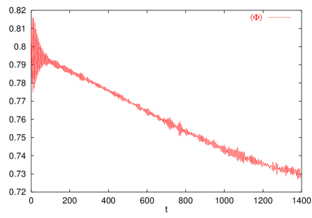
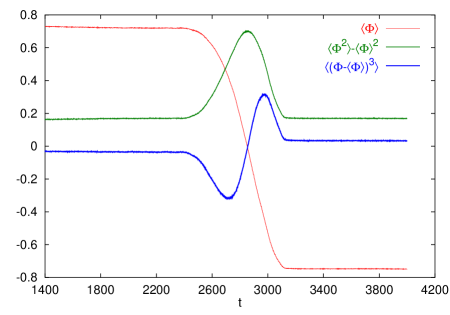
Figure 3.1: The time evolution of the order parameter, its MS fluctuation and the third moment. The example is selected from runs on a $N=512$ lattice with $h=-0.04/\sqrt{6}$ external source strength.

Figure 3.2: Early time power spectrum.

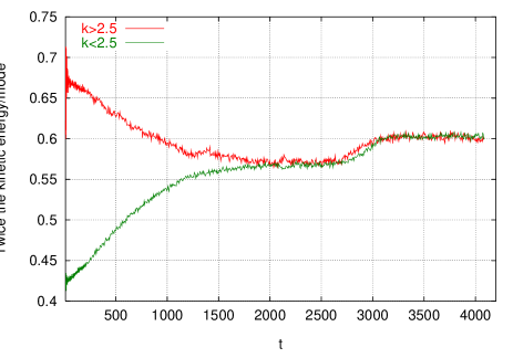
Figure 3.3: The time evolution of the kinetic energy content of the $|{\bf k}|>2.5$ and $|{\bf k}|<2.5$ regions averaged over the corresponding $|\bf{k}|$-intervals. The example is the same as in Fig. 1.

Next a slow, almost linear (modulated) decrease of the OP follows. At the same time its MS fluctuation increases linearly. In Fig.3.3 an energy flow towards the low-$|{\bf k}|$ part can be observed, which proceeds through the excitation of single modes in this part. As a result the minimum of the effective potential is continously shifted to smaller $\Phi$-values, as if the temperature would gradually increase (see the left part of Fig.3.1). The full (microscopic) kinetic energy density shows in this period less than 5% variation. In view of the picture based on the Maxwell construction it is rather surprising that independently of the initial conditions the OP converges towards a well-defined absolute value, depending only on the total energy density.

On the third portion the average value of the OP and its moments stay constant (see the right picture in Fig.3.1). The average energy content of the low and high-$|{\bf k}|$ part of the spectra is nearly the same. This suggests the establishment of a sort of thermal (meta)equilibrium.

In terms of the terminology introduced for the inflation, the first period leading to this (quasi) -stationary state can be called preheating, and the second reheating. Directly before the moment of the transition to the true vacuum a peak appears in the power spectrum in the narrow neighbourhood of ${\bf k}=0$ with varying position in time. On the snapshots of the real space configurations a set of randomly distributed small bubbles of the true ground state appear with a radius increasing in time, until one of the bubbles exceeds the critical size.

The fourth portion of the motion is the transition itself. The value of the OP MS-fluctuation increases by about a factor of three and the temporal width of this transient increase measures very well the transition time. The transition time decreases on larger lattices, the height of the jump in the OP-fluctuation is not sensitive to the lattice size. Also the third reduced moment shows a characteristic variation. An increase of the temperature proceeds smoothly during the transition of the OP to its stable value (Fig.3.3). The slight separation of the two curves in Fig.3.3 gives a feeling on the degree of uniformity of the temperature variation of the different modes.

The last portion of the trajectory represents stable (thermalised) oscillations around the true ground state. Here a complete equilibration of the power spectrum can be observed (see Fig.3.3) corresponding to a somewhat increased temperature $(T\sim 0.6)$.

3.2.3 Motion near the (meta)stable point

Our analysis of the motion around the (meta)stable value of the order parameter explores the consequences of assuming the ergodicity hypothesis for a sufficiently long finite time interval, after the system has already reached the equilibrium. The equilibrium is characterised by a limiting probability density in the configuration space. The averaging with this density should provide the same value as the one yielded by a single long time evolution when subsequent configurations are used in constructing the statistics. Our “statistical system” is now a single degree of freedom, the order parameter of the lattice system, interacting with all other ($k\neq 0$) modes.

The effective equation of motion can be thought to result from the application of a “molecular dynamical renormalization group”, to our microscopical equations. The blocking in space is performed by projecting the field configuration $\Phi({\bf x},t)$ on the OP $\Phi(t)$. It represents the infrared (IR) end point of such a blocking whose effective theory is now reconstructed from the actual time dependence found numerically. Combining ergodicity of the full system with the renormalization group (RG) concept we arrive to the conclusion that ensemble averages of any OP-function coincide with time averages of the same function.

In view of the RG concept we look for an effective equation of motion where the value of OP is determined exclusively by its values preceding in time. Assuming the absence of long memory effects a “gradient” expansion in time can be envisaged, leading to a local differential equation. We introduce into this phenomenological “Newton-type” equation a term violating time-reversal invariance. We are not able to derive it from the original system, we only wish to test its presence. The sustained motion of OP, however, requires, in this case the presence of a random “force” term, too. The deterministic part of the “force” is expected to be related to the equilibrium effective potential, since this object determines the stationary probability distribution for the OP near equilibrium.

The above considerations lead us to write down the equation of motion, which represents a linear relation between the acceleration and the velocity of the order parameter:

$$\ddot{\Phi}_{d}+\eta_{d}(\Phi_{d})\dot{\Phi}_{d}-h_{d}+{dV_{\textrm{eff}}(\Phi_{d})\over d\Phi_{d}}=\zeta_{d},$$ (3.48)

where $\zeta_{d}$ is a noise term. In the corresponding dimensionless equation of motion the following new rescaled quantities will appear:

$$\eta_{d}=|m|\eta,\qquad\zeta_{d}=\zeta|m|^{3}\sqrt{6\over\lambda}.$$ (3.49)

The fitting procedure for the coefficients on the left hand side of Eq. (3.48) was the following. For a given interval of time $I_{t}$ the region of the order parameter space visited by the system $\left\{\Phi(t)|t\in I_{t}\right\}$ was divided into small bins. Having defined the time set $T_{\Phi_{b}}=\left\{t\in I_{t}|\Phi_{b}<\Phi(t)<\Phi_{b}+\Delta\Phi\right\}$ corresponding to a given bin, the linear relation $\ddot{\Phi}(t_{b})=-\eta(\Phi_{b})\dot{\Phi}(t_{b})-f(\Phi_{b})$ was fitted with the method of least squares using the $\dot{\Phi}(t_{b})$, $\ddot{\Phi}(t_{b})$ data measured at time moments $t_{b}$ belonging to $T_{\Phi_{b}}$. We have obtained in this way the coefficient functions $\eta(\Phi_{b}),f(\Phi_{b})$. Once the functions $\eta(\Phi)$ and $f(\Phi)\equiv-h+V_{\textrm{eff}}^{\prime}(\Phi)$ are determined, we evaluate for each time $t$ the expression $\ddot{\Phi}(t)+\eta(\Phi(t))\dot{\Phi}(t)+f(\Phi(t))$. Its actual value determines the random noise function $\zeta(t)$, whose statistical features (autocorrelation) should be extracted from the data.

The effective force $f(\Phi)$ calculated from the time-average of the oscillatory motion around the equilibrium, is expected to agree with the force coming from the theoretically determined finite temperature effective potential calculated perturbatively in the cut-off two-dimensional field theory for some appropriately chosen value of the temperature [77]. With one-loop accuracy the expected equality reads:

$$f(\Phi)_{measured}=-h+{d\over d\Phi}\left[V(\Phi)+{T\over 8\pi}V^{{}^{\prime\prime}}(\Phi)\left(1+\log{\Lambda^{2}\over V^{{}^{\prime\prime}}(\Phi)}\right)\right]_{theory}+{\cal O}(T^{2}).$$ (3.50)

The expressions on the right hand side of this equation are connected to the dimensionfull quantities of the original one-loop computation in the following way:

$$T={\lambda\over 6|m|^{2}}T_{d},\quad V(\Phi)=-{1\over 2}\Phi^{2}+{1\over 4}\Phi^{4}={\lambda\over 6|m|^{2}}V_{d},\quad\Lambda={\pi\over a}.$$ (3.51)

The dimensionless temperature is defined by the time-average of the kinetic energy based on the assumption that in the effective theory of the OP it has the usual expression in terms of $\dot{\Phi}(t)$:

$$\lim_{t\rightarrow\infty}{1\over t}\int_{0}^{t}dt^{\prime}{1\over 2}(\dot{\Phi}(t^{\prime},x))^{2}\equiv{1\over 2}\overline{\dot{\Phi}^{2}}^{t}={T\over 2}.$$ (3.52)

One should note that this definition in the dimensionfull version implies a “Boltzmann-constant”, $|m|^{2}$ multiplying $T_{d}$.

By measuring the order parameter average for different values of the external field $h$ we obtain the magnetisation curve of the system. In the numerical work we restarted the computation at different values of the external magnetic field but one might as well change $h$ adiabatically and measure the force law at each (quasi)equilibrium point. The results should agree in the stable regime, up to the phenomenon of the hysteresis. The resulting curve can be viewed as the numerical Legendre transformation by identifying the external source $h$ with the derivative of the effective potential,

$$-h+V^{\prime}_{\textrm{eff}}(\langle\Phi\rangle_{h,measured})=0.$$ (3.53)

It was found that $f(\Phi)_{measured}$ is always vanishing at $\Phi=\langle\Phi\rangle_{h,measured}$, thus the force acting on the order parameter at the equilibrium position $\langle\Phi\rangle_{h}$ induced by the external source $h$ is indeed always $-V^{\prime}_{eff}(\langle\Phi\rangle_{h})$.

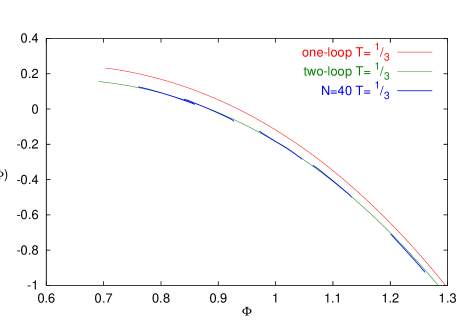
Figure 3.4: The force $f(\Phi)$ as the function of the order parameter on $40\times 40$ lattices with $T=1/30$ and $1/3$. The force is measured by shifting the center of motion to different $\Phi$ values by applying appropriate $h$ fields to the system. The finite size effects are negligible, see text. For comparison we display the force arising from the derivative of the one-loop and for $T=1/3$ also of the two-loop expressions of the effective potential.

The two sides of the relation (3.50) are shown in Fig.3.4. To the values of the external field used in preparing Fig.3.4 ($h\sqrt{6}=-0.5,-0.02,0,0.5,1,2)$ single runs were selected by the requirement that the system stayed in the metastable vacuum up to the time $10^{6}$. The force shown in Fig.3.4 demonstrates that not only the equilibrium positions but also the fluctuations of the OP are governed by the static effective potential. Similar measurements, performed on $100\times 100$ lattices showed no finite size effects in the stable regime, $h>0$. The error of $f(\Phi)$ is not shown in the Figure, since the typical values ($\sim 0.004$ for $T=1/3$ and $\sim 0.002$ for $T=1/30$) are too small to be displayed.

Another piece in the effective equation of motion (3.48) is the friction term whose presence indicates the dynamical breakdown of the time reversal symmetry. The friction coefficient $\eta(\Phi)$ proves clearly non-vanishing and shows only weak dependence on the actual value of the OP around its equilibrium position. The breakdown of the time-reflection symmetry in a closed system must arise only in presence of infinitely many degrees of freedom. Till then only statements on the Poincaré-time can be made. Thus our non-zero results for $\eta$ require further clarifications.

The point is that there are two types of infinities, controlled by the temporal UV and the IR cutoffs, respectively. The spontaneous symmetry breaking is driven by the IR modes, and the non-trivial minima of the potential energy arise from the presence of infinitely many degrees of freedom in the IR (thermodynamical limit). On the contrary, the dynamical symmetry breaking [78] is the result of the effects of the derivative terms in the action and the infinitely many UV modes (continuum limit). The breakdown of the time reversal, being related to a linear time-derivative term in the effective equation of motion, should come from the UV, the short time behaviour of the system.

In fact, one expects no friction when the UV cutoff, $a_{t}$ is so small, that not enough energy can be dissipated during such a short time. In quantitative terms one should have

$$a_{t}>\tau={2\pi\over\sqrt{{8\over a^{2}}+2}}+{\mathcal{O}}(T),$$ (3.54)

where $\tau$ is the time scale of the fastest mode in the system. The right hand side relation of Eq.(3.54) gives an estimate of the maximal frequency from the free dispersion relation $p_{0}^{2}=4(\sin^{2}p_{x}a/2+\sin^{2}p_{y}a/2)/a^{2}+M^{2}(T)$ of the lattice Hamiltonian system for fixed $a$ in the limit $a_{t}\to 0$. The fast modes absorb energy from the OP in a single time step for $a_{t}>\tau$, and the friction term should appear in the effective equation of motion.

Figure 3.5: The friction $\eta(\langle\Phi\rangle_{h=0})$ as the function of the timelike lattice spacing $b_{t}=na_{t}$. The time scale of the fastest mode is $\tau\approx 2$ and $0.22$ for $a=1$ and 0.1, respectively, according to the perturbation expansion. Typical error bars appear on the curves both for the IR and UV regimes.

With help of the temporal blocking

$$\Phi(t)\to\Phi_{n}(t)={1\over n}\sum_{k=-n/2}^{n/2-1}\Phi(t+ka_{t})$$ (3.55)

one can construct the trajectories $\Phi_{n}(t)$ corresponding to larger values of the time cut-off, $b_{t}=na_{t}$. Such blocking was performed in time up to $n=2000$ and a discrete time equation of motion of the form Eq.(3.48) was reconstructed for the blocked trajectory $\Phi_{n}(t)$. The non-trivial dependence of $\eta$ on the temporal cutoff $a_{t}$ is shown in Fig. 3.5.

One can distinguish two regimes separated by a crossover apparently independent of the lattice size, located at $b_{t}\approx 0.2\tau$. A scaling behavior is observed on the UV side, where $\eta(b_{t})$ tends to zero with a critical exponent close to 1 and the dissipative force being constant. This result should be independent of the actual blocking details. In the other regime, on the IR side $\eta$ goes over first into a $b_{t}$-independent regime, corresponding to the saturation of the energy transfer from the OP and giving a stable, microscopic definition of the friction coefficient. Finally, in the far IR part a qualitatively different oscillatory behaviour sets in.

The location of the crossover from the UV scaling regime to the plateau can be understood by writing the fluctuation dissipation theorem in the corresponding discretised form: $\langle\zeta^{2}\rangle=2\eta T/b_{t}$. The linearly increasing regime of $\eta(b_{t})$ implies constant second moment for the noise. When $\eta(b_{t})$ reaches the plateau the second moment of the noise decreases like $1/b_{t}$. The crossover therefore is located at the autocorrelation time scale of the noise.

A qualitative interpretation of the oscillatory IR regime can be based on the observed small amplitude beating phenomenon in the OP trajectory. This can be recognized by closer inspection of the left side of Fig.3.1, which persists further also on the right side. It is reflected in the OP autocorrelation function, too, since in the course of the blocking an interference effect occurs on the right hand side of Eq.(3.55) due to this regularity. This feature is relevant to the value of $\eta(b_{t})$, responsible for the decay of all kinds of fluctuations.

The appareance of peaks in $\eta(b_{t})$ at both the maximal destructive and constructive interferences can be modeled semi-quantitatively by identifying the beating part of the OP-motion ${\textrm{Re}}\delta\Phi={\textrm{Re}}\delta\Phi_{0}\exp(i\omega t)$ with the stationary solution of a single weakly damped driven harmonic oscillator, $\ddot{\delta\Phi}+\eta\dot{\delta\Phi}+\omega_{0}^{2}\delta\Phi=f_{0}\exp(i\omega t)$. The blocking acts on the trajectory $\delta\Phi(t)$ as $\delta\Phi(t)\to u\delta\Phi(t)$, where $u=(\exp(i\omega b_{t})-1)/i\omega b_{t}$. It does not change the relative phase of the driving force and of the blocked oscillation amplitude, leading to a relation between the parameters of the original and the blocked equation of motion:

$$-\omega^{2}+i\eta\omega+\omega_{0}^{2}=-\omega^{2}u^{2}+i\bar{\eta}\omega u+\bar{\omega}_{0}^{2}.$$ (3.56)

The friction coefficient for the blocked trajectory turns out to be $\bar{\eta}=(\eta+\omega\textrm{Im}(u^{2}))/\textrm{Re}(u)$. It is easy to see that $\textrm{Re}(u)$ is vanishing at maximal constructive and destructive interferences. This provides singularities in $\bar{\eta}$. Whenever $\textrm{Re}(u)=0$ we have $\textrm{Im}(u^{2})=0$ and numerator changes sign in the vicinity of the singularity. Thus $\bar{\eta}>0$ apart for a short time interval around the singularities where the non-harmonic features should stabilise the fluctuations and keep $\bar{\eta}>0$, as observed in our simulation.

The $a$ dependence appearing in Fig.3.5 arises from the following two effects. One is that for larger $a$ the maximal oscillation frequency is smaller and the time resolution of the system becomes cruder. Another is that larger $a$ represent bigger physical volume, many more soft modes and less harmonic system, which tends to invalidate the simple picture based on a single harmonic mode. As a result the effects of oscillatory nature will be smeared, as one clearly recognizes in the figure.

The quality of any proposed deterministic equation of motion (e.g. equations similar to Eq.(3.48) with zero on the right hand side), can be judged by the amplitude and the autocorrelation of its error term, the noise term $\zeta$. The amplitude of the noise was found at least two-three order of magnitude below the average level of the force as fitted to Eq. (3.48). The autocorrelation function of the noise of Eq. (3.48) appeared to be local, approximately of the form $\langle\zeta_{d}(t)\zeta_{d}(t^{\prime})\rangle\approx\delta^{\prime\prime}(t-t^{\prime})$. The status of the fluctuation-dissipation theorem will be investigated for more complex field theoretical systems in future investigations.

The selfconsistency of the definition of the temperature in Eq.(3.52) and also the establishment of the thermal equilibrium can be tested further by plotting histograms for the following quantities:

$$E_{k} = \frac{1}{2}\left({d\Phi\over dt}\right)^{2},$$

$$E_{p} = {\mu^{2}\over 2}(\Phi-\langle\Phi\rangle_{h})^{2},$$ (3.57)

$$E_{t} = E_{k}+E_{p},$$

where $\mu^{2}$ is the slope of the force as the function of the order parameter, determined numerically. Typical results for the energy-histograms are shown in Fig.3.6. It shows perfect agreement of all slopes and good agreement with the expectations based on equipartition of the energy between the kinetic and the potential parts. We have checked for several temperatures, that the temperature determined by these histograms and from the $|{\bf k}|$-spectra of the kinetic energy agree. This piece of information is parallel to the recent detailed investigations of the thermalisation in $(1+1)$-dimensional $\Phi^{4}$-theories [79, 80].

Figure 3.6: The histogram of the energies $E_{t}$, $E_{k}$ and $E_{p}$ of Eq.((3.2.3)) on a $256\times 256$ lattice with $h=2/\sqrt{6}$.

It is worthwhile noting that the relaxation from a given initial condition to the thermally distributed state like in this figure takes at least one order of magnitude longer time for systems in the symmetric phase compared to the spontaneously broken case. At higher energy density (temperature) one would expect larger collision frequency, therefore shorter thermalisation time. The opposite result hints to the importance of slow, soft modes, whose presence is due to the symmetry breaking mechanism. We shall argue in the next Subsection that these modes are responsible for the realization of the Maxwell-cut in the potential term of the effective equation of motion for the OP. What we find remarkable is that these modes are present not only in the mixed phase but also near (meta)stable equilibria, among the dynamical fluctuations around the ordered vacuum in contrast to the massive perturbative excitation spectrum in the equilibrium.

We complete the analysis of this subsection with the remark, that after the transition to the stable vacuum shortly a thermalised distribution is recovered for the OP at somewhat increased temperature which agrees with the value given by the equipartition.

3.2.4 Jump from the metastable to the stable vacuum

As it has been emphasized in the Introduction, there are (at least) two different descriptions of the transition from the metastable state to the stable one. In the first approach an expansion around the lower pass, the critical bubble (bounce) configuration yields a detailed space-time picture and the transition rate by means of the analytic continuation of the potential experienced by the OP near the (meta)stable position [65, 66].

Another possibility is to provide for the OP a probabilistic description, obtained by the elimination of all other degrees of freedom in some kind of blocking procedure. This description is based usually on some underlying Master equation for the probability distribution of the OP and the resulting Fokker-Planck equation [81]. The transition to the stable state appears in this approach formally as a tunneling solution of the Fokker-Planck equation. The probabilistic feature of the dynamics of the OP is supposed to arise from near the (meta)stable equilibrium assuming a statistical ensemble of the initial conditions.

In our simulation we find results analogous with the predictions of the probabilistic description by analysing the OP-motion starting from a single, well defined initial condition. One might wonder at this point if it is possible to understand the probabilistic tunneling of the OP by following the system from a unique initial condition. The self averaging in time can not be used for this argument since such a transition occurs only once during the evolution in a (quasi)irreversible manner. We have to develop a third approach to the metastable$\to$stable transition.

In general, the effective equation of motion for $\Phi(t)$ reflects the typical landscape of the microscopic potential energy functional around the actual point $\Phi({\bf x},t)$ in the configuration space. The classical origin of what appears as a tunneling on the Fokker-Planck level must be the arrival of $\Phi({\bf x},t)$ to the vicinity of some narrow valley opening up towards the stable vacuum. In traversing this valley the landscape changes and the typical fluctuations will be different from those felt in the metastable regime. The constants parametrising the effective equation of motion must reflect this change.

Our goal in this Subsection is to construct an effective description of the transition to the stable state by carefully tracing the time evolution of the OP. This will be achieved by projecting the microscopic equation of motion onto the homogeneous mode and phenomenologically parametrising it similarly to Eq.(3.48).

Figure 3.7: The force $f(\Phi)$ as the function of the order parameter on $100\times 100$ lattice with $h=-0.04/\sqrt{6}$. Each curve corresponds to time intervals of length $500|m|^{-1}$. The interval corresponding to the continous curve ends $1000|m|^{-1}$ before the transition, the long dashed curve refers to the next time interval and the short dashed curve is the force measured during the last time interval preceding the transition. One clearly observes the bending down left from the central OP-value in the metastable regime. Typical error bars are shown on the leftmost points of the three curves.

As long as the system is far from the narrow valley of the instability the force is time independent and agrees with the force derived from the perturbative effective potential according to the part of Fig. 3.4 corresponding to $\Phi>0.9$. When the system arrives close to the entrance of the unstable valley, $(\Phi\approx 0.8)$, the soft modes start to be important. This is reflected in the slight glitch in the leftmost piece of the measured force law in Fig. 3.4. A sequence of glitches results in a situation depicted in Fig. 3.7. It shows the force acting on the OP in three successive time intervals preceding the event of tunneling for $h=-0.04/\sqrt{6}$. The $f(\Phi)$ curves determined using Eq. (3.48) in the disjoint time subintervals coincide within error bars for all, but the last one. In this last interval preceding directly the transition towards the direction of negative $\Phi$ values, the fitted force bends down and its average becomes (a small positive) constant. This is characteristic feature of the instants when the system finds the entrance into the unstable potential valley. The vanishing of the force is an indication for the dynamical realization of the Maxwell-cut. The OP moves fast through the valley and the method of fitting the trajectory to Eq. (3.48) for finding the force fails due to the insufficient statistics.

The fluctuation moments depicted in Fig. 3.1 tell a bit more about this region. The increased values of the moments, the renormalized coupling constants in Wilsonian sense at vanishing momentum, indicate the enhanced importance of the soft interactions as the OP tunnels through the mean field potential barrier. This softening makes the OP fluctuating with larger amplitude. The valley of instability is in a surprising manner flatter than the typical landscape around equilibrium. The flatness along the motion of the OP (the mode ${\bf k}=0$ in momentum space) comes from the Maxwell-cut. The average curvature of the potential in the transverse directions, i.e. for modes with $|{\bf k}|\not=0$, can be estimated by the second functional derivative of the two dimensional effective action with cutoff $|{\bf k}|$, which can be taken as ${\bf k}^{2}+V^{\prime\prime}_{\bf k}(\Phi)$. The increased MS fluctuation of the OP corresponds to a decrease in $V^{\prime\prime}_{{\bf k}=0}(\Phi)$ in the valley. It pushes down $V^{\prime\prime}_{\bf k}(\Phi)$ also for small non-vanishing $|{\bf k}|$, in the low momentum regime which is expected to be the most influenced by the changing landscape.

The lesson of Fig. 3.7 is that the potential itself should be considered as a fluctuating quantity. This helps to translate into more quantitative terms the above qualitative points. We discuss the projection of the microscopic equation of motion (3.46) onto the zero momentum sector,

$$0=\ddot{\Phi}-\Phi+\Phi^{3}+3\overline{\varphi^{2}}^{V}\Phi+\overline{\varphi^{3}}^{V}-h\equiv\ddot{\Phi}+V_{\textrm{inst}}^{\prime}(\Phi),$$ (3.58)

where the symbol $\overline{\varphi^{n}}^{V}$ means the space average of $\varphi^{n}$, ($\overline{\varphi}^{V}=0,\Phi(t,{\bf x})=\Phi(t)+\varphi({\bf x},t)$). The instant potential introduced in the second line contains a deterministic piece, which is the sum of the tree-level potential and of the slowly varying part the second and third moments (eg. $(\overline{\varphi^{n}}^{V})_{det}$). This last feature clearly appears graphycally in Fig.3.1 and a simple model based on a two-phase model of the transition period will be constructed below to account for it. The remaining oscillating pieces of the moments provide the probabilistic fluctuating contribution to the instant potential:

$$V_{\textrm{inst}}(\Phi)=-h\Phi-\frac{1}{2}\Phi^{2}+{1\over 4}\Phi^{4}+(\overline{\varphi^{3}}^{V})_{det}\Phi+{3\over 2}(\overline{\varphi^{2}}^{V})_{det}\Phi^{2}+\zeta_{0}\Phi+{3\over 2}\zeta_{1}\Phi^{2}.$$ (3.59)

The additive ($\zeta_{0}$) and the multiplicative ($\zeta_{1}$) noises are given by the differences

$$\zeta_{0}(t) = \overline{\varphi^{3}}^{V}(t)-(\overline{\varphi^{3}}^{V})_{det},$$

$$\zeta_{1}(t) = \overline{\varphi^{2}}^{V}(t)-(\overline{\varphi^{2}}^{V})_{det}.$$ (3.60)

Note that no friction terms can be introduced in a natural way into the system (3.58-3.60). Therefore we face the intriguing question, how irreversibility is realised in such a system. The time-correlation matrix $\overline{\zeta_{i}(t)\zeta_{j}(t+\tau)}^{t}$ appears to us to be the key object for its investigation, to which we plan to return in the future.

In order to gain more insight how this works we build into Eq.(3.58) the consequences of the mixed two-phase picture of the phase transformation. The microscopical basis for this picture is provided by the thermal nucleation whose quantitative discussion is given in the Subsection 3.2.5.

More specifically, we assume that the space can be splitted into sharp domains (neglecting the thickness of the walls in between), where the field is the sum of the constant background values $\Phi_{0\pm}$ and the fluctuations $\tilde{\varphi}_{\pm}$ around it,

$$\Phi_{\pm}({\bf x},t)=\Phi_{0\pm}+\tilde{\varphi}_{\pm}({\bf x},t).$$ (3.61)

We assume local equilibrium in both phases, based on the smooth evolution of the temperature as displayed in Fig.3.3.

The actual value of the order parameter is determined by the surface ratio $p(t)$ occupied by the stable phase:

$${\Phi(t)}=p(t)\Phi_{0-}+(1-p(t))\Phi_{0+}.$$ (3.62)

Simple calculation then yields

$$(\overline{\varphi^{2}}^{V})_{det}(t) = \frac{\Phi_{0+}-\Phi(t)}{\Phi_{0+}-\Phi_{0-}}\left(\overline{\Phi_{-}^{2}({\bf x},t)}^{V}-\overline{\Phi_{+}^{2}({\bf x},t)}^{V}\right)+\Phi_{0+}^{2}-\Phi^{2}(t)+\overline{{\tilde{\varphi}_{+}}^{2}}^{V},$$ (3.63)

$$(\overline{\varphi^{3}}^{V})_{det}(t) = \frac{\Phi_{0+}-\Phi(t)}{\Phi_{0+}-\Phi_{0-}}\left(\overline{\Phi_{-}^{3}({\bf x},t)}^{V}-\overline{\Phi_{+}^{3}({\bf x},t)}^{V}\right)$$ (3.64)

$$+\overline{\Phi_{+}^{3}({\bf x},t)}^{V}-3\Phi(t)(\overline{\varphi^{2}}^{V})_{det}(t)-\Phi^{3}(t),$$

where the volume averages should be read off the corresponding equilibria on the two sides of the transition. If one takes the values of $\Phi_{0\pm},\overline{\tilde{\varphi}^{n}_{\pm}}^{V}$ from the respective equilibria determined in the same simulation, a quite accurate description of the shape of the two fluctuation moments arises in the whole transition region and its close neighbourhood using $\Phi(t)$ to parametrize their $t$-dependence. (Note that $\overline{\Phi^{n}_{\pm}(x,t)}^{V}$ does not depend on time.) The deterministic part of the moments are therefore well-defined functions of $\Phi$. In this way, a simple explicit construction can be given for the effective noisy equation of the OP-motion, if the above pieces are supplemented by the correlation characteristics of the two kinds of noises.

The RMS (root mean square) fluctuations found numerically on the transition part of the trajectory and its close neighbourhood are the following:

$$\sqrt{\overline{\zeta_{0}^{2}(t)}^{t}}=0.0063(10),\quad\sqrt{\overline{\zeta_{1}^{2}(t)}^{t}}=0.0054(10),\qquad\textrm{for}\,N=64$$ (3.65)

(its magnitude increases with the size of the system). The magnitude of their equilibrium cross correlation was found $\sim 10^{-5}$.

As a corollary of this construction one can demonstrate the absence of the deterministic part of the acceleration of the order parameter in the transition period.

Substituting Eqs.(3.63), (3.64) into Eq.(3.58), one finds for the deterministic part of the force,

$$f\left(\Phi\right)=\left(-1+\frac{\overline{\Phi_{+}^{3}({\bf x},t)}^{V}-\overline{\Phi_{-}^{3}({\bf x},t)}^{V}}{\Phi_{0+}-\Phi_{0-}}\right)\Phi+\frac{\Phi_{0+}\overline{\Phi_{-}^{3}({\bf x},t)}^{V}-\Phi_{0-}\overline{\Phi_{+}^{3}({\bf x},t)}^{V}}{\Phi_{0+}-\Phi_{0-}}-h.$$ (3.66)

The average of the equations of motion in the respective equilibria,

$$\langle\Phi_{\pm}^{3}({\bf x},t)\rangle-\Phi_{0\pm}-h=0$$ (3.67)

implies the vanishing of the deterministic force in Eq. (3.66), when exploiting the equality of the volume and the ensemble average in this case. Eq. (3.58) transforms into

$$\ddot{\Phi}(t)+\zeta_{0}(t)+3\zeta_{1}(t)\Phi(t)=0.$$ (3.68)

This is the dynamical realization of the Maxwell-construction holding when the mixed phase model with local equilibrium is valid.

If the force is calculated from the full instant potential, $V(\Phi)_{\textrm{inst}}$ in Eq. (3.59), it depends parametrically on the moments $\overline{\varphi^{2}}^{V}(t)$ and $\overline{\varphi^{3}}^{V}(t)$. The approximate trajectory $\Phi_{\textrm{inst}}(t)$, defined by minimising $V(\Phi)_{\textrm{inst}}$ with respect to $\Phi$, where the moments are taken from the numerically determined time evolution, reproduced accurately the observed OP, $\Phi(t)$ with the following RMS/unit time:

$$\sqrt{\overline{(\Phi(t)-\Phi_{\textrm{inst}}(t))^{2}}^{t}}=0.0014(5),\qquad\textrm{for}\,N=64.$$ (3.69)

This construction interpretes the OP-trajectory as a continous deformation of the instant potential with the OP “sitting” permanently in the actual minimum. Notice that such motion is possible only if the OP continously undergoes some sort of dissipation.

The vanishing of the acceleration was checked by comparing the computer generated OP trajectory in the transition region with a ballistic motion in a viscous medium. In particular it was tested that the ratio $h/\dot{\Phi}$ is nearly time and $h$ independent for small enough $h$. The dynamical friction measured by the above ratio tends to a constant with decreasing $h$ at fixed lattice size. Although the error for its value in each individual transition is rather small, the central values obtained in different runs fluctuate quite strongly, which leads eventually to a large error of the mean calculated as an average of runs with different initial configurations having the same energy density.

It is worth to note that the order of magnitude of these “renormalized”, i.e. IR determined values of the friction coefficient agree with the peak value in Fig. 3.5 for $N=64$. The “running” friction coefficient determined by the blocking in time, however, drops as $b_{t}$ is increased and takes extremely small values at $b_{t}\approx 20$, the average time length of the ballistic fits for the transition. This serves an example for the dependence of the renormalization group flow on the details of the blocking. It remains to be understood whether the agreement between the peak value and the ballistic fit is an accident or follows from the internal dynamics.

3.2.5 Connection with the nucleation picture

In this subsection we analyse the transition using the more conventional statistical approach of thermal nucleation theory.

From the study (on lattices up to $N=512$) of the detailed microscopical field configurations it turned out that the phase transformation starts by the nucleation of a single bubble of the stable ($\Phi<0$) phase. Late-coming further large bubbles are aggregated to it as well as the small size (consisting of $n_{bubble}<50-60$ joint sites) bubbles. Following the nucleation the expansion rate of the large bubble governs the rate of change of the order parameter. To a very good approximation each individual transition could have been characterised by a constant value of $\dot{\Phi}$ in this interval. Two mechanisms are known to lead to this behavior. The first is scattering of hard waves (“particles”) off the bubble wall, while in the second the expansion velocity is limited by the diffusive aggregation of smaller bubbles [82]. The latter process seem to be the dominant in the kinetic Ising model [83].

Figure 3.8: The normalised “release” time histogram counting the frequency of a certain time moment-bin when the order parameter first takes a negative value. The figure represents the statistics based on 750 events at $h=-0.08/\sqrt{6}$ on an $N=64$ lattice.

The statistics of the “release” time of the supercritical bubble from the metastable state shows at first sight rather peculiar characteristics. The binned histogram for larger values of $h$ shows an asymmetric peaked structure which apparently deviates from the exponential distribution characterising the thermal nucleation scenario (Fig.3.8). The very early transitions ($t<t_{max}$) seem to be suppressed for small values of $h$. We expect they correspond to transitions, which happen before the system reaches the metastable state.

The fall-off for $t>t_{max}$ starts nearly exponentially, but the histogram develops a very long tail when $h\rightarrow 0$. The bigger sample is used for estimating the probability distribution, the more suppressed is the weight of these events in the normalised distribution. In practice this means a longer time interval where a good linear fit can be obtained to the log-linear histogram. Eventually, the separation of a clean exponential signal is possible, and the slope can be compared with predictions of the nucleation theory.

Knowing the frequency histogram of the time $t$ that elapsed before the system has escaped from the metastable region by nucleating a growing bubble of the stable state, we can construct the nucleation rate per unit area: $\Gamma(h)$. Indeed, for a lattice size $L$ we can read off $\Gamma$ by fitting to the expected form $P_{h}(t)\sim exp(-t\Gamma(h)L^{2})$.

The nucleation rate is proportional to the volume of the system $L$. In Fig.3.9 we see evidence for the size independence of the transition rate per unit surface. The logarithm of this quantity can be estimated following the standard nucleation theory [65, 66, 84] where the nucleation rate per unit area is given by:

$$\Gamma\sim e^{-S_{2}/T},\qquad\textrm{with}\qquad S_{2}=S(\Phi_{B})-S(\Phi_{f}(h)),$$ (3.70)

$\Phi_{B}$ is the bounce solution and $S$ the Euclidean action $S=\int d^{2}x\left[\frac{1}{2}(\partial_{\mu}\Phi)^{2}+U(\Phi)\right]$ with $U(\Phi)$ defined below in Eq. (3.74).

Figure 3.9: Nucleation rate for unit lattice surface versus the reciprocal of the magnetic field for different lattice sizes. The error bars are smaller than the size of the symbols representing the data points.

In the so called thin wall approximation, when the energy density difference beween the true and the false vacuums is tiny the coefficient $S_{2}$ can be calculated analiticaly and in the relation

$$\ln\Gamma=K-{S_{2}\over T}.$$ (3.71)

$S_{2}$ is determined approximately by the action of the bounce solution, connecting the two vacua. In the investigation below we have studied at fixed temperature the $h$-dependence of $S_{2}/T$, assuming the $h$-independence of $K$, although this might be not the case.

The bounce is a solution of the Euclidean Euler-Lagrange equation of a theory defined by the action $S(\Phi)=\int d^{2}r\left(\frac{1}{2}(\nabla\Phi)+\frac{1}{2}m^{2}\Phi^{2}+\frac{\lambda}{24}\Phi^{4}+h\Phi\right)$ such that (see fo exemple [66])

1. $\Phi_{B}$ approaches the false vacuum $\Phi_{f}(h)$ at the infinity,

2. $\Phi_{B}$ is not a constant,

3. $S(\Phi_{B})$ is the minimal amoung the solutions obeying 1. and 2.  .

Since the nucleation proceeds through approximately spherical bubbles we need an $O(2)$-invariant solution of the equation of motion i.e. the solution of

$$\frac{d^{2}\Phi}{dr^{2}}+\frac{1}{r}\frac{d\Phi}{dr}=m^{2}\Phi+\frac{\lambda}{6}\Phi^{3}+h,$$ (3.72)

with the boundary conditions ensuring that the field be regular at the origin ($\Phi^{\prime}_{B}(0)=0$) and in the false vacuum at spatial infinity ($\Phi_{B}(\infty)=\Phi_{f}(h)$).

As it is well-known, in the thin wall approximation the differential equation (3.72) reduces to

$$\frac{d^{2}\Phi}{dr^{2}}=\frac{dU_{+}(\Phi)}{d\Phi},$$ (3.73)

where $U_{+}(\Phi)$ is the a symmetric function of $\Phi$, with minima at $\Phi_{f,t}=\pm\sqrt{\frac{6}{\lambda}}|m|$, obtained by replacing $h$ by $0$ in the tree level potential of Lagrangian and dropping the constant term:

$$U(\Phi)=\frac{1}{2}m^{2}\Phi^{2}+\frac{\lambda}{24}\Phi^{4}+h\Phi=\underbrace{\frac{\lambda}{24}\left(\Phi^{2}+6\frac{m^{2}}{\lambda}\right)^{2}}_{U_{+}(\Phi)}+h\Phi-\frac{3}{2}\frac{m^{4}}{\lambda}$$ (3.74)

Multiplying equation (3.73) by $\Phi^{\prime}$ one can see that it admits a first integral $\left[\frac{1}{2}(\Phi^{\prime})^{2}-U_{+}\right]^{\prime}=0,$ whose value is determined by the condition that $\Phi(\infty)=\Phi_{f}$ and $\frac{d\Phi}{dr}\Bigl{|}_{\infty}=0$ because of the finiteness of the energy. So, we have

$$\frac{1}{2}(\Phi^{\prime})^{2}-U_{+}(\Phi)=-U_{+}(\Phi_{f})=0.$$ (3.75)

This equation determines a monotonic $\Phi$ which goes from $\Phi_{t}$ to $\Phi_{f}$. The solution depends on a single integration constant $\bar{r}$, a point at which the $\Phi$ takes the average of its two extreme values $\Phi_{t}$ and $\Phi_{f}$:

$$\int_{0}^{\Phi}\frac{d\bar{\Phi}}{\sqrt{2\left[U_{+}(\bar{\Phi})-U_{+}(\Phi_{f})\right]}}=r-\bar{r}.$$ (3.76)

Performing the integral we obtain the well-known kink solution

$$\Phi(r)=|m|\sqrt{\frac{6}{\lambda}}\tanh\left[\frac{|m|}{\sqrt{2}}(r-\bar{r})\right].$$ (3.77)

Expressed analytically the thin wall approximation of the bounce looks like:

$$\Phi_{B}(r)=\left\{\begin{array}[]{ll}\Phi_{t},&0<r<\bar{r}-\Delta r\\ \Phi_{wall}(r),&\bar{r}-\Delta r<r<\bar{r}+\Delta r\\ \Phi_{f},&r>\bar{r}+\Delta r\end{array}\right.$$ (3.78)

which describes a bubble of radius $\bar{r}$ of the stable phase $\Phi_{t}$ embedded in the metastable phase $\Phi_{f}$. $\Phi_{wall}(r)=|m|\sqrt{\frac{6}{\lambda}}\tanh\left[\frac{|m|}{\sqrt{2}}(r-\bar{r})\right]$ describes the bubble wall separating the two phases.

The unknown parameter $\bar{r}$, the radius of the ball, can be determined by computing the action in the above approximation and demanding that it be stationary under variations of $\bar{r}$. We have to calculate the action in three distinct regions according to the solution (3.78).
Outside the wall, $\Phi=\Phi_{f}$ hence, ${S_{2}}_{outside}=0$.
Inside the wall, $\Phi=\Phi_{t}$ hence, ${S_{2}}_{inside}=2\pi\frac{\bar{r}^{2}}{2}h\left(\Phi_{t}-\Phi_{f}\right)=2\pi\bar{r}^{2}h\Phi_{t}-=-2\pi\bar{r}^{2}h\sqrt{\frac{6}{\lambda}}|m|$.
Within the wall, in the thin-wall approximation,

$${S_{2}}_{wall} = 2\pi\bar{r}\int dr\left[\frac{1}{2}{\Phi^{\prime}}_{wall}^{2}+U_{+}(\Phi_{wall})-U_{+}(\Phi_{f})\right]$$ (3.79)

$$= 2\pi\bar{r}\int_{\Phi_{t}}^{\Phi_{f}}d\Phi_{wall}\sqrt{2U_{+}(\Phi_{wall})}=:2\pi\bar{r}S_{1}.$$

So, we can conclude that the action asscociated with the bounce in the thin-wall approximation is:

$$(S_{2})_{d}=-2\pi\bar{r}^{2}h\sqrt{\frac{6}{\lambda}}|m|+2\pi\bar{r}S_{1},$$ (3.80)

where the $S_{1}$ is the energy of the kink

$$S_{1}=\int dr\left[\frac{1}{2}{\Phi^{\prime}}_{wall}^{2}+U_{+}(\Phi_{wall})\right]=3\frac{|m|^{4}}{\lambda}\int_{-\infty}^{\infty}dr\frac{1}{\cosh^{4}\left(\frac{r|m|}{\sqrt{2}}\right)}=4\sqrt{2}\frac{|m|^{3}}{\lambda}.$$ (3.81)

The first term on the right hand side of Eq. (3.80) corresponds to the volume energy of a bubble of radius $\bar{r}$, the second one to its surface energy.

From the stationarity of $S_{2}$ with respect of the variation of $\bar{r}$ ($\frac{dS_{2}}{d\bar{r}}=0$) we can calculate $\bar{r}$:

$$\bar{r}=\frac{S_{1}}{2h|m|}\sqrt{\frac{\lambda}{6}}=\frac{2}{h\sqrt{3}}\frac{|m|^{2}}{\sqrt{\lambda}}.$$ (3.82)

For the critical bubble size a very simple expression is obtained for the exponent of the rate in terms of dimensionless quantities:

$${S_{2}(\textrm{thin~{}wall})\over T}={16\pi\over\sqrt{6}}{|m|^{5}\over\lambda^{3/2}}{1\over h_{d}T_{d}}={4\pi\over 9}{1\over hT}.$$ (3.83)

The linear dependence on $1/h$ is fulfilled in our numerical calculations very well, but the predicted action is more than one order of magnitude larger than what can be derived from the slope of Fig.3.9: $S_{2}/T(\textrm{measured})\approx 0.1/(hT)$. If one relaxes the thin wall approximation and solves numerically the two-dimensional bounce equation directly for several $h$, one finds $S_{2}(\textrm{bounce})/T=0.78/(hT)$.

We mention here that for finding the bounce solution we have to choose an initial value for $\Phi>{\Phi}_{min}(h)$ evolve it and see what’s happening at a later $x$. If $\Phi>{\Phi}_{max}(h)$ then the solution overshoots and if $\frac{d\Phi}{dx}<0$ then the solution undershoots. We have to tune the initial value of $\Phi$ and the steps of the fourth order Runge-Kutta algorithm we used, in order to achieve that the solution stays very close to ${\Phi}_{max}(h)$, as long as possible. . Given the bounce solution we can simply evaluate its action by performing a numerical integration .

Further improvement can be obtained by applying the temperature corrected effective potential in the bounce equation. We have determined the parameters of the $T$-dependent potential directly from our numerical calculation in the following way. The restoring force was measured for a certain $h$ around both the stable and the metastable minima as described in Subsection 3.2.3. Next an interpolating fit has been constructed of the form: $h_{\textrm{eff}}+m^{2}_{\textrm{eff}}\Phi+\lambda_{3}\Phi^{2}+\lambda_{\textrm{eff}}\Phi^{3}/6$. It turned out that in the best fit $\lambda_{3}\approx 0$ is fulfilled always, while the values of the other coefficients are not too far from their tree level values. Then a bounce solution can be built on the corresponding (real!) potential which includes the temperature corrections. The final result is quite close to the measured value of the rate logarithm: $S_{2}(T,\textrm{bounce})/T=0.29/(hT)$. The same real interpolation can be built on the neighbourhood of the minima of the 2-loop $T$-dependent effective potential, leading to $S_{2}(T,\textrm{bounce})/T=0.2/(hT)$. By common experience in the surface tension simulations a factor of 2-3 difference in $S_{2}$ is expected to arise relative to the mean field theory.

We conclude, that the finite temperature corrections are important for quantitative treatment of the nucleation rate within the thermal nucleation theory.

Next we turn to the discussion of the possible nucleation threshold at small $h$. The average “release time” increases for fixed lattice size with decreasing $h$ (Fig.3.10). On a lattice of fixed size we found small $h$ values for which we could not detect any transition, what makes very probable the existence of a threshold value of the external field $h_{th}(N)$. We did not attempt to locate this value beyond the simple hyperbolic fits to the few largest $\langle t_{release}\rangle$ values. The value of $h_{th}(N)$ remains stable when the smallest $h$ is excluded from the fit, therefore we conclude that a threshold magnetic field exists similar to the case of the kinetic Ising model [83]. The value of $h_{th}$ decreases when the lattice size is increased. Intuitively we expect $h(\infty)=0$, but with the three lattices studied by us this conjecture cannot be demonstrated.

Figure 3.10: The average “release” time as a function of $h$ measured on $N=64,128,256$ lattices.

3.2.6 Conclusions

In this Section we have investigated in detail the decay of the false vacuum in a classical lattice field theory. This serves as a demonstrative example of the nonlinear relaxation of a far out of equilibrium classical cut-off field theory. Our investigation was based dominantly on the effective theory of the order parameter. Two versions of the effective theory were reconstructed from its trajectory derived from the microscopical equations of the theory. The first refers to the (meta)stable branch of the motion. The second one which takes into account the existence of a mixed phase during the transition period describes very well the transition together with its neighbourhood. The first equation has the form of conventional mechanical motion taking place in a dissipative noisy environment. The dissipation, the dynamical breakdown of the time reversal symmetry was found only for times longer than the minimal microscopic time scale of the system, the autocorrelation time of the noise.

Our results offer a“dualistic” resolution of the competition between the nucleation and the spinodal phase separation mechanisms in establishing the true equilibrium. On the one hand, we find that the statistical features of the decay of the false vacuum agree with the results obtained by expanding around the critical bubble. The microscopic mapping of the field configurations during the relaxation supports the bubble creation scenario. Alternatively, the effective OP-theory displays the presence of soft modes and produces dynamically a Maxwell-cut when the time dependence of the transition trajectory is described in the effective OP theory. We find that the larger is the system the smaller is the external field which is able to produce the instability. For infinite systems an infinitesimal field pushes the system through the Maxwell-cut, where no force is experienced by the OP. Therefore it will not stop before reaching the true homogenous ground state passing by the mixed states with constant velocity.

Chapter 4 The damping of the Goldstone modes

This Chapter is devoted to the dynamics of the Goldstone modes. First we derive a set of effective equations for the long-wavelength modes of an $O(N)$ symmetrical scalar field theory. Next, we analytically determine the damping rate of the Goldstone modes as a function of the wave number $\bf k$. Next, in an $O(2)$ symmetrical scalar field theory we determine the same rate in the presence of a small explicit symmetry breaking parameter $h$. We study the behaviour of the damping rate as $h\rightarrow 0$.

By performing a $2+1$ dimensional numerical simulation in an $O(2)$ symmetric classical field theory, we check the large time asymptotic power law of the relaxation of an arbitrary field configuration. The manifestation of Mermin–Wagner theorem is also discussed.

4.1 Effective theory for the soft modes in O(N) $\Phi^{4}$ model

In this section we extend our discussion to the broken phase dynamics of the N-component scalar field theory with $\Phi^{4}$ self-interaction. This model is relevant to the dynamics of the $\pi-\sigma$-system $(N=4)$ [85] and is actively investigated in connection with the phenomenon of the disoriented chiral condensate [86, 87, 88, 89]. The appearance, the evolution and the damping of the low frequency fluctuations and instabilities of the chiral order parameter are carefully studied in these papers. Less attention is paid to the damping of the Goldstone-modes. Though in the realistic case the explicit breaking of the $O(N)$ symmetry leads to massive “Goldstone”-bosons, it is of interest to see what is the intrinsic dynamics of these excitations in the “ideal” spontaneously broken case. It turns out that the damping of the Goldstone-fluctuations with frequency $k_{0}$ is essentially different in the respective domains

$$k_{0}\ll{M^{2}\over T}\ll M<T,\qquad\textrm{and}\qquad{M^{2}\over T}\ll k_{0}\ll M<T.$$ (4.1)

Our conclusion is that both the on-shell dissipation time and the large time asymptotics of the Goldstone fields is qualitatively different in the first region in comparison to the fluctuations of the order parameter.

The physical picture is very appealing. Radial fluctuations along the order parameter relax fairly quickly, what freezes fast the length of the vacuum expectation value of the $\Phi$ field. The second stage of the relaxation consists of the slow rotation of the order parameter, which is described by the relaxation of collectively excited low momentum Goldstone fluctuation modes.

The high-temperature one-loop quantum dynamics of scalar models has been investigated very actively recently partly as a kind of theoretical laboratory for developing powerful calculational methods, partly with the aim to provide answers to important questions of inflatory cosmology and the physics of heavy ion collisions. Our work was substantially influenced by References [60, 90, 91, 25, 92].

We first derive in Subsection 4.1.1 the effective equations for the low frequency modes. The coefficients of the terms correcting the classical equations are determined by various $n$-point functions of the fast modes. For the effective dynamics we work out the modification of the linear part of the equations (the self-energy operator), which is fully determined by the two-point function of the high-frequency fields. A detailed study of this quantity appears in Subsection 4.1.2. Stated in more technical terms, we compute one-loop contributions to the two-point functions with full $T=0$ propagators and restrict the temperature dependent contribution to the $p_{0}>\Lambda$ modes. This approach follows the finite temperature renormalization group transformation scheme of D’Attanasio and Pietroni [59]. In Subsection 4.1.3 we shall discuss, in particular, whether the linear response of the high frequency modes to long wavelength fluctuations allows a classical kinetic theory interpretation. Using the results obtained for the two-point function of the theory, in Subsection 4.1.6 we present the explicit effective field equations, with help of auxiliary fields introduced to handle the nonlocal nature of the effective dynamics. Our results are summarised in Subsection 4.1.7. In Appendix B some results of the main text are rederived with help of the conventional perturbation theory in a form explicitly showing its equivalence to the Dyson-Schwinger treatment. Appendix C presents the iterative solution of the dynamics of the classical $O(N)$-model. Some relevant integrals are explicitly evaluated in Appendix D.

4.1.1 The effective equations of motion for the slow modes

The Lagrangian of the system is given by

$$L={1\over 2}(\partial_{\mu}{\bf\Phi}_{a})^{2}-{1\over 2}m^{2}({\bf\Phi}_{a})^{2}-{\lambda\over 24}(({\bf\Phi}_{a})^{2})^{2}.$$ (4.2)

The aim of this investigation is to integrate out the effect of $p_{0}>\Lambda$ high frequency fluctuations. From the point of view of the final result it turns out to be important whether $\Lambda<M$ or $\Lambda>M$, where $M$ is the mass scale spontaneously generated in the broken symmetry phase. In the spirit of the renormalization group the value of $\Lambda$ will be lowered gradually and the importance of passing the scale $M$ will become evident in this process. Our actual interest will concentrate on the temporal variation of the lowest frequency fluctuations $k_{0}\ll\Lambda$.

We separate in the starting Lagrangian the high-frequency modes ($\varphi_{a}(x)$ with frequency $\omega>\Lambda$) and the low-frequency modes ($\tilde{\phi}_{a}(x)$ with frequency $\omega<\Lambda$)

$${\bf\Phi}_{a}(x)\rightarrow\tilde{\phi}_{a}(x)+\varphi_{a}(x).$$ (4.3)

Averaging over the high frequency fluctuations gives $\langle\varphi_{a}(x)\rangle=0$ which yields also $\tilde{\phi}_{a}(x)=\langle{\Phi_{a}(x)}\rangle$. This separation leads to

$$L = {1\over 2}(\partial\tilde{\phi}_{a})^{2}+{1\over 2}(\partial\varphi_{a})^{2}-{m^{2}\over 2}\Bigl{[}(\tilde{\phi}_{a})^{2}+(\varphi_{a})^{2}\Bigr{]}-{\lambda\over 24}\Bigl{[}(\tilde{\phi}_{a})^{2}(\tilde{\phi}_{b})^{2}+(\varphi_{a})^{2}(\varphi_{b})^{2}\Bigr{]}$$ (4.4)

$$-{\lambda\over 24}\Bigl{[}4(\tilde{\phi}_{a}\varphi_{a})(\tilde{\phi}_{b}\varphi_{b})+4(\tilde{\phi}_{a}\varphi_{a})(\varphi_{b})^{2}+4(\tilde{\phi}_{a}\varphi_{a})(\tilde{\phi}_{b})^{2}+2(\tilde{\phi}_{a})^{2}(\varphi_{b})^{2}\Bigr{]}.$$

From Eq.(4.4) the equations for the slow modes can be derived:

$$(\partial^{2}+m^{2})\tilde{\phi}_{a}+{\lambda\over 24}\left[8\varphi_{a}(\tilde{\phi}_{b}\varphi_{b})+4\tilde{\phi}_{a}(\tilde{\phi}_{b})^{2}+4\varphi_{a}(\varphi_{b})^{2}\right.$$

$$\left.\qquad\qquad\qquad\qquad\qquad+4\varphi_{a}(\tilde{\phi}_{b})^{2}+8\tilde{\phi}_{a}(\tilde{\phi}_{b}\varphi_{b})+4\tilde{\phi}_{a}(\varphi_{b})^{2}\right]=0.$$ (4.5)

The effect of the high-frequency fluctuations on the slow ones is obtained by averaging the equations with respect to their statistics. At one-loop level accuracy $\langle\varphi_{a}\varphi_{b}\varphi_{c}\rangle=0$ and one arrives at

$$(\partial^{2}+m^{2})\tilde{\phi}_{a}+{\lambda\over 6}\tilde{\phi}_{a}(\tilde{\phi}_{b})^{2}+{\lambda\over 3}\tilde{\phi}_{b}\langle\varphi_{a}\varphi_{b}\rangle+{\lambda\over 6}\tilde{\phi}_{a}\langle(\varphi_{b})^{2}\rangle=0.$$ (4.6)

We introduce at this point the conventional notation:

$$\Delta_{ab}(x,y)\equiv\langle\varphi_{a}(x)\varphi_{b}(y)\rangle.$$ (4.7)

Below no summation will be understood when repeated indices appear without the explicit summation symbol. We shall also use specific pieces extracted from the above two-point functions defined as

$$\Delta^{(0)}_{ab}(x,y)\equiv\Delta_{ab}(x,y)|_{\tilde{\phi}=0},\qquad\Delta^{(1)}_{ab}(x,y)\equiv\int dz{\delta\Delta_{ab}(x,y)\over\delta\tilde{\phi}_{c}(z)}|_{\tilde{\phi}=0}\cdot\tilde{\phi}_{c}(z).$$ (4.8)

In the broken symmetry phase one has to separate the nonzero average value from the slowly varying field, and write the equation only for the fluctuating part:

$$\tilde{\phi}_{a}\rightarrow\bar{\phi}\delta_{a1}+\phi_{a},$$ (4.9)

where we have chosen the direction of the average to point along the $a=1$ direction. We shall analyse the resulting equations for the $a=1$ and the remaining $a=i\neq 1$ components separately. Since the main effect of the high frequency modes we are interested in is the modification of the mass term (self-energy contribution), therefore we shall restrict our study to the linearised equation of $\phi_{a}(x)$. One has to take into account that the two-point functions $\langle\varphi_{a}\varphi_{b}\rangle$ depend on the background $\phi_{a}(x)$. For the linearised equations it is sufficient to compute them only up to terms linear in the background.

The two equations are

$$(\partial^{2}+{\lambda\over 3}\bar{\phi}^{2})\phi_{1}(x)+\frac{\lambda\bar{\phi}}{2}\phi_{1}^{2}(x)+\frac{\lambda\bar{\phi}}{6}\sum\limits_{i\neq 1}\phi_{i}^{2}(x)+\frac{\lambda}{6}\phi_{1}(x)\sum\limits_{a}\phi_{a}^{2}(x)+J_{1}(x)=0,$$

$$\partial^{2}\phi_{i}(x)+\frac{\lambda\bar{\phi}}{3}\phi_{i}(x)\phi_{1}(x)+\frac{\lambda}{6}\phi_{i}(x)\sum\limits_{a}\phi_{a}^{2}(x)+J_{i}(x)=0,\qquad(i\neq 1)$$ (4.10)

with the induced currents

$$J_{1}(x) = {\lambda\over 2}\bar{\phi}\Delta^{(1)}_{11}(x,x)+{\lambda\over 6}(N-1)\bar{\phi}\Delta^{(1)}_{ii}(x,x),$$

$$J_{i}(x) = {\lambda\over 3}\left(\Delta^{(0)}_{ii}(x,x)-\Delta^{(0)}_{11}(x,x)\right)\phi_{i}+{\lambda\over 3}\bar{\phi}\Delta^{(1)}_{i1}(x,x).$$ (4.11)

We have simplified the equations using the fact $\Delta_{i,b\neq i}$ has no $\phi$-independent piece, since with zero background the correlators are diagonal. The equations (4.11) express the linear response of the fast modes to the presence of a low frequency background producing an effective source term to their classical dynamical equations. Also one has not to forget that $\bar{\phi}$ is now the solution of the constant part of the equations:

$$m^{2}\bar{\phi}+{\lambda\over 6}\left(3\Delta^{(0)}_{11}(x,x)+(N-1)\Delta^{(0)}_{ii}(x,x)\right)\bar{\phi}+{\lambda\over 6}\bar{\phi}^{3}=0.$$ (4.12)

4.1.2 The two-point function of the fast modes

Varying Eq.(4.4) with respect to $\varphi(x)$ one arrives at the equations of motion of the fast modes in the background of $\tilde{\phi}(x)$:

$$(\partial^{2}+m^{2})\varphi_{a}+{\lambda\over 24}\left(8\tilde{\phi}_{a}(\tilde{\phi}_{b}\varphi_{b})+4\varphi_{a}(\varphi_{b})^{2}+4\tilde{\phi}_{a}(\tilde{\phi}_{b})^{2}\right.$$

$$\qquad\qquad\qquad\qquad\qquad\qquad\left.+8(\tilde{\phi}_{b}\varphi_{b})\varphi_{a}+4\tilde{\phi}_{a}(\varphi_{b})^{2}+4\varphi_{a}(\tilde{\phi}_{b})^{2}\right)=0.$$ (4.13)

The equations of motion linearised in the high frequency fields can be written in the form

$$\left\{(\partial^{2}+m^{2})\delta_{ab}+{\lambda\over 6}\left[2\tilde{\phi}_{a}\tilde{\phi}_{b}+(\tilde{\phi}_{c})^{2}\delta_{ab}\right]\right\}\varphi_{b}=-{\lambda\over 6}\tilde{\phi}_{a}(\tilde{\phi}_{b})^{2}.$$ (4.14)

We introduce the notation

$$m_{ab}^{2}(x)=m^{2}\delta_{ab}+{\lambda\over 6}\left[2\tilde{\phi}_{a}(x)\tilde{\phi}_{b}(x)+(\tilde{\phi}_{c}(x))^{2}\delta_{ab}\right]$$ (4.15)

and apply Eqs.(4.14) and (4.15) to the fields appearing in the definition of the two-point function $\Delta_{ac}(x,y)$:

$$\partial^{2}_{x}\Delta_{ac}(x,y)=-m^{2}_{ab}(x)\Delta_{bc}(x,y),\qquad\partial^{2}_{y}\Delta_{ac}(x,y)=-m^{2}_{cb}(y)\Delta_{ab}(x,y).$$ (4.16)

In the derivation of these homogeneous equations we have exploited that $\langle\tilde{\phi}_{a}(x)(\tilde{\phi}_{c}(x))^{2}\varphi_{b}(y)\rangle\linebreak=0$. After the Wigner-transformation

$$\Delta(X,p)=\int d^{4}ue^{ipu}\Delta(x,y),\qquad u=x-y$$ (4.17)

one arrives at the exact linear equations for the Wigner transforms. (The use of the Latin letters $k,p,q$ is reserved for the 4-momenta and $p\cdot k,kq$, etc. denotes their Minkovskian scalar products.) For the two-point functions diagonal in $O(N)$ indices one finds in the broken phase to linear order in the background (after using Eq.(4.9))

$$\biggl{[}{1\over 4}\partial^{2}_{X}-ip\cdot\partial_{X}-p^{2}+M^{2}_{a}\biggr{]}\Delta_{aa}(X,p)+\lambda_{a}\bar{\phi}\int{d^{4}q\over(2\pi)^{4}}\phi_{1}(q)\Delta_{aa}(X,p-{q\over 2})e^{-iqX}=0,$$

$$\biggl{[}{1\over 4}\partial^{2}_{X}+ip\cdot\partial_{X}-p^{2}+M^{2}_{a}\biggr{]}\Delta_{aa}(X,p)+\lambda_{a}\bar{\phi}\int{d^{4}q\over(2\pi)^{4}}\phi_{1}(q)\Delta_{aa}(X,p+{q\over 2})e^{-iqX}=0,$$ (4.18)

where for the Goldstone bosons one has

$$M_{i}^{2}=0,\qquad\lambda_{i}={\lambda\over 3},$$ (4.19)

while for the heavy (“Higgs”) mode

$$M^{2}_{1}={\lambda\over 3}\bar{\phi}^{2},\qquad\lambda_{1}=\lambda.$$ (4.20)

Here the tree level mass relations were used, as they correspond to the actual order of the perturbation theory. This procedure can be improved using Eq.(4.12) for $\bar{\phi}$, what is equivalent to the resummation of the perturbative series.

After performing the Fourier-transformation also with respect to the center-of-mass coordinate and subtracting the resulting two equations one arrives at

$$2p\cdot k\Delta_{11}(k,p) = -\lambda\bar{\phi}\int{d^{4}q\over(2\pi)^{4}}\phi_{1}(q)\left[\Delta_{11}(k-q,p+{q\over 2})-\Delta_{11}(k-q,p-{q\over 2})\right],$$

$$2p\cdot k\Delta_{ii}(k,p) = -{\lambda\over 3}\bar{\phi}\int{d^{4}q\over(2\pi)^{4}}\phi_{1}(q)\left[\Delta_{ii}(k-q,p+{q\over 2})-\Delta_{ii}(k-q,p-{q\over 2})\right].$$ (4.21)

For the mixed two-point function $\Delta_{i1}$ in the same steps a similar equation is derived:

$$\biggl{(}2p\cdot k+{\lambda\over 3}\bar{\phi}^{2}\biggr{)}\Delta_{i1}(k,p)=-{\lambda\over 3}\bar{\phi}\int{d^{4}q\over(2\pi)^{4}}\left[\Delta_{ii}(k-q,p+{q\over 2})-\Delta_{11}(k-q,p-{q\over 2})\right]\phi_{i}(k).$$ (4.22)

In the kinematical region, where the center-of-mass variation is very slow one can assume $q\approx k$. (If there would be no $X$-dependence one would find $\Delta(k-q,P)\sim\delta(k-q)$). If in addition one restricts the variation of $p$ in the high frequency fields by the relation $|k_{\mu}|\ll\Lambda\simeq|p_{\mu}|$, one can approximate the integrals in these equations by a factorized form. If the functions $\Delta_{aa}(k,p-{k\over 2})$ are replaced by the first two terms of their power series with respect to $k/2$, one recovers the drift equations proposed originally by Mrówczyński and Danielewicz [60]. In case of the diagonal two-point functions these equations are identical to the collisionless Boltzmann equation for a gas of scalar particles, whose masses $(M_{1}^{2}+\lambda\bar{\phi}\phi_{1}(x)$ and $M_{i}^{2}+\lambda\bar{\phi}\phi_{1}(x)/3$) are determined by the $\phi_{1}$ field:

$$p\cdot\partial_{X}\Delta_{aa}(X,p)+{\lambda_{a}\over 2}\bar{\phi}\partial_{X}\phi_{1}\partial_{p}\Delta_{aa}(X,p)=0.$$ (4.23)

Below we shall discuss an alternative to this expansion, which does not exploit the assumption of slow $X$-variation. At the end we will be in position to assess the validity of the assumption which led to the Boltzmannian kinetic equations (4.23).

At weak coupling one can attempt the recursive solution of Eqs. (4.21) and (4.22). The starting point of the iteration is the assumption that the high frequency modes are close to thermal equilibrium, therefore one has for the starting 2-point functions [28]

$$\Delta_{ii}^{(0)}(p)=2\pi\delta(p^{2})\left(\Theta(p_{0})+\tilde{n}(|p_{0}|)\right),$$

$$\Delta_{11}^{(0)}(p)=2\pi\delta(p^{2}-M_{1}^{2})\left(\Theta(p_{0})+\tilde{n}(|p_{0}|)\right),$$

$$\tilde{n}(x)=n(x)\Theta(x-\Lambda)={1\over e^{\beta x}-1}\Theta(x-\Lambda).$$ (4.24)

Since the starting distributions are independent of $X$, the integrals in Eq. (4.18) factorize exactly and one has for the first corrections the following explicit expressions:

$$\Delta^{(1)}_{aa}(k,p) = -{1\over 2p\cdot k}\lambda_{a}\bar{\phi}\phi_{1}(k)\biggl{[}\Delta_{aa}^{(0)}(p+{k\over 2})-\Delta_{aa}^{(0)}(p-{k\over 2})\biggr{]},$$

$$\Delta_{i1}^{(1)}(k,p) = -{1\over 2p\cdot k+M_{1}^{2}}{\lambda\over 3}\bar{\phi}\phi_{i}(k)\biggl{[}\Delta^{(0)}_{ii}(p+{k\over 2})-\Delta^{(0)}_{11}(p-{k\over 2})\biggr{]}.$$ (4.25)

The retarded nature (ie. forward time evolution) will be taken into account with the Landau prescription $k_{0}\to k_{0}+i\epsilon$ (see Appendix B for the equivalent formulas in the conventional perturbation theory).

4.1.3 Non-equilibrium linear dynamics of the slow modes

The quantum improved, linearised equations of motion are (see eq. (4.10))

$$(\partial^{2}+M_{a}^{2})\phi_{a}(x)+J_{a}(x)=0.$$ (4.26)

The (retarded) self-energy function is introduced through the relation

$$J_{a}(x)=\int\!d^{4}y\,\Pi_{a}(x-y)\,\phi_{a}(y),$$ (4.27)

where, after Fourier-transformation one obtains, (see eq. (4.25))

$$\Pi_{1}(k)=\displaystyle\int\frac{d^{4}p}{(2\pi)^{4}}\Biggl{[} \!\!\left(\frac{\lambda\bar{\phi}}{2}\right)^{2}\frac{1}{p\cdot k}\left(\Delta_{11}^{(0)}(p-\frac{k}{2})-\Delta_{11}^{(0)}(p+\frac{k}{2})\right)$$ (4.28)

$$+\left(\frac{\lambda\bar{\phi}}{6}\right)^{2}(N-1)\frac{1}{p\cdot k}\left(\Delta_{ii}^{(0)}(p-\frac{k}{2})-\Delta_{ii}^{(0)}(p+\frac{k}{2})\right)\Biggr{]},$$

$$\Pi_{i}(k)=\displaystyle\int\frac{d^{4}p}{(2\pi)^{4}}\Biggl{[} \!\!\left(\frac{\lambda\bar{\phi}}{3}\right)^{2}\frac{1}{2p\cdot k+M_{1}^{2}}\left(\Delta_{11}^{(0)}(p-\frac{k}{2})-\Delta_{ii}^{(0)}(p+\frac{k}{2})\right)$$

$$-\frac{\lambda}{3}\left(\Delta_{11}^{(0)}(p)-\Delta_{ii}^{(0)}(p)\right)\Biggr{]}.$$

These integrals can be calculated (or at least reduced to 1D integrals). Some details of the calculations can be found in Appendix  D, here we just state the results:

$$\Pi_{1}(k)=\left[\left(\frac{\lambda\bar{\phi}}{2}\right)^{2}\,R_{1}(k,M_{1})+\left(\frac{\lambda\bar{\phi}}{6}\right)^{2}(N-1)\,R_{1}(k,0)\right],$$

$$\Pi_{i}(k)=\left(\frac{\lambda\bar{\phi}}{3}\right)^{2}R_{i}(k,M_{1}).$$ (4.29)

The explicit form of their real parts is the following:

$$\textrm{Re}R_{1}(k,M)= \int\limits_{M}^{\infty}\!d\omega\,(1+2\tilde{n}(\omega))\,\left[{\cal A}(\frac{2|{\bf p}||{\bf k}|}{2\omega k_{0}+k^{2}})+{\cal A}(\frac{2|{\bf p}||{\bf k}|}{-2\omega k_{0}+k^{2}})\right],$$ (4.30)

$$\textrm{Re}R_{i}(k,M)= \int\limits_{M}^{\infty}\!d\omega\,\left[(1+\tilde{n}(\omega))\,{\cal A}(\frac{2|{\bf p}||{\bf k}|}{2\omega k_{0}+k^{2}+M^{2}})+\tilde{n}(\omega){\cal A}(\frac{2|{\bf p}||{\bf k}|}{-2\omega k_{0}+k^{2}+M^{2}})\right]$$

$$+\int\limits_{0}^{\infty}\!d|{\bf p}|\,\left[(1+\tilde{n}(|{\bf p}|))\,{\cal A}(\frac{2|{\bf p}||{\bf k}|}{-2|{\bf p}|k_{0}+k^{2}-M^{2}})+\tilde{n}(|{\bf p}|){\cal A}(\frac{2|{\bf p}||{\bf k}|}{2|{\bf p}|k_{0}+k^{2}-M^{2}})\right],$$

where $|{\bf p}|^{2}=\omega^{2}-M^{2}$ and

$${\cal A}(x)=\frac{1}{4\pi^{2}|{\bf k}|}\textrm{arth}(x)=\frac{1}{8\pi^{2}|{\bf k}|}\ln\left|\frac{1+x}{1-x}\right|.$$ (4.31)

The expressions of the imaginary parts look as follows:

$$\textrm{Im}R_{1}(k,M)= \frac{-1}{4\pi|{\bf k}|}\Biggl{[}\Theta(-k^{2})\!\!\!\!\!\int\limits_{P_{c}-k_{0}}^{P_{c}}\!\!\!\!\!dP\,\tilde{n}(P)\,+\,\Theta(k^{2}\!-\!4M^{2})\int\limits_{k_{0}/2}^{P_{c}}\!dP\,(1+\tilde{n}(k_{0}\!-\!P)+\tilde{n}(P))\Biggr{]},$$ (4.32)

$$\textrm{Im}R_{i}(k,M)= \displaystyle{\frac{-1}{16\pi|{\bf k}|}}\Biggl{[}\,\Theta(M^{2}-k^{2})\left[\int\limits_{Q_{+}}^{Q_{+}+k_{0}}\!\!\!dP\,\tilde{n}(P)+\int\limits_{|Q_{-}-k_{0}|}^{|Q_{-}|}\!\!\!dP\,\tilde{n}(P)\right]\,$$

$$+\Theta(k^{2}-M^{2})\int\limits_{Q_{+}}^{Q_{-}}\!dP\,(1+\tilde{n}(k_{0}-P)+\tilde{n}(P))\Biggr{]},$$

where

$$P_{c}=\frac{|{\bf k}|}{2}\sqrt{1-\frac{4M^{2}}{k^{2}}}+\frac{k_{0}}{2},\quad Q_{+}=\left|\frac{k^{2}-M^{2}}{2(k_{0}+|{\bf k}|)}\right|,\quad Q_{-}=\frac{k^{2}-M^{2}}{2(k_{0}-|{\bf k}|)}.$$ (4.33)

The real part is divergent at zero temperature which cancels against the coupling constant counterterm contribution. Care has to be taken, however, when implementing the regularization, to maintain the Lorentz invariance for the pieces containing $T=0$ parts of the propagators $\Delta^{(0)}$, which is manifest in the original form in Eq. (4.28).

It is remarkable that the usual domain of Landau damping ($|{\bf k}|^{2}>|k_{0}|^{2}$) is apparently extended up to $M_{1}^{2}+|{\bf k}|^{2}>|k_{0}|^{2}$. An analogous situation has been noted and interpreted recently for the propagation of a light fermion in heavy scalar plasma [93]. Below we find for the damping of soft on-shell Goldstone-modes the same interpretation.

The linearised equations of motion can be analysed from several points of view. One is the determination of the dispersion relations. This describes the quasiparticles, and physically corresponds to the “dressing” of an (external) particle passing through the thermal medium. The other point of view is the field evolution [90], when one follows the solution of the field equations developing from given initial conditions (history).

4.1.4 Dispersion relations for on-shell waves

The position of the poles is determined by the equation

$$k^{2}-M_{a}^{2}-\Pi_{a}(k)=0.$$ (4.34)

We split $k_{0}$ into real and imaginary parts: $k_{0}=\omega-i\Gamma$, and assume $\Gamma\ll\omega$. Then the perturbative solution can be written as

$$\omega^{2}=\omega_{0}^{2}+\textrm{Re}\Pi(\omega_{0},{\bf k}),\qquad\Gamma=-\frac{\textrm{Im}\Pi(\omega_{0},{\bf k})}{2\omega_{0}},$$ (4.35)

where $\omega_{0}^{2}=M_{a}^{2}+{\bf k}^{2}$. The corresponding time dependence for fixed wave vector k and given initial amplitudes ($\partial_{t}\phi(t=0,{\bf k})=P({\bf k}),\phi(t=0,{\bf k})=F({\bf k})$) is found using Eq. (4.50) and taking into account only the poles

$$\phi(t,{\bf k})=\biggl{[}P({\bf k})\frac{\sin\omega t}{\omega}+F({\bf k})\cos\omega t\biggr{]}\,e^{-\Gamma t}.$$ (4.36)

Goldstone modes.

The tree level dispersion relation has no mass gap. The second equation of Eq. (4.28) shows that $\Pi_{i}(k=0)=0$, that is no mass gap is created radiatively neither at finite temperature; this is the manifestation of the Goldstone theorem. The on-shell imaginary part, as Eq. (4.29) shows, comes from the continuation of the Landau-damping extending up to $k^{2}<M_{1}^{2}$. Going back to Appendix D (Eq.(D.8)), one finds that the imaginary part receives contribution from the collision of a hard thermal Goldstone particle with distribution $n(p_{0})$ with the soft external Goldstone wave of momentum $k$ producing a hard Higgs-particle minus the inverse reaction, when a hard thermal Higgs with momentum distribution $n(p_{0}+k_{0})$ decays into a soft and a hard Goldstone. The two contributions can be combined into a single integral leading to the following expression for the damping rate:

$$\Gamma_{i}({\bf k})=\left(\frac{\lambda\bar{\phi}}{3}\right)^{2}\,\frac{1}{32\pi{\bf k}^{2}}\int\limits_{M_{1}^{2}/4|{\bf k}|}^{M_{1}^{2}/4|{\bf k}|+|{\bf k}|}\!\!dp\,\tilde{n}(p).$$ (4.37)

If $|{\bf k}|\ll M_{1}$ we can write with a good approximation

$$\Gamma_{i}({\bf k})=\left(\frac{\lambda\bar{\phi}}{3}\right)^{2}\!\frac{1}{32\pi|{\bf k}|}\,\tilde{n}(\frac{M_{1}^{2}}{4|{\bf k}|}).$$ (4.38)

This contribution survives the IR cut, if $\Lambda<M_{1}^{2}/4|{\bf k}|$.

The result (4.38) is interesting from several points of view. First, in HTL approximation, where we neglect all the masses, we would found $\Gamma_{i}\sim\tilde{n}(0)=0$. On the other hand the classical approximation corresponds to the substitution $n(x)\to T/x$ in Eq.(4.38), which results (see Appendix C) in

$$\Gamma_{i}^{{\rm class}}=\frac{\lambda T}{24\pi}.$$ (4.39)

However, for very small momenta ($|{\bf k}|\ll M_{1}^{2}/4T$) the correct result is exponentially small, deviating considerably from the classical result. The purely classical simulations therefore cannot reproduce the correct Goldstone dynamics in the long wavelength region, they would overestimate the damping rate.

The most important consequence of the form of the Goldstone damping is the generation of a new dynamical length scale $M_{2}^{-1}=4T/M_{1}^{2}$. The components of the Goldstone condensate with longer wave-length can not (exponentially) decay, they survive for a longer time.

To get more insight in the dynamics of the Goldstone modes we have calculated the damping rate $\Gamma(|{\bf k}|)$ for classical on-shell Goldstone modes of the $O(2)$ symmetric scalar fields propagating in a thermal medium of the broken symmetry phase taking into account the effect of the explicit symmetry breaking. We have specialised the discussion of the linear response function to the $O(2)$ case just to simplify some formulae. The conclusions appear to be of intrinsic validity for the dynamical effect of the Goldstone phenomenon.

The study of the Goldstone-propagation through thermal medium is of particular interest for the interpretation of the pion-sigma dynamics in heavy ion collisions. Several recent field theoretical studies have dealt with this problem [45, 89, 94] mainly concentrating on the evolution of the heavy (sigma or Higgs) component. Though it has been observed in [89] that homogeneous pion condensates do not decay, the origins of this statement have not been fully explored. The effect of explicit symmetry breaking was taken into account by some authors by treating the pions as effectively massive degrees of freedom, without exploiting the consequences of the approximate symmetry [90, 95].

The Lagrangian of the $O(2)$ symmetric scalar field theory with explicit symmetry breaking differs from the one presented in Eq. (4.2) only by an additional $h\phi_{1}$ term. We will follow what happens with the damping rate $\Gamma(|{\bf k}|)$ as the strength of the explicit symmetry breaking goes to zero.

The difference in the linearised equations of motion for $\phi_{2}$ Eq. (4.12) is that due to a modified equation for the equilibrium (static) value of the vacuum expectation, $\bar{\phi}$ one obtains

$$m^{2}\bar{\phi}+\frac{\lambda}{6}\bar{\phi}^{3}-h+{\lambda\over 2}\bar{\phi}\ \langle{\varphi_{1}^{2}}\rangle^{(0)}+{\lambda\over 6}\bar{\phi}\langle\varphi_{2}^{2}\rangle^{(0)}=0.$$ (4.40)

Also it induces the following mass parameters for the Higgs and Goldstone modes:

$$M_{1}^{2}={\lambda\over 3}\bar{\phi}^{2}+{h\over\bar{\phi}},\qquad M_{2}^{2}={h\over\bar{\phi}}.$$ (4.41)

The effective linear wave equation for the field $\Phi_{2}$ looks like:

$$\left(-k^{2}+{h\over\bar{\phi}}\right)\phi_{2}(k) = {\lambda\over 3}\phi_{2}(k)\displaystyle\int\frac{d^{4}p}{(2\pi)^{4}}\left(\Delta_{11}^{(0)}(p)-\Delta_{22}^{(0)}(p)\right)$$ (4.42)

$$+\left(\frac{\lambda}{3}\bar{\phi}\right)^{2}\phi_{2}(k)\int\frac{d^{4}p}{(2\pi)^{4}}\,\frac{\Delta_{22}^{(0)}(p+k/2)-\Delta_{11}^{(0)}(p-k/2)}{2p\cdot k+M^{2}_{1}-M^{2}_{2}}.$$

For $k=0$ the right hand side of this equation vanishes, what reflects the effect of the Goldstone-theorem on the self-energy function of $\phi_{2}$.

The decay rate of the $\phi_{2}$-field is determined by the imaginary part of the self-energy function i.e. the coefficient of $\phi_{2}$ appearing in the right hand side of (4.42).

The kinematical analysis of the range of variables contributing to this integral is much more involved than in the case when the symmetry breaking happens exclusively spontaneously but it goes along the same lines with the presentation in Appendix D. After a straightforward but tedious procedure we find for the imaginary part of the self-energy function:

$${\rm Im\ }\Pi_{2}(k_{0},|{\bf k}|) = \left({\lambda\over 3}\bar{\Phi}\right)^{2}\frac{1}{16\pi|{\bf k}|}\times$$ (4.43)

$$\left[\Theta(-k^{2})\int\limits_{\alpha_{-}}^{\infty}ds\ \left(n(s)-n(s-k_{0})\right)+\Theta(-k^{2})\int\limits_{\alpha_{+}}^{\infty}ds\ \left(n(s+k_{0})-n(s)\right)\right.$$

$$+\Theta(k^{2})\Theta(M_{2}^{2}-M_{1}^{2})\Theta\left((M_{1}-M_{2})^{2}-k^{2}\right)\int\limits_{\alpha_{-}}^{\alpha_{+}}ds~{}(n(s)-n(s-k_{0}))$$

$$+\Theta(k^{2})\Theta(M_{1}^{2}-M_{2}^{2})\Theta\left((M_{2}-M_{1})^{2}-k^{2}\right)\int\limits_{\alpha_{+}}^{\alpha_{-}}ds\ \left(n(s+k_{0})-n(s)\right)$$

$$-\left.\Theta(k^{2})\Theta\left(k^{2}-(M_{1}+M_{2})^{2}\right)\int\limits_{\alpha_{-}}^{\alpha_{+}}ds\ \left(1+n(s)+n(k_{0}-s)\right)\right],$$

with

$$\alpha_{\pm}=\left|\frac{1}{2k^{2}}\left(k_{0}\left(k^{2}-M_{1}^{2}+M_{2}^{2}\right)\pm|{\bf k}|\sqrt{(k^{2}-M_{1}^{2}+M_{2}^{2})^{2}-4k^{2}M_{2}^{2}}\right)\right|.$$ (4.44)

In case of on-shell propagation ($k_{0}^{2}-|{\bf k}|^{2}=M_{2}^{2}$) and $M_{2}<M_{1}$, only the fourth term of Eq. (4.43) contributes. With its help for the decay rate one finds

$$\Gamma={(\lambda\bar{\phi}/3)^{2}\Theta(M_{1}-2M_{2})\over 32\pi|{\bf k}|\sqrt{|{\bf k}|^{2}+M_{2}^{2}}}\left[\int\limits_{\alpha_{+}}^{\alpha_{+}+k_{0}}ds\ n(s)-\int\limits_{\alpha_{-}}^{\alpha_{-}+k_{0}}ds\ n(s)\right].$$ (4.45)

For $M_{2}=0$ and $k_{0}\neq 0$ it reproduces the result of Eq. (4.38) for the damping rate of a Goldstone wave without explicit symmetry breaking.

For $M_{2}\neq 0$, the damping rate is a continuous function of $|{\bf k}|^{2}$ and can be expanded around $|{\bf k|}=0$:

$$\Gamma(|{\bf k}|=0) = {\lambda^{2}\bar{\phi}^{2}\over 288\pi}\Theta\left(M_{1}-2M_{2}\right)\frac{M_{1}}{M_{2}^{3}}\sqrt{M_{1}^{2}-4M_{2}^{2}}\times$$ (4.46)

$$\left(\exp\left(-\frac{\beta M_{1}^{2}}{2M_{2}}\right)-\exp\left(-\frac{\beta(M_{1}^{2}+M_{2}^{2})}{2M_{2}}\right)\right)\times$$

$$\left(\exp\left(-\frac{\beta(M_{2}^{2}+M_{1}^{2})}{2M_{2}}\right)-1\right)^{-1}\left(\exp\left(-\frac{\beta M_{1}^{2}}{2M_{2}}\right)-1\right)^{-1}.$$

In particular, it can be evaluated for $T\gg M_{2},M_{1}$, with a result which exactly coincides with the classical expression for the decay rate, arising from Eq.(4.45) with the replacement $n(s)\rightarrow n_{cl}(s)=T/s$.

However, for $M_{2}\rightarrow 0$ the expression (4.46) does not follow the classical theory, but vanishes non-analytically as $\exp(-\beta M_{1}^{2}/2M_{2})$. This result demonstrates that not only the self-energy function, but also the decay rate vanishes for $|{\bf k}|=0$, when the strength of the explicit symmetry breaking goes to zero.

The vanishing with $h$ of the decay rate of a homogeneous Goldstone modulation of the vacuum is in conformity with the expectation according to which the equivalence of the vacuum states in a system with spontaneous symmetry breaking should be manifest also in the dynamical evolution of fluctuations and external signals: when an external signal superimposed on the actual vacuum realizes the transition over to an equivalent vacuum state no relaxation to the initial vacuum should occur (absence of the restoring force).

The quantity $\Gamma(h,|{\bf k}|)$ arises at this order of the perturbation theory as the difference of the rates of two processes: the transformation of the Goldstone-wave into a Higgs-wave with the absorption of a (high-frequency) thermal Goldstone-particle and its inverse. From the macroscopic point of view our result presents the rate of transformation of a Goldstone-signal into Higgs-signal when propagating through the thermalised medium. In the approximation when one assumes that a single act of transformation is not followed by any further interaction with the thermal bath, it gives also the inverse life-time of the Goldstone-wave. However, if one anticipates further multiple transformations between the Goldstone and the Higgs forms of propagation, then the damping rate of the original Goldstone signal will considerably increase for small, but finite $h$ due to the more efficient damping of the $k_{0}\approx T$ Higgs-waves. However, for $h=0$ the full rate still vanishes, since the Goldstone-to-Higgs transformation rate itself becomes zero. An analysis of A. Jakovác [96] presents a systematic way for taking into account the effect of the larger Higgs-width in the Goldstone-propagator.

Higgs modes.

From Eq. (4.28) one can easily read off the on-shell ($k_{0}^{2}={\bf k}^{2}+M_{1}^{2}$) value of the imaginary part of the self-energy. This is entirely due to Higgs scattering into a soft + hard Goldstone-pair, and leads to

$$\Gamma_{1}=\frac{-\textrm{Im}\Pi_{1}}{2k_{0}}=\frac{\lambda M_{1}^{2}}{96\pi k_{0}|{\bf k}|}(N-1)\int\limits_{0}^{|{\bf k}|/2}\!dP\,(1+\tilde{n}(\frac{k_{0}}{2}-P)+\tilde{n}(\frac{k_{0}}{2}+P)).$$ (4.47)

In the $k\ll M_{1}$ limit it simplifies to

$$\Gamma_{1}=\frac{\lambda M_{1}}{96\pi}(N-1)\left(\frac{1}{2}+\tilde{n}(\frac{M_{1}}{2})\right).$$ (4.48)

This survives the cut if $2\Lambda<M_{1}$.

Since $M_{1}<T$ we can perform a high temperature expansion. This means at the same time that the classical approximation is applicable. We find

$$\Gamma_{1}=\frac{\lambda T}{48\pi}(N-1),$$ (4.49)

which is $(N-1)/2\,\Gamma_{i}^{{\rm class}}$.

4.1.5 Solution of the initial value problem of the slow fields

Equation(4.26) describes an integro-differential equation. For its solution we have to know the complete past history of the fields. In general we can introduce $z_{a}(x)=\int_{y_{0}<0}\!d^{4}y\Pi_{a}(x-y)\phi_{a}(y)$, then for $x_{0}>0$

$$\phi_{a}(x)=\int\frac{d^{4}k}{(2\pi)^{4}}\,e^{-ikx}\,\frac{z_{a}(k)}{k^{2}-M^{2}-\Pi_{a}(k)}.$$ (4.50)

Since all singularities are in the lower $k_{0}$ half plane, $\phi_{a}(x)$ defined by this relation vanishes for $x_{0}\equiv t<0$. $z(x)$ can be used for setting the initial conditions [90], as it can describe jumps in the field as well as in its time derivative. For example $\phi_{a}(x)=0$ for $x_{0}<0$ and $\phi_{a}(t=0)=F_{a}$, $\partial_{t}\phi_{a}(t=0)=P_{a}$ corresponds to

$$z_{a}(x)=-P_{a}({\bf x})\delta(x_{0})-F_{a}({\bf x})\delta^{\prime}(x_{0}),\qquad z_{a}(k)=ik_{0}F_{a}({\bf k})-P_{a}({\bf k}).$$ (4.51)

Direct substitution of Eq. (4.50) into Eq. (4.26) shows that it satisfies the effective homogeneous wave equation. By evaluating the $k_{0}$ integral for $t=0$ (for details, see below) one also can demonstrate that it fulfils the initial conditions set above.

In general, we are faced with the computation of Fourier transforms of functions analytic on the upper complex plane. The procedure of extracting their large time asymptotics was investigated already in Refs. [61, 90]. For $t>0$ the $k_{0}$ integration contour can be closed with an infinite semi-circle in the lower half-plane and we pick up the contribution of the cuts and poles inside the closed integration path:

$$f(t)=\int\limits_{-\infty}^{\infty}\!\frac{dk_{0}}{2\pi}\,f(k_{0})\,e^{-ik_{0}t}=\sum\limits_{\omega\in\textrm{poles}}\!\!\!\!(-iZ(\omega))e^{-i\omega t}+\sum\limits_{I\in\textrm{cuts}}\int\limits_{I}\!\frac{dk_{0}}{2\pi i}\,\rho(k_{0})\,e^{-ik_{0}t},$$ (4.52)

where $Z(\omega)$ is the residuum of the physical poles of the $f$-function , $\rho=i\,\textrm{Disc}f$ is the discontinuity along the cut, $I=[\omega_{1},\omega_{2}]$ is the support of the cut. The second term can be computed again by completing the original integration interval to a closed contour (see Fig. 4.1). The discontinuity itself may have poles (but no cuts!) which contribute in the same way as the “normal” poles. After these poles are “encircled”, there are two straight contours - parallel to the imaginary axis - left, starting at the two ends of the cut and running in the interval $[\omega,\omega-i\infty]$, where $\omega$ is the end (or starting) point (threshold). After this analysis one arrives at the generic form

$$f(t)=\sum\limits_{\omega\in\textrm{poles}}\!\!\!\!(-iZ(\omega))e^{-i\omega t}+\!\!\!\!\sum\limits_{\omega\in\textrm{thresh.}}\!\!\!\!(\mp)e^{-i\omega t}\int\limits_{0}^{\infty}\!\frac{dy}{2\pi}\,\rho(\omega-iy)\,e^{-yt},$$ (4.53)

where the $-$ sign is to be applied for the starting, the $+$ sign for the end point of the cut, and we have to take into account all poles, also the ones on the unphysical Riemann sheet. Expanding $\rho$ around $\omega$ into power series of $y$, the $y$ integration can be performed. The term $\sim y^{n}$ of the expansion contributes to the time dependence $t^{-n-1}$. The large time behaviour is dominated by the lowest power term of the expansion. If $\rho$ cannot be power expanded then the damping for large times is faster than a power-law.

Figure 4.1: This figure shows how to pick up the contribution of a cut (thick line).

In our case the position of the poles is determined by the dispersion relations (see previous subsection), and for given initial values we find for the pole contributions

$$\phi_{pole}(t,{\bf k})=Z({\bf k})\,\biggl{[}P({\bf k})\frac{\sin\omega t}{\omega}+F({\bf k})\cos\omega t\biggr{]}\,e^{-\Gamma t}.$$ (4.54)

This expression coincides with eq. (4.36) apart from the wave function renormalization $Z({\bf k})$. The time dependence of the quasi-particle pole contribution was analysed before.

For the cuts the factorized form can be used for the spectral function: $\rho_{a}=z_{a}\rho^{G}_{a}$, where $\rho^{G}_{a}$ is the spectral function of the propagator:

$$\rho^{G}_{a}=\frac{-2\textrm{Im}\Pi_{a}}{(k^{2}-M^{2}-\textrm{Re}\Pi_{a})^{2}+(\textrm{Im}\Pi_{a})^{2}}.$$ (4.55)

The thresholds and the leading large-time behaviour are determined by $\textrm{Im}\Pi$, Eq. (4.32). The imaginary part of the Goldstone self energy is non-analytic only at $k^{2}=0$, but also there the non-analytic piece vanishes as $\sim\exp(-M^{2}/(2T|k_{0}-|{\bf k}||))$. This finally leads to a damping faster than any power which can be seen after a saddle point analysis

$$\phi_{cut,i}\sim\frac{|{\bf k}|}{\lambda M_{1}^{2}}\left(\frac{\beta M_{1}^{2}}{t^{3}}\right)^{1/4}\,e^{-2\sqrt{\beta M_{1}^{2}t}}\,\left[P({\bf k})\frac{\sin|{\bf k}|t}{|{\bf k}|}+F({\bf k})\cos|{\bf k}|t\right].$$ (4.56)

The cut contribution for the Higgs damping, on the other hand, is similar to the zero temperature case

$$\phi_{cut,1}(t,{\bf k})= -\frac{\lambda T}{24M_{1}}\,\frac{1}{(\pi M_{1}t)^{3/2}}\,\left[P({\bf k})\frac{\sin(2M_{1}t-\pi/4)}{2M_{1}}+F({\bf k})\cos(2M_{1}t-\pi/4)\right]$$ (4.57)

$$+\frac{\lambda|{\bf k}|}{96\pi M_{1}}\,\frac{1}{\pi M_{1}t}\,\left[P({\bf k})\frac{\sin(|{\bf k}|t+\pi/2)}{|{\bf k}|}+F({\bf k})\cos(|{\bf k}|t+\pi/2)\right].$$

The first term comes from the threshold of the Higgs pair production, the second from the threshold of the Goldstone pair production or their Landau damping. The Landau damping of the Higgs particles does not contribute to the power law decay.

The terms decaying as some powers of time will dominate the time evolution after the period of the exponential decay for the Higgs bosons ($|{\bf k}|^{-1}\ll M_{1}^{-1}$). Similar is the case for small Goldstone domains ($|{\bf k}|^{-1}\ll M_{2}^{-1}$), there the exponential decay is followed by a $\sim\exp(-\sqrt{t})$ time evolution. In case of large Goldstone domains ($|{\bf k}|^{-1}\gg M_{2}^{-1}$), however, because of the exponentially small damping rate, the situation is reversed: the $\sim\exp(-\sqrt{t})$ behaviour will be dominant for intermediate times, while the amplitude is reduced by a factor of $Z^{-1}$. Only for very long times will become the exponential damping term, arising from the Goldstone-pole, relevant. Its action will erase completely the large size domains.

4.1.6 Non-local dynamics of the slow modes

The calculation of the effective non-local evolution of the low-frequency modes can be based on Eq.(4.10) using the explicit expressions for the Fourier transforms of the induced currents defined in Eq.(4.11):

$$J_{1}(k) = {\lambda^{2}\bar{\phi}^{2}\over 4}\int{d^{4}p\over(2\pi)^{4}}{1\over p\cdot k}\phi_{1}(k)\left[\Delta_{11}^{(0)}(p-k/2)-\Delta_{11}^{(0)}(p+k/2)\right]$$

$$+(N-1){\lambda^{2}\bar{\phi}^{2}\over 36}\int{d^{4}p\over(2\pi)^{4}}{1\over p\cdot k}\phi_{1}(k)\left[\Delta_{ii}^{(0)}(p-k/2)-\Delta_{ii}^{(0)}(p+k/2)\right],$$

$$J_{i}(k) = -{\lambda\over 3}\int{d^{4}p\over(2\pi)^{4}}{2p\cdot k\over 2p\cdot k+M_{1}^{2}}\phi_{i}(k)\left[\Delta_{11}^{(0)}(p-k/2)-\Delta_{ii}^{(0)}(p+k/2)\right].$$ (4.58)

Implicitly in all Wigner-transforms $\Delta^{(0)}$ the Bose-Einstein factor is understood with a low frequency cutoff, well separating the modes treated classically from the almost thermalised high frequency part of the fluctuation spectra.

For the purpose of numerical investigations the above non-local form of the induced currents is difficult to use. In this subsection we discuss the introduction of auxiliary fields making the numerical solution of the non-local dynamics easier to implement. We shall not take into account the nonlinear piece of the source induced at one-loop level, since in weak coupling the leading nonlinear effect comes from the tree-level cubic term. The consistent inclusion of the higher power induced sources will not lead to qualitatively new, leading effects unlike the linear source, which is responsible for damping. We leave this extension for future investigations.

We concentrate first on the induced current $J_{1}$. By appropriate shifts of the integration variable $p$ it can be rewritten as

$$J_{1}(k) = {\lambda^{2}\bar{\phi}^{2}\over 2}\int{d^{4}p\over(2\pi)^{4}}\left[{1\over 2p\cdot k+k^{2}}-{1\over 2p\cdot k-k^{2}}\right]\Delta_{11}^{(0)}(p)\phi_{1}(k)$$ (4.59)

$$+(N-1){\lambda^{2}\bar{\phi}^{2}\over 18}\int{d^{4}p\over(2\pi)^{4}}\left[{1\over 2p\cdot k+k^{2}}-{1\over 2p\cdot k-k^{2}}\right]\Delta_{ii}^{(0)}(p)\phi_{1}(k).$$

After explicitly performing the $p_{0}$ integration one arrives at the following expression which has a clear interpretation as a specific statistical average:

$$J_{1}(k) = \phi_{1}(k)\left[{\lambda^{2}\bar{\phi}^{2}\over 2}\int{d^{3}p\over(2\pi)^{3}}{1\over 2p_{0}}(1+2\tilde{n}(p_{0}))\left({1\over 2p\cdot k+k^{2}}-{1\over 2p\cdot k-k^{2}}\right)\Big{|}_{p_{0}=({\bf p}^{2}+M_{1}^{2})^{1/2}}\right.$$ (4.60)

$$\left.+(N-1){\lambda^{2}\bar{\phi}^{2}\over 18}\int{d^{3}p\over(2\pi)^{3}}{1\over 2p_{0}}(1+2\tilde{n}(p_{0}))\left({1\over 2p\cdot k+k^{2}}-{1\over 2p\cdot k-k^{2}}\right)\Big{|}_{p_{0}=|{\bf p}|}\right].$$

The temperature independent piece corresponds to the $T=0$ renormalization of $\lambda$, fixed at the scale $k^{2}$. It is absorbed into the mass term of $\phi_{1}$, therefore we retain in the integrand only the terms proportional to the cutoff Bose-Einstein factors.

We introduce two complex auxiliary “on-shell” fields $W^{a}(x,{\bf p})$, $a=1,i$. They correspond to the two different mass-shell conditions appearing in the above equation, and fulfil the equations:

$$(2p\cdot k-k^{2})W^{a}(k,{\bf p})=\phi_{1}(k).$$ (4.61)

Clearly, $J_{1}(x)$ can be expressed as a well defined combination of the thermal averages of these fields:

$$-J_{1}(x)=\lambda^{2}\bar{\phi}^{2}\Bigl{(}\langle W^{1}(x,{\bf p})\rangle+\langle W^{1}(x,{\bf p})^{*}\rangle+{N-1\over 9}(\langle W^{i}(x,{\bf p})\rangle+\langle W^{i}(x,{\bf p})^{*}\rangle)\Bigr{)}.$$ (4.62)

Thermal averages are defined by the usual formula

$$\langle W^{a}(x,{\bf p})\rangle=\int{d^{3}p\over(2\pi)^{3}}{1\over 2p_{0}}\tilde{n}(p_{0})W^{a}(x,{\bf p})\Big{|}_{p_{0}=({\bf p}^{2}+M_{a}^{2})^{1/2}},\qquad a=1,i.$$ (4.63)

For the relevant combination one can use in place of Eq. (4.61) the equations arising after the combination $W^{a}(x,{\bf p})-W^{a}(x,{\bf p})^{*}$ is eliminated:

$$\left[(2p\cdot k)^{2}-(k^{2})^{2}\right]\left(W^{a}(k,{\bf p})+W^{a}(-k,{\bf p})^{*}\right)=2k^{2}\phi_{1}(k).$$ (4.64)

Equations (4.10), (4.62) and (4.64) represent that form of the non-local dynamics which is best adapted for numerical solution.

For very small values of $k_{0}$ a simplified form can be derived which coincides with the result of the conventional kinetic treatment of the Higgs-modes presented in Subsection 3.1.3. One arrives at this approximate expression of $J_{1}(k)$ if one performs an appropriate three-momentum shift ${\bf p}\rightarrow{\bf p\mp k}/2$ on the ${\bf p}$ variable in Eq. (4.60). One finds the following expressions for the denominators, accurate to linear order in $k_{0}$:

$$2p\cdot k\pm k^{2} \rightarrow 2k_{0}\sqrt{({\bf p\mp k}/2)^{2}+M_{a}^{2}}-2{\bf p\cdot k}\pm k_{0}^{2}\approx 2p\cdot k(1\pm k_{0}/2p_{0})+{\cal O}(k_{0}^{3},{\bf k}^{3}),$$

$$p_{0} \rightarrow p_{0}\mp{{\bf p\cdot k}\over 2p_{0}}.$$ (4.65)

Performing the expansion of the denominators and of the arguments of $\tilde{n}(p_{0})/p_{0}$ to linear order in ${\bf k},k_{0}$ one finds the following approximate expression for $J_{1}$:

$$J_{1}(k) = -{\lambda^{2}\bar{\phi}^{2}\over 4}\int{d^{3}p\over(2\pi)^{3}}\left\{\left[{1\over p_{0}^{2}}{d\tilde{n}(p_{0})\over dp_{0}}{k_{0}p_{0}\over p\cdot k}+{1\over p_{0}}\left({1\over 2}+\tilde{n}(p_{0})-p_{0}{d\tilde{n}(p_{0})\over dp_{0}}\right)\right]\right.\Bigg{|}_{p_{0}=({\bf p}^{2}+M_{1}^{2})^{1/2}}$$ (4.66)

$$\left.+{N-1\over 9}{1\over p_{0}^{2}}\left[{d\tilde{n}(p_{0})\over dp_{0}}{k_{0}p_{0}\over p\cdot k}+{1\over p_{0}}\left({1\over 2}+\tilde{n}(p_{0})-p_{0}{d\tilde{n}(p_{0})\over dp_{0}}\right)\right]\Bigg{|}_{p_{0}=|{\bf p}|}\right\}\phi_{1}(k).$$

The IR-cutoff $\Lambda\gg|{\bf k}|$ is important to prevent the singularity of the contribution from the Goldstone-modes. The contributions from the second terms in each line are independent of $k$, therefore they are simply understood as a finite shift in the squared mass of $\phi_{1}$. With these steps one arrives at the final expression for the nonlocal part of the induced “Higgs” current:

$$J_{1}(k)=-{\lambda^{2}\bar{\phi}^{2}\over 4}\int{d^{3}p\over(2\pi)^{3}}\left[{1\over p_{0}^{2}}{d\tilde{n}(p_{0})\over dp_{0}}\Big{|}_{p_{0}=({\bf p}^{2}+M_{1}^{2})^{1/2}}+{N-1\over 9}{1\over p_{0}^{2}}{d\tilde{n}(p_{0})\over dp_{0}}\Big{|}_{p_{0}=|{\bf p}|}\right]{1\over v\cdot k}k_{0}\phi_{1}(k).$$ (4.67)

Here $v^{\mu}=(1,{\bf p}/p_{0})$. In this case it is sufficient to introduce only two real auxiliary fields $W^{1}(x,{\bf v})$ and $W^{i}(x,{\bf v})$ in order to make the dynamical equations local. They are defined through the equations:

$$v\cdot kW^{a}(k,{\bf v})=k_{0}\phi_{1}(k),\qquad a=1,i.$$ (4.68)

The weighting factors in the integrals over the auxiliary field can be interpreted as the deviations from equilibrium of the Higgs and Goldstone particle distributions, $\delta n_{1}({\bf p})$ and $\delta n_{i}({\bf p})$, due the scattering of the high frequency particles off the $\phi_{1}$ condensate. Then one writes

$$J_{1}(x)=-{\lambda^{2}\bar{\phi}^{2}\over 4}\Bigl{(}\delta\langle W^{1}(x,{\bf v})\rangle+{N-1\over 9}\delta\langle W^{i}(x,{\bf v})\rangle\Bigl{)},$$ (4.69)

where $\delta\langle...\rangle$ means a phase space integral weighted with the non-equilibrium part of the relevant distributions.

For this case it is easy to construct the energy-momentum vector corresponding to the nonlocal piece of the induced current. One can follow the procedure proposed by Blaizot and Iancu [50] and investigate the divergence of the $(\mu,0)$ component of the energy-momentum tensor:

$$\partial_{\mu}T^{\mu 0}_{induced}=-J_{1}\partial^{0}\phi_{1},$$ (4.70)

The task is to transform the right hand side into the form of a divergence. Using Eqs.(4.67) and (4.68) one finds the following expression:

$$-J_{1}\partial^{0}\phi_{1} = {\lambda^{2}\bar{\phi}^{2}\over 4}\int{d^{3}p\over(2\pi)^{3}}\left(W^{1}(x,{\bf v}){1\over p_{0}^{2}}{d\tilde{n}(p_{0})\over dp_{0}}(v\cdot\partial_{x})W^{1}(x,{\bf v})\Big{|}_{p_{0}=({\bf p}^{2}+M_{1}^{2})^{1/2}}\right.$$ (4.71)

$$\left.+{N-1\over 9}W^{i}(x,{\bf v}){1\over p_{0}^{2}}{d\tilde{n}(p_{0})\over dp_{0}}(v\cdot\partial_{x})W^{i}(x,{\bf v})\Big{|}_{p_{0}=|{\bf p}|}\right).$$

From here one can read off the induced energy-momentum function of the approximate Higgs dynamics:

$$T^{\mu 0}_{induced} = {\lambda^{2}\bar{\phi}^{2}\over 8}\int{d^{3}p\over(2\pi)^{3}}v^{\mu}\left[{1\over p_{0}^{2}}{d\tilde{n}(p_{0})\over dp_{0}}W^{1}(x,{\bf v})^{2}\Big{|}_{p_{0}=({\bf p}^{2}+M_{1}^{2})^{1/2}}\right.$$ (4.72)

$$\left.+{N-1\over 9}{1\over p_{0}^{2}}{d\tilde{n}(p_{0})\over dp_{0}}W^{i}(x,{\bf v})^{2}\Big{|}_{p_{0}=|{\bf p}|}\right].$$

For the exact (essentially non-local) dynamics we did not attempt the construction of an energy functional, but its existence for the above limiting case hints for the Hamiltonian nature also of the full one-loop dynamics as expressed in terms of the auxiliary variables.

The analysis of the induced Goldstone source, appearing in Eq.(4.58) goes in fully analogous steps. The temperature dependent part to which a statistical interpretation can be linked is rewritten with help of two complex auxiliary fields $V^{a}(x,{\bf p}),a=1,i$ as

$$J_{i}(x)={\lambda\over 3}\int{d^{3}p\over(2\pi)^{3}}\Bigl{[}{1\over p_{0}}\tilde{n}(p_{0}=({\bf p}^{2}+M_{1}^{2})^{1/2})\textrm{Re}\,V^{1}(x,{\bf p})-{1\over p_{0}}\tilde{n}(p_{0}=|{\bf p}|)\textrm{Re}\,V^{i}(x,{\bf p})\Bigr{]},$$ (4.73)

where the auxiliary fields fulfil the equations

$$(2p\cdot k+k^{2}+M_{1}^{2})V^{1}(k,{\bf p}) = (2p\cdot k+k^{2})\phi_{i}(k),$$

$$(2p\cdot k-k^{2}+M_{1}^{2})V^{i}(k,{\bf p}) = (2p\cdot k-k^{2})\phi_{i}(k).$$ (4.74)

In this case even for very small values of $k_{0}$ we were not able to derive any limiting case in which one could treat the time evolution of the low frequency Goldstone modes as a truly Boltzmannian kinetic evolution.

The solution of the system of equations (4.10), (4.62), (4.64), (4.73), (4.74) requires the specification of initial conditions also for the auxiliary fields $W^{a}+W^{a*},V^{a}$. If one uses the “past history” condition for the physical fields $\phi_{1}(x)={\rm const},\phi_{i}(x)={\rm const}$ for $t<0$, then the linear integral equation form of the equations for the auxiliary fields and their retarded nature imply vanishing $W^{a},V^{a}$ for $t=0$.

Before concluding this Section we show that the method of introducing auxiliary fields is equivalent with the method of mode-function expansion. We choose $N=1$ for simplicity.

We start from the linearised equation for the quantum fluctuation $\varphi$ that is also linear in the background $\phi$:

$$\left(\partial^{2}+m^{2}+\frac{\lambda}{2}\bar{\phi}^{2}\right)\varphi+\frac{\lambda}{2}\bar{\phi}\phi\varphi=0.$$ (4.75)

If the amplitude of the background fluctuations is small, we can try to expand with respect to it. As a first step we can stop after the linear approximation. The different orders read

0th order: $$(\partial^{2}+m_{H}^{2})\varphi_{0}=0,$$ (4.76)

1st. order: $$(\partial^{2}+m_{H}^{2})\varphi_{1}+\lambda\bar{\phi}\phi\varphi_{0}=0,$$

where $m_{H}^{2}=m^{2}+\frac{\lambda}{2}\bar{\phi}^{2}$.

The 0th order solution is a harmonic function

$$\varphi_{0}(x)=\sum_{\bf k}\frac{1}{2\omega_{\bf k}}\left(a_{\bf k}e^{-ikx}+a^{+}_{\bf k}e^{ikx}\right),$$ (4.77)

where $k_{0}=\omega_{\bf k}=\sqrt{{\bf k}^{2}+m_{H}^{2}}$. At 1st order we perform a Fourier transformation obtaining in ${\bf k}$-space

$$\varphi_{1}(k)=-\lambda\sum_{\bf q}\frac{1}{2\omega_{\bf k}}\frac{1}{k^{2}-m_{H}^{2}}\left(a_{\bf q}\phi(k-q)+a_{\bf q}^{+}\phi(k+q)\right).$$ (4.78)

When transforming back in $x$-space we introduce the auxiliary field $W(x,q)$ defined by

$$-W(x,q)\bar{\phi} = \lambda\int\frac{dk_{0}}{2\pi}\sum_{\bf k}e^{-i(k-q)x}\frac{\phi(k-q)}{k^{2}-m_{H}^{2}}$$ (4.79)

$$= \lambda\int\frac{dk_{0}}{2\pi}\sum_{\bf k}\frac{e^{-ikx}\phi(x)}{(k+q)^{2}-m_{H}^{2}}=\lambda\int\frac{dk_{0}}{2\pi}\sum_{\bf k}\frac{e^{-ikx}\phi(x)}{k^{2}+2kq}$$

and we obtain

$$\varphi_{1}(x)=-\sum_{\bf q}\left(a_{\bf q}e^{-iqx}W(x,q)+a_{\bf q}^{+}e^{iqx}W^{*}(x,q)\right).$$ (4.80)

from this form it is evident that $W$ satisfies

$$(\partial_{x}^{2}-2iq\partial_{x})W(x,q)=\lambda\phi(x),$$ (4.81)

that corresponds to Eq. (4.61).

The complete solution up to linear order in $\phi$ reads cf. Eq.(4.77) and Eq. (4.80)

$$\varphi=\sum_{\bf k}\frac{1}{2\omega_{\bf k}}\left(a_{\bf k}e^{-ikx}(1-W(x,k))+a_{\bf k}^{+}e^{ikx}(1-W(x,k))^{*}\right).$$ (4.82)

This expression makes the connection with the mode-expansion since by looking at Eq.(2.84) we can identify

$$\psi_{\bf k}(x)=e^{-ikx}(1-W(x,k)).$$ (4.83)

4.1.7 Conclusions

In this Section we have performed a complete 1-loop analysis of the time evolution of low frequency ($k_{0}\ll M_{1}$) field configurations in the broken phase of the $O(N)$ symmetric scalar field theory.

We have analysed explicitly the case when $T>M_{1}$, which occurs, for instance, in the vicinity of the second order phase transition of the model. Here we could compare our results with the results arising from the dynamical equations of the classical $O(N)$ field theory with appropriately chosen parameters. For the “Higgs” particle we have found complete agreement for the $|{\bf k}|\ll M_{1}<T$ modes. Related to this is the fact that we were able to show that the exact one-loop equations derived for the auxiliary fields $W^{a}$ have a simple Boltzmannian collisionless kinetic form for small $|{\bf k}|$.

However, the analysis gave different conclusions for the linear response of the Goldstone-modes. The agreement with the classical theory is restricted to the interval $M_{1}^{2}/4T\ll|{\bf k}|\ll M_{1}$. Below the new characteristic scale $\displaystyle M_{2}\equiv\frac{M_{1}^{2}}{4T}$ the damping of the Goldstone modes becomes exponentially small and it vanishes non-analytically for $|{\bf k}|\rightarrow 0$. This is a very natural manifestation of the Goldstone-theorem in a dynamical situation: no homogeneous ground state will relax to any “rotated” nearby configuration. In the light of this suggestive picture it is not surprising that we could not find a classical kinetic interpretation of the exact one-loop dynamics of the Goldstone modes even for very small values of $|{\bf k}|$. Introducing a small explicit symmetry breaking term $\sim h$ we have checked that the damping of the Goldstone modes with wave number $|{\bf k}|\rightarrow 0$ vanishes non-analytically as $h\rightarrow 0$. This is a convincing argument demonstrating that the behaviour outlined above is a manifestation of the O(N) symmetry.

Besides the exponential damping analysed above, $(1-Z)$ fraction of the initial configuration follows a different time evolution determined by the particle production and Landau-damping cuts. In case of the lowest wave number Higgs fluctuations this leads to the result that the exponential regime will be followed by a power-decay for times $t>M_{1}^{-1}$. In case of the Goldstone modes the cut contribution is $\sim\exp{(-4\sqrt{M_{2}t})}$, and for modes above the scale $M_{2}$ this will dominate for large times. Below the scale $M_{2}$ the cut contribution will be observable for intermediate times, while the pole dominated damping, because of the exponentially small damping rate, becomes relevant only for very long times.

It will be interesting to see through numerical investigations, if the onset of the nonlinear regime will influence the damping scenario of the Goldstone fluctuations. The effect of interaction among the high-$k$ modes (in addition to their scattering off the low-$k$ background) on the effective theory merits also further study.

4.2 Nonlinear relaxation of classical O(2) symmetric fields in $2+1$ dimensions

In this Section we wish to gain insight into the validity of the classical linear response theory, by comparing its results to exact solutions. A similar attempt was already done in [80, 14]. There the early, far from equilibrium time evolution was confronted with the linear response results, and a relaxation slower than expected has been observed. We will show later (see Fig. 4.4) that the decay in the linear regime realizes the fastest relaxation rate of this quantity during the whole time evolution. Exploration of the range of validity of the linear regime is possible only by following the evolution very long, and averaging over initial conditions in order to raise the signal over the noise level.

4.2.1 The model and its numerical solution

We concentrate on the $O(2)$ symmetric classical scalar theory with a small explicit breaking term in its Lagrangian:

$${\cal L}=\frac{1}{2}(\partial_{\mu}\Phi_{1})^{2}+\frac{1}{2}(\partial_{\mu}\Phi_{2})^{2}-\frac{1}{2}m^{2}\Phi_{1}^{2}-\frac{1}{2}m^{2}\Phi_{2}^{2}-\frac{\lambda}{24}\left(\Phi_{1}^{2}+\Phi_{2}^{2}\right)^{2}+h\Phi_{1},$$ (4.84)

where $h$ controls the explicit symmetry breaking, and $m^{2}<0$. We have studied the time evolution of a system, discretized on lattice in two space dimensions at so low energy density (see below) that according to the mean field analysis this would correspond to the broken symmetry phase.

The dynamics eventually drives the system towards thermal equilibrium. For $h\neq 0$, the equilibrium state has large magnetisation, nearly corresponding to the minimum of the classical potential. Fluctuations around this state are naturally divided into Goldstone (light) and Higgs (heavy) excitations. These excitations experience an effective potential, which agrees very well with the result of finite volume perturbation theory. The relaxation into this state is the main subject of this investigation. We shall present a detailed comparison of the exact time evolution with the linear response theory.

A second relaxation process can be initiated from the equilibrium with $h\neq 0$, if the magnetic field is switched off. The final $h=0$ equilibrium, however, obeys in the thermodynamical limit the Mermin-Wagner-Hohenberg theorem [98], which states the absence of spontaneous magnetisation in two dimensional systems with continuous symmetry. For equilibrium two dimensional finite volume systems even for vanishing external source, at very low temperature there is a non-zero magnetisation with a well defined direction as shown in [99]. The finite volume magnetisation selects the direction with respect to which we can define a parallel and a perpendicular mode. This natural choice of base suggests the use of the Goldstone boson terminology in the $h=0$ case too. The way the finite magnetisation disappears as the volume goes to infinity will be touched upon shortly at the end of our discussion.

The exact time evolution of the lattice system was studied by introducing dimensionless field variables $\Phi_{i}\rightarrow\sqrt{a}\Phi_{i}$ and rescaling further these fields like $\Phi^{\textrm{\footnotesize{rescaled}}}_{1,2}=\Phi_{1,2}\sqrt{\lambda/6}$ and $h^{\textrm{\footnotesize{rescaled}}}=h\sqrt{\lambda/6}$. This sets the bare coupling to $\lambda^{\textrm{\footnotesize{rescaled}}}=6$. We have chosen $m^{2}a^{2}=-1$, therefore all dimensionful quantities are actually expressed in units of $|m|$. Squared lattices of size ranging from $64\times 64$ to $512\times 512$ were used.

The explicit symmetry breaking parameter $h$ is chosen in the range $0\dots 0.0025/\sqrt{6}$. Initially the system is at rest near the origin of the $\Phi$-space. A small amplitude white noise determines the field in every lattice point ($\Phi_{1}(\textbf{x},t=0)=\eta_{1}(\textbf{x}),\Phi_{2}(\textbf{x},t=0)=\eta_{2}(\textbf{x}),\dot{\Phi}_{1}(\textbf{x},t=0)\equiv\dot{\Phi}_{2}(\textbf{x},t=0)\equiv 0,\langle\eta_{i}(\textbf{x})\eta_{j}({\bf y})\rangle\sim\delta_{{\bf x},{\bf y}}\delta_{i,j}$). This means, that the space average of $\Phi_{i}$, the two-component order parameter (OP) $(\overline{\Phi_{1}}^{V},\overline{\Phi_{2}}^{V})$ is very close initially to zero, which is (approximately) a local maximum of the effective potential. The roll-down towards the minimum is oriented by the external field $h$. It is the potential energy difference of the initial and the final states, which is redistributed between the modes. The magnitude of the noise was so small, that the final energy density of the system is exclusively determined by this difference in the potential energy.

Numerical diagonalization of the measured $2\times 2$ matrix of equal time fluctuations ($C_{i,j}(t)=\overline{\Phi_{i}(\textbf{x},t)\Phi_{j}(\textbf{x},t)}^{V}-\overline{\Phi_{i}(\textbf{x},t)}^{V}\overline{\Phi_{j}(\textbf{x},t)}^{V}$) gave as uncorrelated degrees of freedom the radial (Higgs) and angular (Goldstone) components of $(\Phi_{1},\Phi_{2})$:

$$\Phi_{H}(\textbf{x},t)=\sqrt{\Phi_{1}^{2}(\textbf{x},t)+\Phi_{2}^{2}(\textbf{x},t)},\qquad\Phi_{G}(\textbf{x},t)=\Phi_{H,0}\arctan\frac{\Phi_{2}(\textbf{x},t)}{\Phi_{1}(\textbf{x},t)},$$ (4.85)

$\Phi_{H,0}=|m|\sqrt{6/\lambda}+h/2|m|^{2}+{\cal O}(h^{2})$ being the minimum of the bare potential valley. This statement means that $\overline{\Phi_{H}(t)\Phi_{G}(t)}^{V}\approx\overline{\Phi_{H}(t)}^{V}\overline{\Phi_{G}(t)}^{V}$ for all $t$. The boundedness of $\Phi_{2}$ fluctuations follows from the IR-regulating effect of the explicit symmetry breaking term. The position of the tree level minimum scaled by $|m|$ is $\Phi_{H,0}=1+h/2+{\cal O}(h^{2})$, and the scaled squared masses read as $m_{H}^{2}=2+h/2+{\cal O}(h^{2})$ for the radial mode and $m_{G}^{2}=h+{\cal O}(h^{2})$ for the angular one.

4.2.2 Relaxation to the $h\not=0$ equilibrium

During and immediately after the roll-down the main mechanism of the fast excitation of spatial fluctuations is the parametric resonance, as observed and studied by many authors, e.g. [100, 101]. Also the dephasing of different oscillation modes can be observed as reported in [15, 46]. The time scales of this stage are characterised by the cutoff and by the masses of the radial and angular modes. The measurement of these latter is discussed later.

Figure 4.2: Time evolution of $|\textbf{k}|$ power spectra of Higgs (left) and Goldstone (right) field components ($512\times 512$ lattice,  $h=0.0025/\sqrt{6}$ )

The early time evolution can be characterised by the variation of the kinetic power spectra of the Higgs and Goldstone fields (see Fig. 4.2). After dephasing the potential and kinetic energy of each mode is balanced in itself, therefore the energy content of different modes may be characterised by the kinetic power spectrum

$$P_{H,G}(|\textbf{k}|)=\overline{{\dot{\Phi}_{H,G}}^{2}}^{\Omega_{\bf k}},$$ (4.86)

where the averaging should be taken over the polar angle in momentum space. In the final equilibrium state this quantity does not depend neither on $|\textbf{k}|$, nor on which field it refers to. Its value corresponds to the temperature, which was measured in our case to be $P_{H,G}(|\textbf{k}|)\equiv T^{kin}=0.125\pm 0.0005$. This kinetic temperature can obviously be defined also out-of-equilibrium as $T^{kin}=\overline{{\dot{\Phi}_{H,G}}^{2}}^{{\Omega_{\bf k}}}$.

The initial parametric peak in the power spectrum of the Higgs field disappears rapidly. It proceeds mainly through decays into pairs of the lighter Goldstone modes. This damping is reflected by an energy transfer from the Higgs to the Goldstone modes. In addition, the excitation of spinodally unstable Higgs modes also contributes to the relaxation, as it was shown in Subsection 3.2.2.

The parametric low $|\textbf{k}|$ Goldstone peak, however, survives as long as $t=10^{4}\dots 10^{5}$. During its long relaxation the energy is slowly transferred back to the Higgs modes. This process qualitatively corresponds to off-shell emission of Higgs waves. The final equilibrium is reached in a slow, non-exponential relaxation of $T^{kin}_{G}$ to $T^{kin}_{H}$.

The mechanism sketched above is suggested by the structure of the analytic formulae derived in the perturbative relaxation analysis, which should be relevant at least to the large time asymptotics of the evolution. The forward time evolution of an initial configuration is determined by the classical self-energy function $\Pi(\textbf{x},t)$:

$$\Phi_{H,G}(t,{\bf k})=\int\limits^{\infty}_{-\infty}\frac{dk_{0}}{2\pi}\frac{z({\bf k})}{k^{2}-m_{H,G}^{2}-\Pi_{H,G}(k)}e^{-ik_{0}t},$$ (4.87)

where $z(k)=ik_{0}F({\bf k})-P({\bf k})$ is determined by the corresponding initial configuration $F({\bf k})=\,\,\Phi(t=~{}0,{\bf k})$, $P({\bf k})=\partial_{t}\Phi(t=0,{\bf k})$.

For the calculation of the Fourier transform of $\Pi(\textbf{x},t)$ the procedure described in [24, 47] was used. (For the quantum treatments, which lead for large occupation numbers to the same results, see [102, 60]).

First one makes the shift $\Phi_{1}\to\Phi_{1}+\bar{\Phi}$ in order to describe the constant equilibrium background, where $\bar{\Phi}$ is the classical ensemble average of $\Phi_{H}(\textbf{x})$. Its direction is actually selected by the explicit symmetry breaking. Then in the linear approximation one finds $\Phi_{H}(\textbf{x})\approx\Phi_{1}(\textbf{x})$ and $\Phi_{G}(\textbf{x})\approx\Phi_{2}(\textbf{x})\Phi_{H,0}/{\bar{\Phi}}$. We refer to Appendix C for the detailed derivation of the self energies, which read now for the Higgs and Goldstone fields, as follows:

$$\Pi_{H}(k) = -\left(\frac{\lambda\bar{\Phi}}{3}\right)^{2}T\int\frac{d^{2}q}{(2\pi)^{2}}\int\frac{d^{2}p}{(2\pi)^{2}}\int d^{2}xdte^{i(k_{0}t-{\bf k}{\bf x})}e^{i({\bf q}-{\bf p}){\bf x}}\Theta(t)\times$$ (4.88)

$$\times\left[\frac{9\sin\omega_{H,{\bf q}}t}{\omega_{H,{\bf q}}}\frac{\cos\omega_{H,{\bf p}}t}{\omega_{H,{\bf p}}^{2}}+\frac{\sin\omega_{G,{\bf q}}t}{\omega_{G,{\bf q}}}\frac{\cos\omega_{G,{\bf p}}t}{\omega_{G,{\bf p}}^{2}}\right],$$

$$\Pi_{G}(k) = -\left(\frac{\lambda\bar{\Phi}}{3}\right)^{2}T\int\frac{d^{2}q}{(2\pi)^{2}}\int\frac{d^{2}p}{(2\pi)^{2}}\int d^{2}xdte^{i(k_{0}t-{\bf k}{\bf x})}e^{i({\bf q}-{\bf p}){\bf x}}\Theta(t)\times$$ (4.89)

$$\times\left[\frac{\sin\omega_{G,{\bf q}}t}{\omega_{G,{\bf q}}}\frac{\cos\omega_{H,{\bf p}}t}{\omega_{H,{\bf p}}^{2}}+\frac{\sin\omega_{H,{\bf q}}t}{\omega_{H,{\bf q}}}\frac{\cos\omega_{G,{\bf p}}t}{\omega_{G,{\bf p}}^{2}}\right],$$

where $\omega_{H/G,{\bf k}}^{2}=m_{H/G}^{2}+|{\bf k}|^{2}$. The relevant mass values were calculated numerically from the relaxed field configurations with the method developed in Subsection 3.2.3. At the parameter values specified in our simulations the typical masses are $am_{H}\approx 1.3$ and $am_{G}\lesssim 0.033$.

The imaginary part of the self energy, which accounts for the damping phenomena, may be extracted using the principal value theorem. There is a technically important difference between our present formulae and the ones derived in Subsection 4.1.4. It follows from the fact that the system investigated in this section is defined in two space dimensions. This circumstance modifies the volume element in the momentum space and an integrand of more complicated analytical structure appears when calculating the imaginary part of the classical self energy function. The structure of the cuts in the Higgs and Goldstone self-energy functions is presented in Fig. 4.3 .

Figure 4.3: The analytical structure of the classical Higgs and Goldstone self-energy functions.

The explicit expressions of the imaginary parts are the following:

$$\,\textrm{Im}\,\Pi_{H} = -\left(\frac{\lambda\bar{\Phi}}{2}\right)^{2}\Theta(-k^{2})\frac{2T}{\pi}\frac{1}{R_{H}}\left(\frac{\pi}{2}-\textrm{arctg}\frac{R_{H}}{|k_{0}|\sqrt{-k^{2}}}\right)$$ (4.90)

$$-\left(\frac{\lambda\bar{\Phi}}{6}\right)^{2}\Theta(-k^{2})\frac{2T}{\pi}\frac{1}{R_{G}}\left(\frac{\pi}{2}-\textrm{arctg}\frac{R_{G}}{|k_{0}|\sqrt{-k^{2}}}\right)$$

$$-\left(\frac{\lambda\bar{\Phi}}{2}\right)^{2}\Theta(k^{2}-4m_{H}^{2})\frac{T}{R_{H}}-\left(\frac{\lambda\bar{\Phi}}{6}\right)^{2}\Theta(k^{2}-4m_{G}^{2})\frac{T}{R_{G}},$$

$$\,\textrm{Im}\,\Pi_{G} = -\left(\frac{\lambda\bar{\Phi}}{6}\right)^{2}T\left(P_{G}+P_{H}\right)\Theta(k^{2})\Theta(k^{2}-(m_{H}+m_{G})^{2})$$ (4.91)

$$-\left(\frac{\lambda\bar{\Phi}}{6}\right)^{2}T\left(P_{G}-P_{H}\right)\Theta(k^{2})\Theta((m_{H}-m_{G})^{2}-k^{2})$$

$$-\left(\frac{\lambda\bar{\Phi}}{6}\right)^{2}\frac{2T}{\pi}\Theta(-k^{2})\left[P_{H}\arcsin\frac{k_{0}(m_{G}^{2}-m_{H}^{2}-k^{2})}{|\textbf{k}|\sqrt{\Delta}}\right.$$

$$\left.\qquad\qquad+P_{G}\arcsin\frac{k_{0}(m_{H}^{2}-m_{G}^{2}-k^{2})}{|\textbf{k}|\sqrt{\Delta}}\right],$$

with

$$\Delta=(k^{2}-m_{H}^{2}+m_{G}^{2})^{2}-4m_{G}^{2}k^{2},$$ (4.92)

$$R_{H,G}=\sqrt{k^{4}+4|\textbf{k}|^{2}m_{H,G}^{2}},\qquad P_{H,G}=1/\sqrt{\Delta+4m_{H,G}^{2}k_{0}^{2}}.$$

It is the off-shell damping coming from the contributions of the cuts to (4.87) which has a direct impact on the late time evolution of the OP we are analysing. We followed the method, developed in [90, 102], which determines the leading power law tail of the relaxation.

Contrary to the $3+1$ dimensional case in $2+1$ dimensions the integrand of Eq. (4.87) has extra cuts. These can, however, be directed in a way that either they do not contribute (Goldstone case) or their contribution is suppressed by a factor of $e^{-m_{H}t}$ (Higgs case). The large time asymptotics of the two field components is the following:

$$\Phi_{H}(t,{\bf k}) = \frac{T}{\pi t}\left(\frac{\lambda\bar{\Phi}}{6}\right)^{2}\left[\frac{1}{m_{H}^{5}}\left(\frac{P({\bf k})\cos(t\Omega_{H,{\bf k}})}{\Omega_{H,{\bf k}}}-F({\bf k})\sin(t\Omega_{H,{\bf k}})\right)\right.$$ (4.93)

$$+\left.\frac{1}{m_{G}(4m_{G}^{2}-m_{H}^{2})^{2}}\left(\frac{P({\bf k})\cos(t\Omega_{G,{\bf k}})}{\Omega_{G,{\bf k}}}-F({\bf k})\sin(t\Omega_{G,{\bf k}})\right)\right]$$

$$-\frac{T}{(2\pi t)^{3/2}}\left(\frac{\lambda\bar{\Phi}}{6}\right)^{2}\frac{2\sqrt{|\textbf{k}|}}{m_{H}^{4}}\left(\frac{9}{m_{H}^{2}}+\frac{1}{m_{G}^{2}}\right)\times$$

$$\quad\times\left(\frac{P({\bf k})}{|\textbf{k}|}\cos(|\textbf{k}|t-\frac{\pi}{4})-F\sin(|\textbf{k}|t-\frac{\pi}{4})\right),$$

$${\bar{\Phi}\over{\Phi_{H,0}}}\Phi_{G}(t,{\bf k}) = -\left(\frac{\lambda\bar{\Phi}}{6}\right)^{2}\frac{T}{\pi t}\left[\frac{1}{m_{H}^{2}(m_{H}-2m_{G})^{2}}\left(\frac{1}{m_{G}}-\frac{1}{m_{H}}\right)\right.$$ (4.94)

$$\times\left(\frac{P({\bf k})\cos\Omega_{H-G,{\bf k}}t}{\Omega_{H-G,{\bf k}}}-F({\bf k})\sin t\Omega_{H-G,{\bf k}}\right)$$

$$+\frac{1}{m_{H}^{2}(m_{H}+2m_{G})^{2}}\left(\frac{1}{m_{G}}+\frac{1}{m_{H}}\right)$$

$$\left.\times\left(\frac{P({\bf k})\cos\Omega_{H+G,{\bf k}}t}{\Omega_{H+G,{\bf k}}}-F({\bf k})\sin t\Omega_{H+G,{\bf k}}\right)\right],$$

where the threshold frequency values, appearing above are given by $\Omega_{H/G,{\bf k}}^{2}={\bf k}^{2}+m^{2}_{H/G}$ and $\Omega_{H\pm G,{\bf k}}^{2}={\bf k}^{2}+(m_{H}\pm m_{G})^{2}$.

In order to obtain numerical evidence for the presence of the predicted power law tail, we measured the quadratic spatial fluctuation moments of both fields as a function of time. They are defined as $Fluct(t)=\overline{\Phi(\textbf{x},t)^{2}}^{V}-\left(\overline{\Phi(\textbf{x},t)}^{V}\right)^{2}$. Substituting (4.94) into this definition we get $\sim t^{-2}$ like relaxation for late times. This behaviour is indeed observed as the fitted power shows in Fig. 4.4 for the example of the Goldstone mode.

Figure 4.4: Relaxation of Goldstone spatial fluctuations with time on ($e$-based) log-log scale plot. ($256\times 256$ lattice, $h=0.0001/\sqrt{6}$, $m_{G}=(62\pm 5)\cdot 10^{-4}$, $m_{H}=1.329\pm 0.001\cdot 10^{-3}$, the average over 69 runs is shown.)

The formulation of the theory upon which the above formulae were obtained actually uses ensemble averages over the initial data of the classical evolution. We found, that although every single run seems to relax even quantitatively in the same way, this late time evolution can be extracted from the noisy data only, if this averaging is performed indeed (116 runs were involved). We could recognise a $\sim 1/t^{2}$ decay for Higgs modes too, but because of the low signal/noise rate we could not do quantitative analysis. In particular the analysis is made difficult by the fact, that Higgs modes decay rapidly and vanish in the noise before the power law tail would be reached.

Relaxation behaviour of OP ($\Phi_{H}($k=0$)$) was also investigated, and — in accordance with the expectation above — an oscillation damped by $\sim t^{-1\pm 0.02}$ was found. Moreover, this oscillation, is observed around a value, monotonically approaching its equilibrium value as $\sim t^{-2\pm 0.01}$. This latter behaviour is explained by the fact, that the exact equation of motion for OP contains $Fluct(t)$ as a time dependent parameter [100, 103]. Its $\sim t^{-2}$ like behaviour is inherited by the slowly varying part of OP. (The errors of the exponents come from averaging over 92 runs on a $256\times 256$ lattice.)

4.2.3 The $h\not=0$ equilibrium

When one follows the evolution of the system for long times ($t=10^{6}$), there seems no further relaxation to take place, i.e. the initial signal has been lost in the thermal noise. In order to convince ourselves of having arrived to thermal equilibrium we compare the measured values of $\overline{\Phi_{H}}^{V}$, and the masses $m_{G}$ and $m_{H}$ to the analytical estimates of these quantities coming from the one-loop lattice effective potential evaluated for the same size lattice as used in the simulation. In the analytic expression we used the measured kinetic temperature. The equilibrium masses $m_{G}$ and $m_{H}$ were determined in the simulation both from the corresponding correlation functions and by fitting the oscillatory motion around the equilibrium of the corresponding OP-components as described in Subsection 3.2.3 and [103].

We have checked that the system with the present initial conditions is deeply in the Coulomb phase i.e. the temperature was about four times smaller than the Kosterlitz-Thouless critical temperature $T_{KT}$. In the absence of explicit symmetry breaking on the critical line between $T=0$ and $T_{KT}$ the Goldstone correlation length is expected to diverge with the lattice size. The explicit symmetry breaking parameter $h$ acts as an infrared regulator. Indeed, the measured Goldstone correlation length is found to be proportional to $L$, but for the largest sizes ($L=256$), where the IR cutoff $h$ begins to dominate. On the other hand, the inverse correlation length in the Higgs direction is finite, its value being $3\%$ smaller than the two-loop mass and $6\%$ smaller than the one-loop value.

A very good agreement of $\overline{\Phi_{H}}^{V}$ with $\bar{\Phi}$ is found where $\bar{\Phi}$ is given by the minimum of the effective potential in the radial direction, the relative deviation being ${\cal O}(10^{-4})$. The discrepancy between the measured (with the method described in Subsection 3.2.3 or [103]) and calculated masses was less than $1\%$ and $5\%$ for the Higgs and Goldstone modes, respectively, the perturbative values being systematically smaller. Our measurements of the Goldstone mass became very noisy for small values of $h\lesssim 0.00001/\sqrt{6}$.

Figure 4.5: Numerical and analytical values for Goldstone on-shell decay rate as a function of $|\textbf{k}|$ ($128\times 128$ lattice, $h=0.0025/\sqrt{6}$, $m_{G}=0.0319$, $m_{H}=1.33$, $\bar{\Phi}=0.96$, $T=0.125$)

In the equilibrium system one can proceed to “experiments”, which check the correctness of the on-shell decay rates computed in the linear response theory. These are the simple zeros of the denominator of Eq.(4.87) which determine the exponential damping of on-shell excitations. The damping rates are obtained by substituting $|\textbf{k}|=k_{0}$ into Eqs. (4.90) and (4.91). To leading order in $(\lambda\bar{\Phi}/6)^{2}T$ the rates read (assuming $m_{H}>2m_{G}$) as

$$\Gamma_{H}=-\frac{\,\textrm{Im}\,\Pi_{H}(k^{2}=m_{H}^{2})}{2\omega_{H,\bf k}}=\left(\frac{\lambda\bar{\Phi}}{6}\right)^{2}\frac{T}{2\omega_{H,\bf k}}\frac{1}{\sqrt{m_{H}^{4}+4|\textbf{k}|^{2}m_{G}^{2}}}$$ (4.95)

$$\Gamma_{G}=\left(\frac{\lambda\bar{\Phi}}{6}\right)^{2}\frac{T}{2\omega_{G,{\bf k}}}\left[\frac{1}{\sqrt{(m_{H}^{2}-2m_{G}^{2})^{2}+4m_{G}^{2}|\textbf{k}|^{2}}}-\frac{1}{m_{H}\sqrt{m_{H}^{2}+4|\textbf{k}|^{2}}}\right].$$ (4.96)

On equilibrium configurations single $\bf k$-modes have been superimposed with an amplitude between $0.01\dots 0.2$. Time evolution of these excited modes showed perfect exponential decay. The exponents did, however, depend on the amplitude. For small amplitudes the fit was unstable, the mode was quickly lost in the noise. For bigger values nonlinear effects did show up. Therefore we were looking for a plateau in the amplitude dependence of the decay rates between these two extremes. Then its value has been compared to the analytical estimates (see Fig.4.5). The error bars show how well-defined plateau could be found. This numerical experiment was performed both for Higgs and Goldstone waves, but the errors for Higgs decay were too large again. The value of $\Gamma_{H}$ computed from the linear response theory was reproduced within an accuracy of $\pm 50\%$, but we can not say anything about its predicted ${\bf k}$-dependence. The reason for this seems to be, that the evolution becomes very soon nonlinear as we try to increase the excitation amplitude higher than the noise level.

As was indicated in [104] finite size effects may be highly important in systems with Goldstone-like excitations. This circumstance made necessary the use of finite volume perturbation theory in the analysis above. Neither the lattice summed perturbative effective potential, nor the numerically found mass values showed any $L$ dependence if $L>64$. We have checked for the $L$ independence in all cases where the exact evolution and linear analysis were confronted (e.g. the values of damping rates).

4.2.4 Diffusion to the $h=0$ equilibrium

The most care must be taken when the macroscopic magnetisation $M(L)$ is considered in a system with $h=0.$ For finite volume, the ensemble average computed from the low temperature spin-wave approximation is non-zero [99] even in the absence of explicit symmetry breaking:

$$M^{2}(L)\equiv\left(\overline{\Phi_{1}}^{V}\right)^{2}+\left(\overline{\Phi_{2}}^{V}\right)^{2}\approx(2L)^{-T/(2\pi\bar{\Phi}^{2})}.$$ (4.97)

For each realization of the canonical ensemble observed in Monte Carlo simulations the magnetisation vector has a well-defined direction $\theta=\arctan\left(\overline{\Phi_{2}}^{V}/\overline{\Phi_{1}}^{V}\right)$.

It is an interesting question, by what mechanism the MWH-theorem is realized as $L\to\infty$. It was shown in Monte Carlo simulations that the erasure of the order is realized by the diffusion like displacement of the direction of $\theta$ [99].

In our real time study, for the investigation of the onset of the finite volume version of MWH-theorem a number of runs were continued from the equilibrium state reached with $h\neq 0$, after the magnetic field was switched off. In each individual system OP begins to circle around the origin with an average radius $M(L)$. This motion is probably due to a random nonzero angular momentum of the initial configuration. Subtracting the angular momentum of OP, the relevant diffusion-like motion remains. MC studies employing first order Monte Carlo “time”-evolution of non-equilibrium one dimensional systems have shown that the sign for SSB is the exponential decrease of the diffusion constant with $L$ [105]. In agreement with the expectations based on the MWH-theorem we find in the present case that the diffusion constant decreases with increasing $L$ following a power law with the exponent $-1.16\pm 0.1$.

4.2.5 Conclusions

In conclusion we can state that the numerical study of the Hamiltonian dynamics of the classical O(2) symmetric scalar model in 2+1 dimensions provides a non-trivial check of our understanding of real time relaxation phenomena. Numerical results both for the late-time OP-asymptotics and for the decay rate of on-shell waves (with well-defined wave vector $\bf k$) were found to be in agreement with the linear response theory. In the $h\neq 0$ equilibrium the agreement of the masses coming from the perturbatively calculated effective potential with the numerically established excitation masses was also verified. Finally, we have demonstrated the real time manifestation of the finite volume MWH-theorem by measuring the large $L$ asymptotics of the angular diffusion rate of the macroscopic order parameter.

Chapter 5 Real time dynamics of the Higgs effect

The real-time transformation of light gauge fields into massive intermediate vector bosons is a subject of increasing cosmological interest.

Recently, Garcia-Bellido et al. [12] (see also [13]) assumed that the coupled inflaton+Higgs system was far out of equilibrium when the energy density of the expanding Universe has passed the point corresponding to the thermal Higgs transition. With the supplementary condition that the reheating temperature after the exit from the inflationary period did not exceed the electroweak critical temperature, they demonstrated in a (1+1)-dimensional toy model, that large enough matter–antimatter asymmetry could have survived till today. The existence of non-equilibrium Higgs transitions in 3+1 dimensions has been demonstrated by Rajantie et al. [106]. In these investigations the classical mean field equations were used with renormalised and temperature-dependent couplings.

Traditionally the evolution of the baryon asymmetry through the electroweak phase transition, accompanying the onset of the Higgs effect has been thoroughly discussed, under the assumption that the system is in thermal equilibrium, with specific emphasis on the high-temperature sphaleron rate [107, 108, 109]. Near equilibrium, the gauge-invariant HTL action dominates the influence of the thermalized quantum fluctuations on the motion of the mean fields with $k\simeq{\cal O}(gT)$ [110, 111, 112]. This term was taken into account in real-time simulations of the sphaleron rate [108] (see also [113]).

The framework for the theoretical study of the baryon asymmetry has been somewhat modified with the realization that, within the Standard Model, the Higgs effect sets in via smooth phase transformation, characterised by an analytic variation of the order parameter [8, 114, 115, 116]. Under such circumstances the expectation value of the Higgs field is different from zero also above the electroweak energy scale. In this context it is remarkable that the leading HTL correction is insensitive to the presence of the scalar condensate [117, 108].

In this Chapter we go one step beyond the HTL correction. Generalising the discussion of the damping rates of scalar fields in the previous chapters, we complete the kinetic theory of the pure gauge fields by appropriate terms reflecting the presence of scalar fields. Our aim is to find the leading effect due to the presence of an arbitrary constant background field: $\bar{\Phi}$. In equilibrium, such a background is sufficient for the calculation of the effective potential (see for example [77]), but not the full effective action. Similarly here, we restrict somewhat the generality of our correction terms to the equations of motion, namely the corrections to the $\Phi^{2}$–$A^{2}$ vertex will be determined neglecting the non-local effects in the scalar field.

The high-temperature limit of the resulting expression of the induced current shows that the next-to-leading “mass and vertex” corrections can be uniquely decomposed into gauge-fixing invariant and gauge-fixing dependent modes. In this way we can propose an expression of wider applicability for the Landau damping effect also including the effects of a scalar condensate. We propose a physical gauge for the numerical solution of these equations where the gauge-fixing dependent mode does not propagate.

Baacke and his collaborators [118, 119, 120] have applied, in a series of papers, a complementary approach to the Higgs effective action without assuming the presence of a general gauge background.

A non-trivial mean gauge field configuration reacts back on the scalar condensate. Our final goal is to derive a coupled set of equations for the scalar condensate and the mean gauge field, which is appropriate for studying the real-time onset of the Higgs effect and the variation of the sphaleron generation and decay rate.

5.1 Mean Field Equations in the Abelian Higgs model

The Lagrangian of the model in the $O(2)$ notation is the following:

$${\cal L}=-\frac{1}{4}\hat{F}_{\mu\nu}\hat{F}^{\mu\nu}+\frac{1}{2}(\partial_{\mu}\hat{\Phi})^{2}-\frac{1}{2}m^{2}\hat{\Phi}^{2}+e\left(\hat{\Phi}_{2}\partial_{\mu}\hat{\Phi}_{1}-\hat{\Phi}_{1}\partial_{\mu}\hat{\Phi}_{2}\right)\hat{A}^{\mu}+\frac{e^{2}}{2}\hat{A}^{2}\hat{\Phi}^{2}-\frac{\lambda}{24}(\hat{\Phi}^{2})^{2},$$ (5.1)

where $\hat{\Phi}=(\hat{\Phi}_{1},\hat{\Phi}_{2})$. We split the fields into a mean field ($A_{\mu},\Phi$) and a fluctuation contribution

$$\hat{A}_{\mu}=A_{\mu}+a_{\mu},\quad\hat{\Phi}=\Phi+\varphi,\quad\langle{a_{\mu}}\rangle=\langle{\varphi}\rangle=0$$ (5.2)

at any time (averaging is understood with respect to the initial density matrix). We assume that the scalar background is constant and that it points to the $\Phi_{1}$ direction, its value being $\bar{\Phi}$. We use in the sequel the notations $m_{W}=e\bar{\Phi},\,m_{H}^{2}=m^{2}+\lambda\bar{\Phi}^{2}/2,\,m_{G}^{2}=m^{2}+\lambda\bar{\Phi}^{2}/6$, although these are not the vacuum values.

We fix a ’t Hooft $R_{\xi}$ gauge by changing the Lagrangian as

$${\cal L}\to{\cal L}-\frac{1}{2\xi}(\partial_{\mu}\hat{A}^{\mu}+\xi m_{W}\varphi_{2})^{2}-\bar{c}(\partial^{2}+\xi m_{W}^{2}+e\xi m_{W}\varphi_{1})c,$$ (5.3)

where $c$ is the ghost field. In this way the field $\varphi_{2}$ receives an additional mass contribution $\xi m_{W}^{2}$.

The operatorial equation of motion (EOM) separately induces EOMs for the mean fields and the fluctuations. The average of the operatorial EOM for the gauge field reads as

$$\left[(\partial^{2}+m_{W}^{2})g_{\mu\nu}-\left(1-\frac{1}{\xi}\right)\partial_{\mu}\partial_{\nu}\right]A^{\nu}(x)+j^{ind}_{\mu}(x)=0,$$ (5.4)

with the induced current

$$j^{ind}_{\mu}(x)=e\langle{j_{\mu}(x)}\rangle+2e^{2}\bar{\Phi}\langle{a_{\mu}(x)\varphi_{1}(x)}\rangle+e^{2}\langle{\varphi^{2}(x)}\rangle A_{\mu}(x)+e^{2}\langle{a_{\mu}(x)\varphi^{2}(x)}\rangle,$$ (5.5)

where $j_{\mu}(x)=\varphi_{2}(x)\partial_{\mu}\varphi_{1}(x)-\varphi_{1}(x)\partial_{\mu}\varphi_{2}(x)$. We will perform the calculations at the one-loop level, when the last term does not contribute. The subtraction of (5.4) from the full equation yields the EOM for the fluctuations. At one loop it is sufficient to consider only the equations linearised in the fluctuations. On the other hand, since we want to calculate $j^{ind}_{\mu}$ in the linear response approximation, we can neglect all terms non-linear in $A$. These assumptions make the equations very simple:

$$\left[-(\partial^{2}+m_{W}^{2})g_{\mu\nu}+\left(1-\frac{1}{\xi}\right)\partial_{\mu}\partial_{\nu}\right]a^{\nu}(x)-2e^{2}\bar{\Phi}\varphi_{1}(x)A_{\mu}(x)=0,$$

$$\left(\partial^{2}+m_{H}^{2}\right)\varphi_{1}(x)+2eA(x)\cdot\partial\varphi_{2}(x)+e\varphi_{2}(x)\partial A(x)-2e^{2}\bar{\Phi}A(x)\cdot a(x)=0,$$

$$\left(\partial^{2}+m_{G}^{2}+\xi m_{W}^{2}\right)\varphi_{2}(x)-2eA(x)\cdot\partial\varphi_{1}(x)-e\varphi_{1}(x)\partial A(x)=0.$$ (5.6)

The ghost fields follow a free EOM, so that they do not influence the present calculation. These equations are solved to linear order in the $A$ background:

$$a_{\mu}(x) = a_{\mu}^{(0)}(x)-2e^{2}\bar{\Phi}\int\!d^{4}z\,G^{R}_{\mu\nu}(x-z)A^{\nu}(z)\varphi_{1}^{(0)}(z),$$

$$\varphi_{1}(x) = \varphi_{1}^{(0)}(x)+e\int\!d^{4}z\,G^{R}_{1}(x-z)\left[2A^{\mu}(z)\partial_{\mu}\varphi_{2}^{(0)}(z)+(\partial A)(z)\varphi_{2}^{(0)}(z)-2e\bar{\Phi}A^{\mu}(z)a_{\mu}^{(0)}(z)\right],$$

$$\varphi_{2}(x) = \varphi_{2}^{(0)}(x)-e\int\!d^{4}z\,G^{R}_{2}(x-z)\left[2A^{\mu}(z)\partial_{\mu}\varphi_{1}^{(0)}(z)+(\partial A)(z)\varphi_{1}^{(0)}(z)\right],$$ (5.7)

where the superscript zero denotes the solutions of the free EOM, and $G^{R}$’s are the free retarded Green functions.

For the induced current (5.5) we need the expectation values of certain local products of the fluctuating fields. For example, it directly follows from the above equations (with $\langle{AB}\rangle_{0}\equiv\langle A^{(0)}B^{(0)}\rangle$), that

$$\langle{\varphi_{2}(x)\partial_{\mu}\varphi_{1}(x)}\rangle= e\!\int\!d^{4}z\,\biggl{\{}\partial_{\mu}^{x}G^{R}_{1}(x\!-\!z)\biggl{[}2A^{\nu}(z)\langle{\varphi_{2}(x)\partial_{\nu}^{z}\varphi_{2}(z)}\rangle_{0}+(\partial A)(z)\langle{\varphi_{2}(x)\varphi_{2}(z)}\rangle_{0}\biggr{]}$$

$$- G^{R}_{2}(x\!-\!z)\biggl{[}2A^{\nu}(z)\langle{\partial_{\mu}\varphi_{1}(x)\partial_{\nu}\varphi_{1}(z)}\rangle_{0}+(\partial A)(z)\langle{\partial_{\mu}\varphi_{1}(x)\varphi_{1}(z)}\rangle_{0}\biggr{]}\biggr{\}}.$$ (5.8)

We define the local products in a symmetric way (i.e. $\frac{1}{2}\langle{\varphi_{2}(x)\partial_{\mu}\varphi_{1}(x)+\partial_{\mu}\varphi_{1}(x)\varphi_{2}(x)}\rangle$) and introduce

$$\Delta(x-z)=\frac{1}{2}\langle{\varphi(x)\varphi(z)+\varphi(z)\varphi(x)}\rangle_{0}.$$ (5.9)

Then the above expression can be written in Fourier space as

$$\langle{\varphi_{2}\partial_{\mu}\varphi_{1}}\rangle(Q)=-eA^{\nu}(Q){\int\!\frac{d^{4}p}{(2\pi)^{4}}\,}p_{\mu}(2p-Q)_{\nu}\left[G^{R}_{1}(p)\Delta_{2}(Q-p)+G^{R}_{2}(Q-p)\Delta_{1}(p)\right].$$ (5.10)

The evaluation of other expectation values goes along the same line, finally giving

$$e\langle{j_{\mu}}\rangle(Q)=-e^{2}A^{\nu}(Q){\int\!\frac{d^{4}p}{(2\pi)^{4}}\,}(2p-Q)_{\mu}(2p-Q)_{\nu}\left[G^{R}_{1}(p)\Delta_{2}(Q-p)+G^{R}_{2}(Q-p)\Delta_{1}(p)\right],$$

$$2e^{2}\bar{\Phi}\langle{a_{\mu}\varphi_{1}}\rangle(Q)=-4e^{2}m_{W}^{2}A^{\nu}(Q){\int\!\frac{d^{4}p}{(2\pi)^{4}}\,}\left[G^{R}_{\mu\nu}(p)\Delta_{1}(Q-p)+G^{R}_{1}(Q-p)\Delta_{\mu\nu}(p)\right],$$

$$e^{2}A_{\mu}\langle{\varphi^{2}}\rangle=e^{2}A_{\mu}(Q){\int\!\frac{d^{4}p}{(2\pi)^{4}}\,}\left[\Delta_{1}(p)+\Delta_{2}(p)\right].$$ (5.11)

Assuming that the free fluctuations are in thermal equilibrium, the propagators can be related to the corresponding spectral functions [121], which are the discontinuities of the free kernels of eq. (5.6). Introducing

$$\Delta_{m^{2}}(p)=2\pi\left(\frac{1}{2}+n(|p_{0}|)\right)\delta(p^{2}-m^{2}),\quad\textrm{and}\quad G^{R}_{m^{2}}(p)=\frac{1}{p^{2}-m^{2}+i\varepsilon p_{0}},$$ (5.12)

where $n$ is the Bose–Einstein distribution, we have

$$\Delta_{1}=\Delta_{m_{H}^{2}},\quad\Delta_{2}=\Delta_{m_{G}^{2}+\xi m_{W}^{2}},\quad\Delta_{\mu\nu}=-g_{\mu\nu}\Delta_{m_{W}^{2}}+\frac{p_{\mu}p_{\nu}}{m_{W}^{2}}\left(\Delta_{m_{W}^{2}}-\Delta_{\xi m_{W}^{2}}\right),$$ (5.13)

and analogously for the corresponding $G^{R}$’s.

5.2 High-temperature expansion beyond the HTL approximation

The leading HTL term of $j^{ind}_{\mu}$ in the high-temperature expansion comes from $e\langle{j_{\mu}}\rangle$ by neglecting all the masses [117]. Our aim is to calculate the first subleading term proportional to $\bar{\Phi}^{2}$ instead of $T^{2}$ in the high-temperature expansion.

We emphasise that $j^{ind}(Q)=j^{ind}(-Q)^{*}$, therefore all partial contributions that are odd under hermitian $Q$-reflection can be freely omitted.

A useful formula, which simplifies the calculations, is the following [122]:

$$I_{F}(Q,m^{2},M^{2}) = {\int\!\frac{d^{4}p}{(2\pi)^{4}}\,}F(Q,p)\left(G^{R}_{m^{2}}(p)\Delta_{M^{2}}(Q-p)+G^{R}_{M^{2}}(Q-p)\Delta_{m^{2}}(p)\right)$$ (5.14)

$$= {\int\!\frac{d^{4}p}{(2\pi)^{4}}\,}F(Q,\frac{Q}{2}-p)\frac{\Delta_{m^{2}}(p-\frac{Q}{2})-\Delta_{M^{2}}(p+\frac{Q}{2})}{2pQ+m^{2}-M^{2}}.$$

The tensorial structures appearing in (5.11) when cast into the form (5.14) imply the appearance in $F$ of the $p$-dependent terms $p_{\mu}p_{\nu},p_{\mu}Q_{\nu}+p_{\nu}Q_{\mu}$ and also of terms independent of $p$.

5.2.1 Even terms

We start the discussion with the terms even under $p$-reflection and introduce the notation $f(p)=(F(Q,Q/2-p)+F(Q,Q/2+p))/2$. Here the $m^{2}-M^{2}$ term in the denominator can be neglected since in the mass expansion

$${\int\!\frac{d^{4}p}{(2\pi)^{4}}\,}f(p)(M^{2}-m^{2})\frac{\Delta_{0}(p-\frac{Q}{2})-\Delta_{0}(p+\frac{Q}{2})}{(2pQ)^{2}}=0$$ (5.15)

because of the odd $p\to-p$ behaviour of the integrand. Then we only need to expand the difference of $\Delta$’s of the numerator. The numerator can be expanded with respect to $Q$, when low-momentum mean fields are considered. The leading term of the gradient expansion gives zero, again because of the $p$-odd integrand.

The first non-zero contribution is therefore

$$I_{F}(m^{2},M^{2})=-\frac{Q_{\rho}}{2}{\int\!\frac{d^{4}p}{(2\pi)^{4}}\,}\frac{f(p)}{2pQ}\frac{\partial}{\partial p_{\rho}}(\Delta_{m^{2}}(p)+\Delta_{M^{2}}(p)).$$ (5.16)

Now, we treat separately the two actual cases: $f=p_{\mu}p_{\nu}$ and $f=\,$constant. The $f=p_{\mu}p_{\nu}$ case contributes to the full expression of $j^{ind}_{\mu}(Q)$

$$2e^{2}A^{\nu}(Q)Q^{\rho}{\int\!\frac{d^{4}p}{(2\pi)^{4}}\,}\frac{p_{\mu}p_{\nu}}{2pQ}\frac{\partial}{\partial p^{\rho}}(\Delta_{1}+\Delta_{2}+\Delta_{m_{W}^{2}}-\Delta_{\xi m_{W}^{2}}).$$ (5.17)

We introduce the field-strength tensor by $A^{\nu}Q^{\rho}=-iF^{\nu\rho}+A^{\rho}Q^{\nu}$. The local term proportional to $A$ reads as

$$e^{2}A^{\rho}(Q){\int\!\frac{d^{4}p}{(2\pi)^{4}}\,}p_{\mu}\frac{\partial}{\partial p^{\rho}}(\Delta_{1}+\Delta_{2}+\Delta_{m_{W}^{2}}-\Delta_{\xi m_{W}^{2}}).$$ (5.18)

After partial integration the first two terms cancel with $e^{2}A_{\mu}\langle{\varphi^{2}}\rangle$ in the induced current. What remains is a contribution vanishing at zero $m_{W}^{2}$. In the mass expansion they give

$$j_{\mu}^{local,1}=-e^{2}(1-\xi)m_{W}^{2}A_{\mu}(Q){\int\!\frac{d^{4}p}{(2\pi)^{4}}\,}\frac{\partial\Delta_{0}}{\partial{\bf p}^{2}}.$$ (5.19)

For each $\Delta_{m^{2}}$ the field strength contribution of (5.17) is rewritten with the help of the relation

$$s^{\rho}\frac{\partial\Delta}{\partial p^{\rho}}=-2ps\frac{\partial\Delta}{\partial{\bf p}^{2}}+s_{0}\frac{dn(|p_{0}|)}{dp^{0}}2\pi\delta(p^{2}-m^{2})$$ (5.20)

in the form

$$-2ie^{2}{\int\!\frac{d^{4}p}{(2\pi)^{4}}\,}\left(-\frac{p_{\mu}}{pQ}p_{\nu}p_{\rho}F^{\nu\rho}(Q)\frac{\partial\Delta_{m^{2}}}{\partial{\bf p}^{2}}+F^{\nu 0}(Q)\frac{p_{\mu}p_{\nu}}{2pQ}\frac{dn(|p_{0}|)}{dp_{0}}2\pi\delta(p^{2}-m^{2})\right).$$ (5.21)

The first term drops out because of the antisymmetry of $F$. In the second term we perform the mass expansion. After adding the different contributions we find

$$j_{\mu}^{(1)}=-4ie^{2}F^{\nu 0}{\int\!\frac{d^{4}p}{(2\pi)^{4}}\,}\frac{p_{\mu}p_{\nu}}{2pQ}\frac{dn(|p_{0}|)}{dp_{0}}\left[2\pi\delta(p^{2})-\frac{m_{H}^{2}+m_{G}^{2}+m_{W}^{2}}{2}2\pi\delta^{\prime}(p^{2})\right]\equiv\Pi_{\mu\nu}A^{\nu}.$$ (5.22)

The first term of this expression is the usual HTL contribution, the second is a mass correction to it. In the mass correction, originally, there was $m_{1}^{2}+m_{2}^{2}+m_{W}^{2}-\xi m_{W}^{2}$, but because of $m_{2}^{2}=m_{G}^{2}+\xi m_{W}^{2}$ the $\xi$ dependence drops out.

The $f=\,$constant contribution to the induced current appears as

$$-4e^{2}m_{W}^{2}A_{\mu}(Q)Q^{\rho}{\int\!\frac{d^{4}p}{(2\pi)^{4}}\,}\frac{1}{2pQ}\frac{\partial\Delta_{0}}{\partial p^{\rho}}.$$ (5.23)

Since it is already proportional to $m_{W}^{2}$ we have dropped the mass dependence of the integral. Using once more the relation (5.20) we write for it

$$-4e^{2}m_{W}^{2}A_{\mu}(Q){\int\!\frac{d^{4}p}{(2\pi)^{4}}\,}\frac{1}{2pQ}\left(-2pQ\frac{\partial\Delta_{0}}{\partial{\bf p}^{2}}+Q_{0}\frac{dn(|p_{0}|)}{dp_{0}}2\pi\delta(p^{2})\right).$$ (5.24)

The first term is again local:

$$j_{\mu}^{local,2}=4e^{2}m_{W}^{2}A_{\mu}(Q){\int\!\frac{d^{4}p}{(2\pi)^{4}}\,}\frac{\partial\Delta_{0}}{\partial{\bf p}^{2}}.$$ (5.25)

The second term reads as

$$j_{\mu}^{(2)}=-4e^{2}m_{W}^{2}Q_{0}A_{\mu}{\int\!\frac{d^{4}p}{(2\pi)^{4}}\,}\frac{1}{2pQ}\frac{dn(|p_{0}|)}{dp_{0}}2\pi\delta(p^{2}).$$ (5.26)

5.2.2 Odd contributions

Odd contributions come exclusively from $\langle{a_{\mu}\varphi_{1}}\rangle$. Using (5.14) and denoting the current by $j_{\mu}^{(3)}$ we find

$$j_{\mu}^{(3)}=2e^{2}A^{\nu}{\int\!\frac{d^{4}p}{(2\pi)^{4}}\,}(p_{\mu}Q_{\nu}+p_{\mu}Q_{\nu})\frac{\Delta_{m_{W}^{2}}(p-\frac{Q}{2})-\Delta_{1}(p+\frac{Q}{2})}{2pQ+m_{W}^{2}-m_{1}^{2}}-\{m_{W}^{2}\to\xi m_{W}^{2}\}.$$ (5.27)

Finally, with the help of (5.20), performing the mass and external momentum expansion according to the method followed in the previous subsection we arrive at

$$j_{\mu}^{(3)}=2e^{2}(1-\xi)m_{W}^{2}Q_{0}A^{\nu}{\int\!\frac{d^{4}p}{(2\pi)^{4}}\,}\frac{p_{\mu}Q_{\nu}+p_{\mu}Q_{\nu}}{(2pQ)^{2}}\frac{dn(|p_{0}|)}{dp_{0}}2\pi\delta(p^{2})\equiv Z_{\mu\nu}A^{\nu}.$$ (5.28)

5.2.3 Linear response and physical modes

The full induced current is the sum of the different parts coming from (5.19), (5.22), (5.25), (5.26) and (5.28):

$$j_{\mu}^{ind}=j_{\mu}^{local}+j_{\mu}^{(1)}+j_{\mu}^{(2)}+j_{\mu}^{(3)},$$ (5.29)

where $j_{\mu}^{local}=j_{\mu}^{local,1}+j_{\mu}^{local,2}$.

Here $j_{\mu}^{(1)}$ and $j_{\mu}^{(2)}$ are $\xi$-independent, while $j_{\mu}^{local}$ and $j_{\mu}^{(3)}$ depend on the gauge fixing. For the physical characterisation of the system (for instance, damping rates) we have to find the independently evolving modes. In order to do this we decompose the polarisation tensor in the tensor basis, appropriate for finite-temperature studies [123]:

$$P^{T}_{\mu\nu}=-g_{\mu i}(\delta_{ij}-\hat{Q}_{i}\hat{Q}_{j})g_{\nu j},\quad P^{L}_{\mu\nu}=-\frac{Q^{2}}{q^{2}}u_{\mu}^{T}u_{\nu}^{T},$$

$$P^{G}_{\mu\nu}=\frac{Q_{\mu}Q_{\nu}}{Q^{2}},\quad S_{\mu\nu}=\frac{1}{q}\left(Q_{\mu}u_{\nu}^{T}+u_{\mu}^{T}Q_{\nu}\right),$$ (5.30)

where $Q=(q_{0},{\bf q})$, ${\bf q}^{2}=q^{2}$ and $u_{\mu}^{T}=g_{\mu 0}-Q_{\mu}q_{0}/Q^{2}$ was used.

Since $\Pi_{\mu\nu}$ of (5.22) is transverse ($Q^{\mu}\Pi_{\mu\nu}=0$), it is the combination of $P^{T}$ and $P^{L}$. Introducing $\Pi_{L}=\Pi_{00}$ and $\Pi_{T}=1/2P^{T}_{\mu\nu}\Pi^{\mu\nu}$ we find

$$\Pi=-\frac{Q^{2}}{q^{2}}\Pi_{L}P^{L}+\Pi_{T}P^{T}.$$ (5.31)

The $Z_{\mu\nu}$ term in (5.28) can be written as a combination of $P^{G}$ and $S$. Introducing $Z_{G}=Z_{\mu}^{\mu}$ and $Z_{S}=(q_{0}^{2}Z_{G}-Q^{2}Z_{00})/(qq_{0})$ we find

$$Z=Z_{G}P^{G}+Z_{S}S.$$ (5.32)

Using the completeness relation $P^{L}+P^{T}+P^{G}=g$ the Fourier transform of the EOM (5.4) has the following form:

$$\left[(Q^{2}-R-\Pi_{T})P^{T}+\left(Q^{2}-R+\frac{Q^{2}}{q^{2}}\Pi_{L}\right)P^{L}+\left(\frac{1}{\xi}Q^{2}-R-Z_{G}\right)P^{G}-Z_{S}S\right]A=0,$$ (5.33)

with $R$ defined from $m_{W}^{2}A_{\mu}+j_{\mu}^{local}+j_{\mu}^{(2)}\equiv RA_{\mu}.$

Since $S$ is not a projector, but mixes the subspaces belonging to $P^{L}$ and $P^{G}$, in this two-dimensional subspace the inverse propagator matrix still has to be diagonalized:

$$\left(\begin{array}[c]{cc}Q^{2}-R+\frac{Q^{2}}{q^{2}}\Pi_{L}&-Z_{S}\cr Z_{S}&\frac{1}{\xi}Q^{2}-R-Z_{G}\cr\end{array}\right).$$ (5.34)

The eigenvalues should be found with one-loop accuracy, which means that terms proportional to the square of one-loop corrections (i.e. $\Pi^{2}_{L}$, $Z_{G}^{2}$ and $Z_{S}^{2}$) should be neglected. This, however, implies that the eigenvalues are the diagonal entries. With appropriately rotated projectors in the $(P^{G},P^{L})$ plane, we can therefore write (5.33)

$$\left[(Q^{2}-R-\Pi_{T})P^{T}+\left(Q^{2}-R+\frac{Q^{2}}{q^{2}}\Pi_{L}\right)\tilde{P}^{L}+\left(\frac{1}{\xi}Q^{2}-R-Z_{G}\right)\tilde{P}^{G}\right]A=0,$$ (5.35)

As expected, the transverse modes plus the $\tilde{P}_{L}$ mode, which might be called longitudinal, can be made independent of the gauge-fixing parameter (see the discussion on the renormalization of $R$ below).

5.2.4 The infrared separation scale

The $p$-integrals in all terms of $j_{\mu}^{ind}$ are factorized into a radial and an angular integral. It is well known that the HTL term describes the dynamical screening of the electric fluctuations below the Debye scale, an infrared separation scale (“IR cut-off”) has to be therefore introduced into the radial integration at $p=M=C_{M}\times eT$. The effective equations one arrives at in this way are to be used for the modes $p\leq M$.

Applying this cut-off to the integrals appearing in the expressions of $R(Q)$ and $\Pi_{\mu\nu}$, one finds

$$R=m_{W}^{2}\left[1+\frac{3+\xi}{8\pi^{2}}e^{2}\ln\frac{\kappa T}{\Lambda}+\frac{e^{2}T}{2\pi^{2}M}\frac{q_{0}}{q}\ln\frac{q_{0}+q}{q_{0}-q}\right],$$

$$\Pi_{L}=m_{D}^{2}\left(1-\frac{q_{0}}{2q}\ln\frac{q_{0}+q}{q_{0}-q}\right)+\frac{q^{2}}{Q^{2}}\frac{e^{2}T}{4\pi^{2}M}(m_{W}^{2}+m_{G}^{2}+m_{H}^{2}),$$

$$\Pi_{T}=m_{D}^{2}\frac{q_{0}}{2q}\left[\frac{q_{0}}{q}-\frac{Q^{2}}{2q^{2}}\ln\frac{q_{0}+q}{q_{0}-q}\right]+\frac{e^{2}T}{4\pi^{2}M}(m_{W}^{2}+m_{G}^{2}+m_{H}^{2})\frac{q_{0}}{q}\ln\frac{q_{0}+q}{q_{0}-q},$$ (5.36)

with $\kappa=2\pi\exp(-\gamma_{E})$ and $m_{D}^{2}=e^{2}T^{2}/3-e^{2}MT/\pi^{2}$. The logarithmical UV divergence in $R$ can be absorbed into the $e^{2}$ renormalization. With appropriate renormalization scale $\mu=\kappa T$ the $\xi$ dependence can be made to vanish.

The intermediate IR scale $M$ contributes a term to the Debye mass, which depends linearly on $M$. It will be cancelled by the linear $M$-dependence of the self-energies, which shows up in the (one-loop) solution of the classical effective EOM (5.4) [25, 26, 113, 27].

The mass corrections in (5.35), proportional to $\bar{\Phi}^{2}A^{\nu}$, should be interpreted as coming from an induced (non-local) $\Phi^{2}A^{2}$ vertex correction. In the subsequent classical time evolution it contributes to the self-energies of both fields. When (perturbatively) combined with the $\sim MT$ terms coming from the tadpoles, it results in a finite contribution of order $T^{2}$, independent of the exact choice of the coefficient $C_{M}$ in the expression of $M$. Therefore, these terms can by no means be neglected.

5.3 Discussion

In this Chapter we have investigated the induced current in the effective EOM of the gauge field in the Abelian Higgs model. The main result is the determination of the gauge polarisation tensor beyond the well-known HTL expression in presence of a constant scalar background. The expressions appear in (5.35) and (5.36).

The most important property of the corrections is that, just as the leading HTL term, in the high-temperature expansion for the physical degrees of freedom they are independent of the gauge-fixing procedure (after appropriate renormalization).

The result is compatible with gauge invariance if the pieces which are proportional to $\bar{\Phi}^{2}$ are considered as the simplest manifestation of the nonlocal corrections to the $\frac{e^{2}}{2}(A^{2}(x)\Phi^{*}(x)\Phi(x))$ vertex appearing in (5.1). Though for constant scalar background they break the gauge symmetry, it is rather easy to embed them into a nonlocal gauge invariant structure. For example, $j_{\mu}^{(2)}(x)$ of (5.26) follows from the functional derivation with respect to the vector potential of the expression

$$-2e^{2}\int d^{4}x(D_{\mu}\Phi(x))^{*}{\hat{\cal D}}(D)D^{\mu}\Phi(x),$$ (5.37)

where $D_{\mu}$ is the operator of the covariant derivation and the operator $\hat{\cal D}(D)$ is the obvious covariant generalisation of

$$\int{d^{4}p\over(2\pi)^{4}}2\pi\delta(p^{2}){dn(|p_{0}|)\over dp^{\rho}}{\partial^{\rho}\over 2p\cdot\partial}.$$ (5.38)

Up to partial integrations Eq.(5.37) is a unique gauge invariant completion of (5.26) and similar type of completion can be written down for $j_{\mu}^{(3)}$. For the determination of the finite temperature effective theory in imaginary time the same strategy was used by two of us successfully [124].

For us the only important point is that the corrections to the HTL-current are compatible with the gauge invariance of the full theory. The piece we explicitly picked up in the linear response approximation is certainly dominant for slowly varying scalar background.

For consistency we have applied an IR cut-off $M=C_{M}\times eT$ to the fluctuations, and the effective EOM is valid below this scale. The subsequent 3D time evolution will be insensitive to the accurate choice of $M$. Partly it is cancelled by the 3D (Rayleigh–Jeans-type) divergences, partly it yields also non-zero, $M$-independent contributions, when the gauge–scalar vertex corrections are combined with the 3D would-be divergences. The order of magnitude of the tadpole contribution, remaining after the 3D divergences are canceled is $(e^{2}T/M)\times(e^{2}MT)\sim{\cal O}(e^{4}T^{2})$, if the mean field masses are negligible (for example near the phase transition), relative to the effective cut-off. If the temperature decreases, the mean field masses might dominate over the momentum cut-off, and one has the estimate $e^{4}T\bar{\Phi}^{2}/M\sim e^{3}\bar{\Phi}^{2}$. That is, deeper in the broken phase the terms proposed in this note become more important. For $e\bar{\Phi}^{2}/T^{2}\sim 1$ the very idea of this scheme breaks down.

We shortly discuss here a possible strategy for the numerical implementation of the effective gauge field equation. The most convenient gauge fixing seems to be the Landau-gauge, where the $\xi$-dependent mode does not propagate. Then $j_{\mu}^{(3)}$ can be left out of the discussion and the effective equations of motion are to be solved under the constraint $\partial_{\mu}A^{\mu}=0$. It can be implemented, for example, by solving the equations for $A_{i}$ and computing $A_{0}$ from the constraint.

The non-local induced currents are written in local form with the help of auxiliary fields. With the well-known form of the leading HTL current, we can write in this form also the corrections due to the non-zero scalar background:

$$j_{i}^{(1)}(x)=m_{D}^{2}\int\frac{d\Omega_{v}}{4\pi}\left(v_{i}v_{j}-\frac{e^{2}T}{2\pi^{2}M}\frac{m_{W}^{2}+m_{G}^{2}+m_{H}^{2}}{m_{D}^{2}}\delta_{ij}\right)W_{j}^{(1)}(x,{\bf v}),$$ (5.39)

$$j_{i}^{(2)}(x)=\frac{e^{2}m_{W}^{2}T}{\pi^{2}M}\int\frac{d\Omega_{v}}{4\pi}W_{i}^{(2)}(x,{\bf v}),$$

where the auxiliary fields satisfy

$$(\partial_{0}-\mbox{\boldmath$v\partial$})W_{i}^{(1)}=F_{0i},\quad(\partial_{0}-\mbox{\boldmath$v\partial$})W_{i}^{(2)}=\partial_{0}A_{i}.$$ (5.40)

In the derivation of the expression of $j_{\mu}^{(1)}$ we have performed a partial $p$-integration in the part of (5.22) proportional to $\delta^{\prime}(p^{2})$, and used the fact that, to the accuracy of our calculation, $Q_{\nu}F^{\nu\mu}(Q)=0$ can be exploited in the expression of the induced current.The auxiliary fields account for the energy flow from the low frequency electromagnetic field towards the high frequency $(k>M)$ modes, due to Landau damping. They represent generalisation of the well-understood effect in electromagnetic plasma [28] to the case of Higgs-effect.

The equations for the scalar field receive mainly local corrections (renormalization and $T$-dependence of the couplings in the classical equations). However, for consistency also the $\Phi$-derivative of the $\Phi^{2}$–$A^{2}$ vertex correction (5.37) should be introduced.

The logics of the derivation followed in the Abelian Higgs model seem to be robust enough for us to attempt its generalisation to the non-Abelian case, which will be the subject of a future study. A numerical study of the corrected EOMs can lead us to a deeper understanding of the reliability of our present views on the high-temperature Higgs models, especially where the sphaleron rate is concerned. We will also learn in more detail of the non-equilibrium aspects of the cosmological onset of the Higgs regime.

Acknowledgements

First of all I would like to thank my advisor Prof. András Patkós for giving many useful advice during the years, for his constant support and encouragement. I would also like to thank his patience and help during the elaboration of this thesis. I express my gratitude to all my collaborators Szabolcs Borsányi, Antal Jakovác, Péter Petreczky and János Polonyi for many interesting and illuminating discussions. Special acknowledge to Szabolcs Borsányi since without his skills the numerical work would hardly have been accomplished. We thank Zoltán Fodor for generously providing computing resources at the Inst. for Theoretical Physics of the Eötvös University. Parts of the work presented profited from valuable discussions with Prof. Zoltán Rácz. Travel grants from the doctoral program of Eötvös University are gratefully acknowledged.

Appendix A The introduction of the one-particle distribution function and the calculation of the damping rate

In the relativistic kinetic theory (see for example [125, 126]) the number of world lines $\Delta N(x,p)$ representing particles with four-momenta $p_{\mu}=m_{eff}dx_{\mu}(\tau)/d\tau$ which intersects at point $x$ a surface segment $\Delta^{3}\Sigma$ of a space-like three-surface in Minkowski space is given by the relation

$$\Delta N(x,p)=\int_{\Delta p}\int_{\Delta^{3}\Sigma}{\mathcal{N}}(x,p)p^{\mu}\Delta^{3}\Sigma_{\mu}d^{4}p,$$ (A.1)

where

$${\mathcal{N}}(x,p)=\frac{1}{m_{eff}}\sum_{i=1}^{N}\int_{-\infty}^{\infty}d\tau\delta^{(4)}\left[x-x_{i}(\tau)\right]\delta^{(4)}\left[p-p_{i}(\tau)\right],$$ (A.2)

is a measure of the world line density.

It is easy to construct a new function ${\mathcal{N}}^{\prime}(x,p)$ such that the physical constraints, the mass-shell condition and positive energy are factored out into the phases space measure $dP=\frac{d^{4}p}{(2\pi)^{3}}\,2\theta(p_{0}))\delta(p^{2}-m_{eff}^{2})$, in such a way that $\int d^{4}p{\mathcal{N}}(x,p)=\int dP{\mathcal{N}}^{\prime}(x,p)$ holds. The construction goes as follows.

Owing to the fact that $p_{i}^{0}=\left({\bf p}_{i}^{2}+m^{2}_{eff}\right)^{1/2}$ the delta function containing $p^{0}$ can be factored out from (A.2). Then, the proper time variable $\tau$ is replaced with $\tau_{i}$ and changing the integration variable from proper times $\tau_{i}$ to the time variable $x_{i}^{0}$ with the help of $d\tau_{i}=|dx_{i}^{0}/d\tau_{i}|^{-1}dx_{i}^{0}=(p_{i}^{0}/m)^{-1}dx_{i}^{0}$, we may integrate with respect to these variables.

We obtain: $\displaystyle{\mathcal{N}}^{\prime}(x,p)=(2\pi)^{3}\sum_{i=1}^{N}d\delta^{(3)}\left[{\bf x}-{\bf x}_{i}(t)\right]\delta^{(3)}\left[{\bf p}-{\bf p}_{i}(t)\right],$ where the positions and momenta of the particles are written as functions of time. Using the properties of the $\delta$ function one can show that both functions satisfy the Boltzmann equation (3.10).

A statistical averaging over the particle positions and momenta introduces the one particle distribution function:

$$\langle{\mathcal{N}}\rangle=2\theta(p_{0})\delta(p^{2}-m_{eff}^{2})\langle{{\mathcal{N}}^{\prime}}\rangle=:(2\pi)^{3}\,2\theta(p_{0})\delta(p^{2}-m_{eff}^{2})n(x,p).$$ (A.3)

Next we present the evaluation of three integrals appearing in Eqs. (3.25), (3.35).

$$I_{1} = \int{d^{4}p\over(2\pi)^{4}}\Delta_{0}(p)=\frac{1}{2\pi^{2}}\int_{-\infty}^{\infty}dp_{0}\int_{0}^{\infty}d|{\bf p}||{\bf p}|^{2}\delta(p^{2}_{0}-\omega^{2}({\bf p}))\left(\Theta(p_{0})+\tilde{n}(|p_{0}|)\right),$$ (A.4)

$$I_{2} = \,\textrm{Im}\,\int{d^{4}p\over(2\pi)^{4}}\frac{k_{0}}{k\cdot p}2\pi\delta(p^{2}-M^{2})\frac{d\tilde{n}(|p_{0}|)}{dp_{0}},$$ (A.5)

$$I_{3} = \int{d^{4}p\over(2\pi)^{4}}\frac{\partial\Delta^{0}(p)}{\partial p^{2}}=\frac{1}{2\pi^{2}}\int_{\infty}^{\infty}dp_{0}\int_{0}^{\infty}d|{\bf p}||{\bf p}|^{2}\frac{\partial^{2}}{\partial p^{2}}\delta(p^{2}_{0}-\omega^{2}({\bf p}))\left(\Theta(p_{0})+\tilde{n}(|p_{0}|)\right).$$ (A.6)

We use the property of the $\delta$ function:

$$\delta(p^{2}_{0}-\omega^{2}({\bf p}))=\frac{1}{2\omega({\bf p})}\left(\delta(p_{0}-\omega({\bf p})+\delta(p_{0}+\omega({\bf p}))\right),\quad\textrm{with}\quad\omega({\bf p})=\left({\bf p}^{2}+M^{2}\right)^{1/2}.$$ (A.7)

After the evaluation of the $p_{0}$ integral the two terms arising from the use of (A.7) turn out to be identical in the case of the three integrals above, that can be easily seen using the change of variable ${\bf p}\rightarrow-{\bf p}$. Here we also have assumed that the $\phi$-field consists solely of a single mode, characterised by the momentum 4-vector $(\omega,{\bf k})$.

The temperature-dependent part of integral (A.4) is easy to evaluate in the high temperature limit. In dimensionless variables it can be rewritten as

$$I_{1}=\frac{1}{2\pi^{2}}\int_{0}^{\infty}d|\underline{p}|\frac{|\underline{p}|^{2}}{\sqrt{|\underline{p}|^{2}+M^{2}}}\enspace\frac{1}{e^{\beta p_{0}}-1}\biggl{|}_{p_{0}=\sqrt{|\underline{p}|^{2}+M^{2}}}=\frac{M^{2}}{2\pi^{2}}\int\limits_{1}^{\infty}dy\frac{\sqrt{y^{2}-1}}{e^{\beta My}-1}.$$ (A.8)

Making use of a high temperature $(\beta M<<1)$ expansion in the above integral, namely

$$F(u)=\int\limits_{1}^{\infty}dx\frac{\sqrt{x^{2}-1}}{e^{ux}-1}=\frac{2\pi^{2}}{u^{2}}\left(\frac{1}{12}-\frac{u}{4\pi}+O(u^{2}\ln u)\right),$$ (A.9)

we obtain

$$I_{1}(x)=\frac{1}{12}\frac{1}{\beta^{2}},$$ (A.10)

which reproduces the thermal mass expression for the low-$k$ modes correctly.

For the integral (A.5) one obtains:

$$I_{2} = \frac{1}{4\pi^{2}}{k_{0}\over|{\bf k}|}\,\textrm{Im}\,\int_{0}^{\infty}d|{\bf p}|\int_{-1}^{1}dy\,\frac{|p|^{2}}{\omega({\bf p})}\,\frac{1}{\omega({\bf p})\,k_{0}/|{\bf k}|-|{\bf p}|y+i\varepsilon}\,\frac{dn_{0}(\omega({\bf p}))}{d\omega({\bf p})}$$

$$= \frac{1}{4\pi^{2}}{k_{0}\over|{\bf k}|}\,\textrm{Im}\,\int\limits_{1}^{\infty}\,dt\int_{-1}^{1}dy\,\,\frac{\sqrt{t^{2}-1}}{k_{0}/|{\bf k}|\,t-\sqrt{t^{2}-1}\,y+i\varepsilon}\,\frac{d\hat{n}_{0}(t)}{dt}$$

$$= -\frac{1}{4\pi}{k_{0}\over|{\bf k}|}\int\limits_{1}^{\infty}\,dt\int\limits_{-1}^{1}dy\,\delta\left(y-\frac{k_{0}}{|{\bf k}|}\,\frac{t}{\sqrt{t^{2}-1}}\right)\,\frac{d\hat{n}_{0}(t)}{dt}\,=-\frac{1}{4\pi}{k_{0}\over|{\bf k}|}\int\limits_{1\over{\sqrt{1-(k_{0}/|{\bf k}|)^{2}}}}^{\infty}\,dt\frac{d\hat{n}_{0}(t)}{dt},$$

where for the second line we used the substitution $t=\omega(|p|)/M$ and have introduced $\hat{n}^{0}(t)=1/(e^{\beta tM}-1)\,\Theta(Mt-\lambda)$. For the third line we applied the Landau prescription

$$\frac{1}{z+i\epsilon}={\mathcal{P}}\frac{1}{z}-i\pi\delta(z).$$ (A.12)

For the integral (A.6) we use the relation $\displaystyle\partial\delta(p^{2})/\partial p^{2}=\frac{1}{2p_{0}}\partial\delta(p^{2})/\partial p_{0}$ and perform a partial integration in the $p_{0}$ integral:

$$I_{3} = \frac{1}{4\pi^{2}}\int_{0}^{\infty}d|{\bf p}||{\bf p}|^{2}\int_{-\infty}^{\infty}dp_{0}\delta(p^{2}_{0}-\omega^{2}({\bf p}))\left[\frac{1}{p_{0}}\frac{d\tilde{n}(|p_{0}|)}{d|p_{0}|}\epsilon(p_{0})-\frac{\tilde{n}(|p_{0}|)}{p_{0}^{2}}-\frac{\Theta(p_{0})}{p_{0}^{2}}\right]$$ (A.13)

$$= \frac{1}{4\pi^{2}}\int_{0}^{\infty}d|{\bf p}|\frac{|{\bf p}^{2}|}{\omega^{2}({\bf p})}\left[\frac{1}{\omega({\bf p})}\left(\frac{1}{2}+\tilde{n}(\omega({\bf p}))\right)-\frac{d\tilde{n}(\omega({\bf p}))}{d\omega({\bf p})}\right].$$

Appendix B Equivalence of the one-loop perturbation theory and the once iterated solution of the generalised Boltzmann-equations

Instead of the generalised Boltzmann-equations described in Subsection 4.1.2 we can use also perturbation theory to evaluate the two-point correlation functions. Here we will demonstrate the equivalence of the one-loop perturbation theory and the iterative solution of the generalised Boltzmann-equations in the case of $\Delta^{(1)}$.

In the perturbation theory we write

$$\left<\phi_{a}(x)\phi_{b}(x)\right>=\left<\textrm{T}_{c}\,\phi^{(0)}_{a}(x)\phi^{(0)}_{b}(x)\,e^{-i{\cal S}_{I}}\right>_{0},$$ (B.1)

where $\phi^{(0)}$ are the free fields, ${\cal S}_{I}$ is the part of the action which describes the interaction between the different field components in the presence of the background. $\textrm{T}_{c}$ stands for the time ordering along a complex time path $C$ specified in [28]. At one loop, to linear order in $\Phi$ we need only

$$S_{I}=\frac{\lambda\bar{\Phi}}{6}\,\int_{C}dx_{0c}\int d^{3}x\left[\Phi_{1}\,(\phi_{b})^{2}+2(\Phi_{b}\phi_{b})\phi_{1}\right],$$ (B.2)

where the integration variable $x_{0c}$ represents the points on the complex integration contour in the $t$ plane. The field operator contractions are performed with help of the matrix propagators

$$iG_{ab}(x)=\left(\begin{array}[c]{cc}iG^{C}_{ab}(x)&iG^{<}_{ab}(x)\cr iG^{>}_{ab}(x)&iG^{A}_{ab}(x)\cr\end{array}\right)=\left(\begin{array}[c]{cc}\langle\textrm{T}\phi_{a}(x)\phi_{b}(0)\rangle&\langle\phi_{b}(0)\phi_{a}(x)\rangle\cr\langle\phi_{a}(x)\phi_{b}(0)\rangle&\langle\textrm{T}^{*}\phi_{a}(x)\phi_{b}(0)\rangle\cr\end{array}\right),$$ (B.7)

where T^∗ denotes anti time ordering. The tree level propagators are diagonal $G_{ab}(x)=\delta_{ab}G_{a}(x)$. Since the background depends on the real (not the contour) time we find

$$\left<\phi_{a}(x)\phi_{b}(x)\right>^{(1)} \equiv -i\left<\phi^{(0)}_{a}(x)\phi^{(0)}_{b}(x)\,{\cal S}_{I}\right>$$ (B.8)

$$= \frac{\lambda\bar{\Phi}}{3}\int\!d^{4}y\,[\Phi_{1}(y)\delta_{ab}+\Phi_{a}(y)\delta_{b1}+\Phi_{b}(y)\delta_{a1}]S_{ab}(x-y),$$

where

$$iS_{ab}(z)=G_{a}^{C}(z)G_{b}^{C}(z)-G_{a}^{<}(z)G_{b}^{<}(z).$$ (B.9)

The propagators can be expressed with help of the spectral function $\rho(p)=iG^{>}(p)-iG^{<}(p)$ as

$$G^{<}(p)=n(p_{0})\rho(p),\qquad G^{C}(t,{\bf p})=\Theta(t)\rho(t,{\bf p})+G^{<}(t,{\bf p}).$$ (B.10)

Using the ($t,{\bf p}$) representation and finally performing time Fourier transformation leads to

$$S_{ab}(k)=\int\frac{d^{3}{\bf p}}{(2\pi)^{3}}\,\frac{dp_{0}}{2\pi}\,\frac{dp^{\prime}_{0}}{2\pi}\,\frac{\rho_{a}(p_{0},{\bf p})\rho_{b}(p^{\prime}_{0},{\bf p}+{\bf k})}{k_{0}-p_{0}-p^{\prime}_{0}+i\epsilon}\,(1+n(p_{0})+n(p^{\prime}_{0})).$$ (B.11)

Using free spectral functions $\rho_{a}(p)=(2\pi)\epsilon(p_{0})\delta(p^{2}-m_{a}^{2})$ we arrive at the known expression (see for example [90])

$$S_{ab}(k)= \int\frac{d^{3}{\bf p}}{(2\pi)^{3}}\,\frac{1}{4\omega_{a}\omega_{b}}\,\biggl{[}\frac{1+n_{a}+n_{b}}{k_{0}-\omega_{a}-\omega_{b}+i\epsilon}-\frac{1+n_{a}+n_{b}}{k_{0}+\omega_{a}+\omega_{b}+i\epsilon}+$$ (B.12)

$$\frac{n_{a}-n_{b}}{k_{0}+\omega_{a}-\omega_{b}+i\epsilon}+\frac{n_{b}-n_{a}}{k_{0}-\omega_{a}+\omega_{b}+i\epsilon}\biggr{]}.$$

On the other hand introducing in (B.11) $\Delta^{(0)}(p)=G^{>}(p)=(1+n(p_{0}))\rho(p)=G^{<}(-p)$, next performing one of the $p_{0}$ integrals, and shifting properly the p integral we obtain

$$S_{ab}(k)=\int\frac{d^{4}p}{(2\pi)^{4}}\left[\frac{\Delta_{aa}^{(0)}(p)}{k^{2}+p^{2}-2kp-m_{b}^{2}}+\frac{\Delta_{bb}^{(0)}(-p)}{k^{2}+p^{2}-2kp-m_{a}^{2}}\right].$$ (B.13)

The $i\epsilon$ is assigned to $k_{0}$ by the Landau-prescription. Exploiting that $\rho(p)\sim\delta(p^{2}-m^{2})$ one can write

$$S_{ab}(k)=\int\frac{d^{4}p}{(2\pi)^{4}}\left[\frac{\Delta_{aa}^{(0)}(p)}{k^{2}-2kp-M^{2}}+\frac{\Delta_{bb}^{(0)}(p)}{k^{2}+2kp+M^{2}}\right],$$ (B.14)

where $M^{2}=m_{b}^{2}-m_{a}^{2}$. Finally performing a $\pm k/2$ shift the result is

$$S_{ab}(k)=\int\frac{d^{4}p}{(2\pi)^{4}}\,\frac{\Delta_{bb}^{(0)}(p-k/2)-\Delta_{aa}^{(0)}(p+k/2)}{2kp+M^{2}}.$$ (B.15)

Introducing for the Fourier-transform of the left hand side of Eq. (B.8) the representation

$$\langle\varphi_{a}\varphi_{b}\rangle=\int{d^{4}p\over(2\pi)^{4}}\Delta^{(1)}(k,p),$$ (B.16)

we obtain from Eqs. (B.8) and (B.15)

$$2kp\,\Delta_{aa}^{(1)}(k,p)=-\lambda_{a}\bar{\Phi}\Phi_{1}(k)\left[\Delta_{aa}^{(0)}(p+k/2)-\Delta_{aa}^{(0)}(p-k/2)\right],$$

$$(2kp+M_{1}^{2})\,\Delta_{1i}^{(1)}(k,p)=-\frac{\lambda}{3}\bar{\Phi}\Phi_{i}(k)\left[\Delta_{ii}^{(0)}(p+k/2)-\Delta_{11}^{(0)}(p-k/2)\right],$$ (B.17)

which exactly coincides with Eq. (4.25).

Appendix C The dynamics of the classical $O(N)$ model

An alternative approach for calculating characteristic quantities of real-time correlation functions is based on real-time dimensional reduction [127, 128] and solving the resulting classical effective theory relevant for the modes with high occupation numbers. On-shell as well as the off-shell damping rates were successfully reproduced [24, 47] in the symmetric phase of $\phi^{4}$ theory using this approach. In this appendix we will discuss the application of the classical approach to the $O(N)$ model and compare its results with the exact one-loop dynamics. The Lagrangian of the classical $O(N)$ theory has the following form:

$$L_{cl}={1\over 2}{(\partial_{\mu}\tilde{\Phi}_{a})}^{2}-{1\over 2}m_{cl}^{2}(\Lambda){\tilde{\Phi}_{a}}^{2}-{\lambda_{cl}\over 24}{(\tilde{\Phi}_{a}^{2})}^{2}-j_{a}\tilde{\Phi}_{a}.$$ (C.1)

The classical equation of motion corresponding to this Lagrangian is:

$$(\partial^{2}+m_{cl}^{2}(\Lambda))\tilde{\Phi}_{a}+{\lambda_{cl}\over 6}\tilde{\Phi}_{a}(\tilde{\Phi}_{b}^{2})+j_{a}=0.$$ (C.2)

The external currents $j_{a}(x)$ were introduced in order to prepare the derivation of the classical response theory. They should not be confused with the induced currents $J_{a}$ appearing in the effective quantum equations of motion. The classical mass $m_{cl}(\Lambda)$ is different from the mass parameter $m$ of the quantum theory (see Eq. (4.2)). The same is true for the coupling $\lambda_{cl}$. The classical mass parameter depends on the ultraviolet cutoff $\Lambda$. The results of the classical and quantum calculation could be matched by a suitable choice of $m_{cl}(\Lambda)$ and $\lambda_{cl}$. In particular we shall see below (eq.(C.11)), that the ultraviolet divergences of the classical theory can be eliminated if the divergent part of $m_{cl}(\Lambda)$ is suitably chosen [24, 47, 127, 128]. Therefore we will separate out the divergent part from the classical mass and write $m_{cl}^{2}(\Lambda)=m_{T}^{2}+\delta m^{2}(\Lambda)$ . Note that $m_{T}$ is not only the thermal mass, see Eq. (C.23).

In the broken symmetry phase one separates out the condensate $\bar{\Phi}$,

$$\tilde{\Phi}_{a}=\bar{\Phi}\delta_{a1}+\Phi_{a}$$ (C.3)

and the equations of motion read

$$\biggl{(}\partial^{2}+m_{T}^{2}+{\lambda_{cl}\over 2}\bar{\Phi}^{2}\biggr{)}\Phi_{1}+{\lambda_{cl}\over 6}\Phi_{1}(\Phi_{a}^{2})+{\lambda_{cl}\over 2}\bar{\Phi}\Phi_{1}^{2}+{\lambda_{cl}\over 3}\bar{\Phi}\Phi_{i}^{2}+\delta m^{2}\Phi_{1}+j_{1}=0,$$ (C.4)

$$\biggl{(}\partial^{2}+m_{T}^{2}+{\lambda_{cl}\over 6}\bar{\Phi}^{2}\biggr{)}\Phi_{i}+{\lambda_{cl}\over 6}\Phi_{i}(\Phi_{a}^{2})+{\lambda_{cl}\over 3}\bar{\Phi}\Phi_{1}\Phi_{i}+\delta m^{2}\Phi_{i}+j_{i}=0.$$ (C.5)

In addition the following initial conditions are imposed:

$$\Phi_{a}(t=0,{\bf x})=F_{a}({\bf x}),\qquad\partial_{t}\Phi_{a}(t,{\bf x})|_{t=0}=P_{a}({\bf x}).$$ (C.6)

The expectation value of some quantity $O$ (e.g. some correlation function ) is obtained by averaging over the initial conditions with the Boltzmann factor determined by the classical Hamiltonian $H_{cl}(P_{a},F_{a},\bar{\Phi})$ corresponding to (C.1)

$$<O> = {1\over Z}\int DF_{a}DP_{a}O\exp(-\beta H_{cl}(P_{a},F_{a},\bar{\Phi}))$$ (C.7)

$$Z = \int DF_{a}DP_{a}\exp(-\beta H_{cl}(P_{a},F_{a},\bar{\Phi})),$$ (C.8)

The explicit form of $H_{cl}(P_{a},F_{a},\bar{\Phi})$ is

$$H_{cl}(P_{a},F_{a},\bar{\Phi})=\int d^{3}x\biggl{[}{1\over 2}P_{a}^{2}+{1\over 2}{(\partial_{i}F_{a})}^{2}+{1\over 2}(m_{T}^{2}+{\lambda_{cl}\over 2}\bar{\Phi}^{2})F_{1}^{2}+{1\over 2}(m_{T}^{2}+{\lambda_{cl}\over 6}\bar{\Phi}^{2})F_{i}^{2}+$$

$${\lambda_{cl}\over 6}\bar{\Phi}F_{1}{(F_{b})}^{2}+{\lambda_{cl}\over 24}{(F_{a}^{2})}^{2}+(m_{cl}^{2}\bar{\Phi}+{\lambda_{cl}\over 6}\bar{\Phi}^{3})F_{1}+{1\over 2}m_{cl}^{2}\bar{\Phi}^{2}+{\lambda_{cl}\over 24}\bar{\Phi}^{4}+\delta m^{2}F_{a}^{2}\biggr{]},$$ (C.9)

where we have separated out the classical condensate $\bar{\Phi}$ since no averaging over classical condensate is understood. Since the classical condensate is separated both from the dynamical fields and from the initial conditions the following equation holds:

$$<\Phi_{1}(t=0,{\bf x})>=<F_{1}({\bf x})>=0.$$ (C.10)

Using the explicit form of $H_{cl}$ (Eq. (C.9)) this results at one-loop level in the following equation for the classical condensate $\bar{\Phi}$:

$$\biggl{(}m_{cl}^{2}(\Lambda)+{\lambda_{cl}\over 6}\bar{\Phi}^{2}\biggr{)}\bar{\Phi}+{\lambda_{cl}\over 6}\bar{\Phi}\int{d^{3}p\over{(2\pi)}^{3}}\biggl{[}3{T\over{\bf p}^{2}+m_{T}^{2}+{\lambda_{cl}\over 2}\bar{\Phi}^{2}}+(N-1){T\over{\bf p}^{2}+m_{T}^{2}+{\lambda_{cl}\over 6}\bar{\Phi}^{2}}\biggr{]}=0.$$ (C.11)

Choosing $\delta m^{2}(\Lambda)$ to cancel the linearly divergent piece on the left hand side this relation reduces in the high temperature limit ($m_{T},\lambda_{cl}\bar{\Phi}\ll T$) to

$$m_{T}^{2}+{\lambda_{cl}\over 6}\bar{\Phi}^{2}=0$$ (C.12)

and

$$\delta m^{2}=-{\lambda_{cl}\over 6}(N+2){\Lambda T\over 2\pi^{2}}.$$ (C.13)

Our procedure of solving the classical theory perturbatively closely follows Ref. [47]. Equations (C.4), (C.5) are rewritten in form of the following integral equations:

$$\Phi_{1}(x,j)=\Phi_{1}^{0}(x)+\int d^{4}x^{\prime}D_{R}^{1}(x-x^{\prime})\biggl{(}{\lambda_{cl}\over 6}\Phi_{1}(\Phi_{a}^{2})+{\lambda_{cl}\over 2}\bar{\Phi}\Phi_{1}^{2}+{\lambda_{cl}\over 3}\bar{\Phi}\Phi_{i}^{2}+\delta m^{2}\Phi_{1}+j_{1}\biggr{)}$$

$$\Phi_{i}(x,j)=\Phi_{i}^{0}(x)+\int d^{4}x^{\prime}D_{R}^{i}(x-x^{\prime})\biggl{(}{\lambda_{cl}\over 6}\Phi_{i}(\Phi_{a}^{2})+{\lambda_{cl}\over 3}\bar{\Phi}\Phi_{1}\Phi_{i}+\delta m^{2}\Phi_{i}+j_{i}\biggr{)},$$ (C.14)

where

$$D_{R}^{a}(x-x^{\prime})=-\theta(t)\int{d^{3}q\over{(2\pi)}^{3}}e^{i{\bf q}{\bf x}}{\sin\omega_{q}t\over\omega_{q}}$$ (C.15)

is the classical retarded Green function [47] with $\omega_{q}=\sqrt{q^{2}+m_{a}^{2}}$, where $m_{1}^{2}=m_{T}^{2}+{\lambda_{cl}\over 2}\bar{\Phi}^{2}={\lambda_{cl}\over 3}\bar{\Phi}^{2}$ is the Higgs field mass and $m_{i}^{2}=m_{T}^{2}+{\lambda_{cl}\over 6}\bar{\Phi}^{2}=0$ (we have used Eq. (C.12)). Furthermore, $\Phi_{a}^{0}$ are the solutions of the free equations of motion and $j$ in the argument of $\Phi_{a}$ refers to the functional dependence on $j=(j_{1},j_{i})$. Following Ref. [47] one introduces linear response functions

$$H_{R}^{ab}(x-x^{\prime})={\delta\Phi_{a}(x,j)\over\delta j_{b}(x^{\prime})}.$$ (C.16)

Using the integral equation (C.14) one can derive a coupled set of integral equations also for the linear response functions $H_{R}^{ab}$ by functional differentiation of eq. (C.14) (see Ref. [47] for details). These integral equations can be solved iteratively in the weak coupling limit. When solving the equations, it is important to exploit the fact that only diagonal components of $H_{R}^{ab}$ have terms ${\cal O}(\lambda^{0})$. The classical retarded response function is the ensemble average of $H^{ab}_{R}$ with respect the initial conditions :

$$G_{ab}^{cl}(x-x^{\prime})=<H^{ab}_{R}(x-x^{\prime})>.$$ (C.17)

By eq.(C.14) one easily finds that it satisfies a Dyson-Schwinger equation of the general form

$$G_{ab}^{cl}(x-x^{\prime})=D_{R}^{a}(x-x^{\prime})\delta_{ab}+\int d^{4}yd^{4}y^{\prime}D_{R}^{a}(x-y)\delta_{ad}\Pi^{cl}_{dc}(y-y^{\prime})G_{cb}^{cl}(y^{\prime}-x^{\prime}),$$ (C.18)

where $\Pi_{ab}^{cl}(y-y^{\prime})$ is the classical self-energy.

In the perturbative expansion the average is done with the free Hamiltonian and therefore all thermal $n$-point functions are expressed as products of the two-point function of the free fields (solutions of the free equation of motion). The two point function of the free fields reads [24, 48] as

$$\Delta_{a}^{cl,0}(x-x^{\prime})=<\Phi^{0}(x)_{a}\Phi^{0}(x^{\prime})_{a}>^{0}=T\int{d^{3}q\over{(2\pi)}^{3}}e^{i{\bf q}({\bf x}-{\bf x}^{\prime})}{1\over\omega_{q}^{2}}\cos(\omega_{q}(t-t^{\prime}))$$ (C.19)

This classical two point function is analogous to the free two point function of the quantum theory $\Delta_{aa}^{(0)}(x,x^{\prime})$ Using eq. (C.14) one gets the following self-energies for the Higgs and Goldstone fields at leading order in the coupling constant $\lambda_{cl}$.

$$\Pi_{11}^{cl}(\omega,{\bf k}) = \delta m^{2}+{\lambda_{cl}\over 6}\sum_{a}\Delta^{cl,0}_{a}(0,0)+$$

$${(\lambda_{cl}\bar{\Phi})}^{2}\int dtd^{3}ye^{i\omega t-i{\bf k}{\bf y}}\biggl{(}\Delta_{1}^{cl,0}(y)D_{R}^{1}(y)+{N-1\over 9}\Delta_{i}^{cl,0}(y)D_{R}^{i}(y)\biggr{)},$$

$$\Pi_{ii}^{cl}(\omega,{\bf k}) = \delta m^{2}+{\lambda_{cl}\over 6}\sum_{a}\Delta^{cl,0}_{a}(0,0)+$$ (C.20)

$${\biggl{(}{\lambda_{cl}\bar{\Phi}\over 3}\biggr{)}}^{2}\int dtd^{3}ye^{i\omega t-i{\bf k}{\bf y}}\biggl{(}\Delta^{cl,0}_{1}(y)D_{R}^{i}(y)+\Delta^{cl,0}_{i}(y)D_{R}^{1}(y)\biggr{)},$$

Using the explicit form of $\Delta^{cl,0}_{a}(0,0)$ and Eq. (C.13) one can easily verify that all divergencies present in the above expression cancel. Furthermore, in the high temperature limit and at leading order in the coupling constant only the last terms contribute in the expression of $\Pi_{11}^{cl}(\omega,{\bf k})$ and $\Pi_{ii}^{cl}(\omega,{\bf k})$. One has to evaluate integrals of the following intrinsic form

$$\int dt\int d^{3}ye^{i\omega t-i{\bf k}{\bf y}}D_{R}^{a}(y)\Delta^{cl,0}_{b}(y)=\int_{\bf p}\int{dp_{0}\over 2\pi}{dp_{0}^{\prime}\over 2\pi}{\rho_{a}(p_{0},\omega_{a})\rho_{b}(p_{0}^{\prime},\omega_{b})\over\omega-p_{0}-p_{0}^{\prime}+i\epsilon}\biggl{(}n^{cl}(p_{0})+n^{cl}(p_{0}^{\prime})\biggr{)},$$ (C.21)

where $\omega_{a}=\sqrt{{\bf p}^{2}+m_{a}^{2}}$, $\omega_{b}=\sqrt{({\bf p}+{\bf k})^{2}+m_{b}^{2}}$ and $\int_{\bf p}=\int{d^{3}p\over{(2\pi)}^{3}}$. The above expression coincides with the result of the quantum calculation (B.11), except the fact the there is no $T=0$ contribution and the Bose-Einstein factors are replaced by the classical distribution: $T/p_{0}$. Then it is easy to write down the explicit expression for the classical self-energies using the formal analogy with the result of the one-loop quantum calculations. For example for the classical on-shell damping rate of the Goldstone modes one easily gets the following expression:

$$\Gamma_{i}^{cl}({\bf k}) = -{{\rm Im}\Pi^{cl}_{ii}(\omega=|{\bf k}|,{\bf k})\over 2|{\bf k}|}={\lambda_{cl}^{2}\bar{\Phi}^{2}\over 288\pi^{2}{|{\bf k}|}^{2}}\int_{{m_{1}^{2}\over 4|{\bf k}|}}^{{m_{1}^{2}\over 4|{\bf k}|}+|{\bf k}|}dp\,n^{cl}(p)$$ (C.22)

$$= {\lambda_{cl}^{2}\bar{\Phi}^{2}T\over 288\pi^{2}{|{\bf k}|}^{2}}\ln\left(1+{4{|{\bf k}|}^{2}\over m_{1}^{2}}\right).$$

Now let us discuss the correspondence between classical and quantum calculations. It was shown in Refs. [24, 47, 127, 128] that the result of classical calculations can reproduce the high temperature limit of the corresponding quantum results if the parameters $m_{cl}^{2}(\Lambda)$ and $\lambda_{cl}$ are fixed to the values determined by static dimensional reduction. For our case this implies:

$$m_{cl}^{2}(\Lambda)=m^{2}+{\lambda\over 6}(N+2)\biggl{(}{T^{2}\over 12}-{\Lambda T\over 2\pi^{2}}\biggr{)},~{}~{}\lambda_{cl}=\lambda,$$ (C.23)

where $m$ and $\lambda$ are the mass and the coupling constant of the corresponding quantum theory. From the above equations it is easy to see that the divergent part in $m_{cl}^{2}$ coincides with $\delta m^{2}$ determined from the ultraviolet finiteness of the classical result (cf. Eqs. (C.11),(C.13) and (C.20)) and $m_{1}$ is the high temperature limit of $M_{1}$ (see Eqs. (C.12) and (4.12)). For small values of $|{\bf k}|$ ($|{\bf k}|\ll m_{1}$) the logarithm in this expression can be expanded and one obtains the result of Eq. (4.39), which fails to reproduce the result of the quantum calculation. The same is true for the whole imaginary part of the Goldstone self-energy. The high temperature limit of the imaginary part of the Higgs self-energy (see Eq. (4.29)), on the other hand, is well reproduced by the classical theory.

This result can be easily understood by looking at the effective quantum equation of motion (4.10). In the equation for the Goldstone fields the induced current $J_{i}$ has a non-local contribution from loop momenta $p\sim M_{1}^{2}/|{\bf k}|>>T$ (cf. (4.32)). However, no such term is present in the corresponding classical equation of motion on one hand and the classical theory cannot describe fluctuation with wave length much smaller than $T^{-1}$ on the other hand. The induced current $J_{1}$ in the effective equation of motion for the Higgs fields receives non-local contribution only from the loop momenta around $p\sim M_{1}$ which can be described in the framework of the classical theory.

Appendix D Evaluation of some integrals appearing in Subsection 4.1.3

In this Appendix we illustrate the steps of evaluation of the integrals in Eq. (4.28).

Imaginary parts.

As example of the evaluation of a relevant integral we discuss in detail

$$\textrm{Im}R_{1}(k,M)=\textrm{Im}\int\frac{d^{4}p}{(2\pi)^{4}}\,\frac{\Delta^{(0)}(p-k/2)-\Delta^{(0)}(p+k/2)}{pk},$$ (D.1)

where the Wigner-functions $\Delta^{(0)}$ can be either of type $11$ or $ii$. In order to implement the Landau-prescription we transform away any $k$ dependence from $\Delta^{(0)}$ by shifting the $p$ integral by $\pm k/2$. Then we use

$$\lim\limits_{\alpha\to 0}\textrm{Im}\frac{1}{x+i\alpha}=-\pi\epsilon(\alpha)\delta(x),$$ (D.2)

and finally shift the integrals back. We write the 4D integration measure as

$$\int\frac{d^{4}p}{(2\pi)^{4}}=\frac{1}{8\pi^{3}}\int\limits_{0}^{\infty}\!dp\,p^{2}\!\int\limits_{-\infty}^{\infty}\!dp_{0}\!\int\limits_{-1}^{1}\!dx,$$ (D.3)

where $x=\hat{\bf p}\hat{\bf k}$ stands for the cosine of the angle between the spatial momenta. The $x$ integration is trivial because it appears in the Dirac-delta arising from the application of the principal value theorem

$$\int\limits_{-1}^{1}\!dx\,\delta(p_{0}k_{0}-p|{\bf k}|x)=\frac{1}{p|{\bf k}|}\,\Theta(p|{\bf k}|-|p_{0}k_{0}|).$$ (D.4)

Using the explicit form of the Wigner-functions $\Delta^{(0)}$ (see Eq. (4.24)) and the identity $\Theta(\omega)+n(|\omega|)=\epsilon(\omega)(1+n(\omega))$ we find

$$-\textrm{Im}R_{1}(k,M) = \frac{1}{4\pi|{\bf k}|}\int\limits_{0}^{\infty}\!dp\,p\!\!\int\limits_{-a}^{a}\!dp_{0}\,\epsilon(p_{0}\!-\!\frac{k_{0}}{2})\,\epsilon(p_{0}\!+\!\frac{k_{0}}{2})\times$$ (D.5)

$$\qquad\qquad\qquad\qquad\delta(p_{0}^{2}\!-\!S^{2})\left[n(p_{0}\!-\!\frac{k_{0}}{2})-n(p_{0}\!+\!\frac{k_{0}}{2})\right],$$

where $a=p|{\bf k}|/|k_{0}|$ and $S^{2}=p^{2}+M^{2}-k^{2}/4$. The $p_{0}$ integration over the Dirac-delta gives a constraint for the $p$ integration of the form

$$S<a\qquad\Rightarrow\qquad p^{2}\,\frac{k^{2}}{k_{0}^{2}}<\frac{k^{2}}{4}-M^{2}.$$ (D.6)

This can be fulfilled only for $k^{2}>4M^{2}$ (above the two-particle threshold), or for $k^{2}<0$ (Landau damping). After elementary algebra one can establish the value of the sign functions and one arrives at the formula appearing in Eq. (4.32).

A similar analysis can be performed for $\textrm{Im}R_{i}$, however, in this case it proved to be more convenient to start from the equivalent form

$$\textrm{Im}R_{i}(k,M)=\textrm{Im}\int\frac{d^{4}p}{(2\pi)^{4}}\,\frac{\Delta_{11}^{(0)}(p-k)-\Delta_{ii}^{(0)}(p)}{2pk-k^{2}+M^{2}}.$$ (D.7)

After implementing carefully the Landau prescription and performing the $x$ integration as described before, we arrive at

$$-\textrm{Im}R_{i}(k,M)=\frac{1}{8\pi|{\bf k}|}\int\limits_{0}^{\infty}\!dp\,p\!\!\int\limits_{b_{-}}^{b_{+}}\!dp_{0}\,\epsilon(p_{0})\,\epsilon(p_{0}\!-\!k_{0})\,\delta(p_{0}^{2}\!-\!p^{2})\left[n(p_{0}\!-\!k_{0})-n(p_{0})\right],$$ (D.8)

where

$$b_{\pm}=\frac{k^{2}-M^{2}}{2k_{0}}\pm p\frac{|{\bf k}|}{k_{0}}.$$ (D.9)

The $p_{0}$ integration over the mass-shell delta-function again restricts the domain of integration in the $p$ integral: $b_{-}<\pm p<b_{+}$, which, however, does not restrict the possible values for $k^{2}$. After the solution of these linear inequalities and the analysis of the sign functions we arrive at the result appearing in Eq. (4.32).

Real parts.

The relevant integrals in $\textrm{Re}R_{1}$ are

$$I^{\pm}=\textrm{Re}\int\!\frac{d^{4}p}{(2\pi)^{4}}\,\frac{\Delta^{(0)}(p)}{pk\pm k^{2}/2},$$ (D.10)

where the Wigner-functions $\Delta^{(0)}$ can be either of type $11$ or $ii$. With their help we find $\textrm{Re}R_{1}=I^{+}-I^{-}$. The real part comes from the principal value integration. We decompose the integration measure as in the calculation of the imaginary parts. When we use Eq. (4.24) for $\Delta^{(0)}$, the value of $p_{0}$ is fixed by the mass-shell delta function. The $x$ integration can be performed as

$$\int\limits_{-1}^{1}\!dx\,{\cal P}\frac{1}{2p_{0}k_{0}-2p|{\bf k}|x\pm k^{2}}=\frac{1}{p|{\bf k}|}\textrm{arth}(\frac{2p|{\bf k}|}{2p_{0}k_{0}\pm k^{2}}),$$ (D.11)

where $\textrm{arth}(x)=1/2\ln|(1+x)/(1-x)|$. Using the properties of the absolute value we find

$$I^{+}(k_{0},{\bf k})=-I^{-}(-k_{0},{\bf k}).$$ (D.12)

Then we directly arrive at Eq. (4.30).

We write $\textrm{Re}R_{i}$ in the form

$$\textrm{Re}R_{i}=\textrm{Re}\int\!\frac{d^{4}p}{(2\pi)^{4}}\,\frac{\Delta_{11}^{(0)}(p)}{2pk+k^{2}+M^{2}}-\textrm{Re}\int\!\frac{d^{4}p}{(2\pi)^{4}}\,\frac{\Delta_{ii}^{(0)}(p)}{2pk-k^{2}+M^{2}}.$$ (D.13)

Then the previous scheme of calculation goes through directly.

The only problem still to be discussed is the zero temperature contribution, which diverges logarithmically. The regularization and renormalization prescriptions are better formalized in the language of the propagators and couplings. Using the results of Appendix B to go over to the perturbation theory, we have to evaluate

$$R=\int\frac{d^{4}p}{(2\pi)^{4}}\,\left[G^{C}(p)G^{C}(p-k)-G^{<}(p)G^{<}(p-k)\right].$$ (D.14)

The first term at $T=0$ is the usual time ordered product; with finite four-dimensional cutoff one finds

$$\int\frac{d^{4}p}{(2\pi)^{4}}\,G^{C}(p)G^{C}(p-k)=\frac{-1}{16\pi^{2}}\left[1+\int\limits_{0}^{1}\!dx\,\ln\frac{|k^{2}x(1-x)-m_{1}^{2}x-m_{2}^{2}(1-x)|}{\Lambda^{2}}\right].$$ (D.15)

The divergence is canceled by the coupling constant counterterm. In modified minimal subtraction ($\overline{\textrm{MS}}$) scheme it reads

$$\frac{-1}{16\pi^{2}}\int_{0}^{1}dx\ln\frac{|k^{2}x(1-x)-m_{1}^{2}x-m_{2}^{2}(1-x)|}{\mu^{2}}.$$ (D.16)

In the second term of Eq. (D.14) at $T=0$ we can use $G^{<}(p)=\Theta(-p_{0})(2\pi)\delta(p^{2}-m^{2})$. Because of the delta functions this piece yields finite result (as is expected by the arguments of the renormalizability)

$$\int\frac{d^{4}p}{(2\pi)^{4}}\,G^{<}(p)G^{<}(p-k)=\frac{1}{8\pi}\left\{\begin{array}[c]{ll}\sqrt{1-\frac{4m^{2}}{k^{2}}}\,\Theta(k^{2}-4m^{2}),&\textrm{if}\,~{}m_{1}=m_{2}=m\cr(1-\frac{m^{2}}{k^{2}})\,\Theta(k^{2}-m^{2}),&\textrm{if}\,~{}m_{1}=0,\,m_{2}=m.\cr\end{array}\right.$$ (D.17)

Summary of main results

In my thesis I discuss the real time non-equilibrium dynamics of systems in the broken symmetry phase. Beside reviewing the fields in which this kind of investigation are relevant, I presented the equation derived to be used in the broken phase of scalar models and in the Abelian Higgs model.

The main results of the analytical and numerical investigations are as follows:

1. A classical kinetic theory was constructed for particles whose mass square depends quadratically on the local amplitude of a real, low frequency scalar wave. It was shown that the damping rate of the waves due to the scattering of the particles agrees with the result of the quantum perturbation theory in the broken phase of the one-component $\Phi$-theory.

2. The effective equation of motion of the order parameter of the real $\Phi^{4}$ theory extracted from numerical simulations follows the Maxwell construction when a non-equilibrium first order phase transition occurs in the $2+1$ classical theory. The statistical features of the decay of the false vacuum agrees with the results obtained by expanding around the critical bubble.

3. The damping rate of the quantum Goldstone modes was determined to leading order in the $O(N)$ model with perturbation theory for low wave number $\bf k$ and in presence of small explicit symmetry breaking (h). It was shown that the rate of relaxation vanishes non-analytically when $|{\bf k}|\rightarrow 0$ and $h\rightarrow 0$, as a direct consequence of Goldstone’s theorem. The discrepancy between the classical an quantum results was discussed.

4. The analytically determined large time asymptotic power law of the relaxation of an arbitrary field configuration has been checked in a numerical simulation of the $2+1$ dimensional $O(2)$ symmetric classical field theory. In the linear regime of the relaxation the numerically determined damping rate of the Goldstone mode was found to be in agreement with the one calculated in the classical linear response theory. The real time evolution of the symmetry breaking ground state into the symmetrical one was checked. The suppression of the order expected on the basis of the Mermin-Wagner theorem was checked to proceed through a diffusive mechanism.

5. The current density of the Maxwell equation has been determined to $\mathcal{O}(e^{4})$ accuracy in scalar electrodynamics. This is induced by the presence of a mean gauge field and also influenced by a symmetry breaking homogeneous scalar background $\bar{\Phi}$. The result of quantum perturbation theory displays a contribution proportional to $\bar{\Phi}^{2}$ in addition to the well-known “hard thermal loop” (HTL) expression. The gauge-fixing parameter independent degrees of freedom were constructed.

A főbb eredmények összefoglalása

A doktori értekezésben a sértett szimmetriájú fázis valósidejű nem-egyensúlyi dinamikáját vizsgálom. A valós idejű nem-egyensúlyi dinamika témaköréhez kapcsolódó irodalom ismertetése mellett bemutatom az általam levezetett egyenleteket, melyek a skalártereket illetve az abeli mértéktereket tartalmazó elméletek sértett szimmetriájú fázisában használhatók. Analitikus vizsgálatokat skalár térelméletekben és az abeli Higgs modellben végeztem. Numerikus szimulációkat a skalár térelmélet keretei között folytattam.

A főbb eredményeket a következő pontokban foglalom össze:

1. Megkonstruáltam egy klasszikus kinetikus elméletet az önkölcsönható egyensúlyi skalártér nagyfrekvenciás módusait reprezentáló gázra. E gáz relativisztikus skalár részecskéinek tömege kvadratikusan függ a hosszúhullámú háttér amplitúdójától. Megmutattam, hogy a hosszúhullámú módusok csillapítási rátája, amely a részecskéken való szóródás következménye, a sértett fázisban megegyezik a kvantum egy-hurok számolás eredményével.

2. $2+1$ dimenziós $\Phi^{4}$ skalár elmélet nem-egyensúlyi elsőrendű fázisátalakulása numerikus szimulációjának adataival egy effektív mozgásegyenletet konstruáltam a rendparaméterre. Megmutattam, hogy a rendszer dinamikáját leíró effektív mozgásegyenlet tükrözi a Maxwell-konstrukciót: a rendparaméter a stabil értékek között erőmentes mozgást végez. A metastabil $\longrightarrow$ stabil átmenet időstatisztikájából adódó átmeneti ráta összhangban van a nukleációs elméletben számolt rátával.

3. Az O(N) szimmetriájú modell sértett fázisában kiszámoltam a perturbációszámítás első rendjében a Goldstone-módus csillapítási rátáját a $|\bf k|$ hullámszám, illetve az explicit szimmetriasértést jellemző $h$ külső tér függvényében. Megmutattam, hogy a Goldstone-tétel értelmében, a $|{\bf k}|\rightarrow 0$ módusok csillapítási rátája $h=0$-ra nem-analitikus módon tűnik el. Kimutattam az eltérést a kvantumos és a klasszikus elméletből számolt csillapítási ráta között.

4. $2+1$ dimenziós numerikus szimulációval leellenőriztem az O(2) szimmetriájú skalár tér analitikusan meghatározott, aszimptotikus időkre vonatkozó relaxációs törvényének teljesülését. A relaxáció lineáris szakaszában a Goldstone jellegű szabadsági fok mért csillapítási rátáját összhangban találtam a klasszikus lineáris válaszelméletből számolt rátával. Kimutattam a szimmetriasértő állapotnak a valósidejű átalakulását a szimmetrikus alapállapotban. A Mermin–Wagner-tétel dinamikai megvalósulására diffúziós jellemzést adtam.

5. Skalár elektrodinamikában $\mathcal{O}(e^{4})$ rendű pontossággal meghatároztam a hosszúhullámú mértékterek Maxwell egyenletében szereplő indukált áramot. Az áramot a mérték átlagtér indukálja és tartalmazza a szimmetriasértést tükröző homogén skalár háttér hatását. Ennek $\Phi^{2}$ rendű figyelembevétele túlmutat az irodalomban szereplő, un. “hard thermal loop” (HTL) egyenleteken, hatása fontos lehet a fázisátalakulás leírásakor. Megmutattam, hogy a fizikai szabadsági fokok függetlenek a mértékrögzítő paramétertől.

Bibliography

- [1] D.Yu. Grigoriev and V.A. Rubakov, Nucl. Phys. B299 (1988) 67; D.Yu. Grigoriev and V.A. Rubakov and M.E. Shaposhnikov, Nucl. Phys. B326 (1989) 737
- [2] L. Kofman, A. Linde and A. A. Starobinsky, Phys. Rev. Lett. 73 (1994) 3195
- [3] S. Khlebnikov, in Procs. of the Int. Conf. “Strong and Electroweak Matter ’97 ” Ed. F. Csikor and Z. Fodor, World Scientific, Singapore, 1998, pp. 68-88 hep-ph/9708313
- [4] A. Linde, Particle Physics and Inlationary Cosmology (Harwood Academic Publishers 1990)
- [5] L. Kofman, A. Linde and A. A. Starobinsky, Phys. Rev. Lett. 76 (1996) 1011
- [6] S. Khlebnikov, L. Kofman, A. Linde, I. Tkachev Phys. Rev. Lett. 81 (1998) 2012
- [7] W. Buchmüller, Z. Fodor, A. Hebecker, Nucl. Phys. B447 (1995) 317
- [8] K. Kajantie, M. Laine, K. Rummukainen and M. Shaposhnikov, Phys. Rev. Lett. 77 (1996) 2887
- [9] Y. Aoki, F. Csikor, Z. Fodor, A. Ukawa, Phys. Rev. D60 (1999) 013001
- [10] M. Laine, K. Rummukainen, Phys. Rev. Lett. 80 (1998) 5259; Nucl. Phys. 535 (1998) 423
- [11] F. Csikor, Z. Fodor, P. Hegedüs, A. Jakovác, S.D. Katz, A. Piroth, Phys. Rev. Lett. 85 (2000) 932
- [12] J. García-Bellido, D. Grigoriev, A Kusenko and M. Shaposhnikov, Phys. Rev. D60 (1999) 123504
- [13] L. M. Krauss and M. Trodden Phys. Rev. Lett. 83 (1999) 1502
- [14] G. Aarts, G. F. Bonini, C. Wetterich Phys. Rev. D63 (2001) 025012
- [15] G. F. Bonini and C. Wetterich Phys. Rev. D60 (1999) 105026
- [16] J. Bergers and J. Cox, hep-ph/0006160
- [17] G. Aarts and J. Smit, Nucl. Phys. B511 (1998) 451
- [18] K. Rajagopal and F. Wilczek, Nucl. Phys. B379 (1993) 395
- [19] Z. Fodor and S. D. Katz, Lattice determination of the critical point of QCD at finite T and , hep-lat/0106002
- [20] B. Berdnikov and K. Rajagopal, Phys. Rev. D61 (2000) 105017
- [21] Sz. Borsányi, A. Patkós, D. Sexty and Zs. Szép, hep-ph/0105332, accepted for publication in Phys. Rev D
- [22] K. Farakos, K. Kajantie, K. Rummukainen and M. Shaposhnikov, Nucl. Phys. B425, (1994) 67, hep-ph/9404201; Nucl. Phys. B442, (1995) 317, hep-lat/9412091; K. Kajantie, M. Laine, K. Rummukainen and M. Shaposhnikov, Nucl.Phys. B458 90 (1996), hep-ph/9508379
- [23] A. Jakovác and A. Patkós, Nucl. Phys. B494 (1997) 54, hep-ph/9609364
- [24] G. Aarts and J. Smit, Phys. Lett. B393 (1997) 395
- [25] D. Bödeker, L. McLerran and A. Smilga, Phys. Rev. D52 4675 (1995)
- [26] P. Arnold, D. Son and L. G. Yaffe, Phys. Rev. D55 (1997) 6265
- [27] G. Aarts, B. J. Nauta and Ch. G. van Weert Phys. Rev. D 61 (2000) 105002
- [28] M. Le Bellac, Thermal Field Theory (Cambridge University Press 1996)
- [29] E. Braaten and A. Nieto, Phys. Rev. D53 (1996) 3421
- [30] G.D. Moore, K. Rummukainen, Phys. Rev. D61 2000 105008
- [31] D. Bödeker, G.D. Moore, K. Rummukainen, Phys. Rev. D61 2000 056003
- [32] C.R. Hu and B. Müller, Phys. Lett. B409 1997 377, hep-ph/9611292; G. D. Moore, C.R. Hu and B. Müller, Phys. Rev. D58 (1998) 045001
- [33] D. Bödeker, Phys. Lett. B426 (1998) 351, hep-ph/9801430; Nucl. Phys. B566 (2000) 402, hep-ph/9903478; Nucl. Phys. B559 (1999) 502, hep-ph/9905239
- [34] P. Arnold, D. Son and L. G. Yaffe, Phys. Rev. D59, (1999) 105020
- [35] N. P. Landsman and Ch. G. van Weert, Phys. Rep. 145 (1987) 141
- [36] C. Itzykson and J. B. Zuber, Quantum field Theory, International Series in Pure and Applied Physics, McGraw-Hill Book Company
- [37] M. Le Bellac, H. Mabilat, Z. Phys. C75 (1997) 137
- [38] L. Kadanoff and G. Baym, Quantum Statistical Mechanics, (Benjamin, New York, 1962)
- [39] J. P. Blaizot and E. Iancu, hep-ph/0101103
- [40] P. Danielewicz, Ann. Phys. (N. Y.) 152 (1984) 239
- [41] G. Aarts and J. Berges, hep-ph/0103049
- [42] D. Boyanovsky, D. Cormier, H.J. de Vega, R. Holman and S.P. Kumar, hep-ph/9801453, in Procs. of 6th Erice Chalonge Course on Astrofundamental Physics, N. Sanchez and A. Zichichi eds., Kluwer, 1998
- [43] D. Boyanovsky, H. J. de Vega, R. Holman and J. F. J. Salgado, Phys. Rev. D54 (1996) 7570
- [44] M. Salle, J. Smit, J.C. Vink, Phys. Rev. D64 (2001) 025016; hep-ph/0012362
- [45] D. Boyanovsky, H.J. de Vega, R. Holman, D.S. Lee and A. Singh, Phys. Rev. D51 (1995) 4419
- [46] F. Cooper, S. Habib, Y. Kluger and E. Mottola, Phys. Rev. D55 (1997) 6471
- [47] W. Buchmüller and A. Jakovác, Phys. Lett. B407 (1997)
- [48] G. Parisi, Statistical Field Theory (Addison-Wesley, 1988, New York), p. 309
- [49] P. F. Kelly, Q. Liu, C. Lucchesi, C. Manuel, Phys. Rev. D50 (1994) 4209
- [50] J.-P. Blaizot, E. Iancu, Nucl. Phys. B421 (1994) 565
- [51] U. Heinz, Phys. Rev. Lett. 51 (1983) 351
- [52] U. Heinz, Ann.Phys. (N.Y.) 168 (1986) 148
- [53] S. Wong, Nuovo Cim. A65 (1970) 689
- [54] F. Brandt, J. Frenkel, A. Guerra, Int. J. Mod. Phys. A13 (1998) 4281, hep-th/9712228
- [55] S. Weinberg, Phys. Rev. D9 (1974) 3357
- [56] P. Solomonsson and B.-S. Skagerstam, Phys. Lett. 155B (1985) 100
- [57] W. Buchmüller, O. Philipsen, Nucl. Phys. B443 (1995) 47
- [58] G. Kalman, Phys. Rev. 123 (1961) 384
- [59] M. D’Attanasio and M. Pietroni, Nucl. Phys. B472 (1996) 711
- [60] P. Danielewicz and S. Mrówczyński, Nucl. Phys. B342 (1990) 345
- [61] D. Boyanovsky, I.D. Lawrie and D.-S. Lee, Phys. Rev. D54 (1996) 4013
- [62] Nucleation, eds. A. Z. Zettlrmoyer, M. Dekker (Academic Press. N.Y. 1969); F. F. Abraham, Homogeneous Nucleation Theory, (Academic Press, N. Y. 1974); J. D. Gunton, M. San Miguel, Paramdeep Sahni, in Phase Transitions and Critical Phenomena, vol. 8. eds. C. Domb., J. L. Lebowitz (Academic Press, N. Y., 1983)
- [63] for an introduction, see D. Boyanovsky and H. de Vega, hep-ph/9909372, to appear in the Procs. of the VI Paris Colloquium on Cosmology
- [64] K. Binder, D. Stauffer, Adv. Phys. 25 (1976) 343
- [65] J. S. Langer, Ann. Phys. (NY) 41 (1967) 108
- [66] S. Coleman, Phys. Rev. D15 (1977) 2929; S. Coleman and F. De Lucia, Phys. Rev. D21 (1980) 3305
- [67] J. Alexandre, V. Branchina, J. Polonyi, Phys. Lett. B445 (1999) 351
- [68] O. Scavenius, A. Dumitru, E.S. Fraga, J.T. Lenaghan, A.D. Jackson, Phys. Rev. D63 (2001) 116003
- [69] D. J. E. Callaway and D. J. Maloof Phys. Rev. D27 (1983) 406, L. O‘Raifaertaigh, A. Wipf and H. Yoneyama, Nucl. Phys. B271 (1986) 653, M. Hindmarsh, D. Johnston, J. Math. Physics A19 (1986) 141, V. Branchina, P. Castorina, D. Zappala, Phys. Rev. D41 (1990) 1948, A. Ringwald, C Wetterich, Nucl. Phys. B334 (1990) 506 K. Cahil Phys. Rev. D52 (1995) 4704
- [70] D. Boyanovsky, H. J. de Vega, R. Holman and J. F. J. Salgado, Phys. Rev. D59 (1999) 125009
- [71] M. Alford and M. Gleiser, Phys. Rev. D48 (1993) 2838
- [72] M. Gleiser and R.O. Ramos, Phys. Rev. D50 (1994) 2441
- [73] M. Gleiser, Phys. Rev. Lett. 73 (1994) 3495
- [74] A. Berera, M. Gleiser and R.O. Ramos, Phys. Rev. D58 (1998) 123508
- [75] E. Brézin and J. Zinn-Justin, Nucl. Phys. B257 (1985) 867
- [76] K. Binder, Z. f. Physik B43 (1981) 119
- [77] J.I. Kapusta, Finite Temperature Field Theory, (Cambridge University Press, Cambridge, 1989)
- [78] V. A. Miransky, Phys. Lett. 91B (1980) 421, J. Polonyi, in the Proceedings of the International School of Physics, Enrico Fermi, Course CXXX, on Selected Topics in Nonperturbative QCD, Soc. It. di Fisica
- [79] G. Parisi, Europhys. Lett. 40 (1997) 357
- [80] G. Aarts, G.F. Bonini and C. Wetterich, Nucl. Phys. B587 (2000) 403, hep-ph/0003262
- [81] N. G. van Kampen, Stochastic Processes in Physics and Chemistry, North Holland, 1981, see also A. Linde, Nucl Phys. B372 (1991) 421
- [82] T.A. Witten and L.M. Sander, Phys. Rev. Lett. 47 (1981) 1400
- [83] K. Binder and H. Müller-Krumbhaar, Phys. Rev. B9 (1974) 2328
- [84] M. Gleiser, G. C. Marques and R. O. Ramos, Phys. Rev. D48 (1993) 1571
- [85] K. Rajagopal and F. Wilczek, Nucl. Phys. B379 (1993) 395, ibid. B404 (1993) 577
- [86] D. Boyanovsky, H.J. de Vega and R. Holman, Phys. Rev. D51 (1995) 734
- [87] D. Boyanovsky, H.J. de Vega, R. Holman, and S. Prem Kumar, Phys. Rev. D56 3929, ibid. 5233
- [88] T.S. Bíró and C. Greiner, Phys. Rev. Lett. 79 (1997) 3138
- [89] D.H. Rischke, Phys. Rev. C58 (1998) 2331
- [90] D. Boyanovsky, M. D’Attanasio, H.J. de Vega and R. Holman, Phys. Rev. D54 (1996) 1748
- [91] D. Boyanovsky, F. Cooper, H.J. de Vega and P. Sodano, Phys. Rev. D58 (1998) 025007
- [92] C. Greiner and B. Müller, Phys. Rev. D55 (1997) 1026
- [93] D. Boyanovsky, H.J. de Vega, D.-S. Lee, Y.J. Ng and S.-Y. Wang, Phys. Rev. D59 (1999) 105001
- [94] L.P. Csernai, P.J. Ellis, S. Jeon and J.I. Kapusta, Phys. Rev. C61 (2000) 054901
- [95] S. Mrówczyński, Phys. Rev. D56 (1997) 2265
- [96] A. Jakovác, hep-ph/9911374
- [97] D. Boyanovsky, H.J. de Vega, R. Holman, M. Simionato, Phys. Rev. D60 (1999) 065003
- [98] N. D. Mermin and H. Wagner, Phys. Rev. Lett. 13, 321 (1966); N. D. Mermin, J. Math. Phys. 8, 1061 (1966); P. C. Hohenberg, Phys. Rev. 158, 383 (1966)
- [99] P. Archambault, S. T. Bramwell and P. C. W. Holdsworth, J. Phys. A30 8363 (1997)
- [100] S. Khlebnikov and I. Thackev, Phys. Rev. Lett. 79 (1997) 1607
- [101] B. R. Greene, T. Prokopec, T. G. Roos, Phys. Rev. D56 (1997) 6484
- [102] D. Boyanovsky, H.J. de Vega, Phys. Rev. D47 (1993) 2343
- [103] Sz. Borsányi, A. Patkós, J. Polonyi, Zs. Szép, Phys. Rev. D62 (2000) 085013
- [104] A. Hasenfratz, K. Jansen, J. Jersák, H. A. Kastrup, C. B. Lang, H. Leutwyler and T. Neuhaus, Nucl. Phys. B356 (1991) 332-363
- [105] M. R. Evans, D. P. Foster, C. Godrèche and D. Mukamel, Phys. Rev. Lett. 74, 208 (1995); C. Godrèche, J. M. Luck, M. R. Evans, D. Mukamel, S. Sandow and E. R. Speer, J. Phys A28 6039 (1995)
- [106] A. Rajantie, P.M. Saffin and E.J. Copeland, Phys. Rev. D63 (2001) 123512
- [107] G.D. Moore and K. Rummukainen, Phys. Rev. D63 (2001) 045002
- [108] G.D. Moore, Phys. Rev. D62 (2000) 085011
- [109] J. Ambjorn and A. Krasnitz, Phys. Lett. B362 (1995) 97
- [110] E. Braaten and R.D. Pisarski, Nucl. Phys. B334 (1990) 569
- [111] J. Frenkel and J.C. Taylor, Nucl. Phys. B334 (1990) 199
- [112] J.-P. Blaizot and E. Iancu, Nucl. Phys. B417 (1994) 608
- [113] A. Rajantie and M. Hindmarsh, Phys. Rev. D60 (1999) 096001
- [114] F. Karsch, A. Patkós, T. Neuhaus and A. Rank, Nucl. Phys. Proc. Suppl. 53 (1997) 623
- [115] M. Gürtler, E.M. Ilgenfritz and A. Schiller, Phys. Rev. D57 (1997) 3888
- [116] F. Csikor, Z. Fodor and J. Heitger, Phys. Rev. Lett. 82 (1999) 21
- [117] U. Kraemmer, A. K. Rebhan and H. Schulz, Ann. Phys. (NY) 238 (1995) 286.
- [118] J. Baacke, K. Heitmann and C. Pätzold, Phys. Rev. D55 (1997) 7815
- [119] J. Baacke and K. Heitmann, Phys. Rev. D60 (1999) 105037
- [120] K. Heitmann, Phys. Rev. D64 (2001) 045003
- [121] N. P. Landsmann and Ch. G. van Weert, Phys. Rep. 145 (1987) 143
- [122] A. Jakovác, A. Patkós, P. Petreczky and Zs. Szép, Phys. Rev. D61 (2000) 025006
- [123] W. Buchmüller, Z. Fodor, T. Helbig and D. Walliser, Ann. Phys. (N.Y.) 234 (1994) 260
- [124] A. Jakovác and A. Patkós, Phys. Lett. 334 (1994) 391
- [125] S. R. de Groot, W. A. van Leeuwen and Ch. G. van Weert, Relativistic kinetic theory - Principles and applications, North-Holland Publishing Company, 1980
- [126] Ch. G. van Weert, W. A. van Leeuwen and S. R. de Groot, Physica 69 (1973) 441
- [127] J. Nauta and Ch. G. van Weert, Phys. Lett. B444 (1998) 463
- [128] A. Jakovác, Phys. Lett. B446 (1999) 203