$B\rightarrow\tau^{+}\tau^{-}\gamma$ decay in the general two Higgs doublet model including the neutral Higgs boson effects

Abstract

We investigate the differential branching ratio, branching ratio, differential forward-backward asymmetry, the forward-backward asymmetry of the lepton pair and the lepton polarization asymmetry of the exclusive $B\rightarrow\tau^{+}\tau^{-}\gamma$ decay in the general two Higgs doublet model including the neutral Higgs boson effects. We analyse the dependencies of these quantities on the model parameters and also on the neutral Higgs boson effects. We found that they get considerable enhancement from the two Higgs doublet model compared to the standard model and neutral Higgs boson effects are quite sizable.

1 Introduction

Rare B-meson decays are induced by the flavor–changing neutral currents (FCNC) and they occur only through electroweak loops in the standard model (SM). Thus, on the one hand, they provide fertile testing ground for the SM and on the other hand, they offer a complementary strategy for constraining new physics beyond the SM, such as the two Higgs doublet model (2HDM), minimal supersymmetric extension of the SM [1], ect. From the experimental point of view, studying rare $B$ meson decays can provide essential information about the poorly known parameters of the SM, like the elements of the Cabibbo–Kobayashi–Maskawa (CKM) matrix, the leptonic decay constants etc.

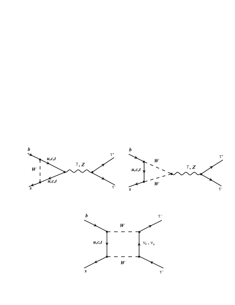
Figure 1: Feynman diagrams for $b\rightarrow s\tau^{+}\tau^{-}$ in the SM

In this work, we study the radiative $B\rightarrow\tau^{+}\tau^{-}\gamma$ decay in the general two-Higgs doublet model (2HDM). It is induced by the pure-leptonic decay $B\rightarrow\tau^{+}\tau^{-}$ and in principle, the latter can be used to determine the decay constant $f_{B}$ [2], as well as the fundamental parameters of the SM. However, it is well known that processes $B\rightarrow\ell^{+}\ell^{-}$ are helicity suppressed for light lepton modes, having branching ratios of the order of $10^{-9}$ for $\ell=\mu$ and $10^{-10}$ for $\ell=e$ channels [3]. Although the $B\rightarrow\tau^{+}\tau^{-}$ channel is free from this suppression, its observation is difficult due to low efficiency. If a photon line is attached to any of the charged lines (see Fig.1), the pure leptonic processes $B\rightarrow\ell^{+}\ell^{-}$ change into the corresponding radiative ones, $B\rightarrow\ell^{+}\ell^{-}\gamma$, so helicity suppression is overcome and larger branching ratios are expected. Depending on whether the photon is released from the initial quark or final lepton lines, there exist two different types of contributions, namely the so-called ”the structure dependent” (SD) and the ”internal Bremsstrahlung” (IB) respectively, while contributions coming from the release of the free photon from any charged internal line will be suppressed by a factor of $m^{2}_{b}/M^{2}_{W}$. The SD contribution is governed by the vector and axial vector form factors and it is free from the helicity suppression. Therefore, it could enhance the decay rates of the radiative processes $B\rightarrow\tau^{+}\tau^{-}\gamma$ in comparison to the decay rates of the pure leptonic ones $B\rightarrow\tau^{+}\tau^{-}$. As for the IB part of the contribution, it is proportional to the ratio $m_{\ell}/m_{B}$ and therefore it is still helicity suppressed for the light charged lepton modes while it enhances the amplitude considerably for $\ell=\tau$ mode. Indeed, $B\rightarrow\ell^{+}\ell^{-}\gamma$ decay have been investigated in the framework of the SM for light and heavy lepton modes [3]-[5], as well as in the models beyond the SM [6, 7], and it was found that in the SM $BR(B\rightarrow\ell^{+}\ell^{-}\gamma)=2.35\times 10^{-9}\cite[cite]{[\@@bibref{}{Eilam1}{}{}]},1.90\times 10^{-9}\cite[cite]{[\@@bibref{}{Aliev1}{}{}]},9.54\times 10^{-9}$ [5], for $\ell=e,\mu,\tau$, respectively. With long distance contributions, $BR(B\rightarrow\tau^{+}\tau^{-}\gamma)=1.52\times 10^{-8}$ was obtained [5]. In 2HDM, in contrast to the channels with light leptons, the channel $B\rightarrow\tau^{+}\tau^{-}\gamma$ receives additional contributions from the neutral Higgs boson (NHB) exchanges, in addition to SD and IB ones. In [6], $B\rightarrow\tau^{+}\tau^{-}\gamma$ decay is investigated in model I and II types of the 2HDM including NHB effects and shown that these effects are sizable when $\tan\beta$ is large. Our aim in this work is to study the sensitivity of the physically measurable quantities, such as branching ratio, photon energy density, forward-backward asymmetry of the final lepton and lepton polarization asymmetry, to the NHB effects, as well as to the model III parameters, like the Yukawa couplings $\bar{\xi}^{D}_{N,bb}$ and $\bar{\xi}^{D}_{N,\tau\tau}$.

The work is organized as follows. In section 2, after a brief summary about the main points of the general 2HDM, we first present the leading order (LO) QCD corrected effective Hamiltonian for the process $b\rightarrow s\tau^{+}\tau^{-}$, including the NHB effects and then give the matrix element for the exclusive $B\rightarrow\tau^{+}\tau^{-}\gamma$ decay, together with the explicit expressions for the double differential decay width, photon energy distribution, forward-backward asymmetry and the polarization asymmetry of the final lepton $\tau^{-}$. Section 3 is devoted to the numerical analysis of the dependencies of these observables on the model III parameters and also on NHB effects. Finally, in the Appendix, we give the explicit forms of the operators appearing in the Hamiltonian and the corresponding Wilson coefficients.

2 The $B\rightarrow\tau^{+}\tau^{-}\gamma$ decay in the framework of the general 2HDM

The 2HDM is the minimal extension of the SM, which consists of adding a second doublet to the Higgs sector. In this model, there are one charged Higgs scalar, two neutral Higgs scalars and one neutral Higgs pseudoscalar. The general Yukawa Lagrangian, which is responsible for the interactions of quarks with gauge bosons, can be written as

$${\cal{L}}_{Y} = \eta^{U}_{ij}\bar{Q}_{iL}\tilde{\phi_{1}}U_{jR}+\eta^{D}_{ij}\bar{Q}_{iL}\phi_{1}D_{jR}+\xi^{U\,\dagger}_{ij}\bar{Q}_{iL}\tilde{\phi_{2}}U_{jR}+\xi^{D}_{ij}\bar{Q}_{iL}\phi_{2}D_{jR}+h.c.\,\,\,,$$ (1)

where $i,j$ are family indices of quarks , $L$ and $R$ denote chiral projections $L(R)=1/2(1\mp\gamma_{5})$, $\phi_{m}$ for $m=1,2$, are the two scalar doublets, $Q_{iL}$ are quark doublets, $U_{jR}$, $D_{jR}$ are the corresponding quark singlets, $\eta^{U,D}_{ij}$ and $\xi^{U,D}_{ij}$ are the matrices of the Yukawa couplings. The Yukawa Lagrangian in Eq. (1) opens up the possibility that there appear tree-level FCNC. In the SM and in model I and model II types of the 2HDM, such FCNC at tree level are forbidden by the GIM mechanism [8] and by an ad hoc discrete symmetry [9], respectively. However, tree-level FCNC are permitted in the general 2HDM, and this type of 2HDM is referred to as model III in the literature.

In this model, it is possible to choose $\phi_{1}$ and $\phi_{2}$ in the following form

$$\phi_{1}=\frac{1}{\sqrt{2}}\left[\left(\begin{array}[]{c c}0\\ v+H^{0}\end{array}\right)\;+\left(\begin{array}[]{c c}\sqrt{2}\chi^{+}\\ i\chi^{0}\end{array}\right)\right]\,;\phi_{2}=\frac{1}{\sqrt{2}}\left(\begin{array}[]{c c}\sqrt{2}H^{+}\\ H_{1}+iH_{2}\end{array}\right)\,\,$$ (8)

with the vacuum expectation values,

$$<\phi_{1}>=\frac{1}{\sqrt{2}}\left(\begin{array}[]{c c}0\\ v\end{array}\right)\,\,;<\phi_{2}>=0\,\,.$$ (11)

With this choice, the SM particles can be collected in the first doublet and the new particles in the second one. Further, we take $H_{1}$, $H_{2}$ as the mass eigenstates $h^{0}$, $A^{0}$ respectively. Note that, at tree level, there is no mixing among CP even neutral Higgs bosons, namely the SM one, $H^{0}$, and beyond, $h^{0}$.

The part which produces FCNC at tree level is

$${\cal{L}}_{Y,FC}=\xi^{U\,\dagger}_{ij}\bar{Q}_{iL}\tilde{\phi_{2}}U_{jR}+\xi^{D}_{ij}\bar{Q}_{iL}\phi_{2}D_{jR}+\xi^{D}_{kl}\bar{l}_{kL}\phi_{2}E_{lR}+h.c.\,\,.$$ (12)

In Eq.(12), the couplings $\xi^{U,D}$ for the flavor-changing charged interactions are

$$\xi^{U}_{ch} = \xi_{neutral}\,\,V_{CKM}\,\,,$$

$$\xi^{D}_{ch} = V_{CKM}\,\,\xi_{neutral}\,\,,$$ (13)

where $\xi^{U,D}_{neutral}$ is defined by the expression

$$\xi^{U(D)}_{N}=(V_{R(L)}^{U(D)})^{-1}\xi^{U,(D)}V_{L(R)}^{U(D)}\,,$$ (14)

and $\xi^{U,D}_{neutral}$ is denoted as $\xi^{U,D}_{N}$. Here the charged couplings are the linear combinations of neutral couplings multiplied by $V_{CKM}$ matrix elements (see [10] for details).

After this brief summary about the general 2HDM, now we would like to present the calculation of the matrix element for the $B\rightarrow\tau^{+}\tau^{-}\gamma$ decay . For a general investigation of the $B\rightarrow\tau^{+}\tau^{-}\gamma$ decay, we start with the LO QCD corrected effective Hamiltonian which induces the corresponding quark level process $b\rightarrow s\,\tau^{+}\tau^{-}$, given by [11]

$${\cal H}=\frac{-4\,G_{F}}{\sqrt{2}}V_{tb}V_{ts}^{*}\Bigg{\{}\sum_{i=1}^{10}C_{i}(\mu)O_{i}(\mu)+\sum_{i=1}^{10}C_{Q_{i}}(\mu)Q_{i}(\mu)\Bigg{\}}\,,$$ (15)

where $O_{i}$ are current-current $(i=1,2)$, penguin $(i=1,..,6)$, magnetic penguin $(i=7,8)$ and semileptonic $(i=9,10)$ operators . The additional operators $Q_{i},(i=1,..,10)$ are due to the NHB exchange diagrams, which give considerable contributions in the case that the lepton pair is $\tau^{+}\tau^{-}$ [11]. $C_{i}(\mu)$ and $C_{Q_{i}}(\mu)$ are Wilson coefficients renormalized at the scale $\mu$. All these operators and the Wilson coefficients, together with their initial values calculated at $\mu=m_{W}$ in the SM and also the additional coefficients coming from the new Higgs scalars are presented in Appendix A.

The short distance contributions for $B\rightarrow\tau^{+}\tau^{-}\gamma$ decay come from the box, Z and photon penguin diagrams, which are obtained from the diagrams of Fig. (1) by attaching an additional photon line either to the initial quark lines that contribute to the SD part of the amplitude, or to the final lepton lines, which give the so-called IB part of the amplitude. Following this framework, the general form of the gauge invariant amplitude corresponding to Fig.(1) can be written as the sum of the SD and IB parts

$${\cal M}(B\rightarrow\tau^{+}\tau^{-}\gamma) = {\cal M}_{SD}+{\cal M}_{IB}\,,$$ (16)

where

$${\cal M}_{SD} = \frac{\alpha G_{F}}{2\sqrt{2}\,\pi}V_{tb}V_{ts}^{*}\frac{e}{m_{B}^{2}}\,\Bigg{\{}\bar{\tau}\gamma^{\mu}\tau\,\Big{[}A_{1}\epsilon_{\mu\nu\alpha\beta}\varepsilon^{\ast\nu}q^{\alpha}k^{\beta}+i\,A_{2}\Big{(}\varepsilon_{\mu}^{\ast}(kq)-(\varepsilon^{\ast}q)k_{\mu}\Big{)}\Big{]}$$ (17)

$$+ \bar{\tau}\gamma^{\mu}\gamma_{5}\tau\,\Big{[}B_{1}\epsilon_{\mu\nu\alpha\beta}\varepsilon^{\ast\nu}q^{\alpha}k^{\beta}+i\,B_{2}\Big{(}\varepsilon_{\mu}^{\ast}(kq)-(\varepsilon^{\ast}q)k_{\mu}\Big{)}\Big{]}\Bigg{\}}\,,$$

and

$${\cal M}_{IB} = \frac{\alpha G_{F}}{2\sqrt{2}\,\pi}V_{tb}V_{ts}^{*}ef_{B}i\,\Bigg{\{}F\,\bar{\tau}\Bigg{(}\frac{{\not\!\varepsilon}^{\ast}{\not\!p}_{B}}{2p_{1}k}-\frac{{\not\!p}_{B}{\not\!\varepsilon}^{\ast}}{2p_{2}k}\Bigg{)}\gamma_{5}\tau$$ (18)

$$+ F_{1}\,\bar{\tau}\Bigg{[}\frac{{\not\!\varepsilon}^{\ast}{\not\!p}_{B}}{2p_{1}k}-\frac{{\not\!p}_{B}{\not\!\varepsilon}^{\ast}}{2p_{2}k}+2m_{\tau}\Bigg{(}\frac{1}{2p_{1}k}+\frac{1}{2p_{2}k}\Bigg{)}{\not\!\varepsilon}^{\ast}\Bigg{]}\tau\Bigg{\}}~{},$$

where

$$A_{1} = \frac{-2}{q^{2}}m_{b}C^{eff}_{7}g_{1}+C^{eff}_{9}g~{},$$

$$A_{2} = \frac{-2}{q^{2}}m_{b}C^{eff}_{7}f_{1}+C^{eff}_{9}f~{},$$

$$B_{1} = C_{10}\,g~{},$$ (19)

$$B_{2} = C_{10}\,f~{},$$

$$F = 2m_{\tau}C_{10}+\frac{m^{2}_{B}}{m^{2}_{b}}C_{Q_{2}}~{},$$

$$F_{1} = \frac{m^{2}_{B}}{m^{2}_{b}}C_{Q_{1}}~{}.$$ (20)

In Eqs. (17) and (18), $\varepsilon_{\mu}^{\ast}$ and $k_{\mu}$ are the four vector polarization and four momentum of the photon, respectively, $q$ is the momentum transfer and $p_{B}$ is the momentum of the $B$ meson. The form factors $g$, $f$, $g_{1}$, $f_{1}$and $f_{B}$ are defined as follows [4, 12]:

$$\langle\gamma(k)\left|\bar{s}\gamma_{\mu}(1\mp\gamma_{5})b\right|B(p_{B})\rangle = \frac{e}{m_{B}^{2}}\Big{\{}\epsilon_{\mu\nu\lambda\sigma}\varepsilon^{\ast\nu}q^{\lambda}k^{\sigma}g(q^{2})\pm i\,\Big{[}\varepsilon^{\ast\mu}(kq)-(\varepsilon^{\ast}q)k^{\mu}\Big{]}f(q^{2})\Big{\}}~{},$$

$$\langle\gamma|\bar{s}i\sigma_{\mu\nu}k_{\nu}(1\mp\gamma_{5})b|B\rangle = \frac{e}{m_{B}^{2}}\Bigg{\{}\epsilon_{\mu\alpha\beta\sigma}\epsilon_{\alpha}^{*}k_{\beta}q_{\sigma}\,g_{1}(p^{2})\mp~{}i\left[\epsilon_{\mu}^{*}(kq)-(\epsilon^{*}k)q_{\mu}\right]\,f_{1}(p^{2})\Bigg{\}}~{},$$ (21)

$$\langle 0|\bar{s}\gamma_{\mu}\gamma_{5}b|B\rangle = -~{}if_{B}p_{B\mu}~{}.$$

In obtaining the expressions (17) and (18), we have also used

$$\langle 0|\bar{s}\sigma_{\mu\nu}(1+\gamma_{5})b|B\rangle = 0~{},$$

and conservation of the vector current. Note that in contrast to ${\cal M}_{SD}$ part of the amplitude, its ${\cal M}_{IB}$ part receives contributions from NHB exchange diagrams, which are represented by the factors $F$ and $F_{1}$ in Eq. (18). During the calculations of these NHB contributions in model III, we encountered logarithmic divergences and used the on-shell renormalization scheme to overcome them. (For details, see [13]).

We now examine the probability of the process $B\rightarrow\tau^{+}\tau^{-}\gamma$ as a function of the four momenta of the particles. In the center of mass (CM) frame of the dileptons $\tau^{+}\tau^{-}$, where we take $z=\cos\theta$ and $\theta$ is the angle between the momentum of the $B$-meson and that of $\tau^{-}$, double differential decay width is found to be

$$\frac{d\Gamma}{dx\,dz}=\frac{1}{(2\pi)^{3}64}\,x\,v\,m_{B}\,\left|{\cal M}\right|^{2}~{},$$ (22)

with

$$\left|{\cal M}\right|^{2} = \left|{\cal M}_{SD}\right|^{2}+\left|{\cal M}_{IB}\right|^{2}+2Re({\cal M}_{SD}{\cal M}^{*}_{IB})$$ (23)

where $x=2E_{\gamma}/m_{B}$ is the dimensionless photon energy and $v=\sqrt{1-\frac{4r}{1-x}}$ with $r=m^{2}_{\tau}/m^{2}_{B}$. After some calculation, we get for the different parts of the squared matrix elements in Eq. (23) :

$$\left|{\cal M}_{SD}\right|^{2} = \left|\frac{\alpha G_{F}}{2\sqrt{2}\,\pi}V_{tb}V_{ts}^{*}\frac{e}{m^{2}_{B}}\right|^{2}\,\Bigg{(}8\,{\rm Re}\left(A^{*}_{2}B_{1}+A^{*}_{1}B_{2}\right)p_{B}^{2}\left(p_{1}q-p_{2}q\right)\left(p_{1}q+p_{2}q\right)~{}$$

$$+~{}4\left[\left|B_{1}\right|^{2}+\left|B_{2}\right|^{2}\right]\left[\left(p_{B}^{2}-2m_{\tau}^{2}\right)\left(\left(p_{1}q\right)^{2}+\left(p_{2}q\right)^{2}\right)-4m_{\tau}^{2}\left(p_{1}q\right)\left(p_{2}q\right)\right]~{}$$

$$+~{}4\left[\left|A_{1}\right|^{2}+\left|A_{2}\right|^{2}\right]\Big{[}\left(p_{B}^{2}+2m_{\tau}^{2}\right)\left(\left(p_{1}q\right)^{2}+\left(p_{2}q\right)^{2}\right)+~{}4m_{\tau}^{2}\left(p_{1}q\right)\left(p_{2}q\right)\Big{]}\Bigg{)}~{},$$

$$2\,{\rm Re}\left({\cal M}_{SD}{\cal M}_{IB}^{*}\right) = ~{}\left|\frac{\alpha G_{F}}{2\sqrt{2}\,\pi}V_{tb}V_{ts}^{*}\frac{e}{m_{B}}\right|^{2}\,f_{B}\Bigg{\{}16\,m_{\tau}\Bigg{[}{\rm Re}(A_{1}F^{*})\,\frac{\left(p_{1}q+p_{2}q\right)^{3}}{\left(p_{1}q\right)\left(p_{2}q\right)}~{}$$ (25)

$$+~{}{\rm Re}(B_{2}F^{*})\,\frac{\left(p_{1}q+p_{2}q\right)^{2}\left(p_{1}q-p_{2}q\right)}{\left(p_{1}q\right)\left(p_{2}q\right)}\Bigg{]}$$

$$-~{}\Bigg{[}{\rm Re}(A_{2}F^{*}_{1})\,\frac{\left(p_{1}q+p_{2}q\right)^{3}}{\left(p_{1}q\right)\left(p_{2}q\right)}-{\rm Re}(B_{1}F^{*}_{1})\,\frac{\left(p_{1}q+p_{2}q\right)^{2}\left(p_{1}q-p_{2}q\right)}{\left(p_{1}q\right)\left(p_{2}q\right)}\Bigg{]}$$

$$+~{}\frac{m_{B}^{2}}{m_{b}}{\rm Re}(A_{2}F^{*}_{1})\Big{[}\frac{(m_{\tau}^{2}-3p_{2}q)(p_{1}q)}{p_{2}q}+\frac{(2m_{\tau}^{2}-p_{B}^{2})(p_{2}q)}{p_{1}q}\Big{]}\Big{\}}~{},$$

$$\left|{\cal M}_{IB}\right|^{2}=-~{}\left|\frac{\alpha G_{F}}{2\sqrt{2}\,\pi}V_{tb}V_{ts}^{*}ef_{B}\right|^{2}$$

$$\Bigg{\{}4(\left|F\right|^{2}+\left|F_{1}\right|^{2})\Bigg{[}\frac{1}{p_{1}q}\left(3m_{\tau}^{2}-p_{B}^{2}-2p_{2}q\right)+\frac{1}{p_{2}q}\left(3m_{\tau}^{2}-p_{B}^{2}-2p_{1}q\right)-4\Bigg{]}$$

$$+ \frac{2m_{\tau}^{2}}{\left(p_{1}q\right)^{2}}\Bigg{[}\left|F\right|^{2}\left(p_{B}^{2}+2p_{2}q\right)+\left|F_{1}\right|^{2}\left(p_{B}^{2}+2p_{2}q-4m_{\tau}^{2}\right)\Bigg{]}$$

$$+~{}\frac{2m_{\tau}^{2}}{\left(p_{2}q\right)^{2}}\Bigg{[}\ \left|F\right|^{2}\left(p_{B}^{2}+2p_{1}q\right)+\left|F_{1}\right|^{2}\left(p_{B}^{2}+2p_{1}q-4m_{\tau}^{2}\right)\Bigg{]}~{}$$

$$+\frac{2}{\left(p_{1}q\right)\left(p_{2}q\right)}\Bigg{[}\left|F\right|^{2}p_{B}^{2}\left(2m_{\tau}^{2}-p_{B}^{2}\right)-\left|F_{1}\right|^{2}\left(p_{B}^{2}+2p_{2}q-4m_{\tau}^{2}\right)\Bigg{]}\Bigg{\}}~{}.$$

There is a singularity in $\left|{\cal M}_{IB}\right|^{2}$ at the lower limit of the photon energy due to the soft photon emission from charged lepton line, while $\left|{\cal M}_{SD}\right|^{2}$ and $Re({\cal M}_{SD}{\cal M}^{*}_{IB})$ terms are free from this singularity. It has been shown that when processes $B\rightarrow\tau^{+}\tau^{-}\gamma$ and $B\rightarrow\tau^{+}\tau^{-}$ are considered together, the singular terms in $\left|{\cal M}_{IB}\right|^{2}$ exactly cancel the ${\cal O}(\alpha)$ virtual correction in $B\rightarrow\tau^{+}\tau^{-}$ amplitude. But instead of this approach we prefer the one used in ref.[5] which amounts to impose a cut on the photon energy, i.e., we require $E_{\gamma}\geq 50\,$ MeV. This restriction means that we only consider the hard photons in the process $B\rightarrow\tau^{+}\tau^{-}\gamma$. Therefore, the Dalitz boundary for the dimensionless photon energy is taken as

$$\delta\leq x\leq 1-\frac{4m_{\tau}^{2}}{m^{2}_{B}}~{},$$ (27)

with $\delta=0.01$.

Using Eqs. (22)-(2), we get the following result for the double differential decay width

$$\frac{d\Gamma}{dxdz} = \left|\frac{\alpha G_{F}}{2\sqrt{2}\,\pi}V_{tb}V_{ts}^{*}\right|^{2}\,\frac{\alpha}{\left(2\,\pi\right)^{3}}\,\frac{\pi}{4}\,m_{B}\,x\,v\,$$

$$\Bigg{\{}\frac{m^{2}_{B}}{32}\,x^{2}\,\Bigg{[}((1+z^{2})(1-x-4r))(\left|A_{1}\right|^{2}+\left|A_{2}\right|^{2}+\left|B_{1}\right|^{2}+\left|B_{2}\right|^{2})+8r(\left|A_{1}\right|^{2}+\left|A_{2}\right|^{2})$$

$$+ 4z\sqrt{(1-x)(1-x-4r)}\mbox{\rm Re}(A_{2}B^{*}_{1}+A_{1}B^{*}_{2})\Bigg{]}$$

$$+ f_{B}m_{\tau}\frac{(x-1)}{((z^{2}-1)(x-1)+4rz^{2})}\Bigg{[}vxz\mbox{\rm Re}(B_{2}F^{*}-B_{1}F^{*}_{1})+(1-4r-z^{2}(1-x-4r))$$

$$\mbox{\rm Re}(A_{2}F^{*}_{1})-x\mbox{\rm Re}(A_{1}F^{*})\Bigg{]}+f^{2}_{B}\frac{(1-x)}{x^{2}((z^{2}-1)(x-1)+4rz^{2})^{2}}$$

$$\Bigg{[}\left|F\right|^{2}\left((-2+4x-3x^{2}+x^{3}+8r(1-x))(z^{2}-1)+4rx^{2}z^{2}\right)$$

$$+ \left|F_{1}\right|^{2}\left(\left(32r^{2}(x-1)+4r(4-6x+2x^{2})-2+4x-3x^{2}+x^{3}\right)(z^{2}-1)+x^{2}z^{2}\right)\Bigg{]}\Bigg{\}}\,.$$

Integrating the angle variable, we find the photon energy distribution given by

$$\frac{d\Gamma}{dx} = \left|\frac{\alpha G_{F}}{2\sqrt{2}\,\pi}V_{tb}V_{ts}^{*}\right|^{2}\,\frac{\alpha}{\left(2\,\pi\right)^{3}}\,\frac{\pi}{4}\,m_{B}\,D(x)$$ (29)

where

$$D(x) = \frac{m_{B}^{2}}{12}x^{3}v\,\Bigg{[}(\left|A_{1}\right|^{2}+\left|A_{2}\right|^{2})(1+2r-x)+(\left|B_{1}\right|^{2}+\left|B_{2}\right|^{2})(1-4r-x)\Bigg{]}$$ (30)

$$- f_{B}m_{\tau}\,x\,\Bigg{[}2v(1-x)\mbox{\rm Re}(A_{2}F^{*}_{1})+{\rm ln}\frac{1+v}{1-v}\Bigg{(}(x-4r)\mbox{\rm Re}(A_{2}F^{*}_{1})-x\mbox{\rm Re}(A_{1}F^{*})\Bigg{)}\Bigg{]}$$

$$- 2f^{2}_{B}\Bigg{[}v\frac{(1-x)}{x}\Bigg{(}\left|F\right|^{2}+(1-4r)\left|F_{1}\right|^{2}\Bigg{)}+\,{\rm ln}\frac{1+v}{1-v}\Bigg{(}\Bigg{(}1+\frac{2r}{x}-\frac{1}{x}-\frac{x}{2}\Bigg{)}\left|F\right|^{2}$$

$$+ \Bigg{(}(1-4r)-\frac{2\left(1-6r+8r^{2}\right)}{x}-\frac{x}{2}\Bigg{)}\left|F_{1}\right|^{2}\Bigg{)}\Bigg{]}~{}.$$

We also give the forward-backward asymmetry, $A_{FB}$, in $B\rightarrow\tau^{+}\tau^{-}\gamma$. Using the definition of differential $A_{FB}$

$$A_{FB}(x) = \frac{\int^{1}_{0}dz\frac{d\Gamma}{dz}-\int^{0}_{-1}dz\frac{d\Gamma}{dz}}{\int^{1}_{0}dz\frac{d\Gamma}{dz}+\int^{0}_{-1}dz\frac{d\Gamma}{dz}}$$ (31)

we find

$$A_{FB}=\frac{\int\,dx\,E(x)}{\int\,dx\,D(x)}\,,$$ (32)

where

$$E(x) = -4\,v\,x^{2}\Bigg{(}m^{2}_{B}\,x\,\sqrt{(x-1)(x-1+4r)}\mbox{\rm Re}(A_{1}A^{*}_{2}-B_{1}B^{*}_{2})$$

$$+ 4f_{B}m_{\tau}\,v\,\Bigg{(}\frac{x-1}{x-1+4r}\Bigg{)}\ln\frac{4r}{x-1}\mbox{\rm Re}((A_{2}-B_{2})F^{*}-(A_{1}-B_{1})F^{*}_{1})\Bigg{)}$$

and $D(x)$ is given by Eq.(30).

Finally, we would like to discuss the $\tau^{-}$ lepton polarization effects for the process $B\rightarrow\tau^{+}\tau^{-}\gamma$. The longitudinal polarization asymmetry of the $\tau^{-}$ lepton is defined as

$$P_{L}(x) = \frac{(d\Gamma(S_{L})/dx)-(d\Gamma(-S_{L})/dx)}{(d\Gamma(S_{L})/dx)+(d\Gamma(-S_{L})/dx)}$$ (34)

where $S_{L}$ is the orthogonal unit vector for the polarization of the $\tau^{-}$ lepton to the longitudinal direction (L) and in the CM frame of the $\tau^{+}\tau^{-}$ system, it is defined as

$$S^{\mu}_{L} = \Bigg{(}\frac{|\vec{p}_{1}|}{m_{\tau}}\,,\,\frac{E_{\tau}\vec{p}_{1}}{m_{\tau}|\vec{p}_{1}|}\,\Bigg{)}.$$ (35)

Here, $\vec{p}_{1}$ and $E_{\tau}$ are the three momentum and energy of the $\tau^{-}$ lepton in the CM frame, respectively. Calculation of $P_{L}$ leads to the following result

$$P_{L} = \frac{2}{3}\frac{1}{vD(x)}\Bigg{\{}-m^{2}_{B}v^{3}x^{2}(-1+x)^{2}(\left|A_{1}\right|^{2}+\left|A_{2}\right|^{2}-\left|B_{1}\right|^{2}-\left|B_{2}\right|^{2})$$ (36)

$$+ 12f^{2}_{B}\frac{1}{(-1+x)^{2}}(1+x^{2}-4r(1+x))\Bigg{(}xv+(2r-x){\rm ln}\frac{1+v}{1-v}\Bigg{)}\,\mbox{\rm Re}(FF^{*}_{1})$$

$$+ 6f_{B}m_{\tau}\Bigg{[}\Bigg{(}vx-2r{\rm ln}\frac{1+v}{1-v}\Bigg{)}((1+x)\,\mbox{\rm Re}((A_{2}+B_{2})F^{*})+(-1+x)\,\mbox{\rm Re}((A_{1}+B_{1})F^{*}_{1}))$$

$$+ (-1+x)\Bigg{(}xv+(2r-x){\rm ln}\frac{1+v}{1-v}\Bigg{)}\,\mbox{\rm Re}((A_{2}-B_{2})F^{*}_{1}-(A_{1}-B_{1})F^{*})\Bigg{]}\Bigg{\}}$$

In order to investigate the dependence of the $\tau^{-}$ lepton polarization on the model III parameters, we eliminate the other parameter, namely $x$, by performing the $x$-integrations over the allowed kinematical region (Eq.(27)) so as to obtain the averaged lepton polarization. For the longitudinal component the averaged lepton polarization is defined as

$$<P_{L}> = \frac{\int_{\delta}^{(1-4m^{2}_{\tau}/m^{2}_{B})}P_{L}\,\frac{d\Gamma}{dx}\,dx}{\int_{\delta}^{(1-4m^{2}_{\tau}/m^{2}_{B})}\frac{d\Gamma}{dx}\,dx}.$$

For the process $B\rightarrow\tau^{+}\tau^{-}\gamma$, the lepton polarization has, in addition to the longitudinal component $P_{L}$, transverse and normal components. Since these two orthogonal components are proportional to the tau lepton mass, they are expected to be significant for the $\tau^{+}\tau^{-}$ channel. We shall discuss their effects in a more detailed paper.

3 Numerical analysis and discussion

To calculate the decay width, first of all, we need the explicit forms of the form factors $g,~{}f,~{}g_{1}$ and $f_{1}$. In refs. [2] and [12], they are calculated in the framework of light–cone QCD sum rules and their $q^{2}$ dependences, to a very good accuracy, can be represented in the following dipole forms,

$$g(q^{2}) = \frac{g(0)}{\left(1-\frac{q^{2}}{m_{g}^{2}}\right)^{2}~{}},~{}~{}~{}~{}~{}~{}~{}~{}~{}~{}f(q^{2})=\frac{f(0)}{\left(1-\frac{q^{2}}{m_{f}^{2}}\right)^{2}}~{},$$

$$g_{1}(q^{2}) = \frac{g_{1}(0)}{\left(1-\frac{q^{2}}{m^{2}_{g_{1}}}\right)^{2}}~{},~{}~{}~{}~{}~{}~{}~{}~{}~{}f_{1}(q^{2})=\frac{f_{1}(0)}{\left(1-\frac{q^{2}}{m^{2}_{f_{1}}}\right)^{2}}~{},$$ (37)

where

$$g(0) = 1\,GeV\,,\,f(0)=0.8\,GeV\,,\,g_{1}(0)=3.74\,GeV^{2}\,,\,f_{1}(0)=0.68\,GeV^{2}\,,$$

$$m_{g} = 5.6\,GeV\,,\,m_{f}=6.5\,GeV\,,\,m_{g_{1}}=6.4\,GeV\,,\,m_{f_{1}}=5.5\,GeV\,.$$

In addition to these form factors, the other input parameters which we have used in our numerical calculations are given in table I.

For the free parameters of the model III, namely, the masses of charged and neutral Higgs bosons, $m_{H^{\pm}},m_{A^{0}},m_{h^{0}},m_{H^{0}}$ and the Yukawa couplings ($\xi_{ij}^{U,D}$), we use the restrictions coming from $B\rightarrow X_{s}\,\gamma$ decay, whose BR is given by CLEO measurement [14] as

$$BR(B\rightarrow X_{s}\,\gamma) = (3.15\pm 0.35\pm 0.32)\times 10^{-4}$$ (38)

and $B^{0}-\bar{B}^{0}$ mixing [10], $\rho$ parameter [15] and neutron electric-dipole moment [16], that yields $\bar{\xi}^{D}_{N,ib}\sim 0$ and $\bar{\xi}^{D}_{N,ij}\sim 0$, where the indices $i,j$ denote d and s quarks, and $\bar{\xi}_{Ntc}<<\bar{\xi}^{U}_{Ntt}$. Therefore, we take into account only the Yukawa couplings of b and t quarks, $\bar{\xi}^{U}_{N,tt}$ and $\bar{\xi}^{D}_{N,bb}$ and also $\bar{\xi}^{D}_{N,\tau\tau}$. Further, in our numerical calculations we adopted the restriction, $0.257\leq|C_{7}^{eff}|\leq 0.439$ due to the CLEO measurement, Eq.(38), (see [10] for details) and the redefinition

$$\xi^{U,D}=\sqrt{\frac{4G_{F}}{\sqrt{2}}}\bar{\xi}^{U,D}\,\,.$$

Before we present our results, a small note about the calculations of the long distance (LD) effects is in place. We take into account five possible resonances for the LD effects coming from the reaction $b\rightarrow s\,\psi_{i}\rightarrow s\,\tau^{+}\tau^{-}$, where $i=1,...,5$ and divide the integration region into two parts: $\delta\leq x\leq 1-((m_{\psi_{2}}+0.02)/m_{B})^{2}$ and $1-((m_{\psi_{2}}-0.02)/m_{B})^{2}\leq x\leq 1-(2m_{\tau}/m_{B})^{2}$, where $m_{\psi_{2}}=3.686$ GeV is the mass of the second resonance. (See Appendix for the details of LD contributions).

In this section, we first study the dimensionless photon energy dependence of the differential branching ratio $(dBR/dx)$ and the model III parameters dependence of the BR and also the forward-backward asymmetry, $A_{FB}$. The results of our calculations are presented through the graphs in Fig.(2)-(11). In Fig.(2), we present $dBR(B\rightarrow\tau^{+}\tau^{-}\gamma)/dx$ as a function of $x=2E_{\gamma}/m_{B}$ for $\bar{\xi}_{N,bb}^{D}=40\,m_{b}$ and $\bar{\xi}_{N,\tau\tau}^{D}=10\,m_{\tau}$, in case of the ratio $|r_{tb}|\equiv|\frac{\bar{\xi}_{N,tt}^{U}}{\bar{\xi}_{N,bb}^{D}}|<1$, including the long distance contributions. Here, the differential BR lies in the region bounded by dashed (solid) curves for $C^{eff}_{7}<0$ ($C^{eff}_{7}>0$). We see from this figure that there is an enhancement for the $dBR(B\rightarrow\tau^{+}\tau^{-}\gamma)/dx$ in model III compared to the SM result for the $C^{eff}_{7}>0$ case, while for $C^{eff}_{7}<0$, model III predictions almost coincide with the SM one (small dashed curve). Fig. (3) is devoted the same dependence of differential BR, but for $\bar{\xi}_{N,bb}^{D}=0.1\,m_{b}$ and $\bar{\xi}_{N,\tau\tau}^{D}=m_{\tau}$, in case of the ratio $r_{tb}>1$. We see that model III predictions for the $C^{eff}_{7}>0$ and $C^{eff}_{7}<0$ almost coincide and they are one order larger compared to both $|r_{tb}|<1$ case and the SM one.

Fig (4) and (5) show $\bar{\xi}_{N,bb}^{D}/m_{b}$ dependence of BR for $\bar{\xi}_{N,\tau\tau}^{D}=m_{\tau}$ , in case of the ratio $|r_{tb}|<1$ and $r_{tb}>1$, respectively. In Fig.(4), BR is restricted in the region between dashed lines (solid curves) for $C^{eff}_{7}<0$ ($C^{eff}_{7}>0$), while the small dashed straight line shows the SM contribution. In Fig. (5), there is a single curve since the contributions for both $C^{eff}_{7}>0$ and $C^{eff}_{7}<0$ fit onto each other. We see that BR is quite sensitive to the parameter $\bar{\xi}_{N,bb}^{D}/m_{b}$, for both $|r_{tb}|<1$ and $r_{tb}>1$, however the behavior is opposite for these two cases; for $|r_{tb}|<1$, BR is decreasing with the increasing values of $\bar{\xi}_{N,bb}^{D}/m_{b}$, while for $r_{tb}>1$, it is increasing. Further, BR is 2-3 orders larger compared to the SM result for $r_{tb}>1$ case. For $|r_{tb}|<1$, the enhancement with respect to the SM prediction is relatively moderate; nearly $(30-40)\%$ for $C^{eff}_{7}>0$, but for $C^{eff}_{7}<0$ they almost coincide with the SM one.

The dependence of the BR on the Yukawa coupling $\bar{\xi}_{N,\tau\tau}^{D}$ is presented in Fig. (6) ((7)), for $|r_{tb}|<1$ ( $r_{tb}>1$) case with $\bar{\xi}_{N,bb}^{D}=40\,m_{b}$ ($\bar{\xi}_{N,bb}^{D}=0.1\,m_{b}$). It is seen that BR is increasing with the increasing values of $\bar{\xi}_{N,\tau\tau}^{D}$ and this is the contribution due to NHB effects. From Fig. (6), we see that the BR lies in the region bounded by solid lines for $C^{eff}_{7}>0$ and it is sensitive to the NHB effects, while for $C^{eff}_{7}<0$, it is almost the same as the SM result (dashed straight line). Note that the SM prediction for the BR is $7.89\times 10^{-9}$ and in model III without NHB effects, when $|r_{tb}|<1$ it is in between $(7.83-7.97)\times 10^{-9}$ for $C^{eff}_{7}>0$ and $(8.73-8.50)\times 10^{-9}$ for $C^{eff}_{7}<0$. When $r_{tb}>1$, upper and lower limits of the BR without NHB effects are $(1.03-1.04)\times 10^{-7}$ for both $C^{eff}_{7}>0$ and $C^{eff}_{7}<0$. Thus, contribution from NHB effects is seen to reach the values that are two orders of magnitude larger than the overall contributions for both $|r_{tb}|<1$ and $r_{tb}>1$, even for small values of $\bar{\xi}_{N,\tau\tau}^{D}$.

In Fig. (8), the differential $A_{FB}(x)$ is shown for $\bar{\xi}_{N,bb}^{D}=40\,m_{b}$ and $\bar{\xi}_{N,\tau\tau}^{D}=10\,m_{\tau}$, in case of the ratio $|r_{tb}|<1$. Here, $A_{FB}(x)$ is restricted in the region between solid curves for $C^{eff}_{7}>0$. It is seen that the value of $|A_{FB}(x)|$ stands less than the SM one. The dashed curves represent $C^{eff}_{7}<0$ case and they almost coincide with the SM prediction for $A_{FB}(x)$. Fig.(9) is the same as Fig. (8), but for $r_{tb}>1$ with $\bar{\xi}_{N,bb}^{D}=0.1\,m_{b}$ . For this case, the sign of $A_{FB}(x)$ is opposite to the SM prediction and $|A_{FB}(x)|$ is one order of magnitude smaller than the SM one.

In Fig. (10) we plot the $A_{FB}$ as a function of the Yukawa coupling $\bar{\xi}_{N,\tau\tau}^{D}$ for $\bar{\xi}_{N,bb}^{D}=40\,m_{b}$ and $|r_{tb}|<1$. $A_{FB}$ lies in the region bounded by dashed (solid) lines for $C^{eff}_{7}<0$ ( $C^{eff}_{7}>0$ ). As seen from Fig. (10) that $A_{FB}$ vanishes for the large values of $\bar{\xi}_{N,\tau\tau}^{D}$ for $C^{eff}_{7}>0$, while $C^{eff}_{7}<0$, it does not vanish in the given region of $\bar{\xi}_{N,\tau\tau}^{D}$. Contributions to $|A_{FB}|$ from model III stand less than the SM ones. Fig.(11) is the same as Fig. (10) , but for $r_{tb}>1$ with $\bar{\xi}_{N,bb}^{D}=0.1\,m_{b}$. Here, contributions for $C^{eff}_{7}>0$ and $C^{eff}_{7}<0$ coincide and both are restricted by the solid curves.

We present our analysis on the longitudinal component of the $\tau^{-}$ lepton polarization through the graphs in Figs.(12)-(15). The dependence of $P_{L}$ on $x$ is presented in Fig (12), for $|r_{tb}|<1$ case with $\bar{\xi}_{N,\tau\tau}^{D}=10\,m_{\tau}$. Here, $P_{L}$ is restricted in the region between dashed (solid ) curves for $C^{eff}_{7}<0$ ($C^{eff}_{7}>0$), while the small dashed curve shows the SM contribution. From this figure, we see that the 2HDM contributions change $P_{L}$ significantly compared to the SM case for $C^{eff}_{7}>0$, especially for the small values of $x$. Fig. (13) is the same as Fig. (12), but $r_{tb}>1$ with $\bar{\xi}_{N,bb}^{D}=0.1\,m_{b}$. In this figure, two solid curves restrict the possible values of $P_{L}$ for both $C^{eff}_{7}<0$ and $C^{eff}_{7}>0$ and it is seen that both the magnitude and the sign of $P_{L}$ are changed for $r_{tb}>1$.

The dependence of $<P_{L}>$ on the NHB parameter $\bar{\xi}_{N,\tau\tau}^{D}$ is presented in Fig. (14) ((15)), for $|r_{tb}|<1$ ( $r_{tb}>1$) case with $\bar{\xi}_{N,bb}^{D}=40\,m_{b}$ ($\bar{\xi}_{N,bb}^{D}=0.1\,m_{b}$). We see that for $|r_{tb}|<1$, $<P_{L}>$ lies in the region bounded by dashed lines (solid curves) for $C^{eff}_{7}<0$ ( $C^{eff}_{7}>0$) (Fig. (14)), while in case of $r_{tb}>1$, the contributions for both $C^{eff}_{7}<0$ and $C^{eff}_{7}>0$ coincide and they are represented by the single solid curve in Fig.(15). It is obvious that $<P_{L}>$ is very much sensitive to the NHB effects for both $|r_{tb}|<1$ and $r_{tb}>1$ cases. We note that SM prediction for $<P_{L}>$ is $-0.36$ and in model III without NHB effects, when $|r_{tb}|<1$, it is about $-0.31$ for $C^{eff}_{7}>0$ and $-0.36$ for $C^{eff}_{7}<0$. When $r_{tb}>1$, the value of $<P_{L}>$ without NHB effects is about $-0.36$ for both $C^{eff}_{7}>0$ and $C^{eff}_{7}<0$. Thus, the value of $<P_{L}>$ without NHB effects reaches at most the SM prediction, but NHB effects enhance it between $(5-100)\%$, even for small values of $\bar{\xi}_{N,\tau\tau}^{D}$.

Parameter	Value
$m_{\tau}$	$1.78$ (GeV)
$m_{c}$	$1.4$ (GeV)
$m_{b}$	$4.8$ (GeV)
$\alpha_{em}^{-1}$	129
$\lambda_{t}$	0.04
$m_{t}$	$175$ (GeV)
$m_{W}$	$80.26$ (GeV)
$m_{Z}$	$91.19$ (GeV)
$m_{H^{0}}$	$150$ (GeV)
$m_{h^{0}}$	$70$ (GeV)
$m_{A^{0}}$	$80$ (GeV)
$m_{H^{\pm}}$	$400$ (GeV)
$\Lambda_{QCD}$	$0.225$ (GeV)
$\alpha_{s}(m_{Z})$	$0.117$
$sin^{2}\theta_{W}$	$0.2325$

Table 1: The values of the input parameters used in the numerical calculations.

We would like to summarize our results:

• We observe an enhancement in the differential branching ratio and branching ratio for the exclusive process $B\rightarrow\tau^{+}\tau^{-}\gamma$ in the general 2HDM compared to the SM predictions. For $|r_{tb}|<1$ case, this enhancement is much more detectable for $C_{7}^{eff}>0$ case compared to the $C_{7}^{eff}<0$ one. For $r_{tb}>1$, we see that contributions for $C_{7}^{eff}>0$ and $C_{7}^{eff}<0$ almost coincide with each other, and the enhancement with respect to the SM is much more sizable.

• BR for $B\rightarrow\tau^{+}\tau^{-}\gamma$ decay is at the order of magnitude $10^{-9}$ ($10^{-7}$) in the SM and in model III without NHB effects for $|r_{tb}|<1$ ( $r_{tb}>1$). However, including NHB exchanges may enhance it almost two orders of magnitude compared to the SM prediction, even for the smaller values of $\bar{\xi}_{N,\tau\tau}^{D}$.

• $|A_{FB}|$ is at the order of magnitude $10^{-1}$ ($10^{-2}$) for $|r_{tb}|<1$ ($r_{tb}>1$) case and smaller compared to the SM results, which is -0.181.

• The 2HDM contributions change $P_{L}$ and $<P_{L}>$ greatly compared to the SM case and these quantities are very sensitive to the NHB effects.

In conclusion, we can say that experimental investigation of BR, $A_{FB}$ and $P_{L}$ may provide an essential test for the effects of NHB exchanges and new physics beyond the SM.

Appendix A The operator basis

The operator basis in the 2HDM (model III ) for our process is [11, 17, 18]

$$O_{1} = (\bar{s}_{L\alpha}\gamma_{\mu}c_{L\beta})(\bar{c}_{L\beta}\gamma^{\mu}b_{L\alpha}),$$

$$O_{2} = (\bar{s}_{L\alpha}\gamma_{\mu}c_{L\alpha})(\bar{c}_{L\beta}\gamma^{\mu}b_{L\beta}),$$

$$O_{3} = (\bar{s}_{L\alpha}\gamma_{\mu}b_{L\alpha})\sum_{q=u,d,s,c,b}(\bar{q}_{L\beta}\gamma^{\mu}q_{L\beta}),$$

$$O_{4} = (\bar{s}_{L\alpha}\gamma_{\mu}b_{L\beta})\sum_{q=u,d,s,c,b}(\bar{q}_{L\beta}\gamma^{\mu}q_{L\alpha}),$$

$$O_{5} = (\bar{s}_{L\alpha}\gamma_{\mu}b_{L\alpha})\sum_{q=u,d,s,c,b}(\bar{q}_{R\beta}\gamma^{\mu}q_{R\beta}),$$

$$O_{6} = (\bar{s}_{L\alpha}\gamma_{\mu}b_{L\beta})\sum_{q=u,d,s,c,b}(\bar{q}_{R\beta}\gamma^{\mu}q_{R\alpha}),$$

$$O_{7} = \frac{e}{16\pi^{2}}\bar{s}_{\alpha}\sigma_{\mu\nu}(m_{b}R+m_{s}L)b_{\alpha}{\cal{F}}^{\mu\nu},$$

$$O_{8} = \frac{g}{16\pi^{2}}\bar{s}_{\alpha}T_{\alpha\beta}^{a}\sigma_{\mu\nu}(m_{b}R+m_{s}L)b_{\beta}{\cal{G}}^{a\mu\nu}\,\,,$$

$$O_{9} = \frac{e}{16\pi^{2}}(\bar{s}_{L\alpha}\gamma_{\mu}b_{L\alpha})(\bar{\tau}\gamma^{\mu}\tau)\,\,,$$

$$O_{10} = \frac{e}{16\pi^{2}}(\bar{s}_{L\alpha}\gamma_{\mu}b_{L\alpha})(\bar{\tau}\gamma^{\mu}\gamma_{5}\tau)\,\,,$$

$$Q_{1} = \frac{e^{2}}{16\pi^{2}}(\bar{s}^{\alpha}_{L}\,b^{\alpha}_{R})\,(\bar{\tau}\tau)\,,$$

$$Q_{2} = \frac{e^{2}}{16\pi^{2}}(\bar{s}^{\alpha}_{L}\,b^{\alpha}_{R})\,(\bar{\tau}\gamma_{5}\tau)\,,$$

$$Q_{3} = \frac{g^{2}}{16\pi^{2}}(\bar{s}^{\alpha}_{L}\,b^{\alpha}_{R})\,\sum_{q=u,d,s,c,b}(\bar{q}^{\beta}_{L}\,q^{\beta}_{R})\,,$$

$$Q_{4} = \frac{g^{2}}{16\pi^{2}}(\bar{s}^{\alpha}_{L}\,b^{\alpha}_{R})\,\sum_{q=u,d,s,c,b}(\bar{q}^{\beta}_{R}\,q^{\beta}_{L})\,,$$

$$Q_{5} = \frac{g^{2}}{16\pi^{2}}(\bar{s}^{\alpha}_{L}\,b^{\beta}_{R})\,\sum_{q=u,d,s,c,b}(\bar{q}^{\beta}_{L}\,q^{\alpha}_{R})\,,$$

$$Q_{6} = \frac{g^{2}}{16\pi^{2}}(\bar{s}^{\alpha}_{L}\,b^{\beta}_{R})\,\sum_{q=u,d,s,c,b}(\bar{q}^{\beta}_{R}\,q^{\alpha}_{L})\,,$$

$$Q_{7} = \frac{g^{2}}{16\pi^{2}}(\bar{s}^{\alpha}_{L}\,\sigma^{\mu\nu}\,b^{\alpha}_{R})\,\sum_{q=u,d,s,c,b}(\bar{q}^{\beta}_{L}\,\sigma_{\mu\nu}q^{\beta}_{R})\,,$$

$$Q_{8} = \frac{g^{2}}{16\pi^{2}}(\bar{s}^{\alpha}_{L}\,\sigma^{\mu\nu}\,b^{\alpha}_{R})\,\sum_{q=u,d,s,c,b}(\bar{q}^{\beta}_{R}\,\sigma_{\mu\nu}q^{\beta}_{L})\,,$$

$$Q_{9} = \frac{g^{2}}{16\pi^{2}}(\bar{s}^{\alpha}_{L}\,\sigma^{\mu\nu}\,b^{\beta}_{R})\,\sum_{q=u,d,s,c,b}(\bar{q}^{\beta}_{L}\,\sigma_{\mu\nu}q^{\alpha}_{R})\,,$$

$$Q_{10} = \frac{g^{2}}{16\pi^{2}}(\bar{s}^{\alpha}_{L}\,\sigma^{\mu\nu}\,b^{\beta}_{R})\,\sum_{q=u,d,s,c,b}(\bar{q}^{\beta}_{R}\,\sigma_{\mu\nu}q^{\alpha}_{L})$$ (39)

where $\alpha$ and $\beta$ are $SU(3)$ colour indices and ${\cal{F}}^{\mu\nu}$ and ${\cal{G}}^{\mu\nu}$ are the field strength tensors of the electromagnetic and strong interactions, respectively. Note that there are also flipped chirality partners of these operators, which can be obtained by interchanging $L$ and $R$ in the basis given above in model III. However, we do not present them here since corresponding Wilson coefficients are negligible.

Appendix B The Initial values of the Wilson coefficients.

The initial values of the Wilson coefficients for the relevant process in the SM are [17]

$$C^{SM}_{1,3,\dots 6}(m_{W}) = 0\,\,,$$

$$C^{SM}_{2}(m_{W}) = 1\,\,,$$

$$C_{7}^{SM}(m_{W}) = \frac{3x_{t}^{3}-2x_{t}^{2}}{4(x_{t}-1)^{4}}\ln x_{t}+\frac{-8x_{t}^{3}-5x_{t}^{2}+7x_{t}}{24(x_{t}-1)^{3}}\,\,,$$

$$C_{8}^{SM}(m_{W}) = -\frac{3x_{t}^{2}}{4(x_{t}-1)^{4}}\ln x_{t}+\frac{-x_{t}^{3}+5x_{t}^{2}+2x_{t}}{8(x_{t}-1)^{3}}\,\,,$$

$$C_{9}^{SM}(m_{W}) = -\frac{1}{sin^{2}\theta_{W}}B(x_{t})+\frac{1-4\sin^{2}\theta_{W}}{\sin^{2}\theta_{W}}C(x_{t})-D(x_{t})+\frac{4}{9},\,\,,$$

$$C_{10}^{SM}(m_{W}) = \frac{1}{\sin^{2}\theta_{W}}(B(x_{t})-C(x_{t}))\,\,,$$

$$C_{Q_{i}}^{SM}(m_{W}) = 0~{}~{}~{}i=1,..,10$$ (40)

and for the additional part due to charged Higgs bosons are

$$C^{H}_{1,\dots 6}(m_{W}) = 0\,,$$

$$C_{7}^{H}(m_{W}) = Y^{2}\,F_{1}(y_{t})\,+\,XY\,F_{2}(y_{t})\,\,,$$

$$C_{8}^{H}(m_{W}) = Y^{2}\,G_{1}(y_{t})\,+\,XY\,G_{2}(y_{t})\,\,,$$

$$C_{9}^{H}(m_{W}) = Y^{2}\,H_{1}(y_{t})\,\,,$$

$$C_{10}^{H}(m_{W}) = Y^{2}\,L_{1}(y_{t})\,\,,$$ (41)

where

$$X = \frac{1}{m_{b}}~{}~{}~{}\left(\bar{\xi}^{D}_{N,bb}+\bar{\xi}^{D}_{N,sb}\frac{V_{ts}}{V_{tb}}\right)~{}~{},~{}~{}$$

$$Y = \frac{1}{m_{t}}~{}~{}~{}\left(\bar{\xi}^{U}_{N,tt}+\bar{\xi}^{U}_{N,tc}\frac{V^{*}_{cs}}{V^{*}_{ts}}\right)~{}~{}.~{}~{}$$ (42)

The NHB effects bring new operators and the corresponding Wilson coefficients read as

$$\!\!\!\!\!\!\!\!\!\!\!\!\!\!\!\!\!\!\!\!\!\!\!\!\!\!\!\!\!\!\!\!\!\!\!\!\!\!\!\!\!\!\!\!\!\!\!\!\!\!\!\!\!\!\!\!\!\!\!\!\!\!\!\!\!\!\!\!\!\!\!\!\!\!\!\!\!\!C^{A^{0}}_{Q_{2}}((\bar{\xi}^{U}_{N,tt})^{3})=\frac{\bar{\xi}^{D}_{N,\tau\tau}(\bar{\xi}^{U}_{N,tt})^{3}m_{b}y_{t}(\Theta_{5}(y_{t})z_{A}-\Theta_{1}(z_{A},y_{t}))}{32\pi^{2}m_{A^{0}}^{2}m_{t}\Theta_{1}(z_{A},y_{t})\Theta_{5}(y_{t})},$$

$$C^{A^{0}}_{Q_{2}}((\bar{\xi}^{U}_{N,tt})^{2})=\frac{\bar{\xi}^{D}_{N,\tau\tau}(\bar{\xi}^{U}_{N,tt})^{2}\bar{\xi}^{D}_{N,bb}}{32\pi^{2}m_{A^{0}}^{2}}\Big{(}\frac{(y_{t}(\Theta_{1}(z_{A},y_{t})-\Theta_{5}(y_{t})(xy+z_{A}))-2\Theta_{1}(z_{A},y_{t})\Theta_{5}(y_{t})\ln[\frac{z_{A}\Theta_{5}(y_{t})}{\Theta_{1}(z_{A},y_{t})}]}{\Theta_{1}(z_{A},y_{t})\Theta_{5}(y_{t})}\Big{)},$$

$$C^{A^{0}}_{Q_{2}}(\bar{\xi}^{U}_{N,tt}) = \frac{g^{2}\bar{\xi}^{D}_{N,\tau\tau}\bar{\xi}^{U}_{N,tt}m_{b}x_{t}}{64\pi^{2}m_{A^{0}}^{2}m_{t}}\Bigg{(}\frac{2}{\Theta_{5}(x_{t})}-\frac{xyx_{t}+2z_{A}}{\Theta_{1}(z_{A},x_{t})}-2\ln[\frac{z_{A}\Theta_{5}(x_{t})}{\Theta_{1}(z_{A},x_{t})}]$$

$$\!\!\!\!\!\!\!\!\!\!\!\!\!\!\!\!\!\!\!\!\!\!\!-xyx_{t}y_{t}(\frac{(x-1)x_{t}(y_{t}/z_{A}-1)-(1+x)y_{t})}{(\Theta_{6}-(x-y)(x_{t}-y_{t}))(\Theta_{3}(z_{A})+(x-y)(x_{t}-y_{t})z_{A})}-\frac{x(y_{t}+x_{t}(1-y_{t}/z_{A}))-2y_{t}}{\Theta_{6}\Theta_{3}(z_{A})})\Bigg{)}$$

$$\!\!\!C^{A^{0}}_{Q_{2}}(\bar{\xi}^{D}_{N,bb})=\frac{g^{2}\bar{\xi}^{D}_{N,\tau\tau}\bar{\xi}^{D}_{N,bb}}{64\pi^{2}m^{2}_{A^{0}}}\Big{(}1-\frac{x^{2}_{t}y_{t}+2y(x-1)x_{t}y_{t}-z_{A}(x^{2}_{t}+\Theta_{6})}{\Theta_{3}(z_{A})}+\frac{x^{2}_{t}(1-y_{t}/z_{A})}{\Theta_{6}}+2\ln[\frac{z_{A}\Theta_{6}}{\Theta_{2}(z_{A},x)}]\Big{)}$$

$$\!\!\!\!\!\!\!\!\!\!\!\!\!\!\!\!\!\!\!\!\!C^{H^{0}}_{Q_{1}}((\bar{\xi}^{U}_{N,tt})^{2})=\frac{g^{2}(\bar{\xi}^{U}_{N,tt})^{2}m_{b}m_{\tau}}{64\pi^{2}m^{2}_{H^{0}}m^{2}_{t}}\Bigg{(}\frac{x_{t}(1-2y)y_{t}}{\Theta_{5}(y_{t})}+\frac{(-1+2\cos^{2}\theta_{W})(-1+x+y)y_{t}}{\cos^{2}\theta_{W}\Theta_{4}(y_{t})}$$ (43)

$$+\frac{z_{H}(\Theta_{1}(z_{H},y_{t})xy_{t}+\cos^{2}\theta_{W}\,(-2x^{2}(-1+x_{t})yy^{2}_{t}+xx_{t}yy^{2}_{t}-\Theta_{8}z_{H}))}{\cos^{2}\theta_{W}\Theta_{1}(z_{H},y_{t})\Theta_{7}}\Bigg{)},$$

$$\!\!\!\!\!\!\!\!\!\!\!\!\!\!\!\!\!\!\!\!\!\!\!\!\!\!\!\!\!\!\!\!\!\!\!\!\!\!\!\!\!\!\!\!\!\!\!C^{H^{0}}_{Q_{1}}(\bar{\xi}^{U}_{N,tt})=\frac{g^{2}\bar{\xi}^{U}_{N,tt}\bar{\xi}^{D}_{N,bb}m_{\tau}}{64\pi^{2}m^{2}_{H^{0}}m_{t}}\Bigg{(}\frac{(-1+2\cos^{2}\theta_{W})\,y_{t}}{\cos^{2}\theta_{W}\,\Theta_{4}(y_{t})}-\frac{x_{t}y_{t}}{\Theta_{5}(y_{t})}+\frac{x_{t}y_{t}(xy-z_{H})}{\Theta_{1}(z_{H},y_{t})}$$

$$+\frac{(-1+2\cos^{2}\theta_{W})y_{t}z_{H}}{\cos^{2}\theta_{W}\Theta_{7}}-2x_{t}\,\ln\Bigg{[}\frac{\Theta_{5}(y_{t})z_{H}}{\Theta_{1}(z_{H},y_{t})}\Bigg{]}\Bigg{)},$$

$$C^{H^{0}}_{Q_{1}}(g^{4})=-\frac{g^{4}m_{b}m_{\tau}x_{t}}{128\pi^{2}m^{2}_{H^{0}}m^{2}_{t}}\Bigg{(}-1+\frac{(-1+2x)x_{t}}{\Theta_{5}(x_{t})+y(1-x_{t})}+\frac{2x_{t}(-1+(2+x_{t})y)}{\Theta_{5}(x_{t})}$$

$$-\frac{4\cos^{2}\theta_{W}(-1+x+y)+x_{t}(x+y)}{\cos^{2}\theta_{W}\Theta_{4}(x_{t})}+\frac{x_{t}(x(x_{t}(y-2z_{H})-4z_{H})+2z_{H})}{\Theta_{1}(z_{H},x_{t})}$$

$$+\frac{y_{t}((-1+x)x_{t}z_{H}+\cos^{2}\theta_{W}((3x-y)z_{H}+x_{t}(2y(x-1)-z_{H}(2-3x-y))))}{\cos^{2}\theta_{W}(\Theta_{3}(z_{H})+x(x_{t}-y_{t})z_{H})}$$

$$+2\,(x_{t}\ln\Bigg{[}\frac{\Theta_{5}(x_{t})z_{H}}{\Theta_{1}(z_{H},x_{t})}\Bigg{]}+\ln\Bigg{[}\frac{x(y_{t}-x_{t})z_{H}-\Theta_{3}(z_{H})}{(\Theta_{5}(x_{t})+y(1-x_{t})y_{t}z_{H}}\Bigg{]})\Bigg{)},$$

$$C^{h_{0}}_{Q_{1}}((\bar{\xi}^{U}_{N,tt})^{3}) = -\frac{\bar{\xi}^{D}_{N,\tau\tau}(\bar{\xi}^{U}_{N,tt})^{3}m_{b}y_{t}}{32\pi^{2}m_{h^{0}}^{2}m_{t}\Theta_{1}(z_{h},y_{t})\Theta_{5}(y_{t})}\Big{(}\Theta_{1}(z_{h},y_{t})(2y-1)+\Theta_{5}(y_{t})(2x-1)z_{h}\Big{)}$$

$$C^{h_{0}}_{Q_{1}}((\bar{\xi}^{U}_{N,tt})^{2})=\frac{\bar{\xi}^{D}_{N,\tau\tau}(\bar{\xi}^{U}_{N,tt})^{2}}{32\pi^{2}m_{h^{0}}^{2}}\Bigg{(}\frac{(\Theta_{5}(y_{t})z_{h}(y_{t}-1)(x+y-1)-\Theta_{1}(z_{h},y_{t})(\Theta_{5}(y_{t})+y_{t})}{\Theta_{1}(z_{h})\Theta_{5}(y_{t})}-2\ln\Bigg{[}\frac{z_{h}\Theta_{5}(y_{t})}{\Theta_{1}(z_{h})}\Bigg{]}\Bigg{)}$$

$$C^{h^{0}}_{Q_{1}}(\bar{\xi}^{U}_{N,tt}) = -\frac{g^{2}\bar{\xi}^{D}_{N,\tau\tau}\bar{\xi}^{U}_{N,tt}m_{b}x_{t}}{64\pi^{2}m^{2}_{h^{0}}m_{t}}\Bigg{(}\frac{2(-1+(2+x_{t})y)}{\Theta_{5}(x_{t})}-\frac{x_{t}(x-1)(y_{t}-z_{h})}{\Theta^{\prime}_{2}(z_{h})}+2\ln\Bigg{[}\frac{z_{h}\Theta_{5}(x_{t})}{\Theta_{1}(z_{h},x_{t})}\Bigg{]}$$

$$+ \frac{x(x_{t}(y-2z_{h})-4z_{h})+2z_{h}}{\Theta_{1}(z_{h},x_{t})}-\frac{(1+x)y_{t}z_{h}}{xyx_{t}y_{t}+z_{h}((x-y)(x_{t}-y_{t})-\Theta_{6})}$$

$$+ \frac{\Theta_{9}+y_{t}z_{h}((x-y)(x_{t}-y_{t})-\Theta_{6})(2x-1)}{z_{h}\Theta_{6}(\Theta_{6}-(x-y)(x_{t}-y_{t}))}+\frac{x(y_{t}z_{h}+x_{t}(z_{h}-y_{t}))-2y_{t}z_{h}}{\Theta_{2}(z_{h})}\Bigg{)},$$

$$C^{h^{0}}_{Q_{1}}(\bar{\xi}^{D}_{N,bb}) = -\frac{g^{2}\bar{\xi}^{D}_{N,\tau\tau}\bar{\xi}^{D}_{N,bb}}{64\pi^{2}m^{2}_{h^{0}}}\Bigg{(}\frac{yx_{t}y_{t}(xx^{2}_{t}(y_{t}-z_{h})+\Theta_{6}z_{h}(x-2))}{z_{h}\Theta_{2}(z_{h})\Theta_{6}}+2\ln\Bigg{[}\frac{\Theta_{6}}{x_{t}y_{t}}\Bigg{]}+2\ln\Bigg{[}\frac{x_{t}y_{t}z_{h}}{\Theta_{2}(z_{h})}\Bigg{]}\Bigg{)}$$

where

$$\Theta_{1}(\omega,\lambda) = -(-1+y-y\lambda)\omega-x(y\lambda+\omega-\omega\lambda)$$

$$\Theta_{2}(\omega) = (x_{t}+y(1-x_{t}))y_{t}\omega-xx_{t}(yy_{t}+(y_{t}-1)\omega)$$

$$\Theta^{\prime}_{2}(\omega) = \Theta_{2}(\omega,x_{t}\leftrightarrow y_{t})$$

$$\Theta_{3}(\omega) = (x_{t}(-1+y)-y)y_{t}\omega+xx_{t}(yy_{t}+\omega(-1+y_{t}))$$

$$\Theta_{4}(\omega) = 1-x+x\omega$$

$$\Theta_{5}(\lambda) = x+\lambda(1-x)$$

$$\Theta_{6} = (x_{t}+y(1-x_{t}))y_{t}+xx_{t}(1-y_{t})$$

$$\Theta_{7} = (y(y_{t}-1)-y_{t})z_{H}+x(yy_{t}+(y_{t}-1)z_{H})$$ (44)

$$\Theta_{8} = y_{t}(2x^{2}(1+x_{t})(y_{t}-1)+x_{t}(y(1-y_{t})+y_{t})+x(2(1-y+y_{t})$$

$$+ x_{t}(1-2y(1-y_{t})-3y_{t})))$$

$$\Theta_{9} = -x^{2}_{t}(-1+x+y)(-y_{t}+x(2y_{t}-1))(y_{t}-z_{h})-x_{t}y_{t}z_{h}(x(1+2x)-2y)$$

$$+ y^{2}_{t}(x_{t}(x^{2}-y(1-x))+(1+x)(x-y)z_{h})$$

and

$$x_{t}=\frac{m_{t}^{2}}{m_{W}^{2}}~{}~{}~{},~{}~{}~{}y_{t}=\frac{m_{t}^{2}}{m_{H^{\pm}}}~{}~{}~{},~{}~{}~{}z_{H}=\frac{m_{t}^{2}}{m^{2}_{H^{0}}}~{}~{}~{},~{}~{}~{}z_{h}=\frac{m_{t}^{2}}{m^{2}_{h^{0}}}~{}~{}~{},~{}~{}~{}z_{A}=\frac{m_{t}^{2}}{m^{2}_{A^{0}}}~{}~{}~{},~{}~{}~{}$$

The explicit forms of the functions $F_{1(2)}(y_{t})$, $G_{1(2)}(y_{t})$, $H_{1}(y_{t})$ and $L_{1}(y_{t})$ in eq.(41) are given as

$$F_{1}(y_{t}) = \frac{y_{t}(7-5y_{t}-8y_{t}^{2})}{72(y_{t}-1)^{3}}+\frac{y_{t}^{2}(3y_{t}-2)}{12(y_{t}-1)^{4}}\,\ln y_{t}\,\,,$$

$$F_{2}(y_{t}) = \frac{y_{t}(5y_{t}-3)}{12(y_{t}-1)^{2}}+\frac{y_{t}(-3y_{t}+2)}{6(y_{t}-1)^{3}}\,\ln y_{t}\,\,,$$

$$G_{1}(y_{t}) = \frac{y_{t}(-y_{t}^{2}+5y_{t}+2)}{24(y_{t}-1)^{3}}+\frac{-y_{t}^{2}}{4(y_{t}-1)^{4}}\,\ln y_{t}\,\,,$$

$$G_{2}(y_{t}) = \frac{y_{t}(y_{t}-3)}{4(y_{t}-1)^{2}}+\frac{y_{t}}{2(y_{t}-1)^{3}}\,\ln y_{t}\,\,,$$

$$H_{1}(y_{t}) = \frac{1-4sin^{2}\theta_{W}}{sin^{2}\theta_{W}}\,\,\frac{xy_{t}}{8}\,\left[\frac{1}{y_{t}-1}-\frac{1}{(y_{t}-1)^{2}}\ln y_{t}\right]$$

$$- y_{t}\left[\frac{47y_{t}^{2}-79y_{t}+38}{108(y_{t}-1)^{3}}-\frac{3y_{t}^{3}-6y_{t}+4}{18(y_{t}-1)^{4}}\ln y_{t}\right]\,\,,$$

$$L_{1}(y_{t}) = \frac{1}{sin^{2}\theta_{W}}\,\,\frac{xy_{t}}{8}\,\left[-\frac{1}{y_{t}-1}+\frac{1}{(y_{t}-1)^{2}}\ln y_{t}\right]\,\,.$$

Finally, the initial values of the coefficients in the model III are

$$C_{i}^{2HDM}(m_{W}) = C_{i}^{SM}(m_{W})+C_{i}^{H}(m_{W}),$$

$$C_{Q_{1}}^{2HDM}(m_{W}) = \int^{1}_{0}dx\int^{1-x}_{0}dy\,(C^{H^{0}}_{Q_{1}}((\bar{\xi}^{U}_{N,tt})^{2})+C^{H^{0}}_{Q_{1}}(\bar{\xi}^{U}_{N,tt})+C^{H^{0}}_{Q_{1}}(g^{4})+C^{h^{0}}_{Q_{1}}((\bar{\xi}^{U}_{N,tt})^{3})$$

$$+ C^{h^{0}}_{Q_{1}}((\bar{\xi}^{U}_{N,tt})^{2})+C^{h^{0}}_{Q_{1}}(\bar{\xi}^{U}_{N,tt})+C^{h^{0}}_{Q_{1}}(\bar{\xi}^{D}_{N,bb})),$$

$$C_{Q_{2}}^{2HDM}(m_{W}) = \int^{1}_{0}dx\int^{1-x}_{0}dy\,(C^{A^{0}}_{Q_{2}}((\bar{\xi}^{U}_{N,tt})^{3})+C^{A^{0}}_{Q_{2}}((\bar{\xi}^{U}_{N,tt})^{2})+C^{A^{0}}_{Q_{2}}(\bar{\xi}^{U}_{N,tt})+C^{A^{0}}_{Q_{2}}(\bar{\xi}^{D}_{N,bb}))$$

$$C_{Q_{3}}^{2HDM}(m_{W}) = \frac{m_{b}}{m_{\tau}\sin^{2}\theta_{W}}(C_{Q_{1}}^{2HDM}(m_{W})+C_{Q_{2}}^{2HDM}(m_{W}))$$

$$C_{Q_{4}}^{2HDM}(m_{W}) = \frac{m_{b}}{m_{\tau}\sin^{2}\theta_{W}}(C_{Q_{1}}^{2HDM}(m_{W})-C_{Q_{2}}^{2HDM}(m_{W}))$$

$$C_{Q_{i}}^{2HDM}(m_{W}) = 0\,\,,\,\,i=5,...,10.$$ (46)

Here, we present $C_{Q_{1}}$ and $C_{Q_{2}}$ in terms of the Feynmann parameters $x$ and $y$ since the integrated results are extremely large. Using these initial values, we can calculate the coefficients $C_{i}^{2HDM}(\mu)$ and $C^{2HDM}_{Q_{i}}(\mu)$ at any lower scale in the effective theory with five quarks, namely $u,c,d,s,b$ similar to the SM case [18, 19, 20, 21].

The Wilson coefficients playing the essential role in this process are $C_{7}^{2HDM}(\mu)$, $C_{9}^{2HDM}(\mu)$, $C_{10}^{2HDM}(\mu)$, $C^{2HDM}_{Q_{1}}(\mu)$ and $C^{2HDM}_{Q_{2}}(\mu)$. For completeness, in the following we give their explicit expressions.

$$C_{7}^{eff}(\mu) = C_{7}^{2HDM}(\mu)+Q_{d}\,(C_{5}^{2HDM}(\mu)+N_{c}\,C_{6}^{2HDM}(\mu))\,\,,$$

where the LO QCD corrected Wilson coefficient $C_{7}^{LO,2HDM}(\mu)$ is given by

$$C_{7}^{LO,2HDM}(\mu) = \eta^{16/23}C_{7}^{2HDM}(m_{W})+(8/3)(\eta^{14/23}-\eta^{16/23})C_{8}^{2HDM}(m_{W})\,\,$$ (47)

$$+ C_{2}^{2HDM}(m_{W})\sum_{i=1}^{8}h_{i}\eta^{a_{i}}\,\,,$$

and $\eta=\alpha_{s}(m_{W})/\alpha_{s}(\mu)$, $h_{i}$ and $a_{i}$ are the numbers which appear during the evaluation [21].

$C_{9}^{eff}(\mu)$ contains a perturbative part and a part coming from LD effects due to conversion of the real $\bar{c}c$ into lepton pair $\tau^{+}\tau^{-}$:

$$C_{9}^{eff}(\mu)=C_{9}^{pert}(\mu)+Y_{reson}(s)\,\,,$$ (48)

where

$$C_{9}^{pert}(\mu) = C_{9}^{2HDM}(\mu)$$

$$+ h(z,s)\left(3C_{1}(\mu)+C_{2}(\mu)+3C_{3}(\mu)+C_{4}(\mu)+3C_{5}(\mu)+C_{6}(\mu)\right)$$

$$- \frac{1}{2}h(1,s)\left(4C_{3}(\mu)+4C_{4}(\mu)+3C_{5}(\mu)+C_{6}(\mu)\right)$$

$$- \frac{1}{2}h(0,s)\left(C_{3}(\mu)+3C_{4}(\mu)\right)+\frac{2}{9}\left(3C_{3}(\mu)+C_{4}(\mu)+3C_{5}(\mu)+C_{6}(\mu)\right)\,\,,$$

and

$$Y_{reson}(s) = -\frac{3}{\alpha^{2}_{em}}\kappa\sum_{V_{i}=\psi_{i}}\frac{\pi\Gamma(V_{i}\rightarrow\tau^{+}\tau^{-})m_{V_{i}}}{q^{2}-m_{V_{i}}+im_{V_{i}}\Gamma_{V_{i}}}$$ (50)

$$\left(3C_{1}(\mu)+C_{2}(\mu)+3C_{3}(\mu)+C_{4}(\mu)+3C_{5}(\mu)+C_{6}(\mu)\right).$$

In eq.(48), the functions $h(u,s)$ are given by

$$h(u,s) = -\frac{8}{9}\ln\frac{m_{b}}{\mu}-\frac{8}{9}\ln u+\frac{8}{27}+\frac{4}{9}x$$ (53)

$$-\frac{2}{9}(2+x)|1-x|^{1/2}\left\{\begin{array}[]{ll}\left(\ln\left|\frac{\sqrt{1-x}+1}{\sqrt{1-x}-1}\right|-i\pi\right),&\mbox{for }x\equiv\frac{4u^{2}}{s}<1\\ 2\arctan\frac{1}{\sqrt{x-1}},&\mbox{for }x\equiv\frac{4u^{2}}{s}>1,\end{array}\right.$$

$$h(0,s) = \frac{8}{27}-\frac{8}{9}\ln\frac{m_{b}}{\mu}-\frac{4}{9}\ln s+\frac{4}{9}i\pi\,\,,$$ (54)

with $u=\frac{m_{c}}{m_{b}}$. The phenomenological parameter $\kappa$ in eq. (50) is taken as $2.3$. In Eqs. (37) and (50), the contributions of the coefficients $C_{1}(\mu)$, …., $C_{6}(\mu)$ are due to the operator mixing.

Finally, the Wilson coefficients $C_{Q_{1}}(\mu)$ and $C_{Q_{2}}(\mu)$ are given by [11]

$$C_{Q_{i}}(\mu)=\eta^{-12/23}\,C_{Q_{i}}(m_{W})~{},~{}i=1,2~{}.$$ (55)

Figure 2: Differential BR as a function of $x$ for $\bar{\xi}_{N,bb}^{D}=40\,m_{b}$ and $\bar{\xi}_{N,\tau\tau}^{D}=10\,m_{\tau}$, in case of the ratio $|r_{tb}|<1$.

Figure 3: The same as Fig.(2), but for $r_{tb}>1$ with $\bar{\xi}_{N,bb}^{D}=0.1\,m_{b}$ and $\bar{\xi}_{N,\tau\tau}^{D}=m_{\tau}$.

Figure 4: BR as a function of $\bar{\xi}_{N,bb}^{D}/m_{b}$ for $\bar{\xi}_{N,\tau\tau}^{D}=m_{\tau}$, in case of the ratio $|r_{tb}|<1$.

Figure 5: The same as Fig.(4), but for $r_{tb}>1$.

Figure 6: BR as a function of $\bar{\xi}_{N,\tau\tau}^{D}$ for $\bar{\xi}_{N,bb}^{D}=40\,m_{b}$ and $|r_{tb}|<1$.

Figure 7: The same as Fig. (6), but for $\bar{\xi}_{N,bb}^{D}=0.1\,m_{b}$ and $r_{tb}>1$.

Figure 8: Differential $A_{FB}(x)$ as a function of $x$ for $\bar{\xi}_{N,\tau\tau}^{D}=10\,m_{\tau}$, $\bar{\xi}_{N,bb}^{D}=40\,m_{b}$ and $|r_{tb}|<1$.

Figure 9: The same as Fig.( 8) but for $\bar{\xi}_{N,bb}^{D}=0.1\,m_{b}$ and $r_{tb}>1$.

Figure 10: $A_{FB}$ as a function of $\bar{\xi}_{N,\tau\tau}^{D}$ for $\bar{\xi}_{N,bb}^{D}=40\,m_{b}$ and $|r_{tb}|<1$.

Figure 11: The same as Fig. (10), but for $\bar{\xi}_{N,bb}^{D}=0.1\,m_{b}$ and $r_{tb}>1$.

Figure 12: $P_{L}$ as a function of $x$ for $\bar{\xi}_{N,bb}^{D}=40\,m_{b}$ and $\bar{\xi}_{N,\tau\tau}^{D}=10\,m_{\tau}$, in case of the ratio $|r_{tb}|<1$.

Figure 13: The same as Fig. (12), but for $\bar{\xi}_{N,bb}^{D}=0.1\,m_{b}$ and $r_{tb}>1$.

Figure 14: $<P_{L}>$ as a function of $\bar{\xi}_{N,\tau\tau}^{D}$ for $\bar{\xi}_{N,bb}^{D}=40\,m_{b}$, in case of the ratio $|r_{tb}|<1$.

Figure 15: The same as Fig. (14), but for $\bar{\xi}_{N,bb}^{D}=0.1\,m_{b}$ and $r_{tb}>1$.

References

[1] J. L. Hewett, in Proc. of the Annual SLAC Summer
Institute, ed. L. De Porcel and C. Dunwoode, SLAC-PUB-6521 (1994)
[2] G. Buchalla and A. J. Buras,
Nucl. Phys.B400 (1993) 225.
[3] G. Eilam, C.-D. Lü and D.-X. Zhang, Phys. Lett.B 391 (1997) 461.
[4] T. M. Aliev, A. Özpineci, and M.Savcı,
Phys. Rev.D 55 (1997) 7059.
[5] T. M. Aliev, N. K. Pak, and M.Savcı, Phys. Lett.B 424 (1998) 175.
[6] E. O. Iltan and G. Turan,
Phys. Rev.D61 (2000) 034010.
[7] T. M. Aliev, A. Ozpineci, M. Savci,
hep-ph/0105279
[8] S. L. Glashow, J. Iliopoulos and L. Maiani,
Phys. Rev.D 2 (1970) 1285.
[9] S. L. Glashow and S. Weinberg, Phys. Rev.D 15
(1977) 1958.
[10] T. M. Aliev, E. O. Iltan,
J. Phys. G. Nucl. Part. Phys.25 (1999) 989.
[11] Y. B. Dai, C. S. Huang and H. W. Huang,
Phys. Lett.B390 (1997) 257, erratum B513 (2001) 429 ;
C. S. Huang, L. Wei, Q. S. Yan and S. H. Zhu,
Phys. Rev.D63 (2001) 114021.
[12] G. Eilam, I. Halperin and R. R. Mendel,
Phys. Lett.B 361 (1995) 137.
[13] E. Iltan and G. Turan,
Phys. Rev.D63 (2001) 115007.
[14] CLEO Collaboration, M. S. Alam, in ICHEP98 Conference 1998;
ALEPH Collaboration, R. Barate et all.,
Phys. Lett.B429 (1998) 169.
[15] D. Atwood, L. Reina and A. Soni,
Phys. Rev.D55 (1997) 3156.
[16] D. Bowser-Chao, K. Cheung and W-Y. Keung,
Phys. Rev.D59 (1999) 115006.
[17] B. Grinstein, R. Springer, and M. Wise,
Nuc. Phys. B339 (1990) 269; R. Grigjanis, P.J. O’Donnell,
M. Sutherland and H. Navelet, Phys. Lett. B213 (1988) 355;
Phys. Lett. B286 (1992) E, 413;
G. Cella, G. Curci, G. Ricciardi and
A. Viceré, Phys. Lett. B325 (1994) 227,
Nucl. Phys. B431 (1994) 417.
[19] C. S. Huang,
Nucl.Phys.Proc.Suppl.93 (2001) 73
[20] T. M. Aliev, and E. Iltan,
Phys. Rev.D58 (1998) 095014.
[21] A. J. Buras and M. Münz,
Phys. Rev.D52 (1995) 186.