Observational constraints on the inflaton potential combined with flow-equations in inflaton space

Abstract

Direct observations provide constraints on the first two derivatives of the inflaton potential in slow roll models. We discuss how present day observations, combined with the flow equations in slow roll parameter space, provide a non-trivial constraint on the third derivative of the inflaton potential. We find a lower bound on the third derivative of the inflaton potential $V^{\prime\prime\prime}/V>-0.2$. We also show that unless the third derivative of the inflaton potential is unreasonably large, then one predicts the tensor to scalar ratio, $r$, to be bounded from below $r>3\times 10^{-6}$.

1 Introduction

Inflation is today considered a natural and necessary part of the cosmological standard model, providing the initial conditions for cosmic microwave background radiation and large scale structure formation. Our knowledge of the fundamental physics responsible for inflation is, however, very limited, and only recent observations of the cosmic microwave background [Netterfield et al. 2002, Lee et al. 2001, Halverson et al. 2002] and large scale structure [Croft et al. 2000, Saunders et al. 2000, Percival et al. 2001] have provided the first glimpse of the underlying physics. This has been achieved (and is still only possible) in slow roll inflation (see [Lyth & Riotto 1999] for a review on slow roll and list of references).

For any given inflationary model one can find the power spectrum of primordial curvature perturbations, ${\cal P}(k)$, which is a function of the wavenumber $k$. This power spectrum can be Taylor-expanded about some wavenumber $k_{0}$ and truncated after a few terms [Lidsey et al. 1997]

$${\rm ln}{\cal P}(k) = {\rm ln}{\cal P}(k_{0})+(n_{S}-1)\,{\rm ln}\frac{k}{k_{0}}$$ (1)

$$+\left.\frac{1}{2}\frac{d\,n_{S}}{d\,{\rm ln}k}\right|_{k_{0}}\,{\rm ln}^{2}\frac{k}{k_{0}}+\cdots$$

where the first term is a normalization constant, the second is the power-law approximation, with the case $n_{S}=1$ corresponding to a scale invariant (Harrison-Zel’dovich) spectrum, and the third term is the running of the spectral index.

Early data analyses [Wang, Tegmark & Zaldarriaga 2002, Kinney, Melchiorri & Riotto 2001] have truncated this expansion after the first two terms, hence assuming that the bend of the spectrum is zero, $\partial_{{\rm ln}k}\equiv dn_{S}/d{\rm ln}k|_{k=k_{0}}=0$. However, as shown in [Copeland, Grivell & Liddle 1997, Hannestad, Hansen & Villante 2001], this early truncation gives too strong constraints on both scalar and tensor indices, and the analysis must allow for a bend of the spectrum. In most slow roll (SR) models $\partial_{{\rm ln}k}$ is expected to be very small, since it is second order in small parameters [Kosowsky & Turner 1995], but there are very interesting models where this need not be the case [Stewart 1997, Stewart 1997b, Kinney & Riotto 1998, Dodelson & Stewart 2002], and $\partial_{{\rm ln}k}$ may assume values big enough to be observable (see e.g. refs. [Copeland, Grivell & Liddle 1997, Covi & Lyth 1999]). The more general SR models are constrained through the expansion (1), which can provide constraints on the first two derivatives of the inflaton potential [Liddle & Turner 1994, Hannestad et al. 2002].

In SR it is straight forward to find the derivatives of the scalar and tensor spectral indices [Kosowsky & Turner 1995, Liddle & Lyth 1992], $dn_{S}/d{\rm ln}k$ and $dn_{T}/d{\rm ln}k$, and these two provide the flow equations in SR space [Hoffman & Turner 2001]. We discuss below how one can combine present day observation with these flow equations to obtain a non-trivial bound on the third derivative of the inflaton potential, $V^{\prime\prime\prime}/V$ (or combinations like $V^{\prime}V^{\prime\prime\prime}/V^{2}$), under the assumption that $V^{\prime\prime\prime}/V$ (or $V^{\prime}V^{\prime\prime\prime}/V^{2}$) can be treated as approximately constant.

2 Slow roll models

The flow equations. Slow roll models are traditionally defined through the 3 parameters $\epsilon,\eta$ and $\xi^{2}$, which roughly correspond to the first, second and third derivatives of the inflaton potential. We will use the notation [Lyth & Riotto 1999]

$$\epsilon\equiv\frac{M^{2}}{2}\left(\frac{V^{\prime}}{V}\right)^{2}\,\,\,,\,\,\,\eta\equiv M^{2}\frac{V^{\prime\prime}}{V}\,\,\,,\,\,\,\xi^{2}\equiv M^{4}\frac{V^{\prime}V^{\prime\prime\prime}}{V^{2}}\,,$$ (2)

where $M$ is the reduced Planck mass, $M=2.4\times 10^{18}$ GeV, from which one can express the SR parameters using the directly observable quantities $n,r$ and $\partial_{{\rm ln}k}$

$$2\xi^{2} = -\partial_{{\rm ln}k}-24\epsilon^{2}+16\epsilon\eta\,,$$ (3)

$$2\eta = n_{S}-1+6\epsilon\,,$$ (4)

$$2\epsilon = \frac{r}{\kappa}=-n_{T}\,,$$ (5)

where $r$ is the tensor to scalar ratio at the quadrupole. Eqs. (4,5) are truncated at order $\xi^{2}$ and eq. (3) at order $V^{\prime 2}V^{\prime\prime\prime\prime}/V^{3}$, and are thus correct to leading order in slow roll expansion.

The factor $\kappa$ in eq. (5) depends on the given cosmology [Knox 1995, Turner & White 1996], in particular on the value of $\Omega_{\Lambda}$ and $\Omega_{M}$, and in this paper we will use the value $\kappa=5$, corresponding to $\Omega_{\Lambda}=0.65$ and $\Omega_{M}=0.35$.

As the inflaton rolls down the potential, the values of $n_{S}$ and $n_{T}$ will change, and this variation is governed by the flow equations [Liddle & Lyth 1992, Kosowsky & Turner 1995]

$$\frac{d\,n_{S}}{d\,N} = -4\frac{r}{\kappa}\left[\left(n_{S}-1\right)+\frac{3}{2}\frac{r}{\kappa}\right]+2\xi^{2}\,,$$ (6)

$$\frac{d\,n_{T}}{d\,N} = -\frac{r}{\kappa}\left[\left(n_{S}-1\right)+\frac{r}{\kappa}\right]\,,$$ (7)

where we have used $d\,{\rm ln}k=-dN$ with $N$ the number of Hubble times (e-folds) until the end of inflation. Also this equation is correct at leading order in slow roll, since one has $d/dN=-(1-\epsilon)d/d{\rm ln}k$ [Liddle & Turner 1994]. The connection between $\xi^{2}$ and $M^{3}V^{\prime\prime\prime}/V$ through $\epsilon$ is given by equations (2), $\xi^{2}=\sqrt{r/\kappa}M^{3}V^{\prime\prime\prime}/V$. Certainly one can find good inflationary models, which do not obey this slow-roll description. This could e.g. appear, because the derivation of the slow-roll equations is based on the assumption of a slowly varying Hubble parameter, which for particular models could be violated.

As $N$ decreases, the inflaton rolls down its potential, and the observable parameters are determined when the relevant scales cross outside the horizon, approximately 50-60 e-folds before the end of inflation [Kolb & Turner 1990]. Single field inflation will end, when the SR conditions are violated [Kolb & Turner 1990, Hoffman & Turner 2001]

$$r<6\kappa\,\,\,\,\,\mbox{or}\,\,\,\,\,\left|\left(n_{S}-1\right)+\frac{3}{\kappa}r\right|<6\,.$$ (8)

The area in $(n_{S},r)$ space inside this boundary is denoted the SR “validity-region”. The solid lines in fig. 1 show this region, and also examples of the flow of two models (dotted lines). An almost trivial observation is that the region allowed by current observations, given in (10-12), lies inside the SR validity-region.

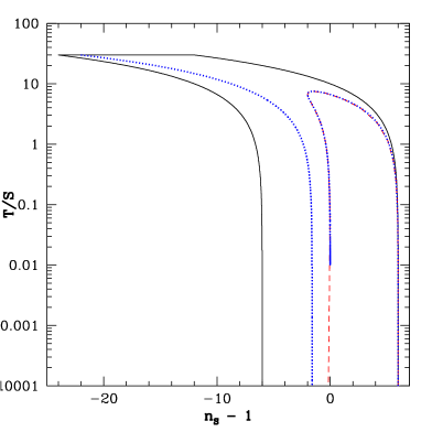
Figure 1: The SR validity region (solid black line) flown back 50 e-folds (dashed red line) together with two examples of flow lines (blue dashed lines) ending on the boundary of the SR validity region. In this case we set $\xi^{2}=0$.

In order to close the set of equations, so that the flow equations uniquely define the time evolution of $n_{S}$ and $n_{T}$, we need to introduce an additional constraint, and there are various possibilities. In ref. [Hoffman & Turner 2001] the assumption was made that $x^{\prime\prime}=0$, where $x=V^{\prime}/V$. Another possibility would be to assume that either $V^{\prime\prime\prime}/V$ or $\xi^{2}$ can be treated as constants. Different choices will lead to different fix-points and different time evolution of $n_{S}$ and $n_{T}$, and general conclusions are therefore only credible if such conclusions are reached for any choice of this additional constraint.

Observational constraints. The COBE observations [Bunn, Liddle & White 1996] gave the first constraint on the first derivative

$$\frac{V^{3/2}}{M^{3}V^{\prime}}\approx 5\times 10^{-4}\,,$$ (9)

and the present day constraints on slow roll parameters are improved when combining CMB data with data from the Lyman-$\alpha$ forest. The reason being that the error-ellipses for CMB and Lyman-$\alpha$ are almost perpendicular [Hannestad et al. 2002]. The reason for using Lyman-$\alpha$ data [Croft et al. 2000] instead of “standard” LSS data (such as PSCz [Saunders et al. 2000] or 2dFGRS [Percival et al. 2001]) is, that the Lyman-$\alpha$ data are obtained at high red-shift, where small scales are still linear. One should naturally keep in mind, that neither CMB nor Ly-$\alpha$ data include all the possible systematic errors. The bounds obtained are [Hannestad et al. 2002] (all at $2\sigma$)

$$0.8< n_{s} <1.0\,,$$ (10)

$$0< r <0.3\,,$$ (11)

$$-0.05< \partial_{{\rm ln}k} <0.02\,,$$ (12)

where $n_{S}$ is the scalar spectral index, $r$ is the tensor to scalar ratio, and $\partial_{{\rm ln}k}=dn_{S}/d{\rm ln}k$ is the bend defined through eq. (1). These bounds directly provide constraints on the first and second derivatives of the potential,

$$M\left|\frac{V^{\prime}}{V}\right| < 0.25\,,$$ (13)

$$M^{2}\left|\frac{V^{\prime\prime}}{V}\right| < 0.1\,,$$ (14)

however, the third derivative is not directly constrained. Instead, eqs. (10-12) limit only $\xi^{2}$ to be smaller than about $|\xi^{2}|<0.036$, when assuming independent errors on $n_{S},r$ and $dn_{S}/d{\rm ln}k$, and in reality one could obtain a slightly stronger bound. To obtain a bound on $V^{\prime\prime\prime}$ we must combine the observational constraints (10-12) with the flow equations in SR parameter space, eqs. (6,7). This is because one has $dn_{S}/d{\rm ln}k\approx\sqrt{r}\,(V^{\prime\prime\prime}/V)\,(-2M^{3}/\sqrt{\kappa})+4r/\kappa\,[n_{S}-1+3/2\,r/\kappa]$, and since we don’t have a lower bound on $r$ we cannot get any direct constraint on $V^{\prime\prime\prime}/V$.

3 Discussion

We are going to consider the case, where slow-roll inflation is ended because the slow-roll conditions are violated, eq. (8). Another possibility would be to allow for other fields coupled to the inflaton field which could end inflation. The parameters observable with CMB and LSS are determined approximately 50 e-folds before the end of inflation, and we therefore run the SR violating boundary back in time 50 e-folds. This is done for various values of fixed $\xi^{2}$ (or fixed $V^{\prime\prime\prime}/V$). Now we demand that the observable parameters be in agreement with eq. (10), and if no point on the SR violating boundary lands inside the observed parameter-range, then we can exclude this value of $\xi^{2}$ (or $V^{\prime\prime\prime}/V$).

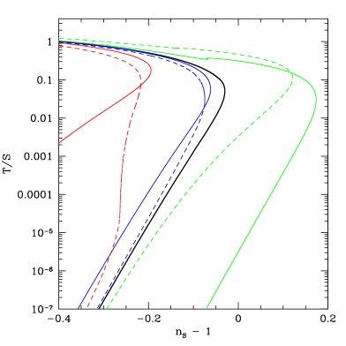
Figure 2: Examples of the flown back SR validity boundary, 50 e-folds before the end of inflation. The thicker solid black line shows the case for $\xi^{2}=0$. For the solid lines, $\xi^{2}$ was kept constant, while the dashed lines are for models where $V^{\prime\prime\prime}/V$ was kept constant. From left to right we show examples for $\xi^{2}=-10^{-2}$, $-10^{-3}$ and $+5\times 10^{-3}$ as well as $V^{\prime\prime\prime}/V=-5\times 10^{-2}$, $-10^{-2}$ and $+5\times 10^{-2}$. For small $r=T/S$ the models with constant $\xi^{2}$ move nearly parallel to the $n_{S}$ direction while the ones with constant $V^{\prime\prime\prime}/V$ are frozen and remain close to the $\xi^{2}=0$ curve.

Let us first consider the case where $\xi^{2}$ can be treated as a constant during the 50 e-folds. If $\xi^{2}=0$ one finds, that 50 e-folds before the crossing of the SR violating boundary one has

$$2\times 10^{-5}<r<0.5\,,$$ (15)

when we demand that $n_{s}$ complies with eq. (10). This can also be seen in fig. 2, where the thicker solid line is for $\xi^{2}=0$. If $\xi^{2}$ is positive then $r$ must be even smaller, since the region in fig. 2 moves to the right (larger $n_{s}$), and for $\xi^{2}>0.06$ there are no more points in agreement with observations. For negative $\xi^{2}$ the acceptable values of $r$ are larger than $2\times 10^{-5}$, and for $\xi^{2}<-0.06$ there are no points in agreement with observations. We hence conclude, that in the case where $\xi^{2}$ can be considered constant throughout the 50 e-folds and inflation ends by violating the slow-roll conditions, one must have $|\xi^{2}|<0.06$. We therefore find a constraint on $\partial_{{\rm ln}k}$ similar to (12) from the observational constraints on $n_{s}$ and the flow equations alone. This bound on $\xi^{2}$ can be converted into a bound on $V^{\prime\prime\prime}/V$ using the predicted $r$ and the relation $\xi^{2}=\sqrt{r/\kappa}M^{3}V^{\prime\prime\prime}/V$. We find $M^{3}V^{\prime\prime\prime}/V>-0.2$.

If one instead considers the case where $V^{\prime\prime\prime}/V$ can be treated as a constant during the 50 e-folds, then the conclusions are slightly different. Again, in the case with $V^{\prime\prime\prime}/V=0$ one finds $2\times 10^{-5}<r<0.5$. When $V^{\prime\prime\prime}/V$ is negative then no points agree with observations if $V^{\prime\prime\prime}/V<-0.05$. Only for positive $V^{\prime\prime\prime}/V$ there will always be acceptable points, however, the allowed range for $r$ will decrease, e.g. for $M^{3}V^{\prime\prime\prime}/V=1$ one finds $10^{-7}<r<10^{-5}$.

As discussed above, the most credible results must agree independently of the additional constraint (fixed $\xi^{2}$ or fixed $V^{\prime\prime\prime}/V$). We have seen that one always finds a lower bound

$$\frac{V^{\prime\prime\prime}}{V}>-0.2\,.$$ (16)

This is the first constraint found on the third derivative of the inflaton potential, and is valid under the assumptions specified above. It is important to note, that the approach adopted here differs from the results of ref. [Liddle & Turner 1994], where it was pointed out, that an observation of $\partial_{{\rm ln}k}$ would provide knowledge about $V^{\prime\prime\prime}$. The difference being, that in our case we have only an observational upper bound on $r$, and without the use of the flow equations, this will leave $V^{\prime\prime\prime}$ completely unknown.

No strong predictions can be made on the magnitude of $r$, simply because if $V^{\prime\prime\prime}/V$ is large then $r$ is allowed to be smaller, however, one would often expect $M^{3}V^{\prime\prime\prime}/V$ to be smaller than both $M^{2}V^{\prime\prime}/V$ and $MV^{\prime}/V$, eqs. (13,14), in which case one predicts $r>3\times 10^{-6}$.

The number of e-folds $N$ depends on the detailed mechanism of inflation such as the reheat temperature and the energy scale of inflation, and can be somewhat different from 50 (see e.g. [Lyth & Riotto 1999]). If $N=60$ our direct bound on $V^{\prime\prime\prime}/V>-0.05$ remains unchanged, however, the inferred bound from the case of constant $\xi^{2}$ is weakened by approximately a factor of 2. The lower bound on r discussed above becomes $r>3\times 10^{-7}$. Naturally, for a lower value of $N$ the bounds are correspondingly stronger.

4 Conclusion

COBE gave us the first clear information on the first derivative of the inflaton potential, and the combination of CMB observations with data from the Lyman-$\alpha$ forest has given us information on the first two derivatives of the inflaton potential. Here we have combined the present observations with the flow equations in slow roll space, and found a lower bound on the third derivative of the inflaton potential $V^{\prime\prime\prime}/V>-0.2$. We have also shown, that unless $V^{\prime\prime\prime}/V$ is unreasonably large, then one predicts the tensor to scalar ratio, $r$, to be bounded from below $3\times 10^{-6}<r$.

References

- [Bunn, Liddle & White 1996] Bunn E. F., Liddle A. R., White M. J., 1996, Phys. Rev. D 54, 5917.
- [Copeland, Grivell & Liddle 1997] Copeland E. J., Grivell I. J., Liddle A. R., 1997, astro-ph/9712028.
- [Covi & Lyth 1999] Covi L., Lyth D. H., 1999, Phys. Rev. D59, 063515.
- [Croft et al. 2000] Croft R. A. et al., 2000, astro-ph/0012324.
- [Dodelson, Kinney & Kolb 1997] Dodelson S., Kinney W. H., Kolb E. W., 1997, Phys. Rev. D56, 3207.
- [Dodelson & Stewart 2002] Dodelson S., Stewart E., 2002, Phys. Rev. D65, 101301.
- [Halverson et al. 2002] Halverson N. W. et al., 2002, Astrophys. J. 568, 38.
- [Hannestad, Hansen & Villante 2001] Hannestad S., Hansen S. H., Villante F. L., 2001, Astropart. Phys. 16, 137.
- [Hannestad et al. 2002] Hannestad S., Hansen S. H., Villante F. L., Hamilton A. J., 2002, Astropart. Phys. 17, 375.
- [Hoffman & Turner 2001] Hoffman M. B., Turner M. S., 2001, Phys. Rev. D 64, 023506.
- [Kinney & Riotto 1998] Kinney W. H., Riotto A., 1998, Phys. Lett. B435, 272.
- [Kinney, Melchiorri & Riotto 2001] Kinney W. H., Melchiorri A., Riotto A., 2001, Phys. Rev. D 63, 023505.
- [Knox 1995] Knox L., 1995, Phys. Rev. D 52, 4307.
- [Kolb & Turner 1990] Kolb E. W., Turner M. S., 1990, Redwood City, USA: Addison-Wesley (1990) 547 p. (Frontiers in physics, 69).
- [Kosowsky & Turner 1995] Kosowsky A., Turner M. S., 1995, Phys. Rev. D 52, 1739.
- [Lee et al. 2001] Lee A. T. et al., 2001, Astrophys. J. 561, L1.
- [Liddle & Lyth 1992] Liddle A. R., Lyth D. H., 1992, Phys. Lett. B291, 391.
- [Liddle & Turner 1994] Liddle A. R., Turner M. S., 1994, Phys. Rev. D50, 758 [Erratum-ibid. D54, 2980].
- [Lidsey et al. 1997] Lidsey J. E., Liddle A. R., Kolb E. W., Copeland E. J., Barreiro T., Abney M., 1997, Rev. Mod. Phys. 69, 373.
- [Lyth & Riotto 1999] Lyth D. H., Riotto A., 1999, Phys. Rept. 314, 1.
- [Netterfield et al. 2002] Netterfield C. B. et al., 2002, Astrophys. J. 571, 604.
- [Percival et al. 2001] Percival W. J. et al., 2001,Mon. Not. R. Astron. Soc., 327, 1297.
- [Saunders et al. 2000] Saunders W. et al., 2000, Mon. Not. R. Astron. Soc., 317, 55.
- [Stewart 1997] Stewart E. D., 1997, Phys. Lett. B391, 34.
- [Stewart 1997b] Stewart E. D., 1997, Phys. Rev. D56, 2019.
- [Terrero-Escalante & Garcia 2002] Terrero-Escalante C. A., Garcia A. A., 2002, Phys. Rev. D 65, 023515.
- [Turner & White 1996] Turner M. S., White M., 1996, Phys. Rev. D53, 6822.
- [Wang, Tegmark & Zaldarriaga 2002] Wang X., Tegmark M., Zaldarriaga M., 2002, Phys. Rev. D65, 123001.