September, 2001

hep-ph/0109244

OU-HET 396

$\bar{B}\to D\tau\bar{\nu}_{\tau}$ in two-Higgs-doublet models

Takahiro MIURA and Minoru TANAKA
Department of Physics, Osaka University
Toyonaka, Osaka 560-0043, Japan

We study the exclusive semi-tauonic $B$ decay, $\bar{B}\to D\tau\bar{\nu}_{\tau}$, in two-Higgs-doublet models. Using recent experimental and theoretical results on hadronic form factors, we estimate theoretical uncertainties in the branching ratio. As a result, we clarify the potential sensitivity of this mode to the charged Higgs exchange. Our analysis will help to probe the charged Higgs boson at present and future B factory experiments.

1 Introduction

Many interesting models for the new physics beyond the standard model (SM) have been considered. One of the most attractive models is the minimal supersymmetric standard model (MSSM) [1]. In the MSSM, two Higgs doublets are introduced in order to cancel the anomaly and to give the fermions masses. The introduction of the second Higgs doublet inevitably means that a charged Higgs boson is in the physical spectra. So, it is very important to study effects of the charged Higgs boson.

Here, we study effects of the charged Higgs boson on the exclusive semi-tauonic $B$ decay, $\bar{B}\to D\tau\bar{\nu}_{\tau}$, in the MSSM. In a two-Higgs-doublet model, we have a pair of charged Higgs bosons, $H^{\pm}$, and its couplings to quarks and leptons are given by

$${\cal L}_{H} = (2\sqrt{2}G_{F})^{1/2}\bigl{[}X\overline{u}_{L}V_{KM}M_{d}d_{R}+Y\overline{u}_{R}M_{u}V_{KM}d_{L}+Z\overline{\nu}_{L}M_{l}l_{R}\bigr{]}\;H^{+}$$ (1)

$$+\mbox{\large h.c.}\;,$$

where $M_{u}$, $M_{d}$ and $M_{l}$ are diagonal quark and lepton mass matrices, and $V_{KM}$ is Kobayashi-Maskawa matrix [2]. In the MSSM, we obtain

$$X=Z=\tan\beta\;,\;\;Y=\cot\beta\;,$$ (2)

where $\tan\beta=v_{2}/v_{1}$ is the ratio of the vacuum expectation values of the Higgs bosons. Since the Yukawa couplings of the MSSM are the same as those of the so-called Model II of two-Higgs-doublet models [3], the above equations and the following results apply to the latter as well.

From these couplings, we observe that the amplitude of charged Higgs exchange in $\bar{B}\to D\tau\bar{\nu}_{\tau}$ has a term proportional to $m_{b}\tan^{2}\beta$. Thus, the effect of the charged Higgs boson is more significant for larger $\tan\beta$.

In Sec.2, we give formula of the decay rate. The employed hadronic form factors are described in Sec.3. In Sec.4, we show our numerical results. Sec.5 is devoted to conclusion.

2 Formula of the decay rate

Using the above Lagrangian in Eq.(1) and the standard charged current Lagrangian, we can calculate the amplitudes of charged Higgs exchange and $W$ boson exchange in $\bar{B}\to D\tau\bar{\nu}_{\tau}$.

The $W$ boson exchange amplitude is given by [4]

$${\cal M}_{s}^{\lambda_{\tau}}(q^{2},x)_{W}=\frac{G_{F}}{\sqrt{2}}V_{cb}\sum_{\lambda_{W}}\eta_{\lambda_{W}}L_{\lambda_{W}}^{\lambda_{\tau}}H_{\lambda_{W}}^{s}\;,$$ (3)

where $q^{2}$ is the invariant mass squared of the leptonic system, and $x=p_{B}\cdot p_{\tau}/m_{B}^{2}$. The $\tau$ helicity and the virtual $W$ helicity are denoted by $\lambda_{\tau}=\pm$ and $\lambda_{W}=\pm,\,0,\,s$, and the metric factor $\eta_{\lambda_{W}}$ is given by $\eta_{\pm}=\eta_{0}=-\eta_{s}=1$. The hadronic amplitude which describes $\bar{B}\rightarrow D\,W^{*}$ and the leptonic amplitude which describes $W^{*}\rightarrow\tau\bar{\nu}$ are given by

$$H_{\lambda_{W}}^{s}(q^{2}) \equiv \epsilon_{\mu}^{*}(\lambda_{W})\langle D(p_{D})|\bar{c}\gamma^{\mu}b|\bar{B}(p_{B})\rangle\;,$$ (4)

$$L_{\lambda_{W}}^{\lambda_{\tau}}(q^{2},x) \equiv \epsilon_{\mu}(\lambda_{W})\langle\tau(p_{\tau},\lambda_{\tau})\bar{\nu}_{\tau}(p_{\nu})|\bar{\tau}\gamma^{\mu}(1-\gamma_{5})\nu_{\tau}|0\rangle\;,$$ (5)

where $\epsilon_{\mu}(\lambda_{W})$ is the polarization vector of the virtual $W$ boson.

The charged Higgs exchange amplitude is given by [5]

$${\cal M}_{s}^{\lambda_{\tau}}(q^{2},x)_{H}=\frac{G_{F}}{\sqrt{2}}V_{cb}L^{\lambda_{\tau}}\Bigl{[}XZ^{*}\frac{m_{b}m_{\tau}}{M_{H}^{2}}H_{R}^{s}+YZ^{*}\frac{m_{c}m_{\tau}}{M_{H}^{2}}H_{L}^{s}\Bigr{]}\;.$$ (6)

Here, the hadronic and leptonic amplitudes are defined by

$$H_{R,L}^{s}(q^{2}) \equiv \langle D(p_{D})|\bar{c}(1\pm\gamma_{5})b|\bar{B}(p_{B})\rangle\;,$$ (7)

$$L^{\lambda_{\tau}}(q^{2},x) \equiv \langle\tau(p_{\tau},\lambda_{\tau})\bar{\nu}_{\tau}(p_{\nu})|\bar{\tau}(1-\gamma_{5})\nu_{\tau}|0\rangle\;.$$ (8)

These amplitudes are related to the $W$ exchange amplitudes as

$$H_{R,L}^{s}=\frac{\sqrt{q^{2}}}{m_{b}-m_{c}}H_{s}^{s}\;,\;\;L^{\lambda_{\tau}}=\frac{\sqrt{q^{2}}}{m_{\tau}}L^{\lambda_{\tau}}_{s}\;,$$ (9)

where the former relation is valid in the heavy quark limit.

Using the amplitudes of Eqs.(3) and (6), the differential decay rate is given by

$$\frac{d\Gamma}{dq^{2}} = \frac{G_{F}^{2}|V_{cb}|^{2}v^{4}\sqrt{Q_{+}Q_{-}}}{128\pi^{3}m_{B}^{3}}\Bigl{[}\Bigl{(}\frac{2}{3}q^{2}+\frac{1}{3}m_{\tau}^{2}\Bigr{)}(H^{s}_{0})^{2}\Bigr{.}$$

. $$+m_{\tau}^{2}\Bigl{(}\frac{q^{2}\tan^{2}\beta}{M_{H}^{2}}\frac{m_{b}}{m_{b}-m_{c}}+\frac{q^{2}}{M_{H}^{2}}\frac{m_{c}}{m_{b}-m_{c}}-1\Bigr{)}^{2}(H_{s}^{s})^{2}\Bigr{]}\;,$$ (10)

where $Q_{\pm}=(m_{B}\pm m_{D})^{2}-q^{2}$ and $v=\sqrt{1-m_{\tau}^{2}/q^{2}}$. Note that if $\tan\beta\gtrsim 1$, in which we are interested, this decay rate is practically a function of $\tan\beta/M_{H}$ because the second term in the coefficient of $(H^{s}_{s})^{2}$ is negligible for $m_{b}\tan^{2}\beta\gg m_{c}$.

3 Hadronic form factors

In order to obtain the decay rate numerically, it is necessary to calculate the hadronic amplitude in Eq.(4). This amplitude is given in terms of hadronic form factors:

$$\langle D(p_{D})|\bar{c}\gamma^{\mu}b|\bar{B}(p_{B})\rangle=\sqrt{m_{B}m_{D}}\bigl{[}h_{+}(y)(v+v^{\prime})^{\mu}+h_{-}(y)(v-v^{\prime})^{\mu}\bigr{]}\;,$$ (11)

where $v=p_{B}/m_{B}$, $v^{\prime}=p_{D}/m_{D}$ and $y\equiv v\cdot v^{\prime}=(m_{B}^{2}+m_{D}^{2}-q^{2})/2m_{B}m_{D}$ [6].

In the heavy quark limit and in the leading logarithmic approximation, $h_{+}(y)$ and $h_{-}(y)$ are given as

$$h_{+}(y)=\xi(y)\;,\;\;h_{-}(y)=0\;,$$ (12)

where $\xi(y)$ is the universal form factor [7].

The form of $\xi(y)$ is constrained strongly by the dispersion relations as [8]

$$\xi(y)\simeq 1-8\rho_{1}^{2}z+(51.\rho_{1}^{2}-10.)z^{2}-(252.\rho_{1}^{2}-84.)z^{3}\;,$$ (13)

where $z=(\sqrt{y+1}-\sqrt{2})/(\sqrt{y+1}+\sqrt{2})$. To determine the slope parameter $\rho_{1}^{2}$, we use the experimental data of Belle [9], and we obtain

$$\rho_{1}^{2}=1.33\pm 0.22\;.$$ (14)

This error of $\rho_{1}^{2}$ dominantly contributes to the uncertainty in the theoretical calculation of the branching ratio.

4 Numerical results

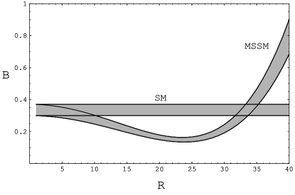
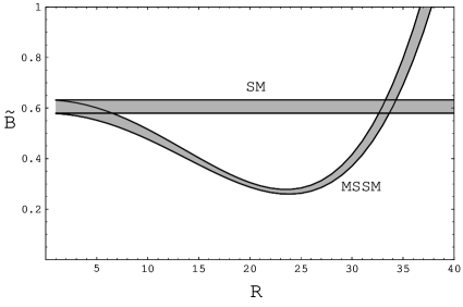
Figure 1: The ratios $B$ and $\tilde{B}$ as functions of $R$ in the MSSM and the SM. The shaded regions show the predictions with the error in the slope parameter $\rho_{1}^{2}$ in Eq.(14). The flat bands show the SM predictions. (a) $B$: the decay rate normalized to $\Gamma(\bar{B}\rightarrow D\mu\bar{\nu}_{\mu})_{SM}$. (b) $\tilde{B}$: the same as (a) except that the denominator is integrated over $m_{\tau}^{2}\leq q^{2}\leq(m_{B}-m_{D})^{2}$.

Now, we consider the following ratio,

$$B=\frac{\Gamma(\bar{B}\rightarrow D\tau\bar{\nu}_{\tau})}{\Gamma(\bar{B}\rightarrow D\mu\bar{\nu}_{\mu})_{SM}}\;,$$ (15)

where the denominator is the decay rate of $\bar{B}\rightarrow D\mu\bar{\nu}_{\mu}$ in the SM, since the uncertainties due to the form factors and other parameters tend to reduce or vanish by taking the ratio.

Fig.1(a) is the plot of our predictions of the ratio in Eq.(15) as a function of $R$, which is defined by $R\equiv m_{W}\tan\beta/m_{H}$. The shaded regions show the MSSM and SM predictions with the error in the slope parameter $\rho_{1}^{2}$ in Eq.(14). As seen in Fig.1(a), when $R$ reaches about 32, the branching ratio in the MSSM becomes the same as the one in the SM. It is because the interference of the W exchange and the charged Higgs exchange is negative. From Fig.1(a), we expect that the experimentally possible sensitivity of $R$ is $\sim 10$, provided that the error in $\rho_{1}^{2}$ will not change.

In Fig.1(b), we also show the ratio,

$$\tilde{B}=\frac{\Gamma(\bar{B}\rightarrow D\tau\bar{\nu}_{\tau})}{\tilde{\Gamma}(\bar{B}\rightarrow D\mu\bar{\nu}_{\mu})_{SM}}\;,$$ (16)

the same as Fig.1(a), but its denominator is $\tilde{\Gamma}(\bar{B}\rightarrow D\mu\bar{\nu}_{\mu})_{SM}$, which is integrated over the same $q^{2}$ region as the $\tau$ mode, i.e., $m_{\tau}^{2}\leq q^{2}\leq(m_{B}-m_{D})^{2}$. From Fig.1(b), we expect less theoretical uncertainty and a better sensitivity of $\tilde{B}$ compared with $B$ in Fig.1(a).

Figure 2: (a) The contour plot of upper bound of $R$ at $90\%$ CL as a function of $\delta\rho_{1}^{2}$ and $\delta B_{exp}$. (b) The same as (a) except that the ratio in Eq.(16) is used.

Once the experimental values of $B$ ($\tilde{B}$), its error $\delta B$ ($\delta\tilde{B}$), $\rho_{1}^{2}$ and its error $\delta\rho_{1}^{2}$ are given, we can obtain a bound on $R$. In the following, we assume the SM prediction as the experimental value of $B$ ($\tilde{B}$) , i.e., $B_{exp}=B_{SM}\pm\delta B_{exp}$ ($\tilde{B}_{exp}=\tilde{B}_{SM}\pm\delta\tilde{B}_{exp}$), and we use the central value of Eq.(14) as the input of the slope parameter.

Fig.2(a) is the contour plot of upper bound of $R$ at $90\%$ CL as a function of $\delta\rho_{1}^{2}$ and $\delta B_{exp}$. From this figure, if $\delta B_{exp}=0$, and $\delta\rho_{1}^{2}\sim 17\%$, which corresponds to the present experimental error in Eq.(14), we expect that an upper bound of $R\sim 10$, which is consistent with the result of Fig.1(a). If we will observe $\bar{B}\rightarrow D\tau\bar{\nu}_{\tau}$ with $\delta B_{exp}\simeq 20\%$, we expect that an upper bound of $R\sim 15$ weakly depending on $\delta\rho_{1}^{2}$.

In Fig.2(b), we also show a similar contour plot where we use the ratio defined in Eq.(16), i.e., normalized to $\tilde{\Gamma}(\bar{B}\rightarrow D\mu\bar{\nu}_{\mu})_{SM}$. We observe that the upper bound of R is almost independent of $\delta\rho_{1}^{2}$ in this case. Thus, it is important to make the experimental error in $B$ ($\tilde{B}$), $\delta B_{exp}$ ($\delta\tilde{B}_{exp}$), small rather than $\delta\rho_{1}^{2}$.

5 Conclusion

As seen in our numerical results, the branching ratio of $\bar{B}\rightarrow D\tau\bar{\nu}_{\tau}$ is a sensitive probe of the MSSM-like Higgs sector. We expect an upper bound of $R\lesssim 15$ when $\delta B_{exp}\simeq 20\%$ is achieved. So, if $\bar{B}\rightarrow D\tau\bar{\nu}_{\tau}$ is observed at a B factory experiment, a significant regions of the parameter space of the MSSM Higgs sector will be covered. Comparing with the Higgs search scenario of LHC [10], we conclude that present and future B factories are potentially competitive with LHC.

As future improvements of the present work, the $q^{2}$ distribution [11] and the $\tau$ polarization [5] of $\bar{B}\rightarrow D\tau\bar{\nu}_{\tau}$ are promising. In these quantities, we will expect that the theoretical uncertainties from the error in the slope parameter become very small. However, we should take 1/m and QCD corrections into account. These corrections are neglected in the present work because they lead to smaller uncertainties than those from $\delta\rho_{1}^{2}$. For the $q^{2}$ distribution and the $\tau$ polarization, they are expected to be dominant uncertainties in the theoretical calculations. These issues will be addressed elsewhere.

References

[1]
For a review, see, e.g.,
H. E. Haber and G. L. Kane, Phys. Rep. 117 (1985) 75.
[2]
M. Kobayashi and T. Maskawa, Prog. Theor. Phys. 49 (1973) 652.
[3]
J. F. Gunion, H. E. Haber, G. L. Kane and S. Dawson,
The Higgs Hunter’s Guide
(Addison-Wesley Publishing Company, 1990).
[4]
K. Hagiwara, A. D. Martin and M. F. Wade, Nucl. Phys. B327 (1989) 569;
K. Hagiwara, A. D. Martin and M. F. Wade, Z. Phys. C46 (1990) 299.
[5]
M. Tanaka, Z. Phys. C67 (1995) 321.
[6]
M. Neubert, Phys. Lett. B264 (1991) 455.
[7]
N. Isgur and M. B. Wise, Phys. Lett. B232 (1989) 113; Phys. Lett. B237 (1990) 527.
[8]
I. Caprini, L. Lellouch and M. Neubert, Nucl. Phys. B530 (1998) 153.
[9] K. Abe et.al., BELLE-CONF-0121 (2001).
[10] F. Gianotti, talk presented at LHCC, 5 July, 2000,
http://gianotti.home.cern.ch/gianotti/phys_info.html .
[11] K. Kiers and A. Soni, Phys. Rev. D56 (1997) 5786.