Freezing of the QCD coupling constant and solutions of Schwinger-Dyson equations

Abstract

We compare phenomenological values of the frozen QCD running coupling constant ($\alpha_{s}$) with two classes of solutions obtained through nonperturbative Schwinger-Dyson equations. We use these same solutions with frozen coupling constants as well as their respective nonperturbative gluon propagators to compute the QCD prediction for the asymptotic pion form factor. Agreement between theory and experiment on $\alpha_{s}(0)$ and $F_{\pi}(Q^{2})$ is found only for one of the solutions Schwinger-Dyson equations.

]

I Introduction

The possibility that the QCD coupling constant ($\alpha_{s}$) has an infrared (IR) finite behavior has been extensively studied in recent years. There are theoretical arguments in favor of the coupling constant freezing at low momenta, one of them, à la Banks and Zaks[1], claims that QCD may have a non-trivial IR fixed point even for a small number of quarks (see, for instance, Ref.[2]). We can also use arguments of analyticity to show that the analytical coupling freezes at the value of $4\pi/\beta_{0}$[3], where $\beta_{0}$ is the one-loop coefficient of the QCD $\beta$ function.

Studies of the nonperturbative QCD vacuum also indicate the existence of a finite coupling constant in the IR[4, 5].

The phenomenological evidences for the strong coupling constant freezing in the IR are much more numerous. Models where a static potential is used to compute the hadronic spectra make use of a frozen coupling constant at long distances[6, 7].

Heavy quarkonia decays and total hadron-hadron cross sections are influenced by the freezing of the coupling constant[8].

A quite detailed analysis of the ratio $R_{e^{+}e^{-}}$ ($\equiv\sigma_{tot}(e^{+}e^{-}\rightarrow hadrons)/\sigma(e^{+}e^{-}\rightarrow\mu^{+}\mu^{-})$)performed by Mattingly and Stevenson[9] also shows a signal for the freezing of the QCD coupling. Following an almost similar study, for several hadronic observables, Dokshitzer and Webber obtain the same result[10].

Another method to investigate the infrared behavior of gluon and ghost propagators, and of the running coupling constant at low energies is through the solution of the Schwinger-Dyson equations (SDE)[11]. Early studies of the SDE for the gluon propagator in the Landau gauge concluded that the gluon propagator is highly singular in the infrared[12]. However, these results are discarded by simulations of QCD on the lattice at $95\%$ confidence level[13], where it is shown that the gluon propagator probably is infrared finite. The lattice result is in agreement with two classes of SDE solutions. One proposed by Cornwall many years ago where the gluon acquires a dynamical mass[14], and another that has been extensively discussed by Alkofer and von Smekal where the gluon propagator goes to zero when the momentum $q^{2}\rightarrow 0$[15]. The solutions differ due to the different approximations performed to solve the SDE, but in both cases there is a freezing of the coupling constant in the IR.

Although the figures of the most recent lattice calculation[13] seems to indicate that the Cornwall’s gluon propagator is the one that could better explain the results, it is correct to say that the data is still not precise enough in the IR region to decide among the two possible behaviors for the gluon propagators discussed in the previous paragraph. The purpose of our work is exactly to confront the IR values of the theoretical coupling constant, obtained with the solutions of the SDE, with the phenomenological data about the value of $\alpha_{s}(0)$ in order to discriminate which one is the most suitable solution. Finally, these theoretical and phenomenological calculations are outside the scope of standard perturbation theory, and a consistency check between them is the minimum that we may require to know if these approaches make sense at all. In the next section we present the expressions of the nonperturbative running coupling constant obtained with the SDE study, and compare them with some of the phenomenological values obtained for $\alpha_{s}(0)$. In Section III we compute the pion form factor ($F_{\pi}(Q^{2})$) as a function of these coupling constants. It is known that $F_{\pi}(Q^{2})$ is quite dependent on the behavior of $\alpha_{s}$ at small momentum[16].

Therefore, this calculation provides a good test for the nonperturbative expression of the QCD coupling constant. Considering that solutions of SDE show a nonperturbative behavior for the infrared coupling as well as for the gluon propagators, in Section IV we modify the expression for the asymptotic pion form factor to take into account these nonperturbative gluon propagators. In the last section we present our discussion and conclusions.

II The phenomenological value of $\alpha_{s}(0)$

At high energies it is believed that the property of asymptotic freedom allow us to perform reliable QCD calculations. However, the same is not true at low energies, where we have to make use of a series of phenomenological models when computing strong interaction parameters.

This is exactly what happens if we want to determine the IR behavior of the running coupling constant. We are going to present some of the determinations of $\alpha_{s}(0)$, and the most impressive fact is that the values obtained in several different analysis are not far apart by one order of magnitude, but they differ at most by a factor of two, providing a solid indication of the robustness of these approaches.

One of the most detailed calculation of $\alpha_{s}(0)$ is due to Mattingly and Stevenson[9], which uses perturbation theory and renormalization group invariance to compute $R_{e^{+}e^{-}}$ up to third order in $\alpha_{s}$. They predict the value

$$\alpha_{s}/\pi=0.26,$$ (1)

($\alpha_{s}(0)=0.82$) for the frozen IR coupling. On the other hand the long work of Ref.[10] gives

$$\alpha_{s}(0)\approx 0.63.$$ (2)

The analysis of hadronic spectroscopy with potential models by Godfrey and Isgur[7] led to the following behavior of the coupling constant

$$\alpha_{gi}=0.25\exp( -q^{2})+0.15\exp(-0.1q^{2})$$ (4)

$$+0.20\exp(-0.001q^{2}),$$

where $q$ is in GeV (all the momenta, otherwise specified, will be in Euclidean space), and a good fit of the spectra does not depend strongly on the ultraviolet behavior of the coupling constant. From the above equation we obtain $\alpha_{s}(0)=0.60$. Which is also consistent with more recent studies of QCD potentials[17]. Analysis of $e^{+}e^{-}$ annihilation, as well as bottomonium and charmonium fine structure in the framework of the background perturbation theory may lead to a frozen value of the coupling constant as low as $\alpha_{s}(0)\approx 0.4$[19]. This method also explains the frozen value of $\alpha_{s}$ resulting from the lattice simulation of the short range static potential[20], and it gives

$$\alpha_{B}(0)\approx\frac{4\pi}{\beta_{0}\ln{\frac{m^{2}_{B}}{\Lambda^{2}_{V}}}},$$ (5)

where $m_{B}$ is a background mass. This one and $\Lambda_{V}$ (with $m_{B}>\Lambda_{V}$) are determined phenomenologically[20].

There are many other results that we could present here, but we can assume that the phenomenological values of $\alpha_{s}(0)$ scattered in the literature are in the range

$$\alpha_{s}(0)\approx 0.7\pm 0.3.$$ (6)

Although this choice is ad hoc, as far as we know it contemplates most of the phenomenological determinations of $\alpha_{s}(0)$.

We now turn to the coupling constants obtained through the SDE solutions. The first nonperturbative running coupling constant that we shall discuss was obtained by Cornwall[14], using the pinch technique to derive a gauge invariant SDE. This nonperturbative coupling is equal to

$$\alpha_{sC}(q^{2})=\frac{4\pi}{\beta_{0}\ln\left[(q^{2}+4M_{g}^{2}(q^{2})/\Lambda^{2}\right]},$$ (7)

where $M_{g}(q^{2})$ is a dynamical gluon mass given by,

$$M^{2}_{g}(q^{2})=m_{g}^{2}\left[\frac{\ln\left(\frac{q^{2}+4{m_{g}}^{2}}{\Lambda^{2}}\right)}{\ln\left(\frac{4{m_{g}}^{2}}{\Lambda^{2}}\right)}\right]^{-12/11}$$ (8)

$\Lambda$($\equiv\Lambda_{QCD}$) is the QCD scale parameter, $\beta_{0}=11-\frac{2}{3}n_{f}$, where $n_{f}$ is the number of flavors. In the above expression we are neglecting the effect of dynamical or bare fermions masses[14]. We can determine $\alpha_{s}(0)$ in Eq.(7) as a function of the gluon mass $m_{g}$ and $\Lambda$, and these ones can be obtained in the calculation of several hadronic parameters that may vary with $m_{g}$ (but, in general, not strongly with the ratio $m_{g}/\Lambda$). A typical value is[14, 18]

$$m_{g}=500\pm 200\quad{\textnormal{M}eV}$$ (9)

for $\Lambda=300$ MeV. It is interesting to observe the similarity between Eq.(7) and Eq.(5). Although, it is not clear to us the reason for this similarity.

The other possibility for the IR finite running coupling was studied by Alkofer et al. [15], that solved a coupled set of SDE for the propagators of gluons and ghosts. In this approach the solution to the running coupling leads to an infrared fixed point, which, in terms of the invariant functions $Z(k^{2})$ and $G(k^{2})$ related to the renormalization of gluon and ghost propagators respectively, is given by

$$\alpha_{s}(\mu)=\frac{g^{2}}{4\pi\beta_{0}}Z(\mu^{2})G^{2}(\mu^{2})|_{\mu\rightarrow 0}$$ (10)

$$=\frac{16\pi}{3N_{c}}\left(\frac{1}{\kappa}-\frac{1}{2}\right)^{-1}\simeq 9.5.$$ (11)

with ${\kappa}=0.92$.

The above result gives $\alpha_{s}$ near the origin. It has been obtained for $n_{f}=0$. As we are going to compare different SDE solutions we will limit ourselves to the flavorless, or pure gauge, QCD. The effect of $n_{f}\neq 0$ will be discussed in the last section.

Since we shall use the running coupling in the full range of momenta we provide a fit for the numerical data of Ref.[15], given by the following expression:

$$\alpha_{sA}=\left\{\begin{array}[]{l@{\quad:\quad}l}\alpha_{sA1}&q^{2}<0.31\;{\textnormal{G}eV}^{2}\\ \alpha_{sA2}&0.31<q^{2}<1.3\;{\textnormal{G}eV}^{2}\\ \alpha_{sA3}&q^{2}>1.3\;{\textnormal{G}eV}^{2}\end{array}\right.$$ (15)

with

$$\alpha_{sA1} = 0.2161+9.2621\exp\left(-2\frac{(q^{2}-0.0297)^{2}}{(0.6846)^{2}}\right)$$ (16)

$$\alpha_{sA2} = 1.4741+8.6072\exp\left(-\frac{q^{2}-0.1626}{0.3197}\right)$$ (17)

$$\alpha_{sA3} = \frac{1.4978}{\ln(1.8488q^{2})},$$ (18)

where the $\chi^{2}\approx 2.5\times 10^{-4}$ for the three regions.

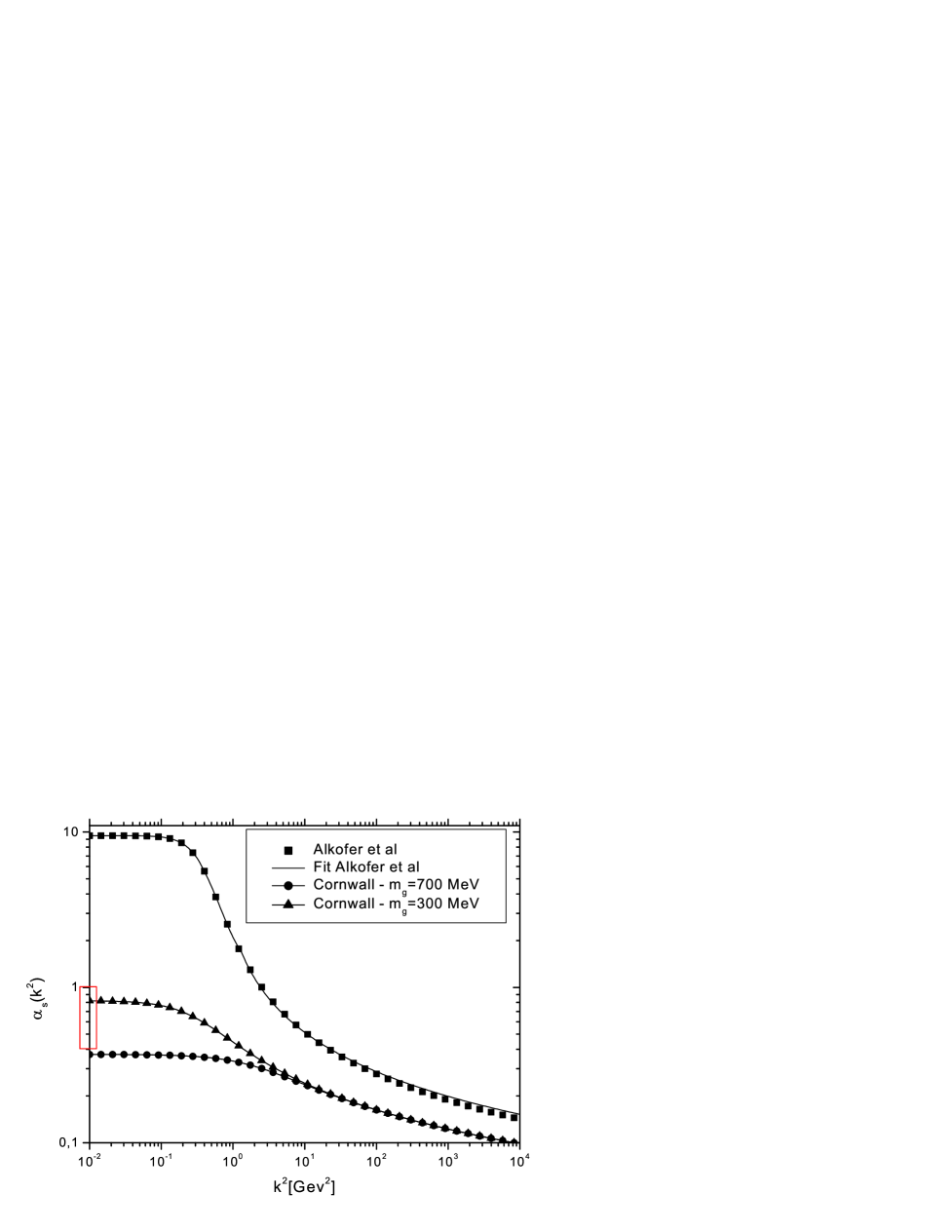
FIG. 1.: Comparison between the running couplings obtained from different approximations in the SDE study. The curves with line + triangle and line + circle delimit the phenomenological range acceptable for the gluon mass ($300$  MeV and $700$  MeV, respectively) with $\Lambda=300$ MeV for the Cornwall’s running coupling. The square points are the numerical data computed by Alkofer et al. and the solid line is our fit Eq.(15). The box in y axis shows the phenomenological range indicated in Eq.(6). We can see that only the running coupling computed by Cornwall is compatible with the phenomenological estimatives of $\alpha_{s}(0)$.

In Fig.(1) we indicate the expected phenomenological range of values for $\alpha_{s}(0)$ and plot the curves for $\alpha_{sC}$ and $\alpha_{sA}$.

It is evident that only the Cornwall’s solution is compatible with the phenomenological data. In the last section we shall comment on possible modifications of this result.

III The nonperturbative coupling and the pion form factor

It is known that the pion form factor, $F_{\pi}(Q^{2})$, is quite dependent on the behavior of $\alpha_{s}$ at small momentum[16]. The asymptotic form factor is predicted by perturbative QCD[16, 21]. It depends on the internal pion dynamics that is parametrized by the quark distribution amplitude of the pion. The QCD expression for the pion form factor is[21]

$$F_{\pi}(Q^{2})=\int_{0}^{1}\!\!dx\!\int_{0}^{1}\!\!dy\, \phi^{*}(y,\tilde{Q}_{y})T_{H}(x,y,Q^{2})$$ (20)

$$\times\phi(x,\tilde{Q}_{x}),$$

where $\tilde{Q}_{x}=\min(x,1-x)Q$ and Q is the 4-momentum in Euclidean space transferred by the photon . The function $\phi(x,\tilde{Q}_{x})$ is the pion wave function, that gives the amplitude for finding the quark or antiquark within the pion carrying the fractional momentum $x$ or $1-x$, respectively. In this work we use the model for the pion distribution amplitude proposed by Chernyak and Zhitnitsky [22]. This wave function was derived from QCD sum rules and it is written as

$$\phi(x,Q)= \frac{f_{\pi}}{2\sqrt{3}}x(1-x)$$ (22)

$$\times\left\{6+\left[30(2x-1)^{2}-6\right]\left(\frac{\alpha_{s}(Q)}{\alpha_{s}(\mu)}\right)^{{\gamma}_{2}}\right\},$$

with $\mu=500\,$ MeV and

$$\gamma_{2}=\frac{50}{99-6n_{f}}.$$ (23)

The other function, $T_{H}(x,y,Q^{2})$, is the hard-scattering amplitude that is obtained by computing the quark-photon scattering diagram as shown in Fig. 2. The lowest-order expression of $T_{H}(x,y,Q^{2})$ is given by (see [23], and references therein)

$$T_{H}(x,y,Q) = \frac{64\pi}{3Q^{2}}\left\{\frac{2}{3}\frac{\alpha_{s}[(1-x)(1-y)Q^{2}]}{(1-x)(1-y)}\right.$$ (25)

$$+\left.\frac{1}{3}\frac{\alpha_{s}(xyQ^{2})}{xy}\right\}$$

To compute the pion form factor using the nonperturbative runningbcouplings proposed by Alkofer et al.[15] and Cornwall Eq.(7), we solved the integrals given by Eq.(20) substituting the quark distribution amplitude written in Eq.(22) and the expression of $T_{H}(x,y,Q^{2})$ (Eq.(25)).

The pion form factor result for the different forms of the QCD coupling in the low momentum regime is shown in Fig.(3). We used for Eq.(7), the lower ($300\,$ MeV) and the upper ($700\,$ MeV) gluon mass values for a fixed $\Lambda=300\,$ MeV. These values defined the shaded area representing the expected range for the pion form factor, $F_{\pi}$.

FIG. 2.: The leading-order diagrams that contribute to the pion form factor. $\phi(x,\tilde{Q}_{x})$ is the pion wave function, that gives the amplitude for finding the quark or antiquark within the pion carrying the fractional momentum $x$ or $1-x$. The photon transfers the momentum $q^{\prime}$ (in Minkowski space), $Q^{2}=-q^{\prime 2}$, for the $q\overline{q}$ pair of total momentum $P$ producing a $q\overline{q}$ pair of final momentum $P^{\prime}$.

In this same figure, we also compare our results with the experimental data (solid line) [24] that was described by the least $\chi^{2}$ fit ($\chi^{2}_{min}=7.96742$) determined in Ref.[25]

$$F^{fit}_{\pi}=\frac{0.46895}{Q^{2}}\left(1-\frac{0.3009}{Q^{2}}\right).$$ (26)

The results, using the running coupling of the Eq.(7), agree very nicely with the experimental data for a gluon mass value close to $700\,$MeV. On the other hand, the calculations with Eq.(15) overestimate $F_{\pi}$ at least by one order of magnitude.

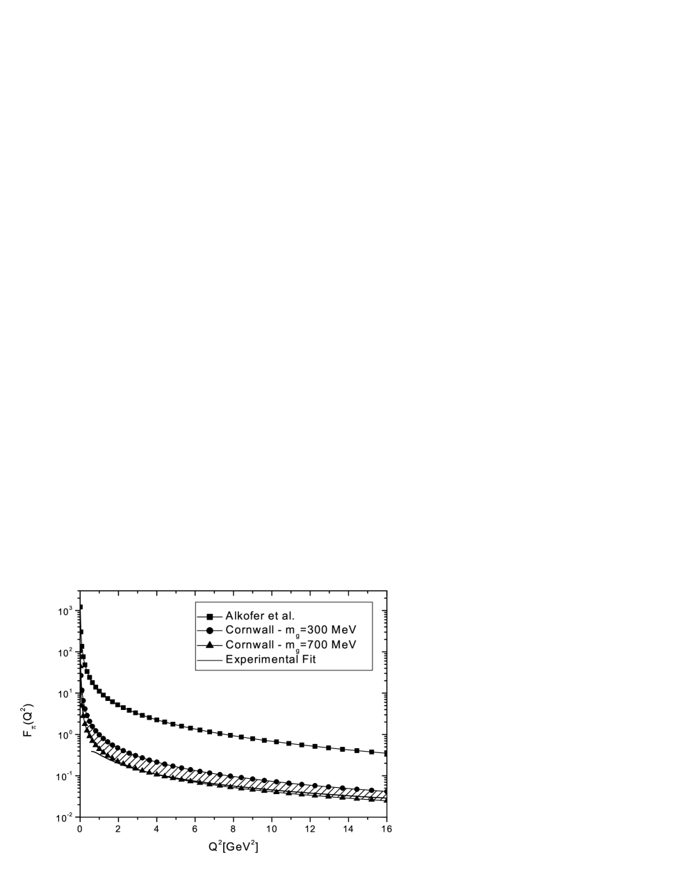
FIG. 3.: Pion form factor computed with the different nonperturbative running coupling constants. The curve composed by line + square is obtained with Eq.(15). The curves that define the shaded area are computed with Eq.(7) for the values of the $m_{g}=300$  (upper curve) and $700$ MeV (lower curve). The solid line is the experimental data fit Eq.(26). There is a nice agreement when $F_{\pi}$ is computed with Cornwall’s running coupling.

IV EFFECTS OF NONPERTURBATIVE PROPAGATORS IN THE $F_{\pi}$ BEHAVIOR

In the previous section we computed $F_{\pi}$ using two distinct forms of the nonperturbative running coupling. We considered that the gluon exchanged by the $q\overline{q}$ pair of Fig.(2) is a perturbative one. However, the SDE solutions at the same time that they give the nonperturbative behavior of the running coupling, they provide nonperturbative expressions for the gluon propagators that at the origin differ drastically from the perturbative propagator.

The large momentum behavior of these nonperturbative propagators coincide with the perturbative one, and, by consistency, we have to use the nonperturbative gluon propagators together with their respective coupling constants, even considering that we are computing the asymptotic pion form factor. So that, it is worth asking whether our previous analysis would be distinct if we change the perturbative gluon propagator by the full one.

In order to introduce this modification, we verify that in Eq.(25) we used the perturbative QCD gluon propagator that, in the Landau gauge, is given by

$$D_{\mu\nu}(q^{2})=\left({\delta}_{\mu\nu}-\frac{q_{\mu}q_{\nu}}{q^{2}}\right)D(q^{2}),\quad D(q^{2})=\frac{1}{q^{2}}.$$ (27)

We can easily factorize $D(q^{2})$ in the Eq.(25), rewritten this last equation as

$$T_{H}(x,y,Q^{2})=\frac{64\pi}{3}\left[\frac{2}{3}\alpha_{s}(K^{2})D(K^{2})+\frac{1}{3}\alpha_{s}(P^{2})D(P^{2})\right],$$ (28)

where $K^{2}=(1-x)(1-y)Q^{2}$ and $P^{2}=xyQ^{2}$.

Let us now consider the two different nonperturbative behaviors of gluon propagators. The first one was obtained by Cornwall[14], and is given by

$$D_{C}(q^{2})=\frac{1}{q^{2}+M_{g}^{2}(q^{2})}.$$ (29)

where $M_{g}(q^{2})$ is the dynamical mass given by Eq.(8). The gluon propagador computed by Alkofer et al.[15], can be fitted by the following expression (${\chi}^{2}=0.016$)

$$D_{A}(q^{2})=\frac{bq^{2}}{q^{4}+a^{4}},$$ (30)

where $a=0.603$ and $b=3.707$.

Once the propagators are given by Eqs.(29,30)then $T_{H}$ (Eq.(28)) will be changed to

$$T_{H}(x,y,Q^{2}) = \frac{64\pi}{3}\left[\frac{2}{3}\alpha_{s}(K^{2})D_{A,C}(K^{2})\right.$$ (32)

$$\left.+\frac{1}{3}\alpha_{s}(P^{2})D_{A,C}(P^{2})\right].$$

We performed the integrations of Eq.(20) numerically, with the amplitude $T_{H}$ given by Eq.(32) and their respective running coupling constant (see Fig.(1)). Our results are shown in Fig.(4).

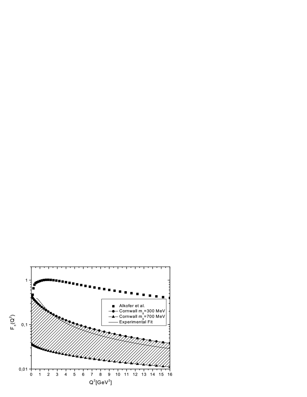
FIG. 4.: Comparison among the experimental curve (solid line) and our results for the pion form factor using the Alkofer’s and Cornwall’s nonperturbative propagators and coupling constants.

If we compare the results of Fig.(4) with the results of the previous section, we can observe a striking attenuation of $F_{\pi}(Q^{2})$ for $Q^{2}\rightarrow 0$. It is also clear that $F_{\pi}(0)$ is finite for both models. This new behavior at low momentum can be understood if we notice that, for $Q^{2}\rightarrow 0$,

$$D_{A}(Q^{2}) \rightarrow 0$$ (33)

$$D_{C}(Q^{2}) \rightarrow \mbox{finite},$$ (34)

in contrast with the divergent perturbative propagator. When we use the nonperturbative information obtained through the SDE with the approximations of Ref.[15], we continue to have a disagreement with the experimental data. In this particular case the pion form factor even go to zero as $Q^{2}\rightarrow 0$.

Obviously we should not consider this region of tranferred momentum because the kernel of Eq.(32) is valid only for large $Q^{2}$, but the disagreement goes through the asymptotic region. On the other hand, the Cornwall’s propagator is still compatible with the experimental data, but now the agreement is in favor of smaller gluon masses.

V Discussion and conclusions

There is an increasing phenomenological evidence for the freezing of the QCD running coupling constant in the infrared region. It is clear that much more work has to be done in order to establish definitively these results. However, it is very satisfying to see that they are not far apart, and are concentrated on a region slightly below $\alpha_{s}\approx 1$.

On the theoretical side there are many studies leading also to this infrared fixed point. Among these we selected the ones derived from the solutions of Schwinger-Dyson equations.

In this work we proposed to test the compatibility between the phenomenological values of $\alpha_{s}(0)$ with the values given by the SDE solutions. This compatibility (or not) can teach us if the approximations used to solve the SDE are realistic or not, and if more data is accumulated we may even be able to discard nonphysical solutions.

We discussed two SDE solutions for the running coupling constant and gluon propagators. One proposed in Ref.[14] and the other in Ref.[15]. These are the only ones consistent with the recent simulations on the lattice of the gluon propagator[13]. These solutions have been obtained in Euclidean space and in pure gauge QCD, i.e. $n_{f}=0$.

The effect of the number of flavors in Cornwall’s solution[14] is not so strong, and it appears in the coefficient $\beta_{0}$ of the coupling constant and in the gluon mass equation increasing the value of the frozen coupling. If a nonzero number of flavors produces any observable effect, this one should act in the same sense for both solutions. Therefore, we do not expect large changes in our results with the inclusion of fermion loops in the SDE solutions, and we can say that the phenomenological data on $\alpha_{s}(0)$ is only compatible with the running coupling determined in Ref.[14].

It is known that different approximations in the same set of SDE produce different results. For example, Atkinson and Bloch solved the same equations of Alkofer et. al using bare truncation and performing an angular averaging of the integrals. In this calculation they obtained $\alpha_{s}(0)=11.47$ [26]. When the angular integrals were performed exactly they found $\alpha_{s}(0)\approx 4.2$ [27]. In all these cases, the incompatibility with phenomenological data is still present. These studies can be improved requiring multiplicative renormalizability of gluon and ghost propagators [28].

It has been claimed that the asymptotic pion form factor is quite dependent on the behavior of $\alpha_{s}$[16]. Therefore, in Section III we computed $F_{\pi}(Q^{2})$ with both SDE solutions. Again, one of the solutions is clearly preferred than the other. Although we followed a traditional calculation performed by several authors, where the form factor was calculated using the nonperturbative running coupling, we commented in Section IV that a consistent treatment is obtained only if the nonperturbative gluon propagators are also taken into account. We modified the expression for the pion form factor including the full gluon propagator. The pion form factor is clearly modified in the infrared in both cases compared to the result of the previous section. It is important to recall that the perturbative QCD expression for $F_{\pi}(Q^{2})$ is not reliable for small $Q^{2}$. However, for large $Q^{2}$ the incompatibility of one of the solutions with the data is apparent.

In summary, the phenomenological data on the low energy behavior of the QCD coupling constant can be used to constrain the solutions of Schwinger-Dyson equations for the coupling constant and gluon propagators. More data is necessary, but the ones already existent indicate that some approximations made in the SDE, leading to a particular value of the running coupling in the infrared region, may not be precise enough to reveal its actual behavior.

REFERENCES

- [1] T. Banks and A. Zaks, Nucl. Phys. B196 (1982) 189.
- [2] G. Grunberg, hep-ph/9911299; see also hep-ph/0009272 and hep-ph/0106070; P. M. Stevenson, Phys. Lett. B331 (1994) 187.
- [3] D. V. Shirkov and I. L. Solovtsov, Phys. Rev. Lett. 79 (1997) 1209; A. V. Nesterenko, Phys. Rev. D62 (2000) 094028; hep-ph/0106305.
- [4] Yu. A. Simonov, Proc. of Schladming Winter School, March 1996, Springer, v.479, p.139 (1997); hep-ph/0109081.
- [5] V. Gribov, preprint Bonn TK 97-08, hep-ph/9708424
- [6] E. Eichten et al., Phys. Rev. Lett. 34 (1975) 369; Phys. Rev. D21 (1980) 203; J. L. Richardson, Phys. Lett.B82 (1979) 272; T. Barnes, F. E. Close and S. Monaghan, Nucl. Phys. B198 (1982) 380.
- [7] S. Godfrey and N. Isgur, Phys. Rev. D32 (1985) 189.
- [8] G. Parisi and R. Petronzio, Phys. Lett. 94B (1980) 51; M. Anselmino and F. Murgia, Phys. Rev. D53 (1996) 5314; A. Mihara and A. A. Natale, Phys. Lett. B482 (2000) 378.
- [9] A. C. Mattingly and P. M. Stevenson, Phys. Rev. Lett. 69 (1992) 1320; Phys. Rev. D49 (1994) 437.
- [10] Yu. L. Dokshitzer and B. R. Webber, Phys. Lett. B352 (1995) 451; Yu. L. Dokshitzer, G. Marchesini and B. R. Webber, Nucl. Phys. B469 (1996) 93.
- [11] C. D. Roberts and A. G. Williams, Prog. Part. Nucl. Phys., 33 477 (1994).
- [12] S. Mandelstam, Phys. Rev. D20 (1979) 3223; N. Brown and M. R. Pennington, Phys. Rev. D38 (1988) 2266; D39 (1989) 2723.
- [13] A. G. Williams et al., hep-ph/0107029; F. D. R. Bonnet et al., hep-lat/0101013; F. D. R. Bonnet et al., Phys. Rev. D62 (2000) 051501; D. B. Leinweber et al. (UKQCD Collaboration) preprint ADP-98-72-T339 (hep-lat/9811027); Phys. Rev. D58 (1998) 031501; C. Bernard, C. Parrinello, and A. Soni, Phys. Rev. D49 (1994) 1585; P. Marenzoni, G. Martinelli, N. Stella, and M. Testa, Phys. Lett. B318 (1993) 511; P. Marenzoni et al., Published in Como Quark Confinement (1994) pp. 210-212 (QCD162:Q83:1994)
- [14] J. M. Cornwall, Phys. Rev. D26 (1982) 1453; J. M. Cornwall and J. Papavassiliou, Phys. Rev. D40 (1989) 3474, D44 (1991) 1285.
- [15] R. Alkofer and L. von Smekal, Phys. Rept. (2001, in press), hep-ph/0007355; L. von Smekal, A. Hauck and R. Alkofer, Ann. Phys. 267 (1998) 1; L. v. Smekal, A. Hauck and R. Alkofer, Phys. Rev. Lett. 79 (1997) 3591.
- [16] C.-R. Ji and F. Amiri, Phys. Rev. D42 (1990) 3764; S. J. Brodsky, C.-R. Ji, A. Pang and D. G. Robertson, Phys. Rev. D57 (1998) 245.
- [17] M. Jezabek, M. Peter and Y. Sumino, Phys. Lett. B428 (1998) 352.
- [18] F. Halzen, G. Krein, and A. A. Natale, Phys. Rev. D47 (1993) 295; M. B. Gay Ducati, F. Halzen, and A. A. Natale, Phys. Rev. D48 (1993) 2324; J. R. Cudell and B. U. Nguyen, Nucl. Phys. B420 (1994) 669; E. V. Gorbar and A. A. Natale, Phys. Rev. D61 (2000) 054012.
- [19] A. M. Badalian and Yu. A. Simonov, Phys. At. Nucl. 60 (1997) 630; A. M. Badalian and V. L. Morgunov, Phys. Rev. D60 (1999) 116008; A. M. Badalian and B. L. G. Bakker, Phys. Rev. D62 (2000) 094031.
- [20] A. M. Badalian and D. S. Kuzmenko, hep-ph/0104097.
- [21] G. P. Lepage and S. J. Brodsky, Phys. Lett. B87 (1979) 359; Phys. Rev. D22 (1980) 2157; S. J. Brodsky, SLAC-PUB-7604, hep-ph/9708345; hep-ph/9710288.
- [22] V. L. Chernyak and I.R. Zhitnitsky, Phys. Rep. 112 (1984) 173;
- [23] E. Braaten and S.-M. Tse, Phys. Rev. D35 (1987) 2255.
- [24] C. J. Bebek et al., Phys. Rev. Lett.37 (1976) 1525; C. J. Bebek et al., Phys. Rev. D17(1978)1693; S. R. Amendolia et al., Nucl. Phys. B 277 (1986) 168.
- [25] Tsung-Wen Yeh, hep-ph/0107192
- [26] D. Atkinson, and J. C. R. Bloch, Phys. Rev. D58 (1998) 094036.
- [27] D. Atkinson, and J. C. R. Bloch, Mod. Phys. Lett. A13 (1998) 1055.
- [28] J. C. R. Bloch, preprint UNITU-THEP-14/01, hep-ph/0106031.