hep-ph/0109214
HIP-2001-51/TH

September 24, 2001

Adiabatic CMB perturbations
in Pre-Big-Bang string cosmology
Kari Enqvist and Martin S. Sloth

Helsinki Institute of Physics

P.O. Box 9, FIN-00014 University of Helsinki, Finland

and

Department of Physics

P.O. Box 9, FIN-00014 University of Helsinki, Finland

We consider the Pre-Big-Bang scenario with a massive axion field which starts to dominate energy density when oscillating in an instanton-induced potential and subsequently reheats the universe as it decays into photons, thus creating adiabatic CMB perturbations. We find that the fluctuations in the axion field can give rise to a nearly flat spectrum of adiabatic perturbations with a spectral tilt $\Delta n$ in the range $-0.1\lesssim\Delta n\lesssim 1$.

1 Introduction

In the Pre-Big-Bang scenario (PBB) [1], which is an attempt to derive the standard Friedman-Robertson-Walker cosmology (FRW) from a fundamental theory of quantum gravity, a FRW universe emerges dynamically after an infinitely long era of dilaton driven super-inflation. This is the so called Pre-Big-Bang era. In the infinite past the universe approaches asymptotically a flat, cold, and empty string perturbative vacuum state. During the PBB era the curvature is growing until it reaches the string scale. At this point the universe enters an intermediate string phase where the curvature stops growing before it ultimately, by some unknown graceful exit mechanism, ends up in the FRW era with a decreasing curvature. The problem of the graceful exit remains largely unsolved, although some promising suggestions has been presented [2].

It has been shown that the amplification of axion quantum fluctuations during the PBB era can lead to initial isocurvature fluctuations with a spectral tilt in an interesting range for the CMB anisotropies [3]. However, the new measurements by the Boomerang balloon flight [4] definitely show that the CMB anisotropies are not of purely isocurvature nature [5]. This presents a very difficult hurdle for the PBB scenario and is the main observational objection against it.

However, as was first noticed in [6] in a different context, a decaying axion field could change the situation dramatically. If the axion field carries power at large scales, then in the FRW era it could dominate the energy density. When it decays into photons, instead of isocurvature fluctuations, one is lead to initial adiabatic density perturbations in the PBB scenario [7].

It has also been noted that a periodic potential for the axion will damp the fluctuations on large scales, avoiding eventual divergences of the large scale axion field fluctuations [6, 8, 9]. The purpose of the present paper is to point out that in the case where the axion, or one of the axions, can decay, there exists a possibility for the PBB scenario to yield adiabatic initial fluctuations with a nearly flat spectrum.

We will assume the generation of the axion field fluctuations during the PBB era and that at some early point during the FRW era the axion acquires a periodic potential due to instanton effects [10]. This happens at some temperature $T_{\Gamma}$ whence the axion mass starts to build up. As soon as the axion mass is of the order of the Hubble rate $m_{a}\simeq 3H$, the axion field starts oscillating and all the long wavelength modes contribute to the total energy density. Given a periodic potential of the type

$$V(\psi)=\frac{1}{2}V_{0}\left(1-\cos\left(\frac{\psi}{\psi_{0}}\right)\right)~{},$$ (1)

and assuming that the axion field is Gaussian distributed with a zero average and a variance $\left<\psi^{2}(\vec{x})\right>$, the average density is given by

$$\rho_{a}=\left<V(\psi(\vec{r}))\right>\approx\frac{1}{2}V_{0}\left(1-e^{-\frac{1}{2}\frac{\left<\psi^{2}(\vec{x})\right>}{\psi_{0}^{2}}}\right)~{}.$$ (2)

Oscillating axions will behave like non-relativistic dust and their energy density will grow compared to the radiation energy density until the axion decays into photons. As we shall argue in section IV, the axions will most likely get to dominate energy density. The fluctuations in the axion energy density will in this way be converted into initial adiabatic fluctuations of radiation.

We presume that we have several axions, one of which decays. In fact, in the effective 4-dimensional theory resulting from compactification of 10-dimensional string theory, one will generally end up with many axion fields. In [10], where the instanton induced axion potential was discussed, one had two axion fields: the string theory axion, which we are interested in here, and the QCD invisible axion. In [11] it was pointed out that the presence of a global $SL(n,\mathbb{R})$ symmetry of the 4-dimensional effective action is a completely general consequence of toroidal compactification from $D+n$ to $D$ dimensions. In a model with $SL(6,\mathbb{R})$ invariance, which is the maximal invariance for compactification from 10 to 4 dimensions, one would have as many as $15$ different axion fields. Cold dark matter (CDM) could for instance be the invisible QCD axion, but it is possible that there are other stable fields with the right properties, such as the moduli fields. We should also like to point out that in models with a $SL(4,\mathbb{R})$ symmetry or higher, there exist regions of the parameter space where the axion with the smallest spectral tilt, which will dominate over the other axions, has a flat or blue spectrum [11].

The paper is organized as follows. In section II we will review how the axion field fluctuations are generated in the Pre-Big-Bang phase [12, 13] and set up our notation. In section III we will estimate the spectral tilt of density fluctuations induced by the decay of the axion in the periodic potential, and in section IV we calculate the life time of the massive axions and discuss the reheat temperature. Section V contains our conclusions.

2 Initial axion field fluctuations

Let us begin our discussion with the following four-dimensional effective tree-level action,

$$S_{eff}=\frac{1}{2\alpha^{\prime}}\int d^{4}x\sqrt{-g}e^{-\phi}\left[\mathcal{R}+\partial_{\mu}\phi\partial^{\mu}\phi-\frac{1}{2}\partial_{\mu}\beta\partial^{\mu}\beta+\mathcal{L}_{matter}\right]~{},$$ (3)

where $\sqrt{\alpha^{\prime}}=\sqrt{8\pi}/M_{s}$ and $M_{s}$ is the string mass. Here $\phi$ and $\beta$ are the universal four-dimensional moduli fields. This action can be derived from 10-dimensional string theory compactified on some 6-dimensional compact internal space. The matter Lagrangian, $\mathcal{L}_{matter}$, is composed of gauge fields and axions, which we assume to be trivial constant fields and not to contribute to the background. In the following we will therefore only consider their quantum fluctuations.

The solution to the equations of motion for the background fields can in the spatially flat case be parameterized as [1, 12, 14, 7]

$$a=a_{s}\left|\frac{\eta}{\eta_{s}}\right|^{(1+\sqrt{3}\cos\zeta)/2}\qquad,\qquad e^{\phi}=e^{\phi_{s}}\left|\frac{\eta}{\eta_{s}}\right|^{\sqrt{3}\cos\zeta}\qquad,\qquad e^{\beta}=e^{\beta_{s}}\left|\frac{\eta}{\eta_{s}}\right|^{\sqrt{3}\sin\zeta}~{}.$$ (4)

Let us split out the part of the matter Lagrangian that contains the axion field $\mathcal{L}_{matter}=\mathcal{L}_{gauge}+\mathcal{L}_{axion}$, where we will assume that the axion Lagrangian has the general form

$$\int d^{4}x\sqrt{-g}e^{-\phi}\mathcal{L}_{axion}\propto\int d\eta d^{3}xa^{2}e^{l\phi}e^{m\beta}(-\sigma^{\prime 2}+(\nabla\sigma)^{2})~{},$$ (5)

where ^′ denotes $\partial/\partial\eta$ and $a$ is the scale factor of the four-dimensional metric $g_{\mu\nu}=a^{2}(\eta)diag(-+++)$. Note that for the model independent axion $m=0$, $l=1$ while for the Ramond-Ramond axion $m\neq 0$, $l=0$.

Let us for simplicity consider a model with two cosmological phases

$$\bar{a}=\bar{a}_{s}\left(\frac{-\eta}{\eta_{s}}\right)^{\alpha}~{}~{},\qquad\eta<-\eta_{s}$$ (6)

$$\bar{a}=\bar{a}_{s}\left(\frac{\eta}{\eta_{s}}\right)~{}~{},\qquad\eta>\eta_{s}$$ (7)

where $\bar{a}$ is the scale factor in the axion frame, defined by

$$\bar{a}\equiv e^{l\phi/2}e^{m\beta/2}a$$ (8)

and $a$ is the scale factor in the string frame. We assume that the dilaton $\phi$ and the moduli $\beta$ are frozen in the post Big Bang era. The axion frame is given by a conformal rescaling of the string frame $g_{\mu\nu}\to\Omega^{2}g_{\mu\nu}$, $\Omega=e^{l\phi/2}e^{m\beta/2}$ [12, 14, 7]. In the axion frame the axions are minimally coupled and the evolution equation for the canonical normalized axion field fluctuation. By matching the PBB solution and its derivative to the FRW post Big Bang solution at $\eta=\eta_{s}$, one finds that during the post Big Bang era [12],

$$\delta\sigma=\frac{C(r)}{\bar{a}\sqrt{2k}}|k\eta_{s}|^{-r-1/2}\sin(k\eta)~{},$$ (9)

where $r=|\alpha-1/2|$ and

$$|C(r)|=\frac{2^{r}\Gamma(r)}{2^{3/2}\Gamma(3/2)}~{}.$$ (10)

Outside the horizon $k\eta<1$, in the post Big Bang era, one can approximate the sine function by its argument and we get

$$\delta\sigma=\frac{C(r)}{\sqrt{2}}e^{-l\phi_{s}/2}e^{-m\beta_{s}/2}\frac{\sqrt{\eta_{s}}}{a_{s}}|k\eta_{s}|^{-r}~{}.$$ (11)

where $a_{s}$ is the scale factor in the string frame at the transition. In the post Big Bang era one assumes $\phi\equiv\phi_{s}$, $\beta\equiv\beta_{s}$. Now let us define the r.m.s. amplitude of the perturbation in a logarithmic $k$ interval $\delta\psi_{k}\equiv k^{3/2}\delta\sigma$ as in [8]. With this definition one obtains

$$\delta\psi_{k}=\frac{C(r)}{\sqrt{2}}e^{-l\phi_{s}/2}e^{-m\beta_{s}/2}M_{s}|k\eta_{s}|^{3/2-r}~{}.$$ (12)

Above we used that $a_{s}\eta_{s}=a_{s}/k_{s}=1/M_{s}$.

Inside the horizon the field fluctuations oscillates in time, and one can read of the r.m.s. amplitude $A$ from Eq. (9)

$$A=\frac{C(r)}{2}\frac{1}{\bar{a}\sqrt{k}}|k\eta_{s}|^{-r-1/2}=\frac{C(r)}{2}\frac{\sqrt{\eta_{s}}}{\bar{a}}|k\eta_{s}|^{-r-1}~{}.$$ (13)

Defining inside the horizon $\delta\psi_{k}\equiv k^{3/2}A$, we get in agreement with [8],

$$\delta\psi_{k}=\frac{C(r)}{2}e^{-l\phi_{s}/2}e^{-m\beta_{s}/2}M_{s}|k\eta_{s}|^{1/2-r}\left(\frac{H(\eta)}{w_{s}(\eta)}\right)~{},$$ (14)

where we used $k_{s}=M_{s}a_{s}$ and $a_{s}/a=H/w_{s}$. The spectral tilt of the axion perturbations is defined as $\gamma\equiv 3/2-r$. If we define $\xi$ by $(\delta\rho_{a})_{k}/\rho_{a}\propto k^{\xi}$, then the spectral tilt $\Delta n$ of the induced curvature perturbations is given by $2\xi$, which in turn depends on $\gamma$ and the ratio $M_{s}/\psi_{0}$, as we will see in section III. For the Ramond-Ramond (R-R) axion $m\neq 0$ unlike for the model independent axion, but in this paper we assume $e^{\beta_{s}}\sim 1$. We will alert the reader whenever the physics is sensitive to this choice.

3 Decaying axion as the origin of initial density perturbations

In this section we will estimate the spectral tilt of the density fluctuations induced by the decay of the axion in the periodic potential. We will assume that when the axion decays, it dominates the energy density and thereby induces adiabatic initial fluctuations for the CMB anisotropies. The periodicity of the potential will damp the fluctuations which are larger than the period of the potential. Due to this effect we are forced to consider the case of a positive tilt spectrum $(\gamma>0)$ and negative tilt spectrum $(\gamma<0)$ separately.

3.1 Negative tilt fluctuations

The relative density fluctuations of the axion field as the potential is turned on is calculated in the Appendix. In case of a negative tilted spectrum we arrive at

$$\frac{\left(\delta\rho_{a}\right)_{k}}{\rho_{a}}\approx\frac{1}{\sqrt{2}}\frac{\delta\psi_{k}}{\psi_{0}}e^{-\frac{1}{2}\int_{k}^{k_{s}}\frac{dk}{k}\frac{\mathcal{P}_{\psi}(k)}{\psi^{2}_{0}}}~{},$$ (15)

which agrees with the result in [8]. Note that in our notation $\mathcal{P}_{\psi}=|\delta\psi|^{2}$. For the model independent axion, which is the case $l=1$, the fluctuations will be completely damped away by the exponential factor. But let us examine the case with $l=0$ more carefully. Let us assume that the spectral tilt $\gamma$ of the axion field fluctuations is negative but very close to zero. In this case there is available one additional degree of freedom, namely the string scale. To evaluate the level of axion density fluctuations we split the integral in Eq. (15) in two:

$$\int_{k_{A}}^{k_{s}}\frac{dk}{k}\frac{\mathcal{P}_{\psi}(k)}{\psi_{0}^{2}}=\int_{k_{A}}^{k_{*}}\frac{dk}{k}\frac{\mathcal{P}_{\psi}(k)}{\psi_{0}^{2}}+\int_{k_{*}}^{k_{s}}\frac{dk}{k}\frac{\mathcal{P}_{\psi}(k)}{\psi_{0}^{2}}~{},$$ (16)

where $k_{A}$ corresponds to the astrophysically interesting comoving scale and $k_{*}$ is the comoving scale that has just entered the horizon when axion starts to oscillate at $\eta=\eta_{*}$. For the last term we get

$$\int_{k_{*}}^{k_{s}}\frac{dk}{k}\frac{\mathcal{P}_{\psi}(k)}{\psi_{0}^{2}}=\frac{M_{s}^{2}}{\psi_{0}^{2}}\int_{k_{*}}^{k_{s}}\frac{dk}{k}\left(\frac{k}{k_{s}}\right)^{2\gamma-2}\left(\frac{H(\eta_{*})}{\omega_{s}(\eta_{*})}\right)^{2}\approx\frac{-1}{2\gamma-2}\frac{M_{s}^{2}}{\psi_{0}^{2}}\left(\frac{k_{*}}{k_{s}}\right)^{2\gamma}~{}$$ (17)

while

$$\int_{k_{A}}^{k_{*}}\frac{dk}{k}\frac{\mathcal{P}_{\psi}(k)}{\psi_{0}^{2}}=\frac{1}{2\gamma}\frac{M_{s}^{2}}{\psi_{0}^{2}}\left[\left(\frac{k_{*}}{k_{s}}\right)^{2\gamma}-\left(\frac{k_{A}}{k_{s}}\right)^{2\gamma}\right]~{}.$$ (18)

In this way we obtain

$$\frac{\left(\delta\rho_{a}\right)_{k_{A}}}{\rho_{a}}=\frac{M_{s}}{\psi_{0}}\left(\frac{k_{A}}{k_{s}}\right)^{\gamma}e^{-\frac{1}{2}\frac{M_{s}^{2}}{\psi_{0}^{2}}\left[\frac{-1}{2(\gamma^{2}-\gamma)}\left(\frac{k_{*}}{k_{s}}\right)^{2\gamma}-\frac{1}{2\gamma}\left(\frac{k_{A}}{k_{s}}\right)^{2\gamma}\right]}~{}.$$ (19)

As we shall see in the next section, we may take $k_{*}/k_{s}\approx 10^{-7}$ within a few orders of magnitude. We did also use $k_{A}/k_{s}\approx 10^{-30}$.

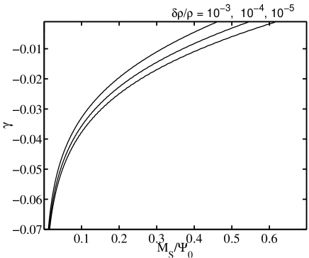
Figure 1: Levels of constant $(\delta\rho_{a})_{k}/\rho_{a}$ as a function of $M_{s}/\psi_{0}$ on the horizontal axis and $\gamma$ on the vertical axis. The three lines correspond to $(\delta\rho_{a})_{k}/\rho_{a}=10^{-3}$, $10^{-4}$, and $10^{-5}$.

In Fig. 1 we show a contour plot of ${\left(\delta\rho_{a}\right)_{k}}/{\rho_{a}}$ as given by Eq. (19) as a function of ${M_{s}}/{\psi_{0}}$ and $\gamma$. We take the lower cut off on the momentum to be $k_{min}\simeq 0$ such that $\rho_{a}=V_{0}/2$ from (Eq. (2)). For ${\left(\delta\rho_{a}\right)_{k}}/{\rho_{a}}=10^{-4}$ we find that the right level of density fluctuations are obtained with $\gamma$ in a reasonable range $-0.04<\gamma<-10^{-5}$ when $0.1<{M_{s}}/{\psi_{0}}<0.6$ (If ${M_{s}}/{\psi_{0}}\gtrsim 1$ then for a negative $\gamma$ the fluctuations are completely damped away for both $l=1$ and $l=0$).

From Fig. 1 we see that if $\psi_{0}$ differs only within a few orders of magnitude from $M_{s}$ we get $\gamma\gtrsim-0.05$ which correspond, as we shall see in the next section, to a bound on the spectral tilt of the adiabatic density fluctuations $\Delta n$ given by $0<\Delta n\lesssim 1$. This is potentially in agreement with experimental bounds [4].

If we require $(\delta\rho_{a})_{k}/\rho_{a}\sim 10^{-4}$ and set $\gamma=-0.01$, we obtain $M_{s}/\psi_{0}\approx 0.4$. It is likely that string theory axions can have a decay constant $\psi_{0}\approx 10^{17}~{}\rm GeV$, which would lead to a present string coupling in the lower limit of the theoretically favoured range $g_{s}\sim 0.1-0.01$. In any case, the possibility of realizing this idea depends very sensitively on the compactification.

When ${M_{s}}/{\psi_{0}}$ is very small, less than $10^{-4}$, the damping switches off. This means that even in this case $\gamma$ can be close to zero with a small but negative spectral tilt $\Delta n=2\xi=2\gamma$ (see next section).

Finally we note that if $e^{\beta_{s}}\neq 1$, the ratio $M_{s}/\psi_{0}$ either increases or decreases, depending on the sign of $m$. It is interesting to note that $m$ can have both signs. In models with an $SL(3,\mathbb{R})$-invariant effective action there are three axions with respectively $m=0$, $m=-\sqrt{3}$, and $m=\sqrt{3}$ [14].

3.2 Positive tilt fluctuations

For the positive tilt case $(\gamma>0)$ one finds the following spectrum (see the Appendix)

$$\frac{\left(\delta\rho_{a}\right)_{k}}{\rho_{a}}\approx\frac{\delta\psi_{k}}{\sqrt{\left<\psi^{2}(\vec{x})\right>}}~{}.$$ (20)

At astrophysical scales we have $k_{A}/k_{s}\simeq 10^{-30}$ and at these scales we want $(\delta\rho_{a})_{k}/\rho_{a}\approx 10^{-4}$. It it is not difficult to see that this is equivalent to requiring

$$\left(\frac{k_{A}}{k_{s}}\right)^{\gamma}\approx 10^{-4}$$ (21)

which implies that the spectral tilt of the axion is $\gamma\simeq 0.13$. This is much closer to flat than what is obtained for adiabatic perturbations induced by the dilaton in the PBB model but still slightly above the observational bounds, as we will see shortly. However, in general we expect a combination of isocurvature and adiabatic perturbations, which can change the bounds somewhat.

The approximation used in the positive tilt case breaks down when $(k_{A}/k_{s})^{\gamma}\sim 1$, i.e. when $\gamma\sim 0$. Therefore we can not exclude that a more careful analysis could show that for $\gamma$ almost zero but positive one obtains also the right level of density perturbations.

3.3 Spectral tilt of the CMB anisotropies

Let us now estimate the spectral index of the CMB fluctuations corresponding to a slightly negative or positive value for the axion tilt $\gamma$. We define $\Phi_{k}$ as in [15]

$$k^{-3/2}\frac{(\delta\rho)_{k}}{\rho}\equiv\delta_{k}=-\frac{2}{3}\left(\frac{k}{aH}\right)^{2}\Phi_{k}$$ (22)

whence one can calculate the relation of $\Phi_{k}$ to the curvature fluctuation $\mathcal{R}_{k}$

$$\Phi_{k}=-\frac{3+3w}{5+3w}\mathcal{R}_{k}~{},$$ (23)

where $w=P/\rho$. Thus during radiation domination $w=1/3$.

The spectral index $n$ of adiabatic (curvature) fluctuations is defined by

$$\mathcal{P}_{\mathcal{R}}(k)\propto k^{n-1}$$ (24)

evaluated at the horizon entry; $n=1$ corresponds to the scale invariant Harrison-Zel’dovich spectrum. Given that

$$\frac{(\delta\rho)_{k}}{\rho}\propto k^{\xi}\qquad\Rightarrow\delta_{k}=k^{\xi-3/2}$$ (25)

we get $n=2\xi+1$ so that the spectral tilt $\Delta n\equiv n-1$ is given by

$$\Delta n\equiv 2\xi$$ (26)

For a positive tilt with $\xi=\gamma\sim 0.13$ we would get a spectral tilt $\Delta n=0.26$. The resulting index is slightly above $n=1.06$ which is the upper limit given by Boomerang [4], although one should note that an uncorrelated isocurvature component has the effect of raising the best fit for the adiabatic spectral index [16]. For a small negative tilt $\gamma>-0.05$ the damping factor in eq.(15) implies that this gives rise to a slightly positive tilted (blue) spectrum of density fluctuations $0.3\lesssim\Delta n\lesssim 1$. Only if the ratio $M_{s}/\psi_{0}$ is very small, such that the damping switches off, it is possible to get a negative tilt. This result is obtained assuming that the axion density fluctuations are approximately unchanged by the coherent oscillations and the subsequent decays. However if the amplitude of the axion field fluctuations looses some magnitude as the axions become non-relativistic it will make the spectrum, that fits the amplitude at the COBE scale, much more flat. We will return to this issue with a more detailed analysis in a later paper.

Since the axion potential is highly non-linear, it is not trivial to solve the perturbation equation mode-by-mode and to compute the perturbations after the onset of the potential. For a quadratic axion potential, valid for small field values, one finds that at low frequencies the spectral tilt of the energy density is unchanged after the onset of the potential [13, 8]. However, the spectrum of a massive scalar field changes for modes that become non-relativistic outside the horizon [17, 13]. Therefore it would be important to study the evolution of the field fluctuations on superhorizon scales after the potential is generated and the axion mass has become larger than the Hubble rate. In this way one could check whether the evolution of the fluctuations on superhorizon scales affects the spectral tilt. In the present paper we have instead followed an approach similar to that suggested in [8, 9].

To understand what happens after the potential is turned on, we divide the field $\psi$ in its large scale component, which at scales $l=k^{-1}$ behaves as a constant classical field $\psi_{c}(l^{-1})$, and its short wave length part $\delta\psi$ corresponding to momenta $k\geq l^{-1}$,

$$\psi=\psi_{c}(l^{-1})+\delta\psi$$ (27)

where

$$\psi_{c}(l^{-1})=\psi_{c}+\tilde{\psi}(l^{-1})~{}.$$ (28)

Here $\psi_{c}(l^{-1})$ includes the classical scale independent field $\psi_{c}$ together with a contribution $\tilde{\psi}(l^{-1})$ from all the fluctuations with momenta smaller than $k$. The dispersion of the long-wave perturbations $\tilde{\sigma}_{k}=\sqrt{\sigma^{2}-\sigma_{k}^{2}}$, is given by

$$\tilde{\sigma}^{2}_{k}=\int_{k_{min}}^{k}d\ln k\left|\delta\psi(k)\right|^{2}~{}.$$ (29)

If $\tilde{\sigma}_{k}$ is comparable to $\psi_{c}$ then $\psi_{c}(l^{-1})$ will indeed depend on $x$.

It is natural to assume that when the potential is turned on, the field will oscillate a few times in the potential. As the amplitude of the coherent oscillations decreases, the potential effectively becomes quadratic. This is equivalent to the statement that the axions will behave like non-relativistic matter when they oscillate coherently in the potential. If $\psi_{c}(l^{-1})$ does not change considerably at a distance $l\sim k^{-1}$ we find [9]

$$\frac{\rho_{\psi}(k)}{\rho_{\psi}}\sim\frac{\delta V\left(\psi\left(k\right)\right)}{V\left(\psi\right)}\sim\frac{\delta\psi(k)}{\psi}$$ (30)

where $\psi$ can be identified with $\psi_{c}(l^{-1})$. This is valid if $\psi_{c}(l^{-1})$ is larger than the short-wave length dispersion $\sigma_{k}$. In the opposite limit we would get

$$\frac{\rho_{\psi}(k)}{\left<\rho_{\psi}\right>}\sim\frac{\delta V\left(\psi\left(k\right)\right)}{\left<V\left(\psi\right)\right>}\sim\frac{\left(\delta\psi(k)\right)^{2}}{\left<\right.\left(\delta\psi(k)\right)^{2}\left.\right>}~{}.$$ (31)

Since $\psi_{c}(l^{-1})$ evolves in the same way as $\delta\psi(k)$ and $\left(\delta\psi(k)\right)^{2}$ evolves in the same way as $\left<\right.\left(\delta\psi(k)\right)^{2}\left.\right>$, we note that the ratios in eq.(30) and eq.(31) remains fixed up to some scale-independent factor that does not destroy the scale invariance of the spectrum [18]. This is consistent with the calculation of [13, 8] where it was shown for a quadratic potential that when the field becomes non-relativistic the energy spectrum does not change on large scales (up to a scale-independent factor).

In the case $\delta\rho_{\psi}\sim\delta\psi(k)$ in eq.(30) the density fluctuations will be gaussian, while in the case of eq.(31) the density fluctuations will have a $\chi^{2}$-distributed non-gaussian nature [18]. A $\chi^{2}$ perturbation is ruled out by observations [19]. Since large field fluctuations are topologically cut off at the onset of the potential, it seems likely that one will obtain non-gaussian fluctuations unless the spectrum is very close to flat. Since the evolution of $\delta\psi(k)$ is non linear from the moment when the potential is turned on until the potential can be treated as quadratic, a study of the extend of the non-gaussianity of the density perturbations is beyond the scope of this paper.

4 Reheat temperature and entropy production

Let us now check that the axions have a chance of dominating the energy density, as was assumed in the previous section. To estimate the life time of the massive axions, we parameterize the interaction between the axion and the gauge fields as

$$(\psi/M^{\prime})F\tilde{F}~{},$$ (32)

where $M^{\prime}\sim\pi^{2}\psi_{0}$ generally depends on the compactification [6, 10]. A typical axion lifetime is [6, 10]

$$\tau_{a}\approx M^{\prime 2}/m_{a}^{3}~{},$$ (33)

where the axion mass $m_{a}$ is given by

$$m_{a}\approx 10\frac{\Lambda^{3}}{M_{p}M^{\prime}}~{}.$$ (34)

With $M^{\prime}\sim 10^{18}~{}\rm GeV$ we get $m_{a}=10^{6}~{}\rm GeV$ and thus $k_{*}/k_{s}\sim 10^{-7}$ as claimed in the previous section. Like in [6] we will assume that $\Lambda\approx 10^{14}~{}\rm GeV$. Defining $R\equiv M^{\prime}/M_{p}$ one finds that

$$\tau_{a}\approx 10^{-3}R^{5}\frac{M_{p}^{8}}{\Lambda^{9}}\approx R^{5}\cdot 10^{23}~{}\rm GeV^{-1}\approx\mathnormal{R}^{5}\cdot 10^{-2}~{}\mathrm{sec}~{}.$$ (35)

The average energy density in the non-relativistic part of the axion field after the potential is turned on reads

$$\rho_{a}=\left<V(\psi(\vec{r}))\right>\approx\frac{1}{2}V_{0}~{},$$ (36)

which implies that the relative energy density of the axions is

$$\Omega_{a}=\frac{\rho_{a}}{\rho_{c}}=\frac{4\pi}{3}\frac{V_{0}}{M_{p}^{2}H^{2}}~{}.$$ (37)

To evaluate $\Omega_{a}$ at the time the potential is turned on, we use the fact that at this time the Hubble paremeter $H$ has the same order of magnitude as the axion mass. Typically we can also take [6, 10]

$$V_{0}\approx\frac{\Lambda^{6}}{M_{p}^{2}}$$ (38)

so that we obtain

$$\Omega_{a}\approx 4\pi\frac{\Lambda^{6}}{M_{p}^{4}m_{a}^{2}}\simeq 10^{-1}\frac{M^{\prime 2}}{M_{p}^{2}}=10^{-1}R^{2}~{},$$ (39)

in agreement with [20]. Thus the axions do not dominate energy density at this point. This works only if we assume that the axion fluctuations do not have a large negative tilt, which would amplify small momentum mode fluctuations as they enter the horizon and possibly make the axion dominate energy density before the axion mass is turned on. If $\gamma>-0.05$ as in Fig.1 there is no problem.

The axion behaves as non-relativistic dust and soon starts to dominate the energy density. Let us evaluate the reheat temperature $T_{RH}$ as the axion decays into photons. Since $H\approx 1.66g_{*}^{1/2}T^{2}/M_{p}$ so that $H^{2}(t=\tau)\approx\frac{1}{4}\tau^{-2}\approx 2.8g_{*}T_{RH}^{4}/M_{p}^{2}$ which implies that

$$T_{RH}=0.55g_{*}^{-1/4}\frac{M_{p}^{1/2}}{\tau^{1/2}}$$ (40)

we obtain

$$T_{RH}\sim R^{-5/2}10^{-2}~{}\rm GeV~{}.$$ (41)

In [6] the entropy production associated with the decay of the axion was calculated as

$$\Delta s\simeq 10^{15}\left(\frac{A_{0}}{M^{\prime}}\right)^{2}\left(\frac{\Lambda}{10^{14}~{}\rm GeV}\right)^{-3}R^{4}\Omega_{r}^{-3/4}$$ (42)

where $A_{0}\sim M^{\prime}/\pi$ is the initial displacement of the axion VEV and $\Omega_{r}\equiv N_{r}/N_{tot}$. $N_{r}$ is the number of degrees of freedom in spin 0 and 1 fields charged under the gauge groups of the observable sector. $N_{tot}$ is the total number of degrees of freedom in spin 0, 1, and 2. We expect $0.01\lesssim\Omega_{r}\lesssim 1$. By tuning the parameters slightly, it is possible to obtain a reasonable amount of entropy production of 8 to 10 orders of magnitude in order to dilute dangerous relics [6].

If we define $T_{*}$ as the temperature of the universe when $m_{a}=3H$, we find

$$T_{*}\approx\sqrt{\frac{m_{a}M_{p}}{5g_{*}^{1/2}}}\approx\sqrt{\frac{\Lambda^{3}}{RM_{p}}}\sim R^{-1/2}10^{11}~{}\rm GeV~{}.$$ (43)

We denote the temperature as the axions decay by $T_{D}$. Noting that $T_{D}<T_{RH}$ and $T_{*}>10^{11}~{}\rm GeV$ we can conclude that indeed the universe will become matter dominated soon after the axion mass is turned on.

Let us choose as a typical example $R\sim 10^{-2}$. In this case $T_{RH}=10^{3}~{}\rm GeV$, but one needs to tune the other parameters in order to have enough entropy production to dilute dangerous relics. If $R\sim 1$, then one is about to get in trouble with a too low reheat temperature $T_{RH}=10~{}\rm MeV$, but there is plenty of entropy production.

If baryogenesis is due to the decay of an Affleck-Dine (AD) condensate, the AD condensate must not dominate energy density as the axion decays. However it is possible that the decay of the AD condensate produces a much too high baryon asymmetry and that the late decay of the axion dilutes this to the level $n_{B}/s\sim(4-7)\times 10^{-11}$ [6].

5 Conclusion

We have shown that if one of the PBB axions decay to photons, it is possible to get an adiabatic initial fluctuation for the CMB anisotropies. Moreover, the considerations presented here seem to point towards a small tilt, i.e. a nearly flat spectrum, although the tilt of the initial adiabatic fluctuations may depend on the axion oscillation and decay dynamics; here we have assumed that the fluctuations are frozen during this time.

Our approach here is slightly different from [6], where it was suggested that a negative tilt would make the axions dominate energy density as the large wavelength modes enters the horizon, and that the large fluctuations would be sufficiently damped by the periodic potential. We have assumed that the spectrum is nearly flat and the axions gets to dominate energy density because they behave like non-relativistic dust when oscillating in the harmonic potential. The fluctuations are damped, but the relative magnitude of the string scale compared to the decay constant plays a crucial role. In the positive tilt case we found the additional possibility that the size of the tilt determines the relative level of axion energy density fluctuations.

Since generically there is several string theory axions in the type of models which we have discussed, it is possible that the other axions, which are not expected to have decayed within the present age of the universe, will carry isocurvature fluctuations but with an amplitude smaller than the adiabatic fluctuations. It seems thus viable that the scenario we have presented here will generally lead to a mixture of adiabatic and isocurvature fluctuations, with a dominating adiabatic component. Hence it appears that the Pre-Big-Bang model does not necessaryly produce only initial isocurvature fluctuations and can remain a potential candidate for explaining the observed CMB data. Note also that the intermediate matter dominated phase could give a kink in the gravitational wave spectrum, which if observable would be an interesting feature.

A decaying axion may also be benefical from the point of view of dangerous relics, which the entropy production associated with the decay could dilute. A generic feature of this scenario is a late reheat temperature which however is within the required bound from Big Bang Nucleosynthesis.

We have kept our discussion general and did not constrain ourselves to any specific compactification scheme of the 10-dimensional string theory. It would however be important to investigate whether one can construct a specific model with the desired features.

Acknowledgements

We would like to thank Riccardo Sturani for his interesting comments about the gravitational wave spectrum. Martin S. Sloth would also like to thank Fawad Hassan and Jussi Väliviita for the inspiration from many discussions and especially Jussi for also lending out his matlab skills. K.E. partly supported by the Academy of Finland under the contracts 35224 and 47213. M.S.S. partly supported by the TMR network Finite temperature phase transitions in particle physics, EU contract no. FMRX-CT97-0122.

Appendix

Damping due to the periodic nature of the potential

Here we calculate the damping of the fluctuations in the axion energy density. We present a simple intuitive argument.

Fluctuations in the axion energy density at scales $l\sim k^{-1}$ can be computed by using the following relation

$$\int_{0}^{\infty}d\ln k\left(\delta\rho_{a}^{2}\right)_{k}\frac{\sin(kr)}{kr}=\left<V\left(\frac{\psi(\vec{x})}{\psi_{0}}\right)V\left(\frac{\psi(\vec{x}+\vec{r})}{\psi_{0}}\right)\right>-\left<V\left(\frac{\psi(\vec{x})}{\psi_{0}}\right)\right>^{2}~{}.$$ (44)

By assuming that the fluctuatons in $\psi$ are Gaussian such that any connected correlation function of order higher than two vanish, we get in agreement with [8]

$$\int_{0}^{\infty}d\ln k\left(\delta\rho_{a}^{2}\right)_{k}\frac{\sin(kr)}{kr}=\frac{1}{4}V_{0}^{2}e^{-\frac{\left<\psi^{2}(\vec{x})\right>}{\psi_{0}^{2}}}\left[\cosh\left(\frac{\left<\psi(\vec{x})\psi(\vec{x}+\vec{r})\right>}{\psi^{2}_{0}}\right)-1\right]~{}.$$ (45)

To evaluate $(\delta\rho_{a})_{k}$, we need to consider two limiting cases

$$\int_{0}^{1/l}d\ln k\frac{\mathcal{P}_{\psi}(k)}{\psi^{2}_{0}}>>\int_{1/l}^{\infty}d\ln k\frac{\mathcal{P}_{\psi}(k)}{\psi^{2}_{0}}$$ (46)

and

$$\int_{0}^{1/l}d\ln k\frac{\mathcal{P}_{\psi}(k)}{\psi^{2}_{0}}<<\int_{1/l}^{\infty}d\ln k\frac{\mathcal{P}_{\psi}(k)}{\psi^{2}_{0}}$$ (47)

which respectively are typical for a negative and a positive tilted spectrum.

Let us consider the first case. By integrating Eq. (45) on both sides by $\int d^{3}x\int_{|\vec{k}|<1/l}d^{3}ke^{i\vec{x}\cdot\vec{k}}$, we obtain

$$\int_{0}^{1/l}d\ln k\left(\delta\rho_{a}^{2}\right)_{k}=\frac{1}{4}V_{0}^{2}e^{-\frac{\left<\psi^{2}(\vec{x})\right>}{\psi_{0}^{2}}}~{}~{}~{}~{}~{}~{}~{}~{}~{}~{}~{}~{}~{}~{}~{}~{}~{}~{}~{}~{}~{}~{}~{}~{}~{}~{}~{}~{}~{}~{}~{}~{}~{}~{}~{}~{}~{}~{}~{}~{}~{}~{}~{}~{}~{}~{}~{}~{}~{}~{}~{}~{}~{}~{}~{}~{}~{}~{}~{}~{}~{}~{}~{}~{}$$

$$\times\sum_{n=1}^{\infty}\frac{1}{2n!}\int\frac{d^{3}k_{1}}{4\pi k_{1}^{3}}\frac{\mathcal{P}_{\psi}(k_{1})}{\psi^{2}_{0}}\cdots\int\frac{d^{3}k_{2n}}{4\pi k_{2n}^{3}}\frac{\mathcal{P}_{\psi}(k_{2n})}{\psi^{2}_{0}}\int_{|\vec{k}|<1/l}d^{3}k\delta\left(\sum_{i=1}^{2n}\vec{k}_{i}-\vec{k}\right)~{}.$$ (48)

We first note that

$$\int_{|\vec{k}|<1/l}d^{3}k\delta\left(\sum_{i=1}^{2n}\vec{k}_{i}-\vec{k}\right)=\left\{\begin{array}[]{ccc}0&if&|\sum_{i=1}^{2n}\vec{k}_{i}|>1/l\\ 1&if&|\sum_{i=1}^{2n}\vec{k}_{i}|<1/l\end{array}\right.$$ (49)

and assuming

$$\int_{0}^{1/l}d\ln k\frac{\mathcal{P}_{\psi}(k)}{\psi^{2}_{0}}>>\int_{1/l}^{\infty}d\ln k\frac{\mathcal{P}_{\psi}(k)}{\psi^{2}_{0}}>0~{},$$ (50)

we arrive at the following crude approximation

$$\int_{0}^{1/l}d\ln k\left(\delta\rho_{a}^{2}\right)_{k}\simeq\frac{1}{4}V_{0}^{2}e^{-\frac{\left<\psi^{2}(\vec{x})\right>}{\psi_{0}^{2}}}\sum_{n=1}^{\infty}\frac{1}{2n!}\int_{0}^{1/l}\frac{dk_{1}}{k_{1}}\frac{\mathcal{P}_{\psi}(k_{1})}{\psi^{2}_{0}}\cdots\int_{0}^{1/l}\frac{dk_{2n}}{k_{2n}}\frac{\mathcal{P}_{\psi}(k_{2n})}{\psi^{2}_{0}}~{}.$$ (51)

Instead of $0$ and $\infty$ as lower and upper limit for $k$, we introduce the more physical upper and lower limits $k_{s}$ and $k_{min}$. Then we get

$$\int_{k_{min}}^{1/l}d\ln k\left(\delta\rho_{a}^{2}\right)_{k}\approx\frac{1}{8}V_{0}^{2}e^{-\int_{1/l}^{k_{s}}\frac{dk}{k}\frac{\mathcal{P}_{\psi}(k)}{\psi^{2}_{0}}}$$ (52)

which agrees with the result in [6]. If we use $\left<\rho_{a}\right>=\frac{1}{2}V_{0}$ we obtain

$$\frac{\left(\delta\rho_{a}\right)_{k}}{\rho_{a}}\approx\frac{1}{\sqrt{2}}\frac{\delta\psi_{k}}{\psi_{0}}e^{-\frac{1}{2}\int_{k}^{k_{s}}\frac{dk}{k}\frac{\mathcal{P}_{\psi}(k)}{\psi^{2}_{0}}}~{}.$$ (53)

Hence in the negative tilt case the fluctuations are exponentially damped, as discussed in section (3.1).

In the positive tilt case, we do not have the control of the integral in Eq. (A0.Ex1) but calculate instead

$$\int_{1/l}^{\infty}d\ln k\left(\delta\rho_{a}^{2}\right)_{k}=\frac{1}{4}V_{0}^{2}e^{-\frac{\left<\psi^{2}(\vec{x})\right>}{\psi_{0}^{2}}}~{}~{}~{}~{}~{}~{}~{}~{}~{}~{}~{}~{}~{}~{}~{}~{}~{}~{}~{}~{}~{}~{}~{}~{}~{}~{}~{}~{}~{}~{}~{}~{}~{}~{}~{}~{}~{}~{}~{}~{}~{}~{}~{}~{}~{}~{}~{}~{}~{}~{}~{}~{}~{}~{}~{}~{}~{}~{}~{}$$

$$\times\sum_{n=1}^{\infty}\frac{1}{2n!}\int\frac{d^{3}k_{1}}{4\pi k_{1}^{3}}\frac{\mathcal{P}_{\psi}(k_{1})}{\psi^{2}_{0}}\cdots\int\frac{d^{3}k_{2n}}{4\pi k_{2n}^{3}}\frac{\mathcal{P}_{\psi}(k_{2n})}{\psi^{2}_{0}}\int_{|\vec{k}|>1/l}d^{3}k\delta\left(\sum_{i=1}^{2n}\vec{k}_{i}-\vec{k}\right)~{}.$$ (54)

In this case we use

$$\int_{|\vec{k}|>1/l}d^{3}k\delta\left(\sum_{i=1}^{2n}\vec{k}_{i}-\vec{k}\right)=\left\{\begin{array}[]{ccc}0&if&|\sum_{i=1}^{2n}\vec{k}_{i}|<1/l\\ 1&if&|\sum_{i=1}^{2n}\vec{k}_{i}|>1/l\end{array}\right.$$ (55)

which motivates the following approximation

$$\int_{1/l}^{\infty}d\ln k\left(\delta\rho_{a}^{2}\right)_{k}=\frac{1}{4}V_{0}^{2}e^{-\frac{\left<\psi^{2}(\vec{x})\right>}{\psi_{0}^{2}}}~{}~{}~{}~{}~{}~{}~{}~{}~{}~{}~{}~{}~{}~{}~{}~{}~{}~{}~{}~{}~{}~{}~{}~{}~{}~{}~{}~{}~{}~{}~{}~{}~{}~{}~{}~{}~{}~{}~{}~{}~{}~{}~{}~{}~{}~{}~{}~{}~{}~{}~{}~{}~{}~{}~{}~{}~{}~{}~{}~{}~{}~{}~{}$$ (56)

$$\times\sum_{n=1}^{\infty}\frac{1}{2n!}\int_{0}^{\infty}\frac{dk_{1}}{k_{1}}\frac{\mathcal{P}_{\psi}(k_{1})}{\psi^{2}_{0}}\cdots\int_{0}^{\infty}\frac{dk_{2n-1}}{k_{2n-1}}\frac{\mathcal{P}_{\psi}(k_{2n-1})}{\psi^{2}_{0}}\int_{1/l}^{\infty}\frac{dk_{2n}}{k_{2n}}\frac{\mathcal{P}_{\psi}(k_{2n})}{\psi^{2}_{0}}~{}.$$ (57)

Again we introduce the more physical upper and lower limits $k_{s}$ and $k_{min}$ and obtain

$$\frac{\left(\delta\rho_{a}^{2}\right)_{k}}{\rho_{a}^{2}}\approx\frac{1}{2}\frac{\delta\psi_{k}^{2}}{\left<\psi^{2}(\vec{x})\right>}\left(\frac{1-e^{-\frac{\left<\psi^{2}(\vec{x})\right>}{\psi_{0}^{2}}}}{1-e^{-\frac{1}{2}\frac{\left<\psi^{2}(\vec{x})\right>}{\psi_{0}^{2}}}}\right)^{2}\approx\frac{\delta\psi_{k}^{2}}{\left<\psi^{2}(\vec{x})\right>}~{}.$$ (58)

As discussed in section (3.2), we find for the positive tilt case that the fluctuations are not damped.

References

- [1] G. Veneziano, Phys. Lett. B265, 287 (1991); M. Gasperini and G. Veneziano, Astropart. Phys. 1, 317 (1993); Mod. Phys. Lett. A8, 3701 (1993).
- [2] M. Gasperini, M. Maggiore, and G. Veneziano, Nucl. Phys. B494, 315 (1997); R. Brustein and R. Madden, Phys. Lett. B410, 110 (1997); Phys. Rev. D57, 712 (1998); S. Foffa, M. Maggiore, and R. Sturani, Nucl. Phys. B552, 395 (1999); C. Cartier, E. J. Copeland, and R. Madden, J. High Energy Phys. 01, 035 (2000).
- [3] R. Durrer, M. Gasperini, M. Sakellariadou, and G. Veneziano, Phys. Lett. B436, 66 (1998); Phys. Rev. D59, 043511 (1999). A. Melchiorri, F. Vernizzi, R. Durrer, and G. Veneziano, Phys. Rev. Lett. 83, 4464 (1999). F. Vernizzi, A. Melchiorri, and R. Durrer, Phys. Rev. D63, 063501 (2001).
- [4] P. de Bernardis et. al.: astro-ph/0105296.
- [5] K. Enqvist, H. Kurki-Suonio, and J. Väliviita, astro-ph/0108422.
- [6] A. Buonanno, M. Lemoine, and K. A. Olive, Phys. Rev. D62, 083513 (2000).
- [7] E.J. Copeland, J. E. Lidsey, and D. Wands, Phys. Rep. 337, 343 (2000).
- [8] R. Brustein and M. Hadad, Phys. Lett. B442, 74 (1998).
- [9] A. D. Linde, Phys. Lett. B158, 375 (1985); L. A. Kofman, Phys. Lett. B173, 400 (1986); L. A. Kofman and A. D. Linde, Nucl. Phys. B282, 555 (1987).
- [10] K. Choi and J. E. Kim, Phys. Lett. B165, 71 (1985).
- [11] H. A. Bridgman and D. Wands, Phys. Rev. D 61, 123514 (2000).
- [12] E.J. Copeland, A. Lahri, and D. Wands, Phys. Rev. D50, 4868 (1994); E.J. Copeland, J. E. Lidsey, and D. Wands, Phys. Rev. D56, 874 (1997).
- [13] R. Brustein and M. Hadad, Phys. Rev. D57, 725 (1998).
- [14] E.J. Copeland, J. E. Lidsey, and D. Wands, Phys. Lett. B443, 97 (1998).
- [15] A. R. Liddle, D. H. Lyth: Cosmological inflation and large-scale structure Cambridge university press 2000.
- [16] K. Enqvist, H. Kurki-Suonio, and J. Väliviita, Phys. Rev. D62, 103003 (2000).
- [17] M. Gasperini and G. Veneziano, Phys. Rev. D59, 043503 (1999).
- [18] D. H. Lyth and D. Wands, hep-ph/0110002.
- [19] H. A. Feldman, J. A: Frieman, J. N. Fry, and R. Scocciarro, Phys. Rev. Lett. 86, 1434 (2001),
- [20] T. Banks and M. Dine, Nucl. Phys. B505, 445 (1997).