$\Theta$ vacua states in heavy ion collisions in presence of dissipation and noise

Abstract

We have studied possible formation of $\Theta$ vacua states in heavy ion collisions. Random phases of the chiral fields were evolved in a finite temperature potential, incorporating the breaking of $U_{A}(1)$ symmetry. Initial random phases very quickly settle into oscillation around the values dictated by the potential. The simulation study indicate that an initial $\Theta$=0 state do not evolve into a $\Theta$ $\neq$ 0 state. However, an initial $\Theta$ $\neq$ 0 state, if formed in heavy ion collision, can survive, as a coherent superposition of a number of modes.

I Introduction

QCD in the chiral limit ($m_{u}=m_{d}=m_{s}=0$) possesses a $U_{A}(1)$ symmetry. Spontaneous breaking of the symmetry requires a neutral pseudoscalar Goldstone boson with mass less than $\sqrt{3}m_{\pi}$, in addition to pion itself. However no such Goldstone boson is seen in nature. The problem was resolved by the discovery of non perturbative effects that violates the extra $U_{A}(1)$ symmetry. ’t Hooft showed that because of the instanton solutions of the Yang-Mills theory, the axial anomaly has nonzero physical effects, and there is not really a U(1) [2]. Term containing the so called vacuum angle ($\Theta$) which breaks $P$ and $CP$ symmetry can be added to the Lagrangian. QCD requires very small $\Theta\sim 10^{-9}$, which explain the apparent $P$ and $CP$ symmetries in strong interaction Dynamical breaking of the $U_{A}(1)$ symmetry is also obtained in large $N$ (color) limit of the SU(N) gauge theory [3, 4, 5]. In this approach the dominant fluctuations are not semi classical but of quantum nature.

Recently Kharzeev, Pisarski and Tytgat [6] and Kharzeev and Pisarski [7] argued That, in heavy ion collisions, a non trivial $\Theta$ vacua state may be created. In the limit of large number of colors, the axial $U_{A}(1)$ symmetry of massless quarks may be restored at the deconfining phase transition. As the system rolls back to confining phase, it may settles into a metastable state with non- trivial $\Theta$. The idea is similar to the formation of disoriented chiral condensate (DCC) [8]. In DCC, space-time region is created, where the chiral condensate points in a direction, different from the ground state direction. Similarly, in a $\Theta$ vacua states, space-time region with non-trivial $\Theta$ is created. $\Theta$ vacua state being P and CP odd, such a state, if produced in heavy ion collisions, may have some interesting signals, e.g. decay of $\eta$ into two pions, which is strongly forbidden in our world.

After the suggestion of Kharzeev and co-workers [6, 7], several authors have looked into various aspects of nontrivial $\Theta$ vacua state, that may be formed in heavy ion collisions. [9, 10, 11, 12]. Buckley et al. [11, 12] numerically simulated the formation of $\Theta$ vacua states, using the effective Lagrangian of Halperin and Zhitnitsky [15]. They assumed quenchlike scenario, rapid expansion of the fireball leave behind an effectively zero temperature region, interior of which is isolated from the true vacuum. Starting from an initial nonequilibrium state, they studied the evolution of phases of the chiral field, in a dissipative environment. They saw formation of nonzero $\Theta$ vacuum within a time scale of $10^{-23}$ sec. They choose to ignore the fluctuation-dissipation theorem, which require the dissipation to be associated with fluctuations. Recently we have performed a simulation study for $\Theta$ vacua formation in heavy ion collisions [13]. The dissipative term was omitted. In a quench like scenario, random chiral phases were evolved in a zero temperature potential. It was shown that, for non-zero $\Theta$, randomly distributed initial phases oscillate about the values dictated by the potential. But, for the physically important case, the initial $\Theta$=0 state do not evolve into a $\Theta$ $\neq$ 0 state.

Quench scenario is not expected to occur in heavy ion collisions. Unlike in a quench scenario, where the system is instantaneously brought to zero temperature, in heavy ion collisions, the fireball requires a finite time to cool. In the present paper, we have extended our study [13] to include the temperature dependence of the potential. We have also added a dissipative term. Even in a quenchlike scenario, where the chiral phases are evolving, in essentially a zero temperature potential, a dissipative term is important. It can mimic the effects like interaction between the quarks, emission of pions etc. To be consistent with fluctuation-dissipation theorem, we have also included a fluctuation term (which was omitted by Buckley et al. [11, 12]). We represent it by a white noise source. In a realistic situation, if within a certain region, $\Theta$ vacua state is formed, that region will be in contact with some environment (mostly pions etc.). Use of white noise source as the fluctuation term can take into account those interactions. In Ref.[13], we have considered a single event, which may be classified as a average type of event. $\Theta$ vacua state being a rare event, it is not expected to be produced in each and every event. In the present work, we have classified the events to single out the event where $\Theta$ vacua state is most probable. As will be shown below, even in the most favored event, a initial $\Theta=0$ state, do not evolve into a $\Theta\neq 0$ state.

The paper is organized as follow: in section 1, we describe the model. The results are discussed in section 2. The summary and conclusions are drawn in section 4.

II The model

As in [13], we have used the effective Lagrangian, developed by Witten [4], to study the $\Theta$ vacua state in heavy ion collisions. The effective non-linear sigma model Lagrangian is [4],

$${\cal{L}}=f^{2}_{\pi}(\frac{1}{2}tr(\partial_{\mu}U^{\dagger}\partial_{\mu}U)+tr(M(U+U^{\dagger}))$$ (1)

$$-a(tr\ln U-\Theta)^{2})$$ (2)

where U is a $3\times 3$ unitary matrix with expansion, $U=U_{0}(1+i\sum t^{a}\pi^{a}/f_{\pi}+O(\pi^{2}))$, $U_{0}$ being the vacuum expectation value of U, $t^{a}$ are the generators of U(3), ($Trt^{a}t^{b}=\delta^{ab})$ and $\pi^{a}$ are the nonet of Goldstone boson fields. $M$ is the quark mass matrix, which is positive, real and diagonal. We denote the diagonal entries as $\mu_{i}^{2}$. They are the Goldstone boson squared masses, if the anomaly term $a$ (a/N in ref.[4]) were absent. Because $M$ is diagonal $U$ can be assumed to be diagonal , $U_{ij}=e^{i\phi_{i}}\delta_{ij}$.

In terms of $\phi_{i}$’s, the potential is,

$$V(\phi_{i})=f^{2}_{\pi}(-\sum\mu^{2}_{i}\cos\phi_{i}+a/2(\sum\phi_{i}-\Theta)^{2})$$ (3)

It may be noted that as $\sum\phi_{i}$ arose from $tr\ln U$, it is defined modulo $2\pi$. Vacuum expectation values of the angles $\phi_{i}$’s can be obtained from the minimization condition,

$$\mu^{2}_{i}\sin\phi_{i}=a(\Theta-\sum\phi_{j})$$ (4)

Witten [4] had discussed in detail, the solutions of these coupled non-linear equations. If the equation has only one solution then physics will be analytic as a function of $\Theta$. The solution vary periodically in $\Theta$ with periodicity $2\pi$ [4]. Also, this solution must be CP conserving, whenever CP is a symmetry of the equation [4]. However, it may happen that, Eq.4 has more than one solution. Then the solutions are not CP conserving, rather a CP transformation exchanges them.

At finite temperature, the potential (Eq.3) is modified due to temperature dependence of the anomaly term $a$ and also due to temperature dependence of the Goldstone Boson squared masses $\mu^{2}_{i}$. In the mean field type of theory, temperature dependence of $a$ and $\mu^{2}_{i}$ can be written as [6, 7],

$$a(T)= a_{0}(1-T/T_{d})$$ (5)

$$\mu^{2}_{i}(T)= \mu^{2}_{i0}\frac{1}{\sqrt{1-T/T_{d}}},$$ (6)

where $T_{d}$ is the transition or the decoupling temperature. The subscript $0$ denote the values at zero temperature. In the present work we have used $\mu^{2}_{u0}=(114MeV)^{2}$, $\mu^{2}_{d0}=(161MeV)^{2}$ ,$\mu^{2}_{s0}=(687)^{2}$ and $a_{0}=(492MeV)^{2}$ [6, 7]. With these parameters, the mass matrix in (3) can be diagonalised to obtain $m_{\pi}^{0}\sim$ 139 MeV, $m_{\eta}\sim$ 501 MeV and $m_{\eta^{\prime}}\sim$ 983 MeV, close to their experimental values.

Existence of metastable states ($\Theta$ vacua states) can be argued as follows: the vacuum expectation values depend on the ratio $a/\mu^{2}_{i}$. The ratio $a/\mu^{2}_{i}\sim(T_{d}-T)^{3/2}$ decreases with temperature. Then as the system rolls toward the chiral symmetry breaking, $a/\mu^{2}_{i}$ may be small enough to support metastable states. In [6], it was shown that when $a/\mu^{2}_{1}<.2467$ there is a metastable solution, which is unstable in $\pi^{0}$ direction unless $a<a_{cr}$, $a_{cr}/\mu^{2}_{1}\sim.2403$.

Appropriate coordinates for heavy ion scattering are the proper time ($\tau$) and rapidity (Y). Assuming boost invariance, equation of motion for the phases $\phi_{i}$’s can be written as,

$$\frac{\partial^{2}\phi_{i}}{\partial\tau^{2}}+(\frac{1}{\tau}+\eta)\frac{\partial\phi_{i}}{\partial\tau}-\frac{\partial^{2}\phi_{i}}{\partial x^{2}}-\frac{\partial^{2}\phi_{i}}{\partial y^{2}}+\sum\mu^{2}_{i}sin(\phi_{i})$$ (7)

$$-a(\sum\phi_{i}-\Theta))=\zeta(\tau,x,y)$$ (8)

It is interesting to note that in this coordinate system, a dissipative term which decreases with (proper) time is effective. In addition, we have included the dissipative term with friction coefficient ($\eta$). $\eta$ take into account the interaction between the quarks. Expansion of the system, emission of pions etc. also contribute to $\eta$. The exact form or value of $\eta$ is not known. It is expected to be of the order of $\Lambda_{QCD}$=200 MeV. Temperature dependence may be assumed to be same as that of quarks and gluons. $\eta$ for quarks and gluons generally shows a $T^{3}$ type of temperature dependence [14]. We then assume the following form for $\eta$,

$$\eta(T)=\eta_{0}(T/T_{d})^{3}$$ (9)

with $\eta_{0}$=200 MeV. In Eq.7, $\zeta$ is the noise term. We assume it to be Gaussian distributed, with zero average and correlation as demanded by fluctuation-dissipation theorem,

$$<\zeta_{a}(\tau,x,y)>= 0$$ (10)

$$<\zeta_{a}(\tau,x,y)\zeta_{b}(\tau^{\prime},x^{\prime},y^{\prime})>= 2T\eta\frac{1}{\tau}\delta(\tau-\tau^{\prime})$$ (12)

$$\delta(x-x^{\prime})\delta(y-y^{\prime})\delta_{ab}$$

where a,b corresponds to phases $\phi_{u}$, $\phi_{d}$ or $\phi_{s}$.

Solving Eq.7 require initial phases ($\phi_{i}$) and their time derivatives ($\dot{\phi_{i}}$) at the initial time ($\tau_{i}$). We choose $\tau_{i}$ =1 fm. $\phi_{i}$ and $\dot{\phi_{i}}$ were chosen according to following prescription,

$$\phi_{i}= R_{N}/(1+exp((r-r_{cr})/\Gamma)$$ (13)

$$\dot{\phi_{i}}= R_{N}/(1+exp((r-r_{cr})/\Gamma)$$ (14)

where $R_{N}$ is a random number within the interval $[-2\pi/16,2\pi/16]$. We use $r_{cr}$=20 fm and $\Gamma$=.5 fm.

III Results

The set of partial equations (7) were solved on a $64^{2}$ lattice, with lattice spacing of $a=1fm$ and time interval of $a/10$ fm. We also use periodic boundary condition. The cooling and expansion of the system was taken through the cooling law $T(\tau)=T_{d}\tau_{i}/\tau$, decoupling or transition temperature being $T_{d}$ =160 MeV. The cooling is rather fast and may not be suitable for heavy ion collisions. Still we choose to use it, to be as close as possible to a quench like scenario, which is ideal for $\Theta$ vacua state formation. The phases were evolved for arbitrarily long time of 20 fm. We have performed simulation for 1000 events. The idea is to see whether in any of these events, initial random chiral phases can evolve into a nontrivial $\Theta$ vacua state. We have considered two situation, (i) $\Theta$=0 and (ii)$\Theta$=$4\pi/16$, within the radius $r_{cr}$ and zero beyond $r_{cr}$. Physically, initial $\Theta$=0 is the most interesting case. In this case, emergence of non-zero $\phi$’s will be the signature of non-trivial $\Theta$ vacua state formation. It will show that during the roll down period, initially uncorrelated chiral phases get oriented in a certain direction. The 2nd situation, initial $\Theta$=4 $\pi$/16, on the other hand, will explore the possibility of sustaining a initial $\Theta$ vacua state in a heavy ion collision.

A Classification of Events

$\Theta$ vacua state, being a non-trivial state, should be a rare event. We do not expect it to be formed in each and every event. In the ensemble of 1000 events, $\Theta$ vacua state may be formed in a few events only. It is then important to classify the events such that the rare events, where $\Theta$ vacua state is formed, can be distinguished. For initial $\Theta$=0, emergence of non-zero $\phi_{i}$ is the signature of a nontrivial $\Theta$ state. Then the space-time integrated value of the phases can be used to classify the events. Accordingly, in each event we calculate the classification parameter,

$$G=\int\tau d\tau dxdy\mid\sum_{i}\phi_{i}\mid$$ (15)

The event for which G is maximum, will be most probable event for forming a $\Theta$ vacua state. In fig.1, we have shown the distribution of G for the 1000 events, for the two sets of calculations, (a) initial $\Theta$=0 and (b) initial $\Theta$=4$\pi$/16. Very interesting behavior is obtained. While for $\Theta$=0, the distribution falls with $G$, it is sharply peaked for $\Theta$=4 $\pi$/16. We also note that for initial $\Theta$=0, $G$ ranges between [0.02-0.75]. It is apparent that the while the evolution depend on the initial conditions, in this case, the phases do not evolve to large values. Very small value of $G$, indicate that initial $\Theta$=0 state do not evolve into a $\Theta\neq$ 0 state. In contrast, for initial $\Theta$=4$\pi$/16, $G$ ranges between [154.1-154.9]. The phases grow to large values in this case. Also very small difference between the minimum and maximum values of G indicate that in this case, evolution of phases is largely independent of initial conditions. As will be discussed below, this is an indication that if formed, potential can support a $\Theta$ vacua state.

B Evolution of spatially integrated phases

In this section we study the temporal evolution of the spatially averaged chiral phases. For each trajectory, spatially averaged chiral phases,

$$<\phi_{i}>=\frac{\int\phi_{i}(x,y)dxdy}{\int dxdy},i=u,d,s$$ (16)

were calculated. We also calculate the ensemble average of the spatially averaged phases,

$$<\phi_{i}>_{en}=\frac{1}{N}\sum_{j=1}^{N}<\phi_{i}>_{j},i=u,d,s$$ (17)

In Fig.2, for $\Theta=0$, ensemble average of the spatially averaged phases $<\phi_{i}>_{en}$, along with its fluctuations for the 1000 events are shown (the black circles with error bars). All three phases, $\phi_{u}$, $\phi_{d}$ and $\phi_{s}$ show qualitatively similar behavior. For $\Theta$=0, zero temperature potential is minimized for $\phi_{u}=\phi_{d}=\phi_{s}$=0. Even though fluctuations are large, ensemble averaged values remain zero throughout the evolution. The result clearly shows that on the average, initial $\Theta$=0 state do not evolve into a $\Theta\neq$ 0 state. In Fig.2, solid lines shows the evolution of the spatially averaged phases ($<\phi_{i}>$) in the most favored event. For initial $\Theta$=0, non-zero $\phi_{i}$’s will be indication of a $\Theta$ vacua state. It is then expected that if a $\Theta$ vacua state is formed, $<\phi_{i}>$’s will remain nonzero for a substantial time. We do not find such behavior. On the contrary, spatially averaged phases ($<\phi_{u}>$,$<\phi_{d}>$ and $<\phi_{s}>$) oscillate about zero, their vacuum expectation value. Amplitude of the oscillation decreases with time (due to friction). Even in the most favored event, initial $\Theta=0$ state do not evolve into a nontrivial $\Theta$ state.

In Fig.3, same results are shown for initial $\Theta$=4 $\pi$ /16. The ensemble average of spatially averaged phases $<\phi_{i}>_{en}$, do not show large fluctuations. Very narrow range of $G$ already indicated this. As a result, $<\phi_{i}>$ in the most favored event (the solid lines) closely follow $<\phi_{i}>_{en}$. For $\Theta$=4$\pi$/16, the minimization condition gives, $\phi_{u}$=0.502, $\phi_{d}$=0.243 and $\phi_{s}$=0.013, which are shown by the straight lines in Fig.3, The spatially averaged phases are found to oscillate about these values throughout the evolution. As will be discussed below, continued oscillation of the phases indicate that in heavy ion collisions, an initial $\Theta$ vacua state is sustained as a coherent superposition of a number of modes.

C Correlation

We define a correlation function,

$$C(r)=\frac{\sum_{i,j}\roarrow{\phi_{i}}.\roarrow{\phi_{j}}}{\sum_{i,j}|\roarrow{\phi_{i}}||\roarrow{\phi_{j}}|}$$ (18)

such that the distance between the lattice points $i$ and $j$ is $r$. $C(r)$ specifies how the three component $\roarrow{\phi}=(\phi_{u},\phi_{d},\phi_{s})$ at two lattice points are correlated. In a nontrivial $\Theta$ vacua state, phases will be correlated while in a trivial $\Theta$ vacua state (i.e. $\Theta$=0) phases will remain uncorrelated. In Fig.4, we have shown the evolution of the correlation function for $\Theta$=0 and $\Theta$=$4\pi/16$ at different times, $\tau$=1,3,5,7 and 9 fm. The results are shown for the most favored event. Initially at $\tau$=1 fm, for both the cases, correlation length is about 1 fm, the lattice spacing. Initial phases were random , uncorrelated. The correlation length increases at later times. But for $\Theta$=0, the increase is marginal. Thus initial uncorrelated phases do not develop correlation, confirming our earlier results that $\Theta$=0 state do not evolve into a non-trivial $\Theta$ state. However for finite initial $\Theta$, correlation length increases very rapidly, and assumes quite large values. Physically, for finite $\Theta$, all the $\roarrow{\phi}$’s try to align themselves in some direction (i.e. in the $\Theta$ direction), thereby giving very large correlation length, even when a large distance separates them. This figure clearly demonstrated the possibility of parity odd bubbles formation in heavy ion collisions. Initially random phases evolve such that they points in the same direction, forming a large P, CP odd bubble.

D Momentum space distribution of phases

Much insight to the process can be gained from the momentum space distribution of the phases. At each alternate time step, we apply a fast Fourier transform to the spatial data. The Fourier transformed data are then integrated over the angles to obtain momentum distribution,

$$\phi_{i}(k)=\frac{1}{2\pi}\int^{2\pi}_{0}\phi_{i}(k,\theta)d\theta,i=u,d,s$$ (19)

Each mode was averaged over some narrow bin. For initial $\Theta=0$, evolution of ensemble averaged $\phi_{i}(k)$’s at k=6.2 MeV (which we call zero mode) along with its fluctuations are shown (dots with error bars) in Fig.5. Ensemble averaged $\phi_{i}(k)$’s remain zero through out the evolution. They do not grow. The behavior is in agreement with the results obtained for ensemble average of spatially averaged $\phi_{s}$’s. On the average, initial $\Theta$=0 state do not evolve into a $\Theta\neq 0$ state. In Fig.5, evolution of the zero mode (solid line) and higher modes k=18.5 and 30.9 MeV (dash and dash-dashed line respectively), in the most favored event are also shown. The behavior of the modes in the most favored event is different. The zero mode as well as higher modes oscillates about the ensemble averaged zero value. Higher modes are largely suppressed compare to zero mode. The state is essential a zero mode state. The results again confirms that, even in the most favored event, a trivial $\Theta$ state do not evolve into a non-trivial $\Theta$ state.

In Fig.6, same results are shown for initial $\Theta$=4$\pi$/16. In contrast to $\Theta$=0 case, here the ensemble averaged zero mode quickly reaches some finite value, though it also shows large fluctuations. The modes in the most favored event show similar oscillatory behavior, oscillating about the ensemble averaged value. And as before, higher modes are suppressed. However, suppression is not enough to label the state as a zero mode state. It is better to describe the state as a coherent superposition of different modes. The results are in agreement with the evolution of spatially averaged $\phi_{i}$’s. We found that spatially averaged $\phi_{i}$’s execute oscillation about the value dictated by the potential. Present simulation results are qualitatively different from the simulation results of Buckley et al [11, 12]. They found that for finite $\Theta$, after a few oscillations, the zero mode quickly reaches the value dictated by the potential. Also higher modes are largely suppressed. The difference is essentially due to the strong dissipative environment (with out fluctuations), in which the phases were evolved. In the present case, friction assumes low value at late times, resulting in the continued oscillation of the phases, even at late times.

Present simulations indicate that in heavy ion collision, initial random phases do not evolve into a non-trivial $\Theta$ vacua state. However, an initial finite $\Theta$ state, survive the evolution, as a coherent superposition of different modes. The result is encouraging, as it establishes that if a $\Theta$ vacua state is created in a heavy ion collision, it will survive. This leaves open the possibility of creating a $\Theta$ vacua state in heavy ion collisions. Though our study indicate that initial random phases do not evolve into a non-trivial $\Theta$ vacua state, it is not definitive. We have considered 1000 events only. Sample size may be too small to detect a $\Theta$ vacua state, which, as noted earlier is a rare state. Also our event classification scheme may not be the best. It may be possible to devise a better criterion to distinguish between different events to detect a $\Theta$ vacua state.

What will be the signature of such a state. As such detecting $\Theta$ states are difficult. Kharzeev and Pisarski [7] devised some observables to detect $\Theta$ vacua state. and estimated the P-odd observables are of the order of $10^{-3}$, a small effect. Also as discussed by Voloshin [10] the so called signal of $\Theta$ states may be faked by ”conventional” effects such as anisotropic flow etc. Buckley et al [11, 12] suggested the decay of $\eta(\eta^{\prime})\rightarrow\pi^{+}\pi^{-}$. It is strongly forbidden in our world as C and P is violated. Thus in a P and CP odd bubble, the decay is a distinct possibility. One may look for such decays, which are strongly forbidden in our world, but have definite probability in a $\Theta$ vacua state. Whatever be the signal of the $\Theta$ vacua states, with a large number of modes contributing, signal will be broadened, effectively diluting the detection probability.

IV Summary and conclusions

To summarize, we have studied the formation of $\Theta$ vacua state in a heavy ion collision, in presence of dissipation and noise. Assuming boost-invariance, equation of motion of the chiral phases were solved on a $64^{2}$ lattice, with lattice spacing of a=1 fm. Simulation results for 1000 events were presented. A classification parameter (space-time integrated phases) was used to distinguish between different events. Evolution of spatially integrated phases, different modes, indicate that , on the average, initial $\Theta$=0 state do not evolve into a finite $\Theta$ state. Even in the most favored event, a non-trivial $\Theta$ state is not produced. The phase remain uncorrelated at later times also. However, as the sample space is not large, and as the $\Theta$ vacua states are rare events, it is not possible to conclude definitely that $\Theta$ vacua states will not be formed in heavy ion collisions. Situation is different if initially $\Theta$ is nonzero. In this case, initial random phases quickly evolve to values dictated by the potential and continue to oscillate around it. Correlation studies also show that the initial random phases quickly develop large correlation, forming a large parity odd bubble. Fourier analysis of the modes indicate that initial $\Theta\neq 0$ states survive the evolution as a coherent superposition of a number of modes.

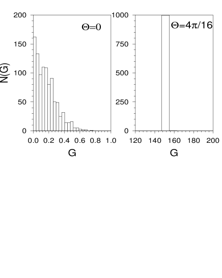
FIG. 1.: Distribution of the classification parameter G, for $\Theta$=0 and $\Theta$=4$\pi$/16.

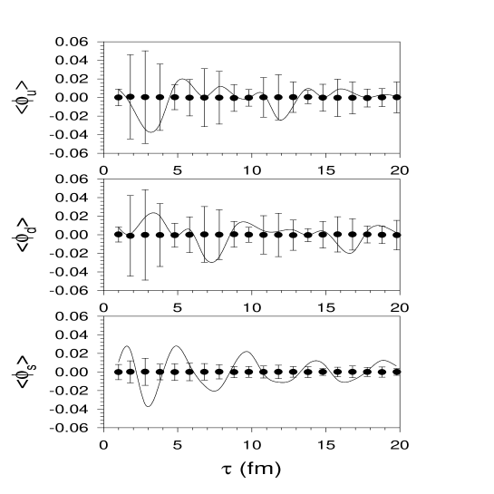
FIG. 2.: Evolution of the ensemble averaged, spatially averaged chiral phases, $\phi_{u}$, $\phi_{d}$ and $\phi_{s}$ for initial $\Theta$=0 (black circles with error bars). The solid lines show the evolution of the spatially averaged phases in the most favored event.

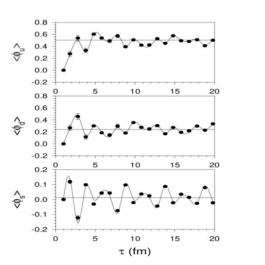
FIG. 3.: Same as fig.2 for $\Theta$=4$\pi$/16.

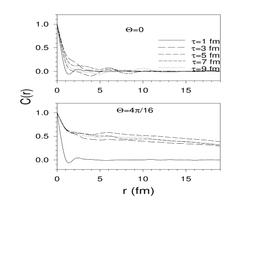
FIG. 4.: Correlation function at different times for $\Theta$=0 and $\Theta$=4 $\pi$/16, in the most favored event.

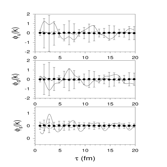
FIG. 5.: Evolution of the ensemble averaged $\phi_{i}(k)$, k=6.2 MeV (black circles with error bar), for initial $\Theta=0$. The solid, dashed, dash-dashed lines are the evolution of $\phi_{i}(k)$ in the most favored event, for k=6.2, 18.5 and 30.9 MeV respectively.

FIG. 6.: Same as Fig. 5 for $\Theta$=4 $\pi$/16

REFERENCES

- [1] e-mail address:akc@veccal.ernet.in
- [2] G. ’t Hooft, Phys. Rev. Lett. 37 (1976)8.
- [3] E. Witten, Nucl. Phys. B156 (1979),269
- [4] E. Witten, Annals Phys. 128(1980)363.
- [5] G. Veneziano, Nucl. Phys. B159 (1980)213.
- [6] D. Kharzeev, R. D. Pisarski and M. G. Tytgat, hep-ph/9804221, Phys. Rev. Lett. 81 (1998) 512.
- [7] D. Kharzeev and R. D. Pisarski, hep-ph/9906401, Phys. Rev. D61 (2000) 111901.
- [8] A. A. Anselm amd M. G. Ryskin, Phys. Lett. 266 (1991)482. Rajagopal K. and Wilczek F.,1993 B404 577. J. Bjorken, Int. J. Mod. Phys. A7 (1992)561.
- [9] D. Ahrensmeier, R. Baier, M. Dirks, Phys.Lett. B484 (2000) 58;
- [10] S. A. Voloshin, Phys.Rev. C62 (2000) 044901;
- [11] K. Buckley, T. Fugleberg, A. Zhitnitsky, hep-ph/0006057;
- [12] K. Buckley, T. Fugleberg, A. Zhitnitsky, Phys.Rev.Lett. 84 (2000) 4814.
- [13] A. K. Chaudhuri, hep-ph/0012047, Phys. Rev.(in press).
- [14] M. H. Thoma, Phys. Lett. 269B(1991)144.
- [15] I. Halperin and A. Zhitnitsky, Phys. Rev. Lett. 81 (1998)4071. T. Fugleberg, I. Halperin and A. Zhitnitsky, Phys. Rev. D59 (1999)074023.