Problems with lattice methods for electroweak preheating

Abstract

Recently Garcia Bellido et. al. have proposed that electroweak baryogenesis may occur at the end of inflation, in a scenario where the reheat temperature is too low for electroweak symmetry restoration. I show why the scenario is difficult to test reliably by classical field techniques on the lattice.

I Introduction

Inflation is a plausible and popular explanation for how the initial cosmological epoch produces a universe with such startling size, flatness, and homogeneity [1]. However, inflation makes even more puzzling the other remarkable feature of the universe–that it contains a macroscopic but relatively small net abundance of baryonic matter (approximately 5 baryons per $10^{10}$ photons [2]).

Recently Garcia-Bellido, Grigoriev, Kusenko, and Shaposhnikov have proposed a way that certain inflationary scenarios may be able to explain baryogenesis (the origin of the baryon abundance) as well [3]. During inflation, most of the energy density in the universe is in the potential energy of a scalar field, the inflaton. It has recently been understood that inflation can end, and the energy density stored in the inflaton field can be converted into a thermal bath, much more abruptly than had previously been thought possible, a process called “preheating” [4]. In the scenario of Garcia-Bellido et.al., the baryons are created during this far from equilibrium process.

Baryon number is not conserved in the standard model [5]. The violation arises from nonperturbative physics of the SU(2) weak gauge fields (W and Z bosons). When occupation numbers of infrared fields become large, nonperturbative physics can become efficient. This happens at high temperature and can also happen in other high excitation situations. In equilibrium, it occurs when there is no Higgs field condensate, which requires a temperature $T\mbox{~{}{\raisebox{1.72218pt}{$>$}} {\raisebox{-2.58334pt}{$\sim$}}~{}}100$GeV. At lower temperatures there is a Higgs field condensate and baryon number violation is exponentially slow [8]. In the Garcia-Bellido scenario, the energy density in the inflaton passes first into very infrared field modes, and baryon number is readily violated; but when the fields fully thermalize the temperature is low enough that there is a Higgs field condensate and no further baryon number violation occurs.

The Garcia-Bellido scenario involves nonlinear, nonperturbative physics, and its quantitative study is difficult to conduct analytically. For preheating in general, classical field techniques have proven useful [9, 10]. Baryon number violation in equilibrium has also been treated accurately by classical field techniques [11, 12, 13, 14, 15], and recently these techniques have been applied to the Garcia-Bellido scenario, both in a 1+1 dimensional toy model [3, 16] and in a more realistic 3+1 dimensional setting [17].

It sounds natural to expect classical field techniques to work well for the study of the Garcia-Bellido scenario. This note will argue that there are serious complications, because in the context of 3+1 dimensional Yang-Mills theory at realistic coupling, the techniques as they exist to date contain spurious physics which can lead to “fake” early thermalization and baryon number violation. At best, classical field techniques will probably have to be modified and used with care in this context; at worst they may not be useful at all.

II Classical Yang-Mills and the Lattice

A Classical field approach

First I summarize how classical field techniques are applied to preheating. The early stage of preheating can be understood analytically. When the inflaton field condensate begins to oscillate about its potential minimum, certain field modes coupled to it have their field amplitudes grow exponentially due to parametric resonance [4]. In [9, 10] it is shown that classical fields, initially populated with “quantum vacuum initial conditions,” give quantitatively the same behavior. Here “quantum vacuum initial conditions” means Gaussian random initial conditions in $k$ space, with mean squared excitation equal to the vacuum zero-point excitations of the relevant modes, ($\hbar=1$)

$$\langle Q^{2}(k,t_{\rm init})\rangle_{\rm q.\;vac}=\frac{1}{2\sqrt{k^{2}+m^{2}}}\,,\qquad\langle P^{2}(k,t_{\rm init})\rangle_{\rm q.\;vac}=\frac{\sqrt{k^{2}+m^{2}}}{2}\,,$$ (1)

with $Q$ and $P$ real canonical field and momentum variables. When parametric amplification has progressed the physics becomes nonlinear; but the occupation numbers of the relevant field modes are large by then, and the classical field approximation is valid. The classical field theory can be discretized on a lattice and evolved in real time by standard algorithms. This takes fully into account the nonlinear interactions of different field modes. Provided all of the interesting physics involves modes well to the infrared of the lattice spacing scale, the discretization should not disturb the physics of interest.

Such “quantum” initial conditions will not be preserved by classical field evolution; nothing prevents the energy associated with the “zero point” fluctuations, which have been turned into excitations of classical fields, from moving between Fourier components of the field. They will not do so, or will do so very slowly, if the coupling constant is small. But at finite coupling, even without an oscillating scalar (inflaton) condensate, this is not so. Instead, the lattice, classical field evolution will eventually approach the classical thermal distribution for the lattice system in question, which at weak coupling has

$$\langle Q^{2}(k)\rangle_{\rm thermal\;latt}\simeq\frac{T}{\tilde{k}^{2}+m^{2}}\,,\qquad\langle P^{2}(k)\rangle_{\rm thermal\;latt}=T\,,$$ (2)

for some $T\sim 1/a$. (By $\tilde{k}^{2}$ I mean the lattice dispersion relation, $a^{2}\tilde{k}^{2}=4\sum_{i}\sin^{2}(k_{i}a/2)$.) Note that the distribution is not Lorentz invariant–Lorentz invariance is broken by the lattice discretization–and has smaller field excitations than the vacuum ones at the largest $\tilde{k}^{2}$, but much larger field excitations in the infrared.

B Yang-Mills theory: Coulomb gauge correlators

       

       

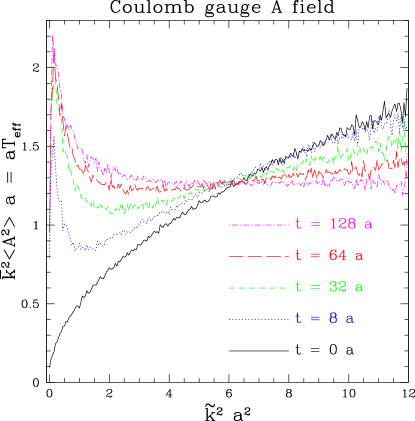
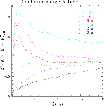
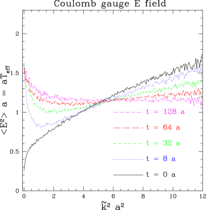
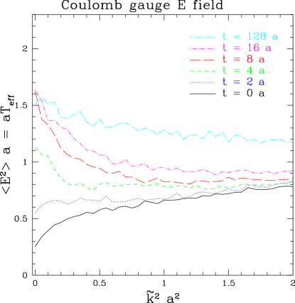
FIG. 1.: Equal time correlators in Fourier space, for classical lattice SU(2) theory at realistic coupling $g_{\rm w}=0.64$, evaluated in Coulomb gauge, at a series of times after “vacuum” initial conditions are drawn as described in the text. Top panels show $\langle\tilde{k}^{2}A^{2}(k,t)\rangle$, bottom panels show $\langle E^{2}(k,t)\rangle$; up to interaction effects, the results can be interpreted as “$k$ dependent temperatures.” The right panels show a close up of the small $\tilde{k}^{2}$ region, and earlier times. In equilibrium at zero coupling each curve would be flat; the equilibrium $E$ field curve is not flat because of Gauss’ Law, and the $A$ field curve is not flat because of interactions.

This is potentially problematic for the case at hand because the very infrared physics is the physics of interest. Eventually, the energy in the UV modes will cascade into the IR modes in a manner impossible in the actual quantum theory of interest. The question is: On what time scale does this occur? We should test whether this takes place on a time scale short enough to disturb the physics which is of interest to the simulations. The theory of interest is SU(2) Higgs theory in 3+1 dimensions, at realistic coupling. A simple way to test the viability of the classical technique is to examine the case where there is no condensate, to see how the “vacuum” fields evolve classically in isolation. If the time scale for poor behavior is shorter than the time scale for “interesting” behavior when the dynamics of interest is present, there is a problem.

We need some measurables for our study, which can indicate whether the cascade of energy into the IR has occurred; I choose to study the equal time two-point function in Coulomb gauge, as a function of $k$. Coulomb gauge is not expected to give sensible results for unequal time correlators because the gauge fixing procedure treats each time slice separately, except for a single global time dependent gauge freedom. However, for equal time correlators it should give sensible results, although it is unclear exactly how to interpret the most infrared modes. For wave numbers where perturbation theory is useful, we can interpret the values of the Coulomb gauge fixed correlation functions in terms of a $k$ dependent “effective temperature,” similar to what is done in scalar field studies of inflation. We see from Eq. (2) that the effective $k$ dependent temperature is

$$T_{\rm eff}(k,A)=\frac{1}{2}(\tilde{k}^{2}+m^{2})\langle A_{i}^{2}(k)\rangle\,,\qquad T_{\rm eff}(k,E)=\frac{1}{2}\langle E_{i}^{2}(k)\rangle\,,$$ (3)

where the factor of $1/2$ accounts for the two transverse modes summed over in the index trace; the longitudinal mode of $A$ is fixed to zero by the Coulomb gauge fixing procedure, and the longitudinal mode of $E$ is set zero, to leading order in perturbation theory, by the Gauss constraint. The above procedure also defines $T_{\rm eff}$ even where perturbation theory does not apply, but it is not clear how to interpret the result. Due to interactions, even in equilibrium $T_{\rm eff}(k)$ will not be constant for all $k$, nor will it be equal for $A$ and $E$ fields; but wherever the behavior is close to free field behavior, $T_{\rm eff}(k)$ will be approximately flat and approximately the same for $A$ and $E$ fields.

Since the cascade of energy, in the gauge sector, should be at least as fast in the full theory as in just Yang-Mills theory, and since Yang-Mills theory has fewer parameters, I study just Yang-Mills theory. Hence, $m^{2}=0$. The initial conditions are chosen as follows. All field and momentum variables are chosen as in Eq. (1), then the $E$ fields are projected to the Gauss constraint surface; the presence of longitudinal $A$ field excitations in this choice of initial conditions is irrelevant because fixing to Coulomb gauge will remove them. This is the same procedure for choosing initial conditions as was used by Rajantie et. al. [17]. Note that there is only one length scale, $a$, in the problem, and the gauge coupling is $a$ independent, so all behavior scales as $a$ is changed; the behavior of a mode of wave number $k$ depends only on $ak$.

Figure 1 shows how the field excitations evolve with time when we choose initial conditions as in Eq. (1) at gauge coupling $g_{w}=0.64$, on a $64^{3}$ lattice. The striking feature in the figure is that the infrared excitations ($k^{2}a^{2}<1/3$) are populated nearly to their thermal value very early after the evolution begins; they are largely populated by $t=8a$ and fully populated at $t=16a$. Then, over a much longer time scale, the ultraviolet modes thermalize among themselves.

C Diffusion of Chern-Simons number

FIG. 2.: Diffusion of Chern-Simons number, starting from “vacuum quantum” initial conditions, in a $32^{3}$ box at $g_{w}=0.64$. The band of error bars show the mean square value of $N_{\rm CS}$ as defined in the text; the stars indicate the mean squared values of the topological, integer part of $N_{\rm CS}$. Efficient baryon number violation begins at $t\simeq 10a$. Data at all $t$ values are from the same set of time evolutions, so the errors are highly correlated; the integer measurement was performed on a subset of the data used for the band of error bars, and have errors about $50\%$ larger.

A possible objection to this gauge theory study is that it focused on gauge fixed observables. One should always treat gauge fixed measurements with care, so I also study baryon number violation directly. The chiral anomaly relates the baryon number to the Chern-Simons number,

$$\frac{1}{3}N_{\rm B}(A_{i})=N_{\rm CS}(A_{i})\equiv\frac{g^{2}}{8\pi^{2}}\int_{A_{i}^{\prime}=0}^{A_{i}^{\prime}=A_{i}}\!\!\!d\tau\int\!d^{3}x\;\left[B_{i}^{a}(A_{\mu}^{\prime})\,D_{\tau}{A_{i}^{a}}^{\prime}\right]\,,$$ (4)

where $\tau$ parameterizes a path through the space of 3-dimensional gauge fields from the vacuum to the gauge field of interest. As defined here $N_{\rm CS}$ modulo 1 is gauge invariant; the integer part depends on the path choice. Choosing the path to coincide with the real time field evolution, the ensemble average of $N_{\rm CS}^{2}$, $\langle N_{\rm CS}^{2}\rangle$, will grow linearly in time when baryon number violation is active. Since $N_{\rm CS}^{2}$ also has a large “noise” contribution from UV excitations [12] it is more convenient to measure $N_{\rm CS}$ not of the actual configurations in a field evolution but of “cooled” copies; this is discussed in [14], and extensively in [19], which also describes the algorithm used here.

Figure 2 shows $\langle N_{\rm CS}^{2}\rangle$ as a function of time, averaged over about 1000 trajectories with independent initial conditions, on a $32^{3}$ lattice and using a cooling depth (defined in [19]) of $7.5a^{2}$. It also shows the average of the square of the integer part of $N_{\rm CS}$ (the stars, which are based on a subset of about 400 of the trajectories, and therefore have correlated and somewhat larger errors). The integer part is defined as the difference between evaluating Eq. (4) for $N_{\rm CS}(t)$ using the time history as the path, and using the cooling path from $A_{i}(t)$ to the vacuum as the path. It is a topological number which directly measures whether genuine topology change has occurred. If the vacuum state were preserved by the time evolution, we would expect $\langle N_{\rm CS}^{2}\rangle$ to fluctuate about an average close to zero, and the topological number would remain strictly zero. Instead, the figure shows that there is a brief initial period where this occurs; then, by $t=10a$, $N_{\rm CS}$ begins to diffuse at roughly the same rate it does after full thermalization. This means that, at the physical value of the coupling $g_{w}=0.64$, the IR gauge fields relevant for baryon number violation thermalize by about $t=10a$, and baryon number proceeds from there. This effect is entirely an artifact of using classical lattice evolution with “quantum zero point” initial conditions rather than treating the actual quantum theory, where baryon number, in vacuum and at this coupling, is exponentially suppressed with a large exponent. The time scale for this “artifact” baryon number violation to begin quite short; in particular it is shorter than the time scale on which Rajantie et.al. report nontrivial baryon number violating physics in the Garcia-Bellido scenario [17], by almost a factor of 3. This brings seriously into question the reliability of their results.

D Comparison to the scalar theory case

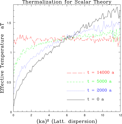
FIG. 3.: Time development of equal time $\dot{\phi}$ correlator in Fourier space for two component scalar field theory. Thermalization is slow and does not proceed first for the infrared modes, as it does in the gauge theory case.

For comparison, and because it bears on the classical field theory techniques applied in preheating [9, 10], I have also analyzed a two component scalar field theory with Lagrangian

$${\cal L}=\int d^{3}x\frac{1}{2}\left(\nabla\phi_{1}^{2}+\nabla\phi_{2}^{2}\right)+\frac{m^{2}}{2}\left(\phi_{1}^{2}+\phi_{2}^{2}\right)+\frac{\lambda}{4}\left(\phi_{1}^{2}+\phi_{2}^{2}\right)^{2}\,.$$ (5)

This theory behaves very differently from the gauge theory; indeed, even at quite large coupling the time scale for thermalization turns out to be very long. In Figure 3 I show how the power spectrum (which is now a gauge invariant quantity) evolves at the quite large coupling value of $\lambda=1$, and bare mass squared $a^{2}m^{2}=-.82\lambda$, chosen to approximately cancel a “tadpole” contribution so the initial behavior is close to that of a massless theory. The figure shows $T_{\rm eff}(k,P)$, the effective temperature derived from the momentum degrees of freedom, only; in thermal equilibrium this will be a flat line (up to statistical fluctuations) at any value of the coupling. The figure shows that, in the scalar field case, the thermalization is very slow, even at $\lambda=1$, and it proceeds across all $\tilde{k}^{2}$ values at about the same rate. Since the preheating literature generally deals with much weaker couplings, this suggests that classical lattice techniques can be reliable in the preheating context, unless the time scale of the interesting physics is extremely long.

III Discussion

We have shown that classical Yang-Mills theory, regulated on a lattice and given “quantum vacuum” initial conditions, shows very rapid heating of the infrared modes, and then more gradual thermalization between all modes. The time scale for heating of the infrared, for SU(2) at realistic coupling $g_{\rm w}=0.64$, is of order 10 lattice spacings of time (independent of the lattice spacing). This is probably faster than any purely infrared, nonequilibrium dynamics of interest will develop, which makes it difficult to study baryogenesis at preheating without the results being contaminated by artifacts of the lattice technique.

The physical reason for the rapid transfer of energy between hard and soft degrees of freedom can best be understood in the language of plasma physics. The excitations established for ultraviolet degrees of freedom, intended to simulate their quantum zero point fluctuations, propagate nearly ballistically. However, because the theory is nonabelian, they carry nonabelian “charge,” and constitute a plasma in which the IR fields evolve. The plasma degrees of freedom (UV lattice modes) move in the background of the IR modes of interest, and influence their evolution rather as a plasma modifies the evolution of infrared electromagnetic fields. It has long been appreciated that such a plasma strongly modifies the dispersion relations of the soft excitations (Debye screening, plasma oscillations, etc.), and efficiently changes the amplitude of soft excitations via Landau damping. In the nonabelian context, for quantum, equilibrium situations, this physics is contained in the “hard thermal loops” of Braaten and Pisarski [20]. An extension to the classical, lattice setting has been addressed by Arnold [21]. The damping away of large gauge field excitations is efficient below the scale $k\sim g/a$ (in a thermal plasma the scale would be $k\sim gT$). However, damping is a two way street; the time scale for a large IR field to be damped away is also the time scale for UV couplings to populate that IR field, at a “temperature” corresponding to some average over the effective temperatures of the UV degrees of freedom responsible for the damping. In the simulations of this paper, no large initial field exists; so we only see the populating of the IR modes, to an “effective temperature” of order an average over the temperatures implied by the excitation levels of the UV modes. This is approximately what we see in Figure 1; the IR modes with $k\mbox{~{}{\raisebox{1.72218pt}{$<$}} {\raisebox{-2.58334pt}{$\sim$}}~{}}gT$ are quickly excited to an effective temperature comparable to the effective temperature of the UV modes; then over a longer time scale, less infrared modes also thermalize.

Are these lattice artifact physics effects relevant for the study of the Garcia-Bellido scenario, where besides the “vacuum” excitation I have addressed, there is also large, coherent initial infrared field physics? I will argue that they are, and that they seriously complicate the analysis of the Garcia-Bellido proposal by lattice means.

The interesting physics in the Garcia-Bellido scenario is infrared, large occupation number physics. We must make the length scales associated with that physics (say, the wavelength of modes driven on resonance) much larger than the lattice spacing, or else the interesting physics will directly be contaminated by lattice effects. Therefore the time scale on which the nontrivial IR dynamics is expected to occur is quite generically long compared to the lattice spacing $a$. For instance, the interesting dynamics in the simulations of Rajantie et. al. [17] occurs at $t\sim 30a$ after the beginning of the simulation. Therefore we can expect that the excitation of the IR gauge field modes by their coupling to the UV should already have taken place before the interesting IR physics is complete.

If the actual (quantum, nonequilibrium) dynamics of interest fails to excite large IR gauge fields, then in the simulations we will nevertheless see large IR gauge fields excited, by the coupling to the UV described here. There is therefore clearly the possibility of a “false positive” indication of baryon number violation (if for instance Higgs symmetry is briefly restored, but in the actual dynamics the gauge fields would be too cold to violate baryon number). Perhaps less obviously, it is also possible that the coupling to the UV lattice modes will create “false negative” results where baryon number violation actually should occur. This could happen if the true (quantum, nonequilibrium) dynamics actually excites the IR gauge fields very efficiently, to an effective temperature higher than what the UV modes would supply. In this case, the UV modes represent an efficient absorber of the IR gauge field excitation energy, via Landau damping. In the real (vacuum, quantum) theory, energy loss to the UV should not be too efficient, and should occur mainly by a cascade. On the lattice, the UV lattice modes can directly Landau damp away large IR gauge fields on a time scale $\sim 10a$, short compared to the (expected) dynamic timescale for the nontrivial IR dynamics. Note that the UV modes also change the dispersion of the lattice modes, which means that the evolution may be wrong even if energy is not transferred to the UV. One very basic way of checking for some of these problems is to test for lattice spacing dependence in the results. This was not done in [17].

It is possible that there are ways of evading the problems discussed here. For instance, one could choose initial conditions in which only excitations with $\tilde{k}^{2}$ below some cutoff were excited. But it is not obvious that this treatment will reproduce the correct (quantum) treatment either. The physics of interest probably involves energy moving from a condensate into IR modes, and then cascading into the UV. Will this cascade be incorrectly described if the UV modes start out with no excitation? Does failing to quantize the UV modes already ensure that the description cannot be correct? The burden of proof clearly lies with the practitioner. It would be necessary but not sufficient to demonstrate that all simulation results show weak dependence on the choice of $\tilde{k}^{2}$ cutoff.

The behavior we have seen should not be expected in 1+1 dimensional, abelian studies of baryogenesis at preheating, such as those of Garcia-Bellido et. al. [3, 16]. This is a matter of dimensionality. In 3+1 dimensions, thermal self-energy corrections are UV divergent in a classical theory, with the divergence cut off in nature at $k\sim T$ by quantum mechanics. However, in 1+1 dimensions thermal self-energies are UV finite. Therefore the studies of the 1+1 dimensional abelian analog theory in [3, 16] are deceptive. The behavior I describe also appears to play little role in abelian Higgs theory, at least at the unrealistically small coupling considered in [22]. I should also emphasize that my results do not mean that previous studies of inflationary preheating are incorrect. As Figure 3 shows, the time scale for UV energy to cascade to the IR in a scalar theory, even at the very large coupling of $\lambda=1$, is very long, thousands of lattice units of time. The cascade time is expected to grow at weak coupling as $\lambda^{-2}$. The largest value of $\lambda$ used in [10] was about two orders of magnitude smaller than that in Fig. 3, so the time scale for the cascade to occur in their work would be at least $10^{7}$ lattice units, much longer than any time scale they considered. Physically this difference is related to the fact that the hard thermal loop for a gauge field contains an imaginary (Landau damping) part, while that for a scalar field does not.

REFERENCES

- [1] A. H. Guth, Phys. Rev. D 23, 347 (1981).
- [2] See for instance J. M. O’Meara, D. Tytler, D. Kirkman, N. Suzuki, J. X. Prochaska, D. Lubin and A. M. Wolfe, Astrophys. J. 552, 718 (2001) [astro-ph/0011179].
- [3] J. Garcia-Bellido, D. Y. Grigoriev, A. Kusenko and M. Shaposhnikov, Phys. Rev. D 60, 123504 (1999) [hep-ph/9902449].
- [4] J. H. Traschen and R. H. Brandenberger, Phys. Rev. D 42, 2491 (1990); L. Kofman, A. D. Linde and A. A. Starobinsky, Phys. Rev. Lett. 73, 3195 (1994) [hep-th/9405187].
- [5] G. ’t Hooft, Phys. Rev. Lett. 37, 8 (1976).
- [6] K. Osterwalder and E. Seiler, Annals Phys. 110, 440 (1978); T. Banks and E. Rabinovici, Nucl. Phys. B 160, 349 (1979); E. H. Fradkin and S. H. Shenker, Phys. Rev. D 19, 3682 (1979).
- [7] K. Kajantie, M. Laine, K. Rummukainen and M. Shaposhnikov, Phys. Rev. Lett. 77, 2887 (1996) [hep-ph/9605288].
- [8] P. Arnold and L. D. McLerran, Phys. Rev. D 36, 581 (1987).
- [9] S. Y. Khlebnikov and I. I. Tkachev, Phys. Rev. Lett. 77, 219 (1996) [hep-ph/9603378]; S. Y. Khlebnikov and I. I. Tkachev, Phys. Lett. B 390, 80 (1997) [hep-ph/9608458].
- [10] T. Prokopec and T. G. Roos, Phys. Rev. D 55, 3768 (1997) [hep-ph/9610400]; B. R. Greene, T. Prokopec and T. G. Roos, Phys. Rev. D 56, 6484 (1997) [hep-ph/9705357].
- [11] J. Ambjorn, T. Askgaard, H. Porter and M. E. Shaposhnikov, Nucl. Phys. B 353, 346 (1991).
- [12] J. Ambjorn and A. Krasnitz, Phys. Lett. B 362, 97 (1995) [hep-ph/9508202].
- [13] G. D. Moore and N. Turok, Phys. Rev. D 56, 6533 (1997) [hep-ph/9703266].
- [14] J. Ambjorn and A. Krasnitz, Nucl. Phys. B 506, 387 (1997) [hep-ph/9705380].
- [15] See for instance, G. D. Moore, C. Hu and B. Muller, Phys. Rev. D 58, 045001 (1998) [hep-ph/9710436]; D. Bodeker, Phys. Lett. B 426, 351 (1998) [hep-ph/9801430]; D. Bodeker, G. D. Moore and K. Rummukainen, Phys. Rev. D 61, 056003 (2000) [hep-ph/9907545].
- [16] J. Garcia-Bellido and D. Y. Grigoriev, JHEP 0001, 017 (2000) [hep-ph/9912515]; D. Grigoriev, hep-ph/0006115.
- [17] A. Rajantie, P. M. Saffin and E. J. Copeland, Phys. Rev. D 63, 123512 (2001) [hep-ph/0012097].
- [18] J. E. Mandula and M. Ogilvie, Phys. Lett. B 185 (1987) 127.
- [19] G. D. Moore, Phys. Rev. D 59, 014503 (1999) [hep-ph/9805264].
- [20] E. Braaten and R. Pisarski, Nucl. Phys. B337, 569 (1990); J. Frenkel and J. Taylor, Nucl. Phys. B334, 199 (1990);
- [21] P. Arnold, Phys. Rev. D 55, 7781 (1997) [hep-ph/9701393].
- [22] A. Rajantie and E. J. Copeland, Phys. Rev. Lett. 85, 916 (2000) [hep-ph/0003025].